Power laws and Self-Organized Criticality
in Theory and Nature

Abstract

Power laws and distributions with heavy tails are common features of many complex systems. Examples are the distribution of earthquake magnitudes, solar flare intensities and the sizes of neuronal avalanches. Previously, researchers surmised that a single general concept may act as an underlying generative mechanism, with the theory of self organized criticality being a weighty contender.

The power-law scaling observed in the primary statistical analysis is an important, but by far not the only feature characterizing experimental data. The scaling function, the distribution of energy fluctuations, the distribution of inter-event waiting times, and other higher order spatial and temporal correlations, have seen increased consideration over the last years. Leading to realization that basic models, like the original sandpile model, are often insufficient to adequately describe the complexity of real-world systems with power-law distribution.

Consequently, a substantial amount of effort has gone into developing new and extended models and, hitherto, three classes of models have emerged. The first line of models is based on a separation between the time scales of an external drive and a an internal dissipation, and includes the original sandpile model and its extensions, like the dissipative earthquake model. Within this approach the steady state is close to criticality in terms of an absorbing phase transition. The second line of models is based on external drives and internal dynamics competing on similar time scales and includes the coherent noise model, which has a non-critical steady state characterized by heavy-tailed distributions. The third line of models proposes a non-critical self-organizing state, being guided by an optimization principle, such as the concept of highly optimized tolerance.

We present a comparative overview regarding distinct modeling approaches together with a discussion of their potential relevance as underlying generative models for real-world phenomena. The complexity of physical and biological scaling phenomena has been found to transcend the explanatory power of individual paradigmal concepts. The interaction between theoretical development and experimental observations has been very fruitful, leading to a series of novel concepts and insights.

1 Introduction

Experimental and technological advancements, like the steady increase in computing power, makes the study of natural and man-made complex systems progressively popular and conceptually rewarding. Typically, a complex system contains a large number of various, potentially non-identical components, which often have an internal complex structure of their own. Complex systems may exhibit novel and emergent dynamics arising from local and nonlinear interactions of the constituting elements. A prominent example for an emergent property, and possibly the phenomenon observed most frequently in real-world complex systems, is the heavy-tailed scaling behavior of variables describing a structural feature or a dynamical characteristic of the system. An observable is considered to be heavy-tailed if the probability of observing extremely large values is more likely than it would be for an exponentially distributed variable [53].

Heavy-tailed scaling has been observed in a large variety of real-world phenomena, such as the distribution of earthquake magnitudes [129], solar flare intensities [41], the sizes of wildfires [121], the sizes of neuronal avalanches [89], wealth distribution [99], city population distribution [121], the distribution of computer file sizes [44, 66], and various other examples [5, 78, 121, 118, 32, 19, 2].

Notably there are many types of distributions considered to be heavy-tailed, such as the Lévy distribution, the Cauchy distribution, and the Weibull distribution. Still, investigations often focus on heavy-tailed scaling in its simplest form, the form of a pure power law (viz the Pareto distribution). In fact, it is difficult to differentiate between various functional types of heavy tails on a finite interval, especially if the data have a large variance and if the sample size is relatively small. In Fig. 1 we illustrate the behavior of three distribution functions characterized by heavy tails, the Pareto, the log–normal and the log–Cauchy probability distributions $p(x)$ (left panel), and their corresponding complementary cumulative probability distributions (CCDF) $C(x)=\int_{x}^{\infty}p(x^{\prime})\textrm{d}x^{\prime}$ (right panel). The respective functional forms are given in Table 1. In spite of having more complex scaling properties, log–normal and log–Cauchy distributions can be approximated on a finite interval by a power law, that is by a straight line on a log–log plot. Note that the difference between log–Cauchy and Pareto distribution is more evident when $C(x)$ is compared.

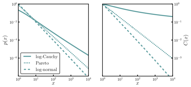
Figure 1: Comparison of different types of heavy-tailed distributions. Log–Cauchy ($\sigma=3,\mu=0$), Log–normal distribution ($\sigma=10,\mu=-100$) and Pareto distribution ($a=1.75$, see Table 1). Left: The probability distribution function $p(x)$. Right: The corresponding complementary cumulative probability distribution $C(x)=\int_{x}^{\infty}p(x^{\prime})dx^{\prime}$. The distributions $p(x)$ were normalized on the range $x\in[1,\infty)$.

Clauset et al. [32] have argued, that statistical methods traditionally used for data analysis (e.g. least-square fits) often misestimate the parameters describing heavy-tailed data sets, and consequently the actual scaling behavior. For a more reliable investigation of the scaling behavior one should employ methods going beyond visually fitting data sets with power laws, such as maximum likelihood estimates and cross-model validation techniques. Additionally, one should take into account the fact that most empirical data need to be binned [160], a procedure that reduces the available data resolution.

Large data sets, spanning several orders of magnitudes, are needed to single out the model which best fits the data and reproduces the heavy tail; even when advanced statistical techniques are applied. The collection of significantly larger data sets is however often difficult to achieve through experimental studies of large-scale complex systems, which often deal with slowly changing phenomena in noisy environments. Using rigorous statistical methods, Clauset et al. [32] re-analyzed data sets for which a least-square fit did indicate power-law scaling. They found that in some cases the empirical data actually exhibit exponential or log–normal scaling, whereas in other cases a power law, or a power law with an exponential cutoff, remains a viable description—as none of the alternative distributions could be singled out with statistical significance. Thus, in the absence of additional evidence, it is best to assume the simplest scaling of the observed phenomena, adequately described with the Pareto distribution.

Over the past decades various models have been developed in order to explain the abundance of power-law scaling found in complex systems. Some of these power-law generating models were developed for describing specific systems, and have hence only a restricted applicability. Other models, however, aim to explain universal properties of a range of complex systems. They have enjoyed significant success and contributed to the development of the paradigm that power laws emerge naturally in real-world and man-made complex systems.

name	$\displaystyle p(x)$	$\displaystyle C(x)$
Pareto	$\displaystyle x^{-\alpha}$	$\displaystyle x^{-\alpha+1}$
Log–normal	$\displaystyle\frac{1}{x}e^{-\frac{(\ln(x)-\mu)^{2}}{2\sigma^{2}}}$	$\displaystyle\frac{1}{2}\textrm{erfc}\left(\frac{\ln(x)-\mu}{2\sigma^{2}}\right)$
Log–Cauchy	$\displaystyle\frac{1}{x\left(1+\left(\frac{\ln x-\mu}{\sigma}\right)^{2}\right)}$	$\displaystyle\frac{1}{\pi}\textrm{arccot}\left(\frac{\ln(x)-\mu}{\sigma}\right)$

Table 1: Functional form of the Pareto, Log–normal and Log–Cauchy distribution $p(x)$ and the corresponding complementary cumulative distribution, $C(x)=\int_{x}^{\infty}p(x^{\prime})dx^{\prime}$.

The seminal work of Bak et al. [7] developed into an influential theory which unifies the origins of the power-law behavior observed in different complex systems—the so called theory of self-organized criticality (SOC). An important role for the success of SOC is the connection to the well-established theory of second order phase transitions in equilibrium statistical mechanics, for which the origin of scale-free behavior is well understood. The basic idea of SOC is that a complex system will spontaneously organize, under quite general conditions, into a state which is at the transition between two different regimes, that is at a critical point, without the need for external intervention or tuning. At such spontaneously maintained phase transition a model SOC system exhibits power-law scaling of event sizes, event durations and, in some cases, the $1/f$ scaling of the power spectra. These properties were also observed, to a certain extent, in natural phenomena such as earthquakes, solar flares, forest fires, and, more recently, neuronal avalanches.

In the following chapters we will discuss in more detail the pros and cons of the SOC theory and its application to real-world phenomena. In Figure 2 we show the CCDF of some of the empirical data sets analyzed in [32]. Note, that none of the shown quantities exhibit power-law-like scaling across the entire range of observations.

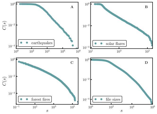
Figure 2: Log-log plots of the CCDF $C(s)$—a probability of observing an event equal to or larger than $s$—from the following empirical data sets: (A) the intensities of earthquakes occurring in California between 1910 and 1992, (B) peak gamma-ray intensity of solar flares between 1980 and 1989, (C) the sizes in acres of wildfires occurring on US federal land between 1986 and 1996 (data provided on-line by Clauset et al. [32]), (D) the sizes in Kbytes of publicly available files on the Internet [66].

SOC is observed in a range of theoretical models. However, several additional features characterize real-world complex systems and these features are mostly not captured by the standard modeling approach within the SOC framework. For example, power-law scaling in heterogeneous or noisy environments, or complex dynamics with dissipative components [77], are common features of real-world systems. As an alternative to SOC, Carlson and Doyle [23] proposed a mechanism called highly optimized tolerance (HOT) and argued that power-law distributions can manifest themselves in systems with heterogeneous structures, as a consequence of being designed to operate optimally in uncertain environments; either by human design in the case of man-made systems, or by natural selection in the case of living organisms. The HOT mechanism does not require critical dynamics for the emergence of heavy-tailed scaling.

In the following chapters we will describe in more details the main concepts of SOC and HOT, together with several other proposals for power-law generating mechanisms, and we will discuss their successes and limitations in predicting and explaining the dynamical behavior and the structure of real-world complex systems. In this context we will provide an assessment, in comparison with theory predictions, of reported statistical properties of the empirical time series of earthquake magnitudes, solar flares intensities and sizes of neuronal avalanches. In addition we will discuss the theory of branching processes and the application of critical branching to the characterization of the dynamical regime of physical systems. Another important question—that we will address and discuss within the framework of vertex routing models—is to which extent critical dynamical systems actually show power-law scaling and how the process of experimentally observing a critical system influences the scaling of the collected data.

2 Theory of Self-Organized Criticality

In their seminal work Bak et al. [7] provided one of the first principles unifying the origins of the power law behavior observed in many natural systems. The core hypotheses was that systems consisting of many interacting components will, under certain conditions, spontaneously organize into a state with properties akin to the ones observed in a equilibrium thermodynamic system near a second-order phase transition. As this complex behavior arises spontaneously without the need for external tuning this phenomena was named Self-organized Criticality (SOC).

The highly appealing feature of the SOC theory is its relation to the well established field of the phase transitions and the notion of universality. The universality hypothesis [81] groups critical phenomena, as observed for many different physical phase transitions, into a small number of universality classes. Systems belonging to the same universality class share the values of critical exponents and follow equivalent scaling functions [154]. This universal behavior near a critical point is caused by a diverging correlation length. The correlation length becomes much larger than the range of the microscopic interactions, thus the collective behavior of the system and its components becomes independent of its microscopic details. This also implies that even the simplest model captures all the aspects of critical behavior of the corresponding universality class.

Physical systems which are believed to exhibit SOC behavior are also characterized by a constant flux of matter and energy from and to the environment. Thus, they are intrinsically non-equilibrium systems. The concept of universality is still applicable to non-equilibrium phase transitions. However, an universal classification scheme is still missing for non-equilibrium phase transitions and the full spectrum of universality classes is unknown; it may be large or even infinite [103, 74]. The properties of non-equilibrium transitions depend not only on the interactions but also on the dynamics. In contrast, detailed balance – a necessary precondition for a steady state [136] – constrains the dynamics in equilibrium phase transitions.

Classification methods of non-equilibrium phase transition are diverse and phenomenologically motivated. They have to be checked for each model separately and, as analytic solutions are in most cases missing, one uses numerical simulations or renormalization group approaches to describe the behavior at the critical point. Still, as Lübeck [103] pointed out, a common mistake is the focus on critical exponents and the neglect of scaling functions, which are more informative. Determining the functional behavior of scaling functions is a precise method for the classification of a given systems into a certain universality class. The reason for this is that the variations of scaling exponents between different universality classes are often small, whereas the respective scaling functions may show significant differences. Thus, to properly determine the corresponding universality class, one should extract both scaling functions and scaling exponents.

AST	absorbing state transition
SOqC	self organized quasi criticality
BTW sandpile model	the original sandpile model
	proposed by Bak et al. [7]
Manna sandpile model	a variation of the BTW model with a stochastic
	distribution of grains, proposed by Manna [105]
OFC earthquake model	a dissipative sandpile model,
	proposed by Olami et al. [123]
Zhang sandpile model	a non-abelian variation of the BTW model
	with continuous energy, proposed by Zhang [173]

Table 2: A list of widely used acronyms and popular models for self organized criticality (SOC).

2.1 Sandpile models

The archetypical model of a SOC system is the sandpile model [7]. We will start with a general description. Sandpile models are often defined on a $d$ dimensional grid of a linear size $L$, containing $N=L^{d}$ intersecting points. A point of a grid or a lattice is called a node and to each node one relates a real or integer positive variable $h$. This variable can be seen as the local energy level, the local stress or the local height level of the sandpile (the number of grains of sand or some other particles at that location on the lattice). To mimic an external drive, that is the interaction of the system with the environment, a single node is randomly selected at each time step $t$ and some small amount of energy $\delta h$ is added to its local energy level,

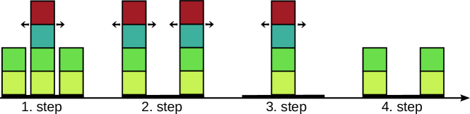
Figure 3: An illustration of particle redistribution during an avalanche for a sandpile model with three sites. Once the local height $h$ reaches the activation threshold $h_{T}=4$ the two neighboring nodes receive two particles each. Note that particles dissipate (disappear) only at the edge of the system.

$$h_{\vec{r}}(t+1)=h_{\vec{r}}(t)+\delta h\leavevmode\nobreak\ ,$$ (1)

where the index $\vec{r}=(r_{1},\ldots,r_{d})$, $r_{i}\in{1,\ldots,L}$ represents the location of a node on a $d$-dimensional lattice. If $h$ is a positive integer variable, then the increase of the local height proceeds in discrete steps, usually setting $\delta h=1$. Once the energy at some node reaches a predefined threshold value $h_{T}$, the energy configuration of the system becomes unstable, the external drive is stopped, and the local energy is redistributed in the following way:

• first, the energy level of the active node, for which $h_{\vec{r}}\geq h_{T}$, is reduced by an amount $\Delta h$, viz.

  $$h_{\vec{r}}\rightarrow h_{\vec{r}}-\Delta h\leavevmode\nobreak\ .$$ (2)

• second, the nearest neighbors of the active node, receive a fraction $\alpha$ of the lost energy $\Delta h$. Denoting with $\vec{e}_{n}$ the relative location of nearest neighbors with respect to location of active node $\vec{r}$, we can write

  $$h_{\vec{r}+\vec{e}_{n}}\rightarrow h_{\vec{r}+\vec{e}_{n}}+\beta\Delta h\leavevmode\nobreak\ .$$ (3)

  For example, in the case of two dimensional ($d=2$) lattice we have $\vec{e}_{n}=(\pm 1,0)$, $(0,\pm 1)$.

• the update is repeated as long as at least one active node remains, that is, until the energy configuration becomes stable.

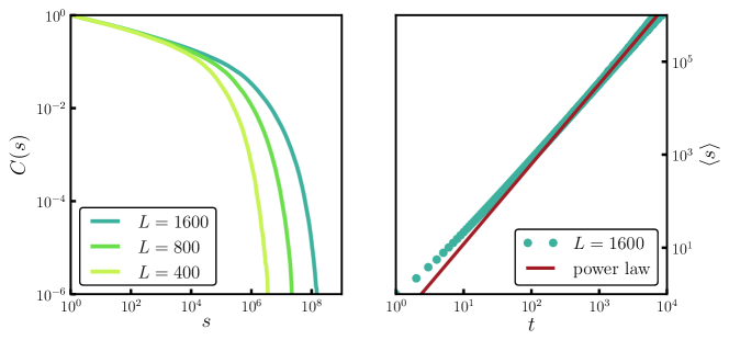
Figure 4: Left: The complementary cumulative distribution $C(s|L)=\sum_{k=s}^{s_{max}}P(k|L)$ of avalanche sizes $s$ for the BTW sandpile model on a regular lattice of linear size $L$. Right: Average size $\langle s\rangle$ of avalanches, as a function of duration $t$, compared with the power-law dependence expected from the finite size scaling Ansatz $s\sim t^{\gamma_{ST}}$ (see Eq. 6) with $\gamma_{ST}=1.46$.

In Fig. 3 we illustrated the process of particle transport among nearest neighbors, also called an avalanche. Setting

$$\beta=\frac{1}{2d}$$

assures local conservation of energy during an avalanche; a necessary condition for a true SOC behavior of the sandpile models, as we will discuss later. However, the energy is conserved only locally; it is important to allow the energy to dissipate at the lattice boundaries (grains falling off the table), which is achieved by keeping the boundary nodes empty. If the amount of transferred energy $\Delta h$ – which is transfered upon site activation – equals the threshold value $h_{T}$, one calls the model an Abelian SOC model, because in this case the order of the energy redistribution does not influence the stable state configuration reached in the end of the toppling process. The Abelian realization of the discrete height SOC model is better known as Bak-Tang-Wiesenfeld (BTW) sandpile model [7]. In addition, setting $\Delta h=\epsilon h$, where $\epsilon\in(0,1]$ leads to a non-Abelian SOC model which was – in its continuous energy form – first analyzed by Zhang [173], thus named Zhang sandpile model (see Table 2).

Beside the BTW and the Zhang sandpile models, other variations of toppling rules exist. One possibility is a stochastic sandpile model proposed by Manna [105], which was intensively studied as it is solvable analytically. Toppling rules can be divided into Abelian vs. non-Abelian, deterministic vs. stochastic and directed vs. undirected [114]. Modifications of the toppling rules employed often results in a change of the universality class to which the model belongs [13, 57].

Hitherto we described the critical height model, where the start of a toppling process solely depends on the height $h_{\vec{r}}$. Alternatively, in the critical slope model the avalanche initiation depends on the first derivative of the height function $h_{\vec{r}}$, or in the critical Laplacian model on the second derivative of the height function. These alternative stability criteria lead either to a different universality class, or to a complete absence of SOC behavior [104].

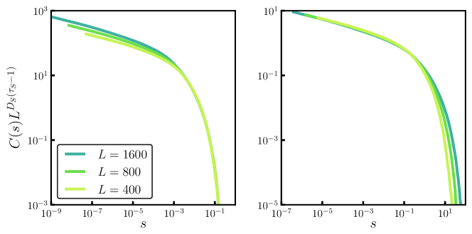
Figure 5: Finite size scaling for the two dimensional BTW sandpile model, for the data shown in Fig. 4. Shown is the rescaled complementary cumulative avalanche sized distribution CCDF, using the finite-size scaling Ansatz (4), appropriately integrated. The scaling parameters are $\tau_{S}=1.31$ and $D_{S}=2.8$ (left) and $\tau_{S}=1.15$ and $D_{S}=2$ (right). Note that the first set of scaling exponents describes large avalanches well, with the second set of exponents being appropriate for small avalanches.

2.2 Finite size scaling

The scaling behavior of avalanches can be extracted from the statistical properties of several quantities: e.g. the size $s$ of the avalanche (the total number of activations during an avalanche), the area $a$ of an avalanche (the number of distinct activated nodes), the avalanche duration $t$ (the number of parallel updates until a stable configuration is reached) and the linear size of the avalanche $r$ (usually estimated as the radius of gyration). In Fig. 4 we show distribution of avalanche sizes obtained from the simulation of the BTW sandpile on a regular two dimensional lattice. In this review we discuss the scaling of observables – like the results for the sandpile model shown in Fig. 4 – which result from uniform dynamics devoid of a hierarchical organization. Scaling exponents may become complex in the presence of underlying hierarchies [150] or specific interplay of dissipative and driving forces [96]. Hence, in such cases one needs to adopt the analysis of the scaling behavior corresponding to the discrete scale invariance [75, 177], characterized by complex scaling exponents.

The theory of equilibrium critical phenomena implies that the scaling behavior of this quantities – whenever the system is near a second-order phase transition – follows the finite-size scaling (FSS) ansatz. In other words, one expects to find a scaling function for each observable uniquely defining their respective scaling behavior, independently of the system size. Under FSS assumption probability distributions should have the following functional form [22]

$$P_{X}(x|L)=x^{-\tau_{X}}F_{X}(x/x_{c}),\qquad\quad x_{c}=L^{D_{X}}\leavevmode\nobreak\ .$$ (4)

Here $\tau_{X}$ and $D_{X}$ are the critical exponents for $x\in\{s,a,t,r\}$ and $L$ the linear system size. The scaling function $F_{X}$ describes the finite size correction to the power law. Event sizes $x$ substantially smaller than the system size follow a power law, $F_{X}\to const.$ for $x<<L^{D}$, with the fractional dimension $D_{X}$ cutting off large fluctuations, $F\rightarrow 0$ for $x\rightarrow x_{c}=L^{D_{X}}$.

When the quantities (the size, the area, etc.) all follow FSS, then they will also scale as a power of each other in the limit $L\rightarrow\infty$, that is the conditional probability $P_{X^{\prime}X}(x^{\prime}|x)$ of measuring $x^{\prime}$ given $x$ is diagonal,

$$P_{X^{\prime}X}(x^{\prime}|x)\propto\delta(x^{\prime}-{x}^{\gamma_{X^{\prime}X}})\leavevmode\nobreak\ ,$$ (5)

which arises from the requirement that $P_{X^{\prime}}(x^{\prime})=\int P_{X^{\prime}X}(x^{\prime},x)\textrm{d}x$ is satisfied for any $x,x^{\prime}\in\{s,a,t,r\}$. From the same condition one obtains the scaling laws

$$\gamma_{X^{\prime}X}=\frac{\tau_{X}-1}{\tau_{X^{\prime}}-1}\leavevmode\nobreak\ .$$ (6)

Early studies of SOC behavior have demonstrated that certain models deviate from the expected FSS Ansatz. Reason for this deviation can be found in several premises behind the FSS Ansatz: (1) boundaries should not have a special role in the behavior of the system; (2) a small finite system should behave the same as a small part of a large system. However, these conditions do not hold for most sandpile models. First, energy is dissipated at the boundaries, and their shape influences the scaling behavior. Second, the average number of activations per site increases, during large avalanches, with the size of the system [46], since energy dissipation is a boundary effect.

As an illustrative example we present in Fig. 5 the rescaled CCDF of the avalanche size $s$ for the BTW sandpile model under the FSS assumption, that is rescaling $s\rightarrow s/L^{D_{S}}$ and $C_{S}(s)\rightarrow C_{S}(s)L^{D_{S}(\tau_{S}-1)}$, with linear dimensions $L$. Depending on the value selected for the critical exponents, $\tau_{S}$ and $D_{S}$, one finds nice collapse of the data for either large or small avalanches, though not for the entire range of avalanche sizes. This behavior is consistent with the deviation from a pure power-law scaling for the time-dependent average avalanche size, as shown in Fig. 4, which may be approximated asymptotically by a power law for either short or long avalanche durations, but not for the entire range. Still, one can argue that scaling, as described by Eq. (4), is expected to hold anyhow only asymptotically in the thermodynamic limit, that is, for large avalanche sizes or durations. Hence, it is of interest to examine whether these results indicate to the presence of several distinct scaling regimes.

Figure 6: Avalanche scaling properties of the two dimensional BTW sandpile model. (left) Multifractal spectrum $f_{s}(\alpha)$ of the avalanche size distribution $P_{s}$ for varying liner sizes $L$; (right) Scaling function $\sigma_{s}(q)$ of the $q$th moment of $P_{s}$, $\langle s^{q}\rangle\sim L^{\sigma(q)}$ obtained as linear fit of $\ln\langle s^{q}\rangle(L)$. Dashed line represents the fit of the region where $\sigma_{S}$ has linear dependence. The slope of the linear fit is then used to estimate $D_{S}=2.8$ and $\tau_{S}=1.31$.

2.2.1 Multiscaling Ansatz

It is well known, for a thermodynamic phase transition, that distinct scaling regime may exists. Somewhat further away from the critical point one normally observes scaling with meanfield exponents, and close to the transition (where the degree of closeness is given by the Ginzburg criterion) the scaling exponents are determined by the underlying universality class. A possible approach in discriminating distinct scaling regimes is to perform a rescaling transformation of the observable of interest, an venue taken by the multifractal scaling Ansatz [82, 39, 156]. Rescaling the CCFF

$$f_{X}(\alpha)=\frac{\log\left(C_{X}(\alpha|L)\right)}{\log(L)},\qquad\quad C_{X}(\alpha|L)=\int^{\infty}_{L^{\alpha}}P_{X}(x|L)dx\leavevmode\nobreak\ ,$$ (7)

one obtains with $f_{X}(\alpha)$ the so-called multifractal spectrum [127]. One can furthermore define via

$$\langle x^{q}\rangle_{L}=\int P_{X}(x|L)x^{q}dx\sim L^{\sigma_{X}(q)}\leavevmode\nobreak\ ,$$ (8)

the scaling exponents $\sigma_{X}(q)$ to the $q$th moment of the distribution $P_{X}(x|L)$, which are related to the multifractal spectrum $f_{X}(\alpha)$ through a Legendre transform,

$$\sigma_{X}(q)=\textrm{sup}_{\alpha}\big{[}f_{X}(\alpha)+q\alpha\big{]}\leavevmode\nobreak\ .$$ (9)

If FSS is a valid assumption, viz when $P_{X}(x|L)$ follows a simple power law with a sharp cutoff given by $L^{D_{X}}$, then the following form for $f_{X}(\alpha)$ is expected:

$$f_{X}(\alpha)=\begin{cases}\alpha(1-\tau_{X})&\mbox{for\ \ \ }0<\alpha\leq D_{x}\\ -\infty&\mbox{for\ \ \ }\alpha_{x}>D_{x}\end{cases}\leavevmode\nobreak\ .$$ (10)

The jump to $-\infty$ is replaced by a continuous downturn whenever the upper cutoff is not sharp, viz if events of arbitrary large size $x$ are allowed but exponentially unlikely. The Legendre transform $\sigma_{X}(q)$ is given, for FSS, by

$$\sigma_{X}(q)=\begin{cases}D_{X}(q-\tau_{X}+1)&\mbox{for\ \ \ }q>\tau_{X}-1\\ \sigma_{X}(q)=0&\mbox{for\ \ \ }q<\tau_{X}-1\end{cases}\leavevmode\nobreak\ .$$ (11)

The fractal spectrum $f_{X}(\alpha)$ will be piecewise linear for distributions having well defined and well separated scale regimes. On says that a fractal spectrum shows “multifractal scaling” when linear regimes are not discernible.

In Fig. 6 we show the multifractal spectrum $f_{S}(\alpha)$ for different system sizes $L$, and the corresponding moment scaling function $\sigma_{s}(q)$, which was obtained as the slope of the linear fit of $\ln\langle s^{q}\rangle(L)$ for a fixed moment $q$. The continuous downturn for large $\alpha$ seen for $f_{S}(\alpha)$ results from the absence of a hard cutoff, the number of activated sites during an avalanche may be arbitrary large (in contrast to the area, which is bounded by $L^{d}$). One notes that data collapse is achieved and that $f_{s}(\alpha)$ and $\sigma_{s}(q)$ are not piece-wise linear, implying multiscaling behavior of the BTW sandpile model.

So far we have discussed methods typically used to characterize a scaling behavior of various SOC models, which provide a way to estimate both scaling exponents and scaling functions. In the next subsection we will discuss the underlying mechanism leading to the emergence of the critical behavior observed in various sandpile models. For this purpose we introduce a general concept well known in the theory of non-equilibrium phase transitions, the so called “absorbing phase transitions”.

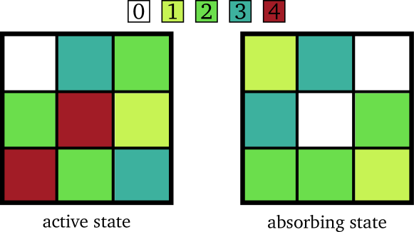
Figure 7: Random configurations of particles on $3\times 3$ periodic lattice for a fixed energy sandpile model, where the activation threshold $h_{T}=4$. Left: An active state with a large number of particles per site, $\rho>\rho_{c}$. Right: An absorbing state with a low number of particles per site, $\rho<\rho_{c}$, which is inactive.

2.3 Absorbing phase transitions and separation of time scales

Absorbing phase transitions exist in various forms in physical, chemical and biological systems that are operating far from equilibrium. They are considered without a counterpart in equilibrium systems and are studied intensively. For an absorbing phase transition to occur it is necessary that a dynamical system has at least one configuration in which the system is trapped forever, the so-called absorbing state. The opposite state is the active phase in which the time evolution of the configuration would never come to a stop, that is, the consecutive changes are autonomously ongoing.

A possible modeling venue for a dynamical system with an absorbing phase transition is given by the proliferation and the annihilation of particles, where particles are seen as abstract representation of some quantity of interest. A simple example for this picture would be a contact process on a $d$-dimensional lattice [109], which is defined in the following way: A lattice node can be either empty or occupied by a single particle; a particle may disappear with probability $1-p$ or create an offspring with probability $p$, at a randomly chosen nearest neighbor node. This contact process has a single absorbing state (with zero particles present) and one can show, in the mean field approximation, that this absorbing state becomes unstable for $p>p_{c}=1/2$. For a broader discussion and a general overview of absorbing phase transitions we refer the reader to the recent review articles [74, 103, 109, 136] and books [72, 71]. Here we will focus on the connection between the absorbing phase transitions and SOC.

To understand the nature of SOC behavior arising in sandpile models we consider a fixed energy sandpile model. This model is obtained from the standard sandpile model by removing the external drive (the random addition of particles) and the dissipation (the removal of the particles at the boundary). Still, if the number of particles on a single lattice node exceeds some threshold value $h_{T}$ the particles at that node are redistributed to neighboring nodes as given by Eq. (3). This redistribution process continues as long as there are active nodes, at some position $\vec{r}$, with $h_{\vec{r}}\geq h_{T}$. If the initial particle density $\rho$ is smaller than some critical value $\rho_{c}$ any initial configuration of particles will, in long-time limit, relax into a stable configuration, corresponding to an absorbing state. In a stable configuration there are no active nodes and each node can be in $h_{T}$ possible state (from $0$ to $h_{T}-1$). Hence, in the thermodynamic limit exist infinitely many absorbing states. For $\rho>\rho_{c}$ there is always at least one active site and the redistribution process continues forever. An illustration of absorbing and active states is shown in Fig. 7.

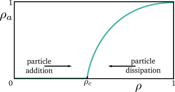
Figure 8: The average density of active particles $\rho_{a}$, the order parameter for an absorbing phase transition, as a function of particle density $\rho$. The balance between the (very slow) addition of particles and the (relatively fast) dissipation during the active phase can maintain $\rho$ at the critical value $\rho_{c}$. This separation of time scales is a defining property of processes self-organizing towards criticality.

Using the average density of active states $\rho_{a}$ as an order parameter, one usually finds that the absorbing to active phase transition is of second order, with $\rho_{a}$ changing continuously as $\rho$ goes through the $\rho_{c}$, as illustrated in Fig. 8. Thus, having a mechanism which slowly increases the amount of particles when $\rho<\rho_{c}$ (external drive) and which is stopped once the active state is reached, where fast dissipative effects take over (dissipation at the boundaries), will lead to the kind of self-organized critical phenomena as they are observed in sandpile models (Fig. 8). Hence, we can relate criticality in sandpile models to the separation of timescales between external driving process and intrinsic dissipation process in systems with absorbing phase transitions. Thus, any non-equilibrium system, exhibiting an transition from an absorbing to an active phase, can be driven to a critical point by including a driving and a dissipating mechanisms with infinite separation of time scales [42]. The separated time scales ensure the balancing of the system at the point of transition.

2.4 SOC models on different network topologies

Unlike regular structures or lattices, typically used in sandpile models, real-world complex systems mostly have non-regular structures, characterized often by a small world topology and scale-free connectivity. Thus, it is important to understand the influence of different network topologies on the scaling behavior of sandpile and other SOC models.

The studies of the sandpile dynamics on Erdős–Rényi random graphs [50], have shown that the scaling exponents correspond to the ones obtained for high-dimensional lattices [31, 15], thus belonging to the same universality class in the thermodynamic limit. Similar conclusions have been reached for the BTW sandpile on the Watts-Strogats type small-world networks [161]. This kind of networks are constructed from an usual $d$-dimensional lattice by randomly rewiring a certain fraction of links $p$. Importantly, the rewiring is performed in a way such that the number of nearest neighbors is unchanged. This introduces long range interaction for $p>0$, yielding small-world structures for small $p$ and random structures for large $p$. On these networks it is simple to implement the classical BTW model without any modification for the toppling dynamics. De Arcangelis and Herrmann [37], Pan et al. [126] concluded that the avalanche behavior, in the thermodynamic limit $L\rightarrow\infty$, corresponds to the mean field behavior for any $p>0$. Thus, the introduction of shortcuts to regular lattice structures is effectively increasing the dimensionality of the lattice, with the scaling behavior corresponding to the one observed for high dimensional lattices [92].

2.4.1 Scale-free networks

Investigations of the BTW sandpile model on uncorrelated scale-free networks [8] have shown an interesting scaling behavior dependent on the network parameters [58, 59, 95, 60]. Scale-free graphs are graphs with a power-law distributed degree, that is $p_{d}(k)\sim k^{-\gamma}$, where the degree $k$ of a node is the number of its nearest neighbors. As each node has a variable number of neighbors, the activation threshold of each node is set proportional to the local vertex degree and defined as $h_{T}^{(i)}=k_{i}^{1-\eta}$, where $k_{i}$ is the out-degree of the $i$th node, and $0\leq\eta\leq 1$ such that $h_{T}^{(i)}\leq k_{i}$. Grains of sand are again added to randomly chosen nodes, until the activation threshold $h_{T}^{(i)}$ of the selected node is surpassed. Once a node gets activated the external drive is stopped, and the toppling of grains proceeds until a stable state is reached. Dissipation is introduced either by removing small fraction $f$ of grains during the avalanche, or by mapping the network to a lattice and removing some small amount of grains at the boundary, which sets the maximal size of the avalanche. Active sites transfer a single grain to each of the $n=\lceil h_{T}^{(i)}\rceil$ randomly chosen nearest neighbors, where $\lceil h_{T}^{(i)}\rceil$ denotes the smallest integer greater or equal to $h_{T}^{(i)}$. The height of the $i$th active node $h_{i}$ is then decreased by $\lceil h_{T}^{(i)}\rceil$. Note that for $\eta>0$ the grains are stochastically redistributed to nearest neighbors as the number of available grains $n$ is smaller then the out-degree $k_{i}$.

In addition to numerical simulation, the scaling exponents for the avalanche size $\tau_{s}$ and the avalanche duration $\tau_{t}$ have been obtained analytically by taking into account the tree like structure of the uncorrelated network and by mapping an avalanche to a branching processes [94], a procedure we will discuss in Sect. 4. Using the formalism of branching processes one finds that the scaling exponents of the avalanche distributions depend on the network scaling exponent $\gamma$ and threshold proportionality exponent $\eta$ in the following manner:

$$\begin{array}[]{llcr}\tau_{s}=3/2,&\quad\tau_{t}=2&\quad\textrm{when}&\gamma>3-\eta\\ \tau_{s}=\frac{\gamma-2\eta}{\gamma-1-\eta},&\quad\tau_{t}=\frac{\gamma-1-\eta}{\gamma-2}&\quad\textrm{when}&2<\gamma<3-\eta\end{array}$$ (12)

Hence, there are two separate scaling regimes dependent on the value of the parameter $\gamma$, which defines the network connectivity. At the transition of this two regimes—that is, for $\gamma=3-\eta$—the avalanche scaling has a logarithmic correction

$$p_{s}(s)\sim s^{-3/2}(\ln s)^{-1/2},\qquad p_{t}(t)\sim t^{-2}(\ln t)^{-1}\leavevmode\nobreak\ .$$ (13)

These logarithmic corrections correspond to the scaling properties of critical systems at the upper critical dimension, above which the mean-field approximation yields the correct scaling exponents.

The analytic results (12) for uncorrelated graphs are well reproduced by numerical simulations [60]. However, real-world networks having scale-free degree distributions, contain additional topological structures, such as degree-degree correlations. Simulating the sandpile dynamics at the autonomous system level for the Internet, and for the co-authorship network in the neurosciences, one observes deviations to the random branching predictions [60]. The higher order structures of scale-free networks do therefore influence the values of the scaling exponents. In addition, separate studies of BTW sandpile models on Barabási-Albert scale-free networks have demonstrated that scaling also depends on the average ratio of the incoming and the outgoing links [85], further demonstrating the dependence of scaling behavior on the details of the topological structure of the underlying complex network.

Topological changes in the structure of the network generally do not disrupt the power-law scaling of the BTW model, it is however still worrisome that the scaling exponents generically depend on the network fine structure. Such dependencies suggests that the number of the universality classes is at least very large, and may possibly even be infinite. With so many close-by universality classes, a large database and very good statistics is hence necessary, for a reliable classification of real-world complex system through experimental observation.

In the following subsection we will consider SOC models supplemented by dissipative terms—which are essential for many real-world applications—thus contrasting the SOC models with conserved toppling dynamics which we did discuss hitherto.

2.5 SOC models with dissipation

Conventional SOC models such as BTW, Zhang or Manna sandpile models (see Table 2), require—to show critical scaling behavior—that the energy (the number of sand grains) is locally conserved. The introduction of local dissipation during an avalanche (e.g. by randomly removing one or more grains during the toppling) leads to a subcritical avalanche behavior and to a characteristic event size which is independent of the system size. To recover self-organized critical behavior—or at least quasi-critical behavior, as we will discuss later—a modification is required for the external driving. Besides the stochastic addition of particles or energy, a loading mechanism has to be introduced. This mechanism increases the total energy within the system, bringing it closer to the critical point, but without starting an avalanche [16]. From now on we will only consider models where the lattice nodes are represented by a continuous variable representing local energy levels, as defining dissipation under such setup is quite straightforward.

In recent years, SOC models without energy conservation have raised some controversy regarding the statistical properties of the generated avalanche dynamics, and with regard to their relation to the critical behavior observed in conserved SOC models, such as the BTW model. A solvable version of a non-conserving model of SOC was introduced by Pruessner and Jensen [135]. The dissipation is controlled by a parameter $\beta$ (compare Eq. 3) which determines the fraction of energy transmitted, by an activated node, to each neighbor. The toppling dynamics is conserving for $\beta=1/k$, where $k$ denotes the number of nearest neighbors, and dissipative for $0<\beta<1/k$. For the external driving one classifies the sites into three categories. A site with energy $z_{i}$ is said to be stable for $z_{i}<h_{T}(1-\beta)$, susceptible for $h_{T}(1-\beta)\leq z_{i}<h_{T}$ and active for and $1\leq z_{i}$. The actual external driving is then divided into a loading and a triggering part.

• The loading part of the external drive consists of randomly selecting $n$ nodes. If the selected sites are stable, having an energy level below $h_{T}(1-\beta)$, their respective energies are set to $h_{T}(1-\beta)$, they become susceptible.

• For the triggering part of the external driving a single node is selected randomly. Nothing happens if the site is stable. If the site is susceptible, its energy level is set to $h_{T}$ and the toppling dynamics starts.

Interestingly, depending on the loading intensity, that is on the value of the loading parameter $n$, the avalanche dynamics will be in a subcritical, critical or supercritical regime, for a given system size $N=L^{d}$. The critical loading parameter $n_{c}$ scales as a power of the system size $N$ and diverges in the thermodynamic limit. This need for fine tuning of the load, which can be generalized to other non-conservative SOC models, implies that dissipative systems exhibit just apparent self-organization. Furthermore even with tuned loading parameter $n=n_{c}$, the dynamics will only hover close to the critical state, without ever reaching it exactly. This behavior was denoted self-organized quasi-criticality (SOqC) by Bonachela and Muñoz [16].

2.5.1 The OFC earthquake model

Figure 9: An illustration of local dissipation during an avalanche, introduced in the OFC model. Besides the dissipation at the boundary, some fraction of energy (denoted by blue rectangles) is lost locally at each active site. The remaining energy is distributed equally between the neighboring nodes or dissipated at the open boundary.

Perhaps one of the most studied dissipative SOC models is the Olami-Feder-Christensen (OFC) model [123]. The OFC model is an earthquake model, as it was originally derived as a simplified version of the Burridge-Knopoff model [20], which was designed to mirror essential features of earthquakes and tectonic plates dynamics. In this model the local height parameter $h_{\vec{r}}$ is continuous and corresponds to local forces. The external driving, thought to be induced by slipping rigid tectonic plates, is global in the OFC model, whereas it would be local in most other sandpile models. The global driving force is infinitesimally slow and acts at the same time on all sites. Thus, the driving process can be simplified as following:

• One determines the location $\vec{r}^{*}$ with the largest stress, with $h_{\vec{r}^{*}}>h_{\vec{r}}$, for every position $r\neq\vec{r}^{*}$.

• All forces are then increased by $h_{\vec{r}}(t+1)=h_{\vec{r}}(t)+\delta h$, where $\delta h=h_{T}-h_{\vec{r}^{*}}$.

• The toppling dynamics then starts at $\vec{r}^{*}$, following Eq. (3), with a dissipation parameter $\beta$ and $\Delta h=h_{\vec{r}}$, that is after activation $h_{\vec{r}}(t+1)\rightarrow 0$.

The model becomes, as usual, conservative for $\beta={1}/{2d}$. In addition to the local dissipation there is still dissipation at the boundaries (see Fig. 9), when assuming fixed zero boundary forces $h_{\vec{r}}$. In fact dissipative boundaries are essential for SOqC behavior to emerge.

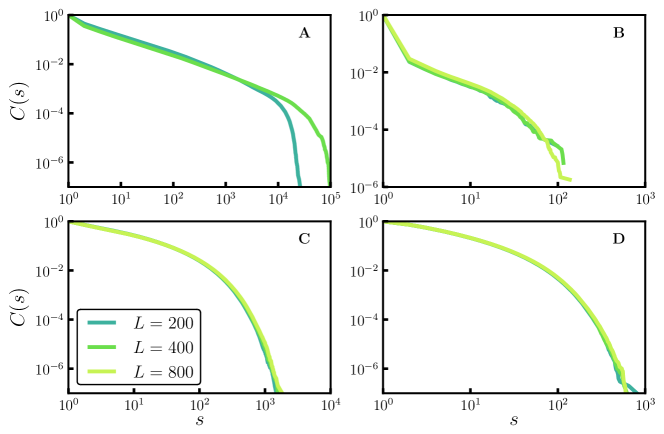
Figure 10: Complementary cumulative avalanche size distribution for dissipative OFC model on different network topologies, all having $N=L^{2}$ nodes. (A) Regular lattice with open boundaries, (B) regular lattice with periodic boundary conditions, (C) small-world network, (D) scale-free network.

Although initial studies of OFC models showed indications of critical behavior [123, 77, 78, 100], later numerical studies on much larger system sizes found little evidence for the critical scaling of avalanche sizes. For dissipation rates $\beta>0.18$ the scaling is very close to a power law and the behavior may be considered as almost critical that is quasi-critical [111, 18, 112]. The difficulty with simulating the OFC model is that system goes through a transient period, which grows rapidly with system size, before it reaches the self-organized stationary state, thus increasing significantly the computational power and time needed to simulate large lattices [166]. Furthermore, in the same work, Wissel and Drossel [166] showed that the size distribution of the avalanche is not of a power law form but rather of a log-Poisson distribution. Nevertheless, it is still considered that dissipative systems with loading mechanism are much closer to criticality than it would be the case in the absence of such mechanism [16]. Still, although the OFC model is not strictly critical, it is somewhat more successful then other similar models in fitting the Omori scaling of aftershocks [73, 166].

The OFC model, which has seen several successful applications [70, 73, 27], does neglect heterogeneities as they occur in the structure of the real-world complex systems. Within the OFC model one assumes that the site activation threshold is uniform across all nodes, that the avalanches are undirected, that the elements have symmetric interactions and that the network has a regular structure and regular dissipative boundaries. Adding local variations, expected to exist in natural systems, in any of the mentioned properties of the model, leads to the disappearance of any similarity to critical scaling behavior. For example, introducing local variations in the threshold values [77], or in the local degree of dissipation [117], results in subcritical scaling behavior, although SOqC is preserved for very small variations. The change in the network structure to more irregular topology has a similar effect, although exceptions exist. For the case of quenched random networks, only finite avalanches are observed for any non-zero dissipation level, while power-law scaling is retained for annealed networks [29, 101]. The disappearance of power-law scaling has also been observed for the OFC model on scale-free networks [26] and regular lattice with periodic boundary conditions [61] (see Fig. 10). Interestingly, OFC model on small-world topology, with a small rewiring probability and undirected connections, shows properties similar to the ones obtained on regular lattices [26]. Examples for the scaling of avalanche sizes in the presence of various site dependent irregularities for the OFC model are shown in Fig. 11.

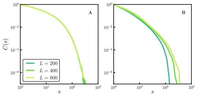
Figure 11: Cumulative avalanche size distribution for dissipative OFC model on a regular lattice in the case of (A) non-uniform threshold, (B) asymmetric and random interactions.

Non-conserving SOC models are able to reproduce certain aspects of scaling exhibited by real-world phenomena. The incorporation of structural variations, which are common features of natural and man made systems, results however in qualitative changes for the observed scaling. This circumstance is quite worrying, as pointed by Jensen [78]. If a model is applicable to real physical systems, it should also exhibit some robustness to disorder. In section 5 we will discuss in more details empirically observed properties of earthquakes and solar flares, which will also reveal additional differences between real-world phenomena and both conserved and non-conserved SOC models. The implications of SOC theory on the observed power-law behavior of neuronal avalanches, and possible extensions of SOC theory or alternative explanation of their origin, will also be discussed.

3 Alternative models for generating heavy-tailed distributions

The quest for explaining and understanding the abundance of power-law scaling in complex systems has produced, in the past several decades, a range of of models and mechanisms for the generation of power laws and related heavy-tailed distributions.

Some among these models provide relatively simple generating mechanisms [121], e.g. many properties of random walks are characterized by power laws, while others are based on more intricate principles, such as the previously described SOC mechanism. We will now shortly describe three classes of basic generating mechanism, and then discuss in more detail a recently proposed heavy-tail generating mechanism, the so called principle of highly optimized tolerance. The emphasis of our discussion will be on general underlying generating principles, and not on the details of the various models. For additional information with respect to several alternative mechanisms, not mentioned here, we refer the reader to several sources [115, 121, 151, 145].

3.1 Variable selection and power laws

One can generate power laws when selecting the quantity of interest appropriately [148, 121]. This procedure is, however, in many cases not an artifact but the most natural choice. Consider an exponentially distributed variable $y$, being logarithmically dependent on a quantity of interest $x$,

$$p(y)\sim\mathrm{e}^{ay},\quad\qquad y=b\log(x),\quad\qquad\frac{dy}{dx}=\frac{b}{x}\leavevmode\nobreak\ .$$ (14)

The distribution $p(x)$

$$p(x)=p(y)\frac{dy}{dx}\sim\frac{b}{x}\mathrm{e}^{ab\log(x)}\sim x^{ab-1}$$ (15)

then has a power-law tail. Exponential distributions are ubiquitous, any quantity having a characteristic length scale, a characteristic time scale, etc. is exponentially distributed. A logarithmic dependence $y\sim\log(x)$ does also appear frequently; e.g. the information content, the Shannon information, has this functional form [64]. Power laws may hence quite naturally arise in systems, like the human language, governed by information theoretical principles [121].

For another example consider two variables being the inverse of each other,

$$x\sim\frac{1}{y},\qquad\quad p(x)\sim\frac{p(y)}{x^{2}}\leavevmode\nobreak\ .$$ (16)

The distribution $p(x)$ has hence a power-law tail for large $x$, whenever the limit $\lim_{y\to 0}p(y)$ is well behaved. E.g. for finite $p(y=0)$ the tail is $p(x)\sim 1/x^{2}$. Whether or not a relation akin to (16) is physically or biologically correct depends on the problem at hand. It is important, when examining real-world data, to keep in mind that straightforward explanations for power-law dependencies—like the ones discuss above—may be viable, before jumping to elaborated schemes and fancy explanations.

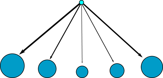
Figure 12: An illustration of the Yule process. A probability that a newly created unit (top node) joins one of the existing communities (lower nodes) is proportional to the size of that community, indicated by the respective sizes of the nodes.

3.2 Growth processes directed by importance measures

One of the most applied principle, comparable to the success of SOC theory, is the Yule Process [168] or the “rich-gets-richer” mechanism, which was originally introduced to explain the power-law distribution of sizes of biological taxa. Later other researchers adapted and generalized the Yule process for the power-law scaling observed in various other systems. Today the Yule process goes by different names, for example it is known as Gibrat’s law when applied to the distribution of city sizes [48], the cumulative advantage for the distribution of paper citations [132, 137], the preferential attachment when modeling the scale-free structure of real-world networks [120, 43], such as number of links to pages on the world wide web [8, 66].

These models describe the dynamic growth of a system which is biased by the size of existing units, as illustrated in Fig. 12. The system being a collection of interacting objects (e.g. cities, articles, web pages, people, etc.), where new objects are created from time to time, the number of objects thus increasing continuously. To each object one relates a quantity representing its importance, for example city sizes, the number of citations (for scientific articles), the number of links (for webpages), etc. It can be shown that the tail of this quantity follows a power-law distribution if the growth rate of this importance measure is assumed to be proportional to its current value [121, 64]. For example, the probability that a paper gets cited is higher if that paper has already many citations, the probability of adding a link to a webpage is high if the webpage is well known, i.e. if it has already many incoming links. Thus, this principle can be used to explain the scaling behavior of any system which seems to incorporate such a growth process, where the growth rate is biased locally by the importance of the respective node.

3.3 Balancing competing driving forces, the coherent noise model

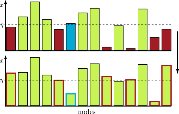
Figure 13: An illustration of the coherent noise mechanism. An external stress $\eta$ affects the nodes whose thresholds are smaller then $\eta$ (red, top diagram). The thresholds of the affected nodes are uniformly re-assigned (stroked red, bottom diagram). A small fraction of randomly drawn nodes (blue, top diagram) receives in addition a new, randomly selected, threshold (stroked blue, bottom diagram).

A dynamical system may organize itself towards criticality as the result of balancing competing driving forces, as discussed in the context of absorbing state transitions in Sect. 2.3. Generalizing this concept one can consider the effect of competing driving forces on the dynamics of the resulting state.

An interesting class of models with competing drives are random barrier models. An example is the Bak and Sneppen model [6], which is a model for co-evolutionary avalanches. In this model one has barriers $x_{i}\in[0,1]$ which represent obstacles to evolutionary changes. At every time step the lowest barrier is removed, corresponding to an evolutionary process of species $i$ and reset to a random value. The barriers $x_{j}$ of certain number of other species will also change and their barrier values will be reset randomly. The resulting state is critical and it can be related to a critical branching process [64] (see 4).

In the Bak and Sneppen model there are two competing driving forces, the removal of low barriers and the homogeneous redistribution of barrier levels. Another model with an equivalent set of driving forces, which we will now discuss briefly, has been termed “coherent noise model” [122]. The two steps of the time evolution, illustrated in Fig. 13, correspond to an external driving and an internal dissipative process respectively.

• All barriers below a randomly drawn stress level $\eta$ are removed and uniformly re-assigned (external forcing).

• A certain fraction $f\in[0,1]$ of barriers is removed anyhow and uniformly re-assigned (internal dissipation).

The coherent noise model has a functional degree of freedom, the distribution $\rho_{s}(\eta)$ for the stress levels, which is generally assumed to be monotonically decreasing, with low stress levels being more likely than larger ones. The distribution $p(x,t)$ of barrier levels $x\in[0,1]$ will reach a steady state, resulting from the competition of above two driving forces. The time evolution is given by

$$p(x,t+1) = \int_{0}^{1}\rho_{s}(\eta)p(x,t)\Theta(x-\eta)d\eta-fp(x,t)$$

$$+ \int_{0}^{1}dx\int_{0}^{1}\rho_{s}(\eta)p(x,t)\big{[}1-\Theta(x-\eta)\big{]}d\eta+f$$

where the terms in the second line enforce the conservation of the number of barriers, $\int p(x,t+1)dx=\int p(x,t)dx$, and where $\Theta$ is the Heaviside step function. The equilibrium barrier distribution $p(x)\equiv p(x,t)=p(x,t+1)$ is then given by

$$p(x)=\frac{c}{1+f-P_{s}(x)},\qquad\quad P_{s}(x)=\int_{0}^{x}\rho_{s}(\eta)\,d\eta\leavevmode\nobreak\ ,$$ (17)

where $c$ is an appropriate normalization constant. All barriers would pile up at the maximal barrier level in the absence of dissipation $f\to 0$. A non-trivial distribution results only when both external forcing and internal dissipation are active, the steady-state solution is structureless if only the internal redistribution of barriers $\propto f$ would be active, the reason why one can consider this process to be analogous to friction in physics. The steady-state barrier distribution (17) looks otherwise unsuspicious, not showing any obvious signs of criticality. A phase transition, and an eventual self-organization towards criticality, is in any case not expected for the coherent noise model due to the absence of agent-agent interactions. However, the resulting distribution of event sizes $s=\int_{0}^{\eta}p(x)dx$ shows an intermediate region of power-law scaling, and a large event is followed by a series of smaller aftershocks with power-law scaling [146].

The coherent noise model was used initially to describe the properties of mass extinctions observed in fossil records [119]. It was also considered as a model of earthquakes, describing the properties of aftershocks [164, 28], and used for the prediction of aftershocks [143]. Recently, Melatos and Warszawski [110] applied the coherent noise model in a study of pulsar glitches. Interestingly, the model is quite sensitive to initial conditions [51]; a property in common with the Bak-Sneppen model.

3.4 Highly optimized tolerance

The mechanism of highly optimized tolerance (HOT) is motivated by the fact that most complex systems, either biological or man-made, consist of many heterogeneous components, which often have a complex structure and behavior of their own [23]. Thus, real complex systems often exhibit self-dissimilarity of the internal structure rather then self-similarity, which would be expected if the self-organization toward a critical state would be the sole organizational principle [24, 25].

Self-similarity is a property of systems which have similar structures at different scales, a defining property of fractals. It is not uncommon to find fractal features in living organisms, in specific cells or tissue structures [162]. Self-similarity does however exist, for real-world systems, only within a finite range of scales. Cell shapes and functions differ substantially from one organ to another and there are highly specialized non-similar units within individual cells. Analogous statements can be made for the case of artificial systems, such as the Internet or computers. Actually, the diversity in the components of complex systems is needed to provide a robust performance in the presence of uncertainties, either arising from changes in the behavior of the system components or from changes in the environment. The balance between self-similarity and diversity hence comes not from a generic generating principle, but from the driving design process. Optimal design is achieved, for the case of living organisms, through natural selection and for the man-made complex systems, through human intervention.

Both man-made and biological complex systems can show a surprising sensitivity to unexpected small perturbations, if they had not been designed or evolved to deal with them. To give an example, the the network of Internet servers is very robust against the variations in internet traffic volume, nevertheless highly sensitive to bugs in the network software. Likewise, complex organisms may be highly robust with respect to environmental variations and yet may easily die if the regulatory mechanism, which maintains this robustness, is attacked and damaged by microscopic pathogens, toxins or injury. A substantial variety of complex systems is hence characterized by a property one may denote as “robust-yet-fragile” [23, 24, 25].

Carlson and Doyle [23] have argued, using simple models, that optimization of a design objective, in the presence of uncertainty and specified constrains, might lead to features such as high robustness and resilience to ”known” system failures, high sensitivity to design flaws and unanticipated perturbations, structured and self-dissimilar configurations, and heavy-tail distributions [45]. Depending on the specific objectives which are optimized, and their relation to the system constrains, the exact scaling can follow a power law or some other heavy-tailed distribution [25]. The main difference between the SOC and the HOT mechanism is their explanation of large, possibly catastrophic events. Large events arise, within SOC, as a consequence of random fluctuations which get amplified by chance. As for HOT, large events are caused by a design which favors small, frequent losses, having rather predictable statistics, over large losses resulting from rare perturbations.

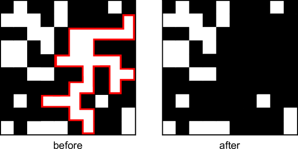
Figure 14: Illustration of a site percolation process on a $10\times 10$ regular lattice for $p=1/2$; occupied nodes are colored white. Before the perturbation targeting the largest cluster, which is shaded in red (left) and after the perturbation leading to the removal of all occupied nodes within the perturbed cluster (right).

3.4.1 HOT site percolation

The HOT mechanism can be illustrated with a model based on two dimensional site percolation [24]. This type of model is often taken as a starting point for describing the spreading of fire in forest patches or the spreading of epidemics through social cliques. It also serves, more generally, as a model for energy dissipation. Considering the reaction of the system under a disruption, one is interested in these cases in the number of trees surviving a fire outbreak, in the number of individuals unaffected by an epidemic, and in the amount of energy preserved within the system. For HOT one considers optimized percolation processes reducing to the classical Bernoulli percolation when no optimization is performed.

For the classical percolation problem, in the absence of any optimization procedure, lattice sites are occupied (with a particle, a tree, etc.) with probability $\rho$ and empty with probability $1-\rho$. Two sites are connected, on a square lattice with linear dimensions $L$ [24], if they are nearest neighbors of each others and a group of sites is connected whenever there is a path of nearest neighbors between all sites of the cluster (see Fig. 14). The cluster sizes are exponentially distributed if the average density $\rho$ of occupied nodes is below the critical density $\rho_{c}$. At criticality the characteristic cluster size diverges and the cluster size distribution follows a power law. For densities above criticality there is a finite probability of forming an infinite cluster covering a finite fraction of the system, even in the thermodynamic limit. The probability that a given occupied site is connected to an infinite cluster is the percolation order parameter $P_{\infty}(\rho)$, which is zero for $\rho\leq\rho_{c}$, and monotonically increasing from zero to one for $\rho>\rho_{c}$.

One now considers clusters of occupied sites to be subject to perturbations (e.g. a spark when considering forest fires) that are spatially distributed with probability $f(\vec{r})$. When a perturbation is initiated at the location $\vec{r}$ of the lattice, the perturbation spreads over the entire cluster containing the site originally targeted by the attack, changing the status of all sites of the cluster from occupied to unoccupied (the trees burn down), as illustrated in Fig. 14. On the other hand, if the perturbed site is empty, nothing happens. The system is most robust if, on average, as few sites as possible are affected by the perturbation. The aim of the optimization process is then to optimally distribute particles onto the lattice, for a given average density of occupied sites. One hence defines the yield $Y$ of the optimization process as the average fraction of sites surviving an attack. Optimization of the yield can be achieved, through an evolutionary process, by increasing continuously the density of particles.

• Starting with a configuration of $N_{p}$ particles one considers a number $D$ of possible states of $N_{p}+1$ particles generated by adding a single particle to the present state.

• One evaluates the yield $Y$ for all $D$ prospective new states by simulating disruptions, distributed by $f(\vec{r})$. The state with the highest yield is then selected.

The optimization parameter, for this algorithm, is in the range $0\leq D\leq(N-N_{p})$, where $D=0$ corresponds to no optimization, i.e. to classical percolation. Increasing the number $D$ of trial states will, in general, lead to an increase in performance.

Figure 15: Comparison between evolved HOT states and random percolation. (a) Yield vs. density in the case of random percolation and evolved lattice configuration. (b) Cumulative distribution of event sizes $C(s)$ at the point of maximum yield of the evolved lattice configuration (log-log plot), for the case of random percolation and for two evolved configurations. [Courtesy of J. Doyle [23].]

In Fig. 15 the yield $Y$ is shown as a function of the mean density $\rho$, both for the case of random percolation and for the state evolved through the HOT process. The yield peaks near the percolation threshold $\rho_{c}=1/2$, for random percolation, decreasing monotonically to zero for $\rho>\rho_{c}$, a behavior easily understood when considering the thermodynamic limit $L\rightarrow\infty$. In the thermodynamic limit there are two possible outcome for an perturbation. Either the perturbation hits, with probability $P_{\infty}(\rho)$, the infinite clusters, or, with probability $1-P_{\infty}(\rho)$, some other finite cluster or an empty site. In the first case a finite fraction $P_{\infty}(\rho)$ of occupied sites are removed, in the second case only an intensive number of sites:

$$Y(\rho)=P_{\infty}(\rho)(\rho-P_{\infty}(\rho))+(1-P_{\infty}(\rho))\rho=\rho-P_{\infty}^{2}(\rho)\leavevmode\nobreak\ ,$$ (18)

the yield is directly related to the order parameter when no optimization is performed. A yield close to the maximally achievable value $\rho$ can, on the other side, be achieved when performing optimization with an optimization parameter $D$ close to its maximal value. The resulting distribution of occupied sites is highly inhomogeneous, many small clusters arise in regions of high attack rates $f(\vec{r})$, regions with low disruption rates are, on the other side, characterized by a smaller number of large clusters. The HOT state reflects the properties of the distribution $f(\vec{r})$ and is hence highly sensitive to changes of $f(\vec{r})$. The distribution of clusters is, in contrast, translationally invariant in critical state $\rho=\rho_{c}$ when no optimization is performed, and independent from $f(\vec{r})$. This model of optimized percolation hence illustrates the “robust-yet-fragile” principle.

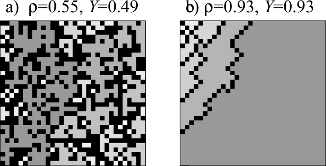
Figure 16: Sample of percolation configuration on a $32\times 32$ lattice for (a) random percolation near $\rho_{c}$ and (b) a HOT state at maximal yield obtained by evolving lattice configurations. Unoccupied sites are black and clusters are gray, with darker shades indicating larger clusters. The designed lattice percolation was generated for the perturbation probability $f(\vec{r})=f(r_{1})f(r_{2})$, where $f(x)=\exp(-\left(\frac{m_{x}+(x/N)}{\sigma_{x}}\right)^{2})$, which were peaked at the upper left corner of the lattice [Courtesy of J. Doyle [23]].

3.4.2 Fat tails and the generic HOT process

It is not evident, at first sight, why the procedure of highly optimized tolerance should lead to power-law scaling, or to fat tails in general. The emergence of power-law scaling from the HOT mechanism can however be understood by considering an abstract optimization setup as described by Carlson and Doyle [23]. The yield is defined as

$$Y(\rho)=\rho-\frac{1}{L^{2}}E[s],$$ (19)

where $E[s]$ denotes the expectation value of event sizes for a fixed distribution of perturbations $f(\vec{r})$. The yield $Y$ is maximal when a disruption triggers events of minimal sizes.

For the case of optimized percolation, discussed in the previous section, the event size $s$ was assumed to be identical to the area $A(\vec{r})$ affected by a disruption happening at $\vec{r}$. In a larger context one may be interested not to minimize directly the affected area $A$, but some importance measure $s$ of the event, with the relevance $s$ of a given event being a nonlinear function of the primary effect,

$$E[s]=\int f(\vec{r})s(\vec{r})\textrm{d}\vec{r},\qquad\quad s=\big{(}A(\vec{r})\big{)}^{\gamma}\leavevmode\nobreak\ ,$$ (20)

where a polynomial dependence $s=A^{\gamma}$ has been assumed, with $\gamma>0$. For the case of optimized percolation the yield $Y[\rho]$ is evaluated for fixed particle density $\rho$. More generally, one can consider a constraint function $R(\vec{r})$ such that

$$\int R(\vec{r})\textrm{d}\vec{r}=\kappa$$ (21)

needs to be kept constant. Available resources are finite, $\kappa<\infty$, and need to be utilized optimally. Real-world examples for resources are fire breaks preventing wildfires, routers and DNS servers preventing large failures of the Internet traffic and regulatory mechanisms preventing failure amplification in organisms. Allocating more resources to some location, to limit the size of events, will generically lead to a reduction in the size of the area affected by a disruption. One may thus assume that the area locally affected by an event is inversely related to the local density of resource allocation, that is, $A(\vec{r})=(R(\vec{r}))^{-\beta}$, with $\beta$ being a positive constant related to the dimensionality of the system.

The HOT state in this abstract system is obtained by minimizing the expected cost (Eq. (20)) subject to the constraint on available resources (Eq. (21)), together with $A=R^{-\beta}$. The optimal state is found by applying the variational principle and solving

$$\delta\int\Big{[}f(\vec{r})\big{(}R(\vec{r})\big{)}^{-\gamma\beta}-\lambda R(\vec{r})\Big{]}\textrm{d}\vec{r}\equiv 0\leavevmode\nobreak\ ,$$ (22)

where $\lambda$ is a Lagrange parameter. The variation, relative to all possible resource distributions $R(\vec{r})$, yields

$$f(\vec{x})\sim\big{(}R(\vec{x})\big{)}^{\gamma\beta+1}\sim\big{(}A(\vec{x})\big{)}^{-(\gamma+1/\beta)}\sim\big{(}A(\vec{x})\big{)}^{-\theta},\qquad\quad\theta=\gamma+1/\beta\leavevmode\nobreak\ .$$ (23)

This relation lead to $A\sim f^{-1/\theta}$, the larger the event probability $f$, the smaller the affected area $A$. The cumulative probability distribution $C(A)$ of observing an event which spreads over an area larger or equal than $A$, in the case of an optimal HOT state, becomes

$$C(A)=\int_{A(\vec{r})>A}f(\vec{r})\textrm{d}\vec{r}=\int_{f(\vec{r})<A^{-\gamma}}f(\vec{r})\textrm{d}\vec{r}\leavevmode\nobreak\ .$$ (24)

Although not all $f(\vec{r})$ will result in a scale-free scaling of event sizes, there is however a broad class of distributions leading to heavy tails in $C(A)$ and consequently in the distribution $P(A)$ of event areas. For example, in the one dimensional case an exponential, a Gaussian and a power-law distributed $f(r)$ result in a heavy-tailed distribution of events. One can show, in addition, that similar relations also hold for higher dimensional systems [23]. An example of a perturbation probability $f$ which does not result in heavy-tailed event sizes would be a uniform distribution or, alternatively, perturbations localized within a small finite region of the system.

The above discussion of the HOT principle does not take into account the fact that real-world complex systems are, most of the time, part of dynamical environments, and that perturbations acting on the system will therefore not be stationary, $f=f(\vec{r},t)$. The HOT principle can be generalized to the case of a time dependent distribution of disruptions $f(\vec{r},t)$. A system can still be close to an optimal state in a changing environment when constantly adapting to the changes and if the changes are sufficiently slow, that is, if a separation of time scales exists [174]. An adaptive HOT model was used by Zhou et al. [175] to explore different scenarios for evolution and extinction, such as the effects of different habitats on the phenotype traits of organisms, the effects of various mutation rates on adaptation, fitness and diversity, and competition between generalist and specialist organism. In spite of using a very abstract and simple notion of organisms and populations, these studies were successful in capturing many features observed in biological and ecological systems [176].

4 Branching processes

One speaks of an avalanche when a single event causes multiple subsequent events. Similar to a snowball rolling down a snowfield and creating other toppling snowballs. Avalanches will stop eventually, just as snowballs won’t trundle down the hill forever. At the level of the individual snowballs this corresponds to a branching process—a given snowball may stop rolling or nudge one or more downhill snowballs to start rolling. The theory of random branching processes captures such dynamics of cascading events. First, we will discuss the classical stochastic branching process and its relation to SOC, branching models are critical when on the average the number of snowballs is conserved. Second, we will discuss vertex routing models for which local conservation is deterministic.

4.1 Stochastic branching

A branching or multiplicative process is formally defined as a Markov chain of positive integer valued random variables $\{Z_{0},Z_{1},\ldots\}$. One of the earliest application of the branching processes concerned the modelling of the evolution of family names, an approach known as the Galton-Watson process [64]. In this context $Z_{n}$ corresponds to the number of individuals in the $n$th generation with the same family name. More recently, the theory of branching processes was applied in estimating the critical exponents of sandpile dynamics, both for regular lattices [3] and for scale-free networks [59]. In a typical application branching processes are considered as mean-field approximations to the sandpile dynamics, obtained by neglecting correlations in the avalanche behavior [171].

             

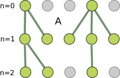
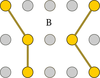
Figure 17: Examples for branching processes (A, left) and routing processes (B, right), where $n$ denotes a time step.

More abstractly, a random variable $Z_{n}$ represents the number of “particles” present at iteration step $n$ generating a new generation of $Z_{n+1}$ descendents at step $n+1$ (see Fig. 17). We denote with $p^{(n)}_{k}$ the probability that a single particle at time step $n$ generates $k$ offsprings at time step $n+1$ and with $P_{n}(Z_{n})$ the probability of finding $Z_{n}$ particles after $n$ iterations. One defines with

$$f_{n}(x)=\sum p^{(n)}_{k}x^{k},\qquad\quad G_{n}(x)=\sum_{Z_{n}}P_{n}(Z_{n})x^{Z_{n}}$$ (25)

the corresponding generating functions $f_{n}(x)$ and $G_{n}(x)$ [64]. A branching process may, in general, be time dependent, for a time-independent process $p^{(n)}_{k}\equiv p_{k}$ and $f_{n}(x)\equiv f(x)$. The recursion relation

$$G_{n}(x)=\sum_{Z_{n}}P_{n}(Z_{n})x^{Z_{n}}=\sum_{Z_{n-1}}P_{n-1}(Z_{n-1})\left(f_{n-1}(x)\right)^{Z_{n-1}}=G_{n-1}(f_{n-1}(x))$$ (26)

expresses the fact that branching processes are Markovian. When using branching processes to study properties of SOC systems we are interested in the scaling of the cumulative number of offsprings $s=\sum Z_{k}$, corresponding to the avalanche size (defined as the number of overall active sites), and in the duration $t$ of a branching process. An avalanche stops when no offsprings are produced anymore, hence when $Z_{t}>0$ and $Z_{t+1}=0$, which defines the duration $t$.

The probability of having no particles left after $n$ iterations is $q_{n}\equiv P_{n}(0)=G_{n}(0)$. One defines with $q=\lim_{n\rightarrow\infty}q_{n}$ the overall extinction probability; a finite probability exists, for $q<1$, of observing infinitely long and infinitely large branching events. The regime $q<1$ is termed supercritical, while the critical and subcritical regimes are found when the process extinction is certain, that is, $q=1$. The extinction probability is hence a convenient measure for characterizing the scaling regimes of branching processes.

The branching regimes are determined by the long term behavior of the average number of particles,

$$E[Z_{n}]=\sum_{Z_{n}}P_{n}(Z_{n})Z_{n}=G_{n}^{\prime}(1)\leavevmode\nobreak\ .$$

Defining with $\mu_{n}=\sum kp^{(n)}_{k}=f^{\prime}_{n}(1)$ the average number of offsprings generated by a single particle at time step $n$, one obtains the recursion relation

$$E[Z_{n}]=G_{n}^{\prime}(n)=f^{\prime}_{n-1}(1)G^{\prime}_{n-1}(1)=\mu_{n-1}E[Z_{n-1}]=\mu_{n-1}\mu_{n-2}\cdot\cdot\cdot\mu_{0}\leavevmode\nobreak\ ,$$ (27)

when starting with a single particle, $E[Z_{0}]=1$. Assuming that for large $n$ the expected number of particles scales as $E[Z_{n}]=e^{n\lambda}$, then for negative Lyapunov exponents $\lambda<0$ the expectation converges to zero, diverging on the other side for positive $\lambda>0$. Thus, $\lambda<0$ is defined a subcritical branching process and $\lambda>0$ the supercritical regime. The Lyapunov exponent is given, through the recursion relation (27), as

$$\lambda=\lim_{n\to\infty}\left(\frac{1}{n}\ln E[Z_{n}]\right)=\lim_{n\to\infty}\left(\frac{1}{n}\sum_{n=0}^{n-1}\ln\mu_{n}\right)\leavevmode\nobreak\ .$$ (28)

The branching process is critical for $\lambda=0$. For a time-independent branching process one has $f_{n}(x)=f(x)$ and a fixed average number of offsprings per particle, $\mu_{n}=\mu=f^{\prime}(1)$ for every $n$. Therefore, having $\mu=1$ and $\ln\mu=0$ at every iteration step is then a necessary condition for the branching process to be critical.

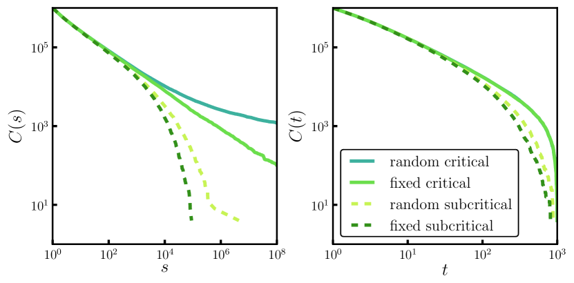
Figure 18: Comparison of the complementary cumulative distributions of sizes $s$ ($C(s)$, left) and durations $t$ ($C(t)$, right) for branching processes in fixed and random environments. The probability that a single particle generates $k$ offspring was set to a Poisson distribution $p_{k}=\mu_{n}^{k}e^{-\mu_{n}}/k!$. At each time step one sets $\mu_{n}=e^{X_{n}}$, where $X_{n}$ was drawn from a normal distribution $\mathcal{N}(\lambda,\sigma^{2})$, with $\lambda=0$ for the critical process, $\lambda=-0.01$ for the subcritical process, $\sigma=0$ for fixed environment and $\sigma=0.1$ for random environment.

Otter [124] has demonstrated that in the case of fixed environments and a Poisson generating function $f(x)$ the tails of the distributions $P(s)$ of avalanche sizes and durations $P(t)$ have the following scaling form:

$$P(s)\sim s^{-3/2}\mu^{s-1}e^{s(1-\mu)},\qquad\quad P(t)\sim t^{-2}\mu^{t-1}e^{t(1-\mu)}\leavevmode\nobreak\ .$$ (29)

The branching is critical for $\mu=1$, with the well-known scaling exponents $3/2$ and $2$ for the avalanche size and duration respectively.

The scaling behavior is more difficult to predict in the case of a changing or random environment. Consider an average number of offspring generated by a single particle which is given by $\mu_{n}=e^{X_{n}}$, where $X_{n}$ is drawn, at each time step, from some probability distribution $\rho(x)$. Again, the branching process is critical if $\lambda=0$, that is, if $E_{\rho}[x]=0$. Still, in contrast to fixed environment, the average number of particles $E[Z_{n}]$ fluctuates between infinity, $\lim_{n\rightarrow\infty}\sup\left(\ln E[Z_{n}]\right)=\infty$, and zero, $\lim_{n\rightarrow\infty}\inf\left(\ln E[Z_{n}]\right)=-\infty$, where the supremum and infimum are taken over ensemble realizations [159]. Furthermore, critical branching in random environments is a complex process and does not necessarily follow power-law scaling. Vatutin [159] has recently shown that, given a specific family of offspring generating function $f_{n}(x)$, the total size of the branching process has logarithmic correction whereas the duration distribution still follows a typical power-law scaling. In Fig. 18 we present a comparison of the scaling behavior of critical and subcritical branching processes in fixed and random environments.

When mapping a real-world phenomenon to a branching process, it is assumed that the phenomenon investigated propagates probabilistically. For example, when considering the propagation of activity on a finite network, each of the neighbors of an active node may be activated with some probability, say $p_{ij}$. Thus, the probability that the $i$th node will activate a certain number of neighboring nodes is given by the following generating function:

$$f^{(i)}(x)=\prod_{j=1}^{k_{i}}(1-p_{ij}+p_{ij}x)\leavevmode\nobreak\ ,$$ (30)

where the degree $k_{i}$ denotes the total number of neighbors of the $i$th node. On the average the $i$th node will activate $\mu^{(i)}=\sum_{j}p_{ij}$ neighbors. This branching dynamics leads to correlation effects due to loops in the network structure. In the simplest approximation one neglects correlation effects and the avalanche propagation will be critical when every site activates, on the average, one node, $\mu^{(i)}=1$. In Fig. 19 we present the critical scaling behavior of avalanche size and durations as we switch from the case when there is equal probability of activating any of the neighboring nodes ($p_{ij}=p_{i}=1/k$) to the case where the activation one of the neighbors ($p_{ij}\rightarrow 1$ when $j=j^{*}$ and $p_{ij}\rightarrow 0$ when $j\neq j^{*}$).

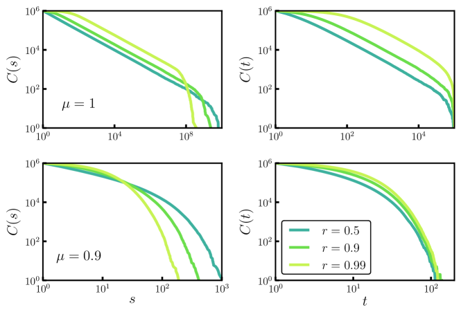
Figure 19: The complementary cumulative distribution of sizes $C(s)$, and durations $C(t)$, of avalanches of a critical and subcritical branching process on a $d=5$ dimensional lattice. The probability of activating a $j$th neighbor of the $i$th active node is given as $p_{ij}=\alpha r(1-r)^{k-1}$, where $\alpha=\mu/\sum_{k=1}^{k=2d}p_{ij}$. Thus, each active node on average activates $\mu$ neighbors. For critical branching (top) $\mu=1$, for subcritical branching (bottom) $\mu=0.9$ . Increasing $r$ leads to an increase in the probability of activating only the first neighbor, hence in the limit $r\rightarrow 1$ only one node is active in each time step, the process becomes deterministic.

This probabilistic description of branching process on a network is useful for mapping the behavior of a real-world phenomena, when the exact state of the whole physical system is unknown, that is when at any moment only a small subset of the complete system is studied. Even a deterministic process will appear stochastic if there are hidden, non-observable variables and dependencies of the current state on the exact history, viz if the process is non-Markovian. For example the activation of a network node may lead to the activation of the same set of nodes whenever the same activation history is repeated. Neglecting memory effects can lead to the conclusion that neighboring nodes are activated in probabilistic manner. Using a random branching process for modelling is, in this case, equivalent to an average of the observed activations, over sampled system states.

In the next section we will discuss the scaling behavior of a special case of branching processes, such that $\mu=1$ and $p_{ij}=1$ for some $j=j^{*}$. These conditions are satisfied when the activation of a single node leads with certainty to the activation of exactly one of its neighbors. We call this limiting case of a branching process a routing process [107].

4.2 Vertex routing models

A routing process can be considered as a specialization of random branching, see Fig. 17. For random branching the probability $p_{ij}$ of activating the $j$th neighboring node is equal for all neighbors, that is $p_{ij}=1/k_{i}$ for every $j=1,\ldots,k_{i}$, where the degree $k_{i}$ is the number of neighbors of the $i$th node. For a routing process, in contrast, only a single neighbor is activated. An example of a system exhibiting routing-type behavior is a winner-take-all neural network [62, 63], where at any time only a single neuron may be active, or, alternatively, only a single clique of neurons becomes active suppressing the activity of all other competing cliques [62]. One may also view routing processes as the routing of information packages and study in this context the notion of information centrality [107], which is defined as the number of information channels passing through a single node.

Here we discuss the relation of vertex routing to scaling in critical dynamical systems. Routing models are critical by construction with the routing process being conserved. The type of vertex routing models considered here are exactly solvable and allow to study an interesting question: Does the scaling of an intrinsic feature, e.g. of a certain property of the attractors, coincide with what an external observer would find when probing the system? Vertex routing models allow for a precise investigation of this issue and one finds that the process of observing a complex dynamical system may introduce a systematic bias alternating the resulting scaling behavior. For vertex routing models one finds that the observed scaling differs from the intrinsic scaling and that this disjunction has two roots. On one hand the observation is biased by the size of the basins of attraction and, on the other hand, the intrinsic attractor statistics is highly non-trivial in the sense that a relative small number of attractors dominates phase space, in spite of the existence of a very large number of small attractors.

4.2.1 Markovian and non-Markovian routing dynamics

We discuss here routing on complete networks, i.e. networks which are fully connected, and consider the routing process as the transmission of an information package, which may represent any preserved physical quantity. In general, routing of the information package to one of the neighboring nodes may depend on the routing history, that is, on the set of previously visited (activated) nodes. We denote with $m$ the depth of the routing memory retained. The routing is then Markovian if $m=0$ and non-Markovian otherwise. An illustration of a basic routing transition is presented in Fig. 20 for $m=0$ and $m=1$.

Let us denote with $v_{t}$ a node active at time step $t$, where $v_{t}\in V=\{1,\ldots,N\}$ with $N$ denoting the network size. Which of the $N-1$ neighbors of the node $v_{t}$ will become activated in the next time step $t+1$ will depend, through the transition probability $P(v_{t+1}=j|v_{t},\ldots,v_{t-m})=p_{j|v_{t},\ldots,v_{t-m}}\in\{0,1\}$, on the set of the $m$ previously visited nodes. The routing process is considered conserved whenever $\sum_{j}p_{j|v_{t},\ldots,v_{t-m}}=1$. For example, given some routing history in a network of $N=20$ nodes, say $v_{t}=3$, $v_{t-1}=4,\ \ldots,v_{t-m}=15$, there would be only one possible successor vertex, say $v_{t+1}=8$, and all other $N-1$ nodes would be unreachable, given the specified routing history.

          

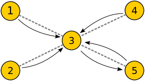
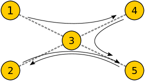
Figure 20: Examples of routing process. Left: For the Markovian case, $m=0$. An information package is always routed to vertex 5 independently of where it came from. Right: For a one-step memory, $m=1$. Information packages arriving at vertex 3 from the vertices 4 and 2 are routed to vertex 5, while packages arriving from vertex 1 and vertex 5 are routed to vertex 4 and 2 respectively.

A sequence of $m+1$ vertices can be seen as a point in the (enlarged) phase space of routing histories with $p_{j|v_{t},\ldots,v_{t-m}}$ defining the adjacency matrix on the directed graph of phase space elements. To give an example, a point $[v_{m+1},\ldots,v_{1}]$ of the enlarged phase space is connected to some other point $[v_{m+2},\ldots,v_{2}]$ if $P_{v_{m+2}|v_{m+1},\ldots,v_{1}}=1$, where $v_{i}\in V$. The volume of the enlarged phase space, given as the total number of containing elements, is $\Omega=NK^{m}$ where $K=N-1$, for the case of a fully connected network.

4.2.2 Intrinsic properties vs. external observation

One usually considers as “intrinsic” a property of a model when evaluated with quenched statistics, hence when all parameters, like connectivities, transition probabilities, etc., are selected initially and then kept constant [64]. An external observer has however no direct access to the internal properties of the system. An unbiased observer will try to sample phase space homogeneously and then follow the flow of the dynamics, evaluating the properties of the attractors discovered this way. Doing so, the likelihood to end up in a given attractor is proportional to the size of its basin of attraction. The dynamics of the observational process is equivalent to generate the transition matrix “on-the-fly”, viz to a random sampling of the routing table $p_{j|v_{t},\ldots,v_{t-m}}$. Both types of dynamics can be evaluated exactly for vertex routing models.

Intrinsic attractor statistics

We first consider quenched dynamics, the transition probabilities $p_{v_{t+1}|v_{t},\ldots,v_{t-m}}$ are fixed at the start and not selected during the simulation. A routing process initiated from a randomly selected point in phase space will eventually settle into a cyclic attractor. The ensemble averaged distribution of cycle lengths is obtained when using the set of all possible realizations of the routing tables, created by randomly selecting the values for the transition probability, $p_{v_{t+1}|v_{t},\ldots,v_{t-m}}\in\{0,1\}$, while maintaining following conditions

$$\sum_{v_{t+1}}p_{v_{t+1}|v_{t},\ldots,v_{t-m}}=1,\qquad\sum_{v_{t+1},v_{k<t+1}}p_{v_{t+1}|v_{t},\ldots,v_{t-m}}=K\leavevmode\nobreak\ ,$$

where $K=N-1$ is the coordination number. The average number of cycles of length $L$, when the routing is dependent on the $m$ previous time steps, and for a network with $N$ nodes, is given by [90, 108]

$$\langle C_{m}\rangle(L,N)=\frac{N}{LK}\frac{(K^{m+1})!}{K^{(m+1)(L-1-m)}(K^{m+1}+m+1-L)!}\leavevmode\nobreak\ .$$ (31)

The relation (31) is, for finite networks with $N<\infty$, an approximation for the non-Markovian case with $m>0$, as it does not take into account corrections from self intersecting cycles, i.e. cycles in which a given node of the network is visited more then once. Beck [9] studied this model for the Markovian case, in analogy to random maps, mainly in the context of simulating chaotic systems on finite precision CPUs (central processing unit of computer hardware).

		quenched	random
$m=1$	$\displaystyle\langle n\rangle$	$\log(N)$	–
	$\langle L\rangle$	$N/\log(N)$	$N$
$m=0$	$\langle n\rangle$	$\log(N)$	–
	$\langle L\rangle$	$\sqrt{N}/\log(N)$	$\sqrt{N}$

Table 3: Scaling with the number of vertices $N$, for the number of cycles $\langle n\rangle$ and for the mean cycle length $\langle L\rangle$ for history independent process ($m=0$) and the history dependent process ($m=1$), and for the two probing methods, quenched sampling and random sampling.

One can show that there is, in the limit of large networks, an equivalence between increasing the network size and increasing the memory dependence. This relation can be seen from the following memory dependent scaling relation

$$\langle C_{m+\tau}\rangle(L,N)\propto\langle C_{m}\rangle(L,N^{\prime}),\qquad\quad N^{\prime}\approx 1+(N-1)^{1+\frac{\tau}{m+1}}\leavevmode\nobreak\ ,$$ (32)

to leading order (for large $N$). Obviously, when $m=0$ we get $N^{\prime}-1\approx(N-1)^{\tau+1}$, thus each additional step of history dependence effectively increases exponentially the phase space volume. On the other hand, in the limit $m\rightarrow\infty$ we obtain $N^{\prime}=N$, any additional memory step in the system with already long history dependence will not drastically change the total number of cycles.

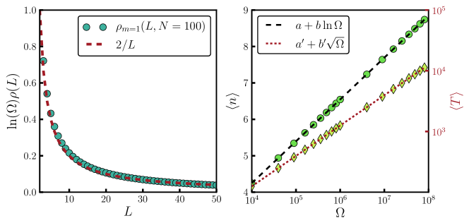
Figure 21: Left: The cycle length distributions $\rho_{m}(L,N)$, rescaled by $\log(\Omega)$, for the vertex routing model ($N$: network size, $L$ cycle length). The dashed line, $2/L$, represents the large-$N$ and small-$L$ limiting behavior. Right: As a function of phase space volume $\Omega$, the average total number of cycles $\langle n\rangle$ (circles, linear scale - left axis) and the expected total cycle length $\langle T\rangle$ (diamonds, logarithmic scale - right axis). The dashed line is fit using $a+b\ln\Omega$ ($a=-0.345(3)$, $b=0.4988(2)$), and the doted line a fit using $a^{\prime}+b^{\prime}\sqrt{\Omega}$ ($a^{\prime}=-0.3311(5)$, $b^{\prime}=1.25331\pm 2\cdot 10^{-7}$). The coefficient of determination is $R^{2}=1.0$ in both cases, within the numerical precision.

The analytic expression (31) for the cycle-length distribution can be evaluated numerically for very large network sizes $N$, or alternatively as a function of phase space volume $\Omega=NK^{m}$. The total number of cycles $\langle n_{m}\rangle(\Omega)=\sum_{L}\langle C_{m}\rangle(L,\Omega)$ present in the system shows logarithmic scaling as a function of the phase space volume $\Omega$, as shown in Fig. 21. The growth is hence slower than any polynomial of the number of vertices $N$, which is in contrast to critical Kauffman models, where it grows faster then any power of $N$ [47, 141]. A numerical evaluation of the total cycle length, defined as $\langle T_{m}\rangle_{\Omega}=\sum_{L}L\langle C_{m}\rangle_{\omega}(L)$, shows power-law scaling with phase space volume, namely as $\sim\sqrt{\Omega}$. Thus, the mean cycle length scales as

$$\langle L_{m}\rangle_{\Omega}=\frac{\langle T_{m}\rangle_{\omega}}{\langle n_{m}\rangle_{\Omega}}=\frac{a^{\prime}+b^{\prime}\sqrt{\Omega}}{a+b\ln\Omega}\leavevmode\nobreak\ ,$$ (33)

as shown in Fig. 22.

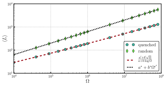
Figure 22: The mean cycle length $\langle L\rangle$ for the vertex routing with the quenched dynamics (blue circles) and the vertex routing with random sampling (green diamonds), as a function of the phase space volume $\Omega$; log-log plot. The dashed line is the fit of the form ${a^{\prime}+b^{\prime}\sqrt{\Omega}}/{a+b\ln\Omega}$, for the parameters see Fig. 21. The doted line is a fit of the form $a^{*}+b^{*}\Omega^{c^{*}}$, with $a^{*}=1.3319(3)$, $b^{*}=0.62666\pm 2\cdot 10^{-6}$, $c^{*}=0.5\pm 9\cdot 10^{-8}$. The coefficient of determination is $R^{2}=1.0$ in both cases, within the numerical precision.

The probability $\rho_{m}(L,N)$ of finding, for a network with $N$ nodes, an attractor with cycle length $L$ is obtained by normalizing the expression (31). One can show that the rescaled distribution $\log(\Omega)\rho_{m}(L,N)$ has the form $2e^{-L^{2}/2K^{m+1}}/L$, for small cycle lengths $L$, falling off like

$$\log(\Omega)\rho_{m}(L,N)\propto\frac{K^{(m+1)(M-\frac{1}{2})}}{M!}\leavevmode\nobreak\ ,$$ (34)

for large $L\rightarrow K\Omega/N+1$, where $M=K^{m+1}+1-L$.

Observed attractor statistics

Instead of considering quenched routing dynamics, one can sample stochastically the space of all possible realizations of routing dynamics [65]. In practice this means that at each time step one randomly selects the next element in the sequence of routing transitions. Algorithmically this is equivalent of starting at a random point in phase space and then following the flow. This is actually the very procedure carried out when probing a dynamical system from the outside. A cycle is found when previously visited phase space elements is visited for a second time.

Starting from a single element of phase space, the activation propagates until the trajectory reaches the same element for the second time. The probability of such a trajectory having a path length $s$, is given by

$$p_{s}=\frac{(s-1)(K^{m+1})!}{K^{(m+1)s)}(K^{m+1}-s+1)!}\leavevmode\nobreak\ .$$ (35)

In a path of length $s$, the observed cycle will have a length $L\leq s$. Thus, the joint probability of observing a cycle of length $L$ within a path of length $s$ is given by

$$p(L,s)=\frac{\Theta(s-L)\Theta(L-2)(K^{m+1})!}{K^{(m+1)s}(K^{m+1}-s+1)!}\leavevmode\nobreak\ ,$$ (36)

with $\Theta$ being the Heaviside step function. Finally, one obtains the probability $\tilde{\rho}_{m}(L,N)$ (with $\tilde{\rho}_{m}$ denoting random dynamics and $\rho_{m}$ quenched dynamics) of observing a cycle of length $L$ as a sum over all possible path lengths, that is

$$\tilde{\rho}_{m}(L,N)=\Theta(L-2)\sum_{s=L}^{K^{m+1}+1}\frac{(K^{m+1})!}{K^{(m+1)s}(K^{m+1}-s+1)!}\leavevmode\nobreak\ .$$ (37)

Interestingly, the mean cycle length scales as $\sqrt{\Omega}$ when using random sampling as a method for probing the system of routing transition elements. The comparison of the respective scaling behaviors, as a function of the network size and for $m=0,1$, is given in Table 3. There are two implications [65].

• The results for the vertex routing model indicate that one needs to account for the procedure used to probe the scaling behavior of a complex system.

• Certain properties of critical dynamical systems, like the number of attractors, may not show power-law scaling, even at criticality.

Vertex routing models and random boolean networks are, furthermore, in different classes. The scaling relations shown in Table 3 do not translate into the ones for the Kauffman net [47, 141] when rescaling the dependence of the phase space volume $\Omega$ from $N(N-1)$ (valid for the $m=1$ routing model) to $2^{N}$, as valid for the Kauffman net.

5 Modelling experimental data

A mathematical model of real-world phenomena should both replicate the phenomena and capture the structure and the function of the described physical system. One may divide theory models as “descriptive” or “explanatory” [165]. A descriptive model tries to reproduce the statistical properties of the phenomena in question, while containing often unrealistic and simplistic assumptions about the structure of the modeled system. Thus, not attempting to explain the underlying generative mechanism of the phenomena of interest. In contrast, an explanatory model would reproduce both the phenomena while capturing the known structural and functional properties of the system modeled. It is, however, difficult to actually prove that a given model is “correct”. When modeling systems which are very complex, one has necessarily to resort to some simplifying assumptions and to neglect certain experimental aspects seen as secondary; and to concentrate on the primary aspect on interest, e.g. the power-law scaling of certain observables. Our discussion here will hence not be able to give definite answers. Willinger et al. [165] has pointed out in this context, that although descriptive models may provide an initial description for the possible causes of the phenomenon studied, a correct prediction of the dynamical behavior would require a consistent explanatory model for which the various assumptions incorporated into the model have been verified. Thus, we would like to understand whether SOC models provide an adequate explanatory description for various real-world phenomena and, if not, which extensions of current models are required or what would be an alternative explanatory model.

In the following sections we will give a short review of the some of the known statistical properties of the empirical time series of earthquake magnitudes, solar flares intensities and sizes of neuronal avalanches and compare experimental avalanche statistics with theory predictions, mostly for dissipative SOC models. We will also point out plausible alternative mechanisms leading to power-law scaling of event sizes without requiring a critical regime.

5.1 Earthquakes and Solar flares

Solar flares are large energy releases on the surface of the Sun and they are observed as a sudden brightening of a region on Sun’s surface. As the distribution of peak intensities of solar flares follows a power-law scaling, Lu and Hamilton [102] proposed SOC for a generative mechanism of flares in the solar corona. Looking at the total flare energy, which represents the size of an avalanche $s$, one finds that it follows a power-law scaling with an exponent $\tau_{s}\in[1.6,1.75]$ [33, 32].

Similarly, Sornette and Sornette [147] have initially suggested that the scaling behavior of earthquakes magnitudes would correspond to that of the SOC systems, a proposition motivated by the well known Gutenberg-Richter and Omori laws. The Omori law describes the empirical evidence that the frequency $f(t)$ of earthquake aftershocks decays, as function of time $t$ passed since the earthquake, as $1/t$, whereas the Gutenberg-Richter law states that the probability of observing an earthquake of magnitude of at least $M$ scales as $10^{-bM}$, where $b$ is a positive constant. The size of an avalanche $s$ is taken to be proportional to the scalar seismic moment, and its relation to the earthquake magnitude as $M=\frac{3}{2}\log_{10}(s)$ [83]. Hence, the probability $P(s)$ of finding an event of size $s$ follows a power-law scaling, that is $P(s)\sim s^{-\tau_{s}}$. The scaling exponent $\tau_{s}$ falls in the range $[1.6,1.7]$, independent of the region and of the depth of the earthquakes [83, 32], with values closer to the mean field prediction of $\tau_{s}=3/2$ also being discussed [84]. Note, that similar scaling laws are also observed in the scaling properties of solar flares, suggesting a common interpretation of these two phenomena [38].

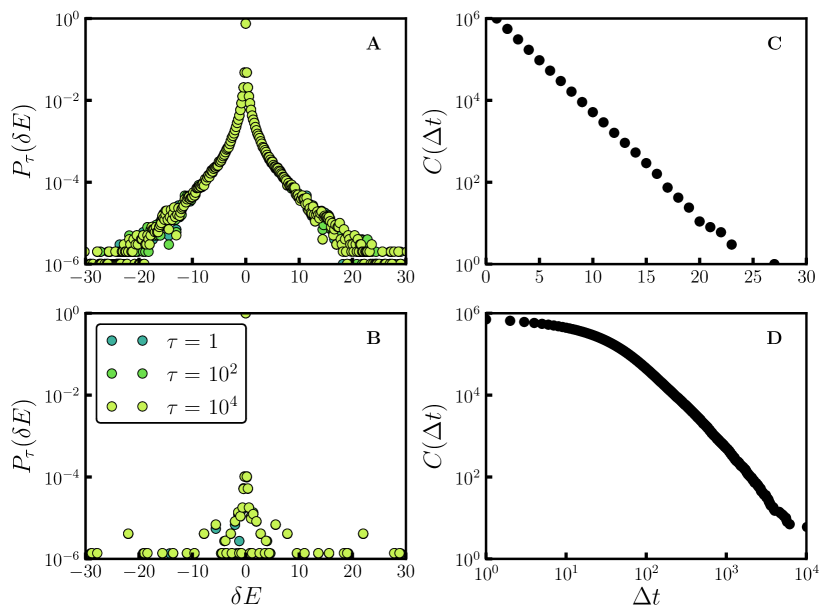
Figure 23: Probability distributions for released energy fluctuations $P_{\tau}(\delta E)$ (see Eq.38), obtained from (A) the avalanches generated by the BTW sandpile model (see Sect. 2), (B) the data set of earthquakes in North California in a period 1968 - 2012 (earthquakes of magnitude $M\geq 1$ in the NCEDC Earthquake Catalog). Overlapping data for various inter-event time scales $\tau$ indicate self-similarity. The respective CCDF (complementary cumulative probability distributions) of waiting times estimated (C) from the time series generated by the BTW sandpile mode and (D) from the time series of earthquakes.

The statistics of the released energy fluctuations, or the so called “returns”, is an important quantity characterizing self-similarity of a stochastic process, and a good yardstick for controlling the quality of modeling efforts. The quantity

$$\delta E=\frac{s(t+\tau)-s(t)}{\sigma_{\tau}},\qquad\quad\sigma_{\tau}^{2}=\left\langle(s(t+\tau)-s(t))^{2}\right\rangle$$ (38)

corresponds to the relative difference in the size of avalanches released at times $t$ and $t+\tau$ respectively. One may evaluate, for a fixed inter-avalanche time $\tau$, the distribution $P_{\tau}(\delta E)$ measuring the probability of finding an fluctuation $\delta E$ in the released energy.

Real-world and SOC avalanches may differ with respect to the statistics of the returns. The distribution $P_{\tau}(\delta E)$ is invariant with respect to a change of the time scale $\tau$, for classical SOC systems, that is, $P_{\tau}(\delta E)=P_{\tau^{\prime}}(\delta E)$ for any $\tau^{\prime}\neq\tau$. Experimentally observed energy fluctuations change—in the case of turbulent phenomena—with the inter-event time scale $\tau$, exhibiting multifractal scaling [21]. This observation led to the conclusion that classical SOC models cannot produce the higher order statistics typical for turbulent flows, which are however captured properly by models describing the energy cascades in turbulence [14, 54]. For the case of earthquakes, interestingly though, Caruso et al. [27] pointed out that the distribution $P_{\tau}(\delta E)$ of energy fluctuations is independent on the scale $\tau$, thus the time series is self-similar, as shown in Fig. 23.

Another important quantity for characterizing a time series of experimentally observed events is the waiting time distribution (WTD); the distribution of durations of quiet periods between events. The WTD observed for earthquakes and solar flares differs markably from the one produced by classical SOC systems, with the empirical time series showing a power-law distributed WTD and with the SOC waiting time distribution closely following an exponential distribution, as typical for a Poisson process charactering a memoryless time series [14, 54, 167, 35, 163]. Sánchez et al. [142] demonstrated that a modified sandpile model can produce a scale-invariant WTD, and multifractal scaling for the energy fluctuations. In addition, Paczuski et al. [125] showed, that the WTD follows a power-law when one considers the time scale of avalanches instead of the time scale of the external drive and putting a threshold to the minimal recorded intensity, at any point in time. Setting a signal threshold is an usual experimental procedure to distinguish between small events and background noise. Furthermore, Sattin and Baiesi [144] demonstrated that one obtains, when the external drive is spatially correlated, both power-law scaling for the WTD and multifractal scaling for the energy fluctuations [144, 30]. Thus, certain constrains to the driving force in SOC theories can generate some of the behavior observed in the empirical data.

Nevertheless, some concerns remain. When predicting the occurrence of an event of a certain size the distribution of waiting times is not as important as the correlations between waiting times. The predictability of a time series can be quantified by estimating the index of long-range time dependence, also known as the Hurst exponent $H$ [140]. For $H=1/2$ the time series is uncorrelated and unpredictable; this is exactly the value of the Hurst exponent obtained in different SOC models [27]—even in the presence of spatial correlation in the external driving force. In contrast, the estimates for the Hurst exponent for the time series of earthquakes and solar flares indicate the presence of a long-term memory in the empirical data [97, 125], that is, $H\in(1/2,1]$. These long-term correlations suggest that large events are more likely to be followed by events of similar or larger magnitude, possibly allowing for the prediction of intense events. For example, specific patterns have been observed in the seismic activity data preceding the main event, thus opening a venue for predicting large earthquakes [52, 79, 106].

Jagla [76] introduced a modified OFC earthquake model, see Sect. 2.5, and proposed a solution for this inconsistency between theoretical and experimental results. The modifications to the original OFC model consist of implementing structural relaxation and random threshold values for each node of the lattice—resembling the spatial inhomogeneity of real earthquake faults [86]. The relaxation mechanism equalizes the stress levels among neighboring nodes and works on the time scales of the driving forces—essentially infinitely slower then the time scale of avalanche topplings. The avalanches generated by this model follow a power-law scaling, with exponents independent on the dissipation levels; unlike the standard OFC model with inhomogeneities (see 2.5). Furthermore, the simulated time series is spatially and temporally correlated and exhibits patterns of aftershocks like the one observed in earthquakes and solar flares. Aftershocks are triggered by the relaxation mechanism after the main shocks—initiated by the external drive—due to the non-uniform distribution of thresholds.

A few questions still remain. Is this modified OFC model robust in the presence of non-uniform interactions between neighboring nodes [172]? Is the modified OFC model robust in the presence of complex network structures? An interesting issue since there are indications that the underlying network of earthquake epicenters has scale-free and small world structure [4, 1]. Finally, is the mechanism of structural relaxations universally applicable to other physical systems that show SOC dynamics or are system specific modifications required? If the required modifications to dissipative SOC models—in the presence of inhomogeneities—are system specific then the SOC behavior would start to depend on the exact dynamical constrains and local interaction rules, thus the universal properties of such regimes would be lost.

5.1.1 Tuned versus self-organized criticality

When studying naturally occurring phenomena, like solar flares and earthquakes, one cannot control experimental conditions and their effect on the behavior of the system. Small-scale experimental studies of power-law phenomena [169], in which the experimental conditions are carefully controlled, might provide important insights for our understanding of the power-law behavior observed in their large-scale counterparts.

Friedman et al. [56] analyzed the scaling behavior of fractures in metallic nanocrystals induced by an externally applied, slowly increasing, stress. A fracture or a slip occurs when the local stress level, within the crystal, exceeds the local threshold stress, with the slips generated by the fast release of pinned deformations. The process stops when the loose segments get repinned or annihilated, thus forming an avalanche. The avalanches are typically of length scales which are large with respect to the microscopic length scales. The distributions of slip sizes $s$, measured in different materials, follow a power-law , $P(s)\sim s^{-1.5}$, over several orders of magnitude and fall on a same scaling function. Interestingly, the size of the largest expected event $s_{max}$ scales with the strength of the externally induced stress $f$, as $s_{max}(f)=(f_{c}-f)^{-2}$, which diverges only for $f=f_{c}$ [170, 56]. The results for the statistics of slip-avalanches in nanocrystals obtained by Friedman et al. [56] have been analyzed within a molecular-field approximation for a micromechanical model for deformations in solids [34]. Within this model there is a second-order phase transition between brittle and hardening crystals (becoming respectively more/less susceptible to stress in the wake of a slip), thus scale-free avalanche statistics is observed.

In contrast, within SOC framework, the maximal size of an avalanche $s_{max}$ depends only on the system size and diverges in the thermodynamic limit independent on the other system parameters. Thus, to relate critical like behavior to a SOC or SOqC mechanism, one should demonstrate that no other parameters except system size influence the scaling. In other words, one should exclude tuned criticality as possible explanation. For example, the power-law scaling of earthquakes might be caused by near-critical stress levels in earth crust, which are just a transient state typical for the current geological era and not an attracting state, as would be the case in self-organized critical process. Unfortunately, this kind of hypothesis is difficult to test, as one cannot control the environmental parameters generating the earthquakes.

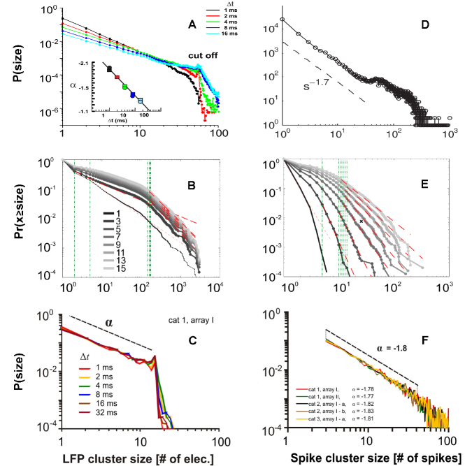
Figure 24: Distribution of sizes of neuronal avalanches estimated from the LFPs (left column) and from neural spike recordings (right column). (A) (adapted from Beggs and Plenz [12]) and (D) (adapted from Friedman et al. [55]) show the data obtained from in vitro recordings in acute slices and organotypic cultures. Examples of data obtained from in vivo neural activity in humans (B,E) (adapted from Dehghani et al. [40]) and cats (C,F) (adapted from Hahn et al. [67]).

5.2 Neuronal avalanches

Neuronal avalanches are sequences of bursts of neural activity which, separated by quiet periods, spread across the neural tissue. Since the introduction of SOC theory it has been hypothesized that the brain operates in the critical dynamical regime, as many features of neural spiking activity resemble the properties of sandpile models, namely the sudden release of energy (action potential) and the transmission of released energy to neighboring nodes (interaction of neurons mediated by neurotransmitters or ion diffusion). One of the first experimental evidences supporting this hypothesis was given by Beggs and Plenz [12]. They investigated the spontaneous neural activity measured in organotypic cultures (tissue which, removed from an organ, continues to develop as it would have done in the body) and in acute slices of rat cortex, observing power-law scaling of neuronal avalanches as extracted from the recordings of local field potentials. Similar evidences were later obtained from in vivo neural activity in humans [138], monkeys [128], cats [67] and also from high-resolution data measured in cultured slices of cortical tissue extracted from living rats [55]. In Fig. 24 we presented the distribution of sizes of neuronal avalanches adapted from various studies.

A local field potential (LFP) represents the recorded voltage generated by the sum of all currents on the surface of the small electrode embedded within the neuronal tissue. These currents reflect the dendritic activity within a small volume surrounding the electrode. The neuronal avalanches are constructed from the sequence of negative peaks of the LFPs propagating across multiple electrodes, because negative voltage peaks are correlated to synchronized spiking activity of nearby neurons [12, 87]. To distinguish between the troughs of LFPs from the troughs generated by the background noise, one has to define a threshold value for the recorded voltage. Only signals dropping below the threshold are considered in the definition of an avalanche. One calls an electrode active if the value of LFP on that electrode is below the threshold value. After identifying the relevant signals, the data is divided into time bins and the neuronal avalanche is defined as the sequence of recorded activity. An avalanche starts when at least a single electrode is active and ends when the signal is below threshold on all electrodes for at least one time bin. The avalanche duration is determined as the elapsed time between the first and the last bin; the size of the avalanche can be chosen either as the total number of active electrodes or as the absolute sum of LFP amplitudes over all active electrodes during the avalanche duration.

Beggs and Plenz [12] found that the avalanche size follows a power law with exponent close to $-3/2$ (see Fig. 24 A), with the avalanche duration following a power law with an exponent close to $-2$. These values for the critical exponents are, interestingly, identical with the mean-field results for critical branching processes in fixed environments (see Sect. 4). Note that the experimentally observed scaling behavior, thus the values of the exponents, of the neuronal avalanches will depend on the choice of the threshold value and on the selected width of the time bins [134]. Still, these values can be fixed if one takes into account certain properties of white noise signals and the propagation speed of action potentials along the neural cell membrane [12].

The initial work of Beggs and Plenz [12] lacked rigorous statistical estimates of the scaling laws, the confirmation of similar scaling behavior for in vivo recording, and evidence for a critical state going beyond the distribution of avalanche sizes and the $1/f$ scaling of the power spectrum (both necessary signatures for a critical state). A consensus on the dynamical state of neural activity is still missing even with experiments repeated and a refined data analysis including the previously missing factors. A central problem is the recording of neural activity in vivo with sufficiently high resolution, and the variations of the statistical properties of recorded activity between subjects and species [128, 133].

Touboul and Destexhe [157] showed, in a study performed on awake cats, for which the LPFs were measured with 8 channel multi-electrode arrays, that an exponential distribution is a better fit to the avalanche size distribution then a power-law distribution. Dehghani et al. [40] reached a similar conclusion by analyzing avalanches from recordings from the cerebral cortex of cat, monkey and human, both made during wakefulness and during sleep (See Fig. 24 B and E). He concluded that the optimal fit of the avalanche distributions is actually a double-exponential distribution. In contrast to the studies of Touboul and Destexhe [157] and Dehghani et al. [40], several investigations found evidence for power-law distributed neuronal avalanches. Petermann et al. [128] argued for scale invariant features of the cortical activity recorded from awake monkeys. Similarly, Klaus et al. [89] recently showed that a power law is the best fit for the neuronal avalanches recorded both in vivo and in vitro.

One of the possible explanation, for these opposing experimental results, may be traced back to the small number of recording electrodes used in some experiments, which may lead to a sub-sampling of the local neural activity. Priesemann et al. [133] argued that critical processes can appear subcritical in the scaling behavior if the activity is averaged over a small number of recording elements, relatively to the total number of elements which are actually generating the critical phenomena. Still, one should note that the analysis of peaks in LFP signals is an rather indirect measure of the neural activity patterns. Touboul and Destexhe [157] argued that simple thresholding of a stochastic process can generate an apparent power-law behavior, and that the use of LFP recordings for identifying the scaling properties of neuronal avalanches may hence be problematic. Furthermore, if one takes the positive peaks of the LFP signal, which are not related to spiking activity, instead of the negative peaks, applying the same procedure to estimate neural avalanches, one finds similar scaling behavior as for the negative peaks. Thus, Touboul and Destexhe [157] and Dehghani et al. [40] proposed that the observed scaling behavior may be a consequence of a thresholding procedure, and not a reflection of an underlying critical or near critical state. They stressed the point that one should investigate the scaling behavior of the avalanches estimated both from the negative and from the positive LFP peaks, with criticality being of possible relevance only if the respective scaling behaviors would differ qualitatively.

Beside estimating neuronal avalanches indirectly from the propagation of LFPs, one can also directly record neural spikes. For example, Hahn et al. [67] recorded spontaneous neural activity of adult cats under anesthesia and beside LFPs they also measured neural spikes. For both cases, they’ve found evidence of power-law distributed neuronal avalanches (see C and F subplots of Fig. 24). Also, Ribeiro et al. [138], observed power-law distributed neuronal avalanches recorded from the cerebral cortex and from the hippocampus of rats; in awake, asleep and anesthetized animals. These results are puzzling as one would expect sleep and awake states to be characterized by distinct dynamical regimes and by different responses to external stimuli [93]. Nevertheless, controversy persist even regarding the direct measurements of spiking activity, as Dehghani et al. [40] reported absence of power-law distributed avalanches.

In a recent study, where they recorded neural spikes in cultured cortical slices with high density multi-electrode arrays, Friedman et al. [55] showed that the average shapes of neuronal avalanches of different durations collapse to a single curve under an appropriate scaling transform, a strong evidence for a critical regime which even allows for the determination and the comparison of the dynamical universality class [91]. Interestingly though, out of ten samples of organotypic cultures used in this study, only two of them showed clear evidence for critical neuronal avalanches (see Fig. 24 D). The other samples showed subcritical or supercritical behavior. This suggest, that self-organization of cortical networks to a critical state may not be a generic property, but that it might depend on environmental conditions, on the interaction between different mechanisms of neural plasticity or on the current functional properties of global brain networks [134].

5.2.1 The origins of neuronal power laws

The underlying causes for the observed neural power laws are still under debate. On the experimental side, to give an example, the $1/f$ scaling of the power spectrum of the recorded LFPs could be ascribed to biophysical filtering effects of the extracellular media on the recorded signal [11, 10, 49]. Touboul and Destexhe [157] noted, in addition, that power-law scaling of peak events may arise from a thresholded stochastic process, a plausible model for the generic neural dynamics, which is however devoid of any connection to criticality or self-organization.

A basic precondition for the brain to retain functionality is, in agreement with experimental results, that the level of the average cortical activity remains within a certain range, neither exploding over time nor dying out. Mapping bounded neural dynamics to a branching process hence cannot result in neither a subcritical (with the neural activity becoming eventually extinct) nor in a supercritical (with an exploding neural activity) regime. This line of argument is valid if the majority of neural activity studied is stimulated internally and not induced by external sensory inputs. This is the case for the upper cortical layers, which are responsible for the intra-cortical communication. Interestingly, these upper cortical layers are also mostly the ones for which evidence for neuronal avalanches has been reported, together with a critical branching ratio [131].

A support for the SOC causes of neuronal avalanches comes from several theoretical studies using networks of spiking neurons. These artificial neural networks are related to dissipative SOC models and as such require a fine tuning of the external drive, which initiates the neuronal spikes, relative to the number of neurons in the network [17]. Nevertheless, one can still consider dissipative models as very close approximations to true SOC behavior observed in conserved sandpile models, as discussed in section 2. More importantly, these neural network models, although replicating very closely the experimentally observed statistical properties of neuronal avalanches, achieve critical behavior only for networks consisting of purely excitatory neurons [98] and the introduction of biologically realistic levels of inhibition breaks the power-law scaling of neuronal avalanches [113, 36]. The experimental observations [12] indicates that a network of excitatory neurons operates in a supercritical regime, which allows for a fast transfer of information, whereas inhibition has the role of stopping large neuronal avalanches and to localize information processing. Rather then spontaneously emerging from separation of time scales between external driving and internal dissipative mechanisms, the critical behavior in cortical networks seems to be reached through various plasticity mechanisms, whenever such a dynamical regime is optimal for given environmental conditions. This kind of reasoning is closer to the HOT theory (see Sect. 3.4), which states that power-law scaling emerges through design aimed at optimal functioning in uncertain environments. For the case of the brain, and in general for entire organisms, this design is thought to emerge through natural selection.

Finally, in order to understand why a critical behavior of neuronal avalanches may be computationally favorable, and hence be selected through Darwinian evolution, one should look for the conditions under which the critical state may constitute an optimal working regime. An analysis of information retention and information transmission in simple models of branching processes on complex networks has shown that critical regimes offer certain advantages, when considering the computational performance of the network [131]. Beggs and Plenz [12] showed that the information transmission between input and output layers of a network is maximal in the critical branching regime, whereas Haldeman and Beggs [68] found that the critical state is optimal for information retention. Also, Kinouchi and Copelli [88] demonstrated that the critical regime is related to a maximal sensitivity of a neural network to the variations in the input activity. This interesting characteristic of the critical regime may be explained by fact that the dynamical regime at the border of a second-order phase transition shares in part the properties of the two phases. The activity in the frozen state would be, in this view, related to nonlinear computations with the activity in the chaotic state favorable for fast information transmission and parallelization of computational processes [139]. Thus, it is plausible that cortical areas organize into distinct dynamical states, depending on the required functionality; the critical regime might be an attracting dynamical state for computations needing the features of both states, that is, a large flexibility in information processing. Still, it is important to extend this simple models in a way which captures neural variability, adaptability and evolutionary design in order to reevaluate the hypothesis discussed above in biologically realistic setups.

5.3 Beyond power laws - dragon kings

We will conclude this section with a short discussion of the emerging topic of ”life beyond power laws”, which deals with an intriguing perspective regarding the possible origins of large catastrophic events. Sornette [149] and Sornette and Ouillon [153] pointed out that there is growing evidence indicating that extremely large events often transcend the heavy-tailed scaling regularly observed by the bulk of the data sets. These outliers were named ”dragon kings”, in order to stress their unique and diverse generating mechanisms, and their extreme size, which is typically off the charts.

The generating mechanisms of dragon kings are believed to differ from the ones generating the smaller events, such as the various mechanisms discussed in this review. Furthermore, they are diverse and system dependent, having however several common properties. For a dragon king to emerge an additional amplification mechanism is required, a mechanism which may not be present at all times in the system. The system then undergoes a temporary phase transition, or bifurcation, leading to a qualitative new state and possibly to large-scale events. These kinds of transitions may be caused by a sudden increase in coupling strength of interacting components, leading to increased positive feedback, and possibly to a synchronized regime, spanning across a large fraction of the system [153]. Interestingly, certain precursors typically precede a dragon king event, thus predicting an incoming catastrophe may be possible in certain cases. Johansen and Sornette [80] used the existence of a log-periodic precursors as an indicator for an impending material failure, and Sornette and Johansen [152] applied similar methods for the prediction of bursts of financial bubbles, that is, market crashes.

Dragon kings are rare events, although more frequent then what would be expected when using only the distribution of smaller events as a reference. Unfortunately, these features make them difficult to identify and to differentiate between dragon kings and a regular large-scale events. Tools and methods used for the identification of dragon kings often depend on the particularities of the system in question [149, 153]. Only recently had Pisarenko and Sornette [130] proposed a robust statistical test able to identify anomalies in the tails of power-law or exponential distributions, even when only a few dozens of observations are available.

Evidences for the existence of dragon kings have been found in numerous phenomena, such as various extreme weather phenomena, material rupture events, the distributions of financial runs of losses, in the statistics of epileptic seizures in humans and animal models, and many others [149, 153]. Still, in several cases the evidence of the dragon kings existence is inconclusive [153]. For example, it is still debated whether genuine dragon kings exist in the distribution of earthquake magnitudes.

6 Conclusions

The concept of self-organized criticality (SOC) is an intensely studied and discussed mechanism for generating power-law distributed quantities. This theory has been proposed as an explanation for power-law scaling observed in various real-world phenomena. We have focused here on several well-studied phenomena, notably earthquakes, solar flares, and neuronal avalanches; just a three out of a plethora of phenomena exhibiting fat tails. Given the amount of existing empirical data, it is important to understand to which extent the theory of SOC contributes to an understanding of the underlying causes of the observed power-law behavior in real-world complex dynamical systems.

The current experimental evidence is still inconclusive with respect to a possible causal relation of the emergent power laws to an underlying self-organized critical state. In any case, extensions of the original sandpile model, such as dissipative models like the OFC earthquake model, are essential for replicating the fat-tailed avalanche statistics which are temporally and spatially correlated, a key property of many real-world data sets. Furthermore, a satisfactory description for real-world systems would also need to account for the observed inter-event correlations, which by themselves are key to improved predictions of catastrophic events.

An alternative for an underlying self-organized critical state is the concept of highly organized tolerance (HOT), which does not require a critical dynamical state for generating distributions with heavy tails. The theory of HOT proposes an explanation for the emergence of scale invariance in artificial and natural systems as a consequence of system design, where the design aims to achieve an optimized and robust performance in uncertain environments. For the case of living organisms this robust design may plausibly emerge through natural selection, and also result as such from a self-organizing process, albeit on longer time scales.

In this context, an interesting and hitherto open research question regards the relation between self-organization and criticality in general. Essentially all proposed models for generating scale-invariant observables are based on self-organizing processes, some of which lead to critical states, while others do not. For example, any dynamical system, which retains its average activity homeostatically within certain bounds, as it is done in various cortical areas, is statistically equivalent to a self-organized critical branching process, and hence scale invariant. Balancing different types of drives, such as external driving and internal dissipation, may lead, on the other hand, to a self-organized, non-critical and heavy-tailed state, a route proposed by the coherent noise model.

A further complication concerning this discussion is added by the circumstance that critical dynamical systems may not actually be intrinsically scale invariant, which is in contrast to thermodynamic critical systems. We discussed property in the context of vertex routing models. Another important aspect regards the process of probing a complex dynamical system, which is normally done by a stochastic sampling of phase space and then following the dynamical flow. The measurement process may actually have a qualitative effect on the resulting scaling properties of observables, an effect which has been worked out in detail for the case of vertex routing models. Both effects can be traced back to a highly non-trivial statistics of the attractors which might emerge in a critical dynamical system.

On the experimental side, power-law regimes are routinely observed in both physical and biological systems. Considering the functional aspect, critical dynamical states have been argued to be advantageous for non-linear sensory processing and self-sustained neural computation [116], which are crucial characteristic biological neural networks. Living organisms are the product of self-organizing processes and it is therefore likely – considering the functional advantages of critical regimes – that the observed heavy-tailed distributions will result from self-organizing principles. The SOC mechanism would imply that an underlying critical state, if realized, would be based on a very specific generating mechanism namely the separation of time scales between a fast internal dissipation (which may occur either at the boundary, for conserved sandpile models, or locally, for dissipative SOC models) and a slow external driving, as exemplified by absorbing state transitions. It may, however, also be the case that the underlying state is non-critical and is either the product of various regulatory mechanisms (like homeostatic plasticity), as proposed within the HOT theory, or the result of balancing external driving and internal dissipation occurring on similar time scales, as within the coherent noise model.

An important aspect regards the modeling of experimental data. Estimating the dynamical state of an avalanche-like phenomenon, such as neuronal avalanches, by mapping it to a branching process, to obtain an estimate of the respective branching parameter, comes with several difficulties. The value of the estimated branching parameter will depend on the assumed charachteristics of the environment, e.g. is the environment fixed or changing over time. Thus, the modeling assumptions will influence the conclusion regarding the character of the avalanche dynamics [155, 69]. In addition, it is still unknown to which extent history dependent branching, that is, the memory of the system, influences the scaling behavior of avalanche sizes and durations. These difficulties may lead to wrongly identifying critical systems as non-critical, and vice versa.

Finally, in spite of the evidence that quite different physical systems exhibit dynamical properties akin to the one observed in various sandpile models, there is no convincing proof that the generative mechanism for power-law scaling, as proposed by SOC, constitutes the true causal explanation. A substantial controversy regarding the interpretation of empirical data still persists, and the resolve of this controversy will, together with novel approaches for experimental setups and data analysis, require measurements with higher resolution.

On a final note, what one actually considers a self-organized process is to a certain extent a question of semantics. It is possible, in many circumstances, to tune a system towards a critical point. There is general agreement that the underlying process can be considered self-organized whenever this tuning process occurs through internal drives on time scales shorter than (or comparable to) the experimental time scale. The tuning of internal parameters may however also result from processes acting on much longer time scales, like, for example, Kauffman’s notion of “life at the edge of criticality”, as a consequence of Darwinian selection. In both cases the dynamical state will never be, for real-world systems, exactly at the critical point, but fluctuating around it, albeit on very long time scales.

References

- Abe and Suzuki [2004] S. Abe and N. Suzuki. Small-world structure of earthquake network. Physica A: Statistical Mechanics and its Applications, 337(1):357–362, 2004.
- Adamic and Huberman [2000] L.A. Adamic and B.A. Huberman. Power-law distribution of the world wide web. Science, 287(5461):2115–2115, 2000.
- Alstrøm [1988] P. Alstrøm. Mean-field exponents for self-organized critical phenomena. Physical Review A, 38:4905–4906, 1988.
- Baiesi and Paczuski [2004] M. Baiesi and M. Paczuski. Scale-free networks of earthquakes and aftershocks. Physical review E, 69(6):066106, 2004.
- Bak [1997] P. Bak. How nature works. Oxford university press Oxford, 1997.
- Bak and Sneppen [1993] P. Bak and K. Sneppen. Punctuated equilibrium and criticality in a simple model of evolution. Physical Review Letters, 71(24):4083–4086, 1993.
- Bak et al. [1987] P. Bak, C. Tang, and K. Wiesenfeld. Self-organized criticality: An explanation of the 1/f noise. Phys. Rev. Lett., 59:381–384, Jul 1987. doi: 10.1103/PhysRevLett.59.381.
- Barabási and Albert [1999] A.L. Barabási and R. Albert. Emergence of scaling in random networks. Science, 286(5439):509–512, 1999.
- Beck [1989] C. Beck. Scaling behavior of random maps. Physics Letters A, 136:121–125, 1989.
- Bédard and Destexhe [2009] C. Bédard and A. Destexhe. Macroscopic models of local field potentials and the apparent 1/f noise in brain activity. Biophysical journal, 96(7):2589–2603, 2009.
- Bedard et al. [2006] C. Bedard, H. Kroeger, and A. Destexhe. Does the 1/f frequency scaling of brain signals reflect self-organized critical states? Physical review letters, 97(11):118102, 2006.
- Beggs and Plenz [2003] J.M. Beggs and D. Plenz. Neuronal avalanches in neocortical circuits. The Journal of neuroscience, 23(35):11167–11177, 2003.
- Ben-Hur and Biham [1996] A. Ben-Hur and O. Biham. Universality in sandpile models. Physical review. E, Statistical physics, plasmas, fluids, and related interdisciplinary topics, 53(2):R1317, 1996.
- Boffetta et al. [1999] G. Boffetta, V. Carbone, P. Giuliani, P. Veltri, and A. Vulpiani. Power laws in solar flares: self-organized criticality or turbulence? Physical review letters, 83(22):4662–4665, 1999.
- Bonabeau [1995] E. Bonabeau. Sandpile dynamics on random graphs. Journal of the Physical Society of Japan, 64:327, 1995.
- Bonachela and Muñoz [2009] J.A. Bonachela and M.A. Muñoz. Self-organization without conservation: true or just apparent scale-invariance? Journal of Statistical Mechanics: Theory and Experiment, 2009:P09009, 2009.
- Bonachela et al. [2010] J.A. Bonachela, S. De Franciscis, J.J. Torres, and M.A. Muñoz. Self-organization without conservation: are neuronal avalanches generically critical? Journal of Statistical Mechanics: Theory and Experiment, 2010:P02015, 2010.
- Boulter and Miller [2003] C.J. Boulter and G. Miller. Nonuniversality and scaling breakdown in a nonconservative earthquake model. Physical Review E, 68(5):056108, 2003.
- Broder et al. [2000] A. Broder, R. Kumar, F. Maghoul, P. Raghavan, S. Rajagopalan, R. Stata, A. Tomkins, and J. Wiener. Graph structure in the web. Computer networks, 33(1):309–320, 2000.
- Burridge and Knopoff [1967] R. Burridge and L. Knopoff. Model and theoretical seismicity. Bulletin of the seismological society of america, 57(3):341–371, 1967.
- Carbone et al. [2002] V. Carbone, R. Cavazzana, V. Antoni, L. Sorriso-Valvo, E. Spada, G. Regnoli, P. Giuliani, N. Vianello, F. Lepreti, R. Bruno, et al. To what extent can dynamical models describe statistical features of turbulent flows? EPL (Europhysics Letters), 58:349, 2002.
- Cardy [1996] J.L. Cardy. Scaling and renormalization in statistical physics, volume 5. Cambridge Univ Pr, 1996.
- Carlson and Doyle [1999] J.M. Carlson and J. Doyle. Highly optimized tolerance: A mechanism for power laws in designed systems. Physical Review E, 60(2):1412, 1999.
- Carlson and Doyle [2000] J.M. Carlson and J. Doyle. Highly optimized tolerance: Robustness and design in complex systems. Physical Review Letters, 84(11):2529–2532, 2000.
- Carlson and Doyle [2002] J.M. Carlson and J. Doyle. Complexity and robustness. Proceedings of the National Academy of Sciences of the United States of America, 99(Suppl 1):2538, 2002.
- Caruso et al. [2006] F. Caruso, V. Latora, A. Pluchino, A. Rapisarda, and B. Tadić. Olami-feder-christensen model on different networks. The European Physical Journal B-Condensed Matter and Complex Systems, 50(1):243–247, 2006.
- Caruso et al. [2007] F. Caruso, A. Pluchino, V. Latora, S. Vinciguerra, and A. Rapisarda. Analysis of self-organized criticality in the olami-feder-christensen model and in real earthquakes. Physical Review E, 75(5):055101, 2007.
- Celikoglu and Tirnakli [2012] A. Celikoglu and U. Tirnakli. Earthquakes, model systems and connections to q-statistics. Acta Geophysica, pages 1–12, 2012.
- Chabanol and Hakim [1997] M.L. Chabanol and V. Hakim. Analysis of a dissipative model of self-organized criticality with random neighbors. Physical Review E, 56(3):2343–2346, 1997.
- Charbonneau and Morales [2007] P. Charbonneau and L. Morales. Avalanche models of solar flares. In AGU Fall Meeting Abstracts, volume 1, page 02, 2007.
- Christensen and Olami [1993] K. Christensen and Z. Olami. Sandpile models with and without an underlying spatial structure. Physical Review E, 48(5):3361, 1993.
- Clauset et al. [2009] A. Clauset, C.R. Shalizi, and M.E.J. Newman. Power-law distributions in empirical data. SIAM Review, 51(4):661–703, 2009.
- Crosby et al. [1993] N.B. Crosby, M.J. Aschwanden, and B.R. Dennis. Frequency distributions and correlations of solar x-ray flare parameters. Solar Physics, 143(2):275–299, 1993.
- Dahmen et al. [2009] K.A. Dahmen, Y. Ben-Zion, and J.T. Uhl. Micromechanical model for deformation in solids with universal predictions for stress-strain curves and slip avalanches. Physical review letters, 102(17):175501, 2009.
- Davidsen and Goltz [2004] J. Davidsen and C. Goltz. Are seismic waiting time distributions universal? Geophysical research letters, 31(21):L21612, 2004.
- de Arcangelis [2012] L. de Arcangelis. Are dragon-king neuronal avalanches dungeons for self-organized brain activity? The European Physical Journal-Special Topics, 205(1):243–257, 2012.
- De Arcangelis and Herrmann [2002] L. De Arcangelis and HJ Herrmann. Self-organized criticality on small world networks. Physica A: Statistical Mechanics and its Applications, 308(1):545–549, 2002.
- De Arcangelis et al. [2006] L. De Arcangelis, C. Godano, E. Lippiello, and M. Nicodemi. Universality in solar flare and earthquake occurrence. Physical review letters, 96(5):51102, 2006.
- De Menech et al. [1998] M. De Menech, AL Stella, and C. Tebaldi. Rare events and breakdown of simple scaling in the abelian sandpile model. Physical Review E, 58(3):2677–2680, 1998.
- Dehghani et al. [2012] N. Dehghani, N.G. Hatsopoulos, Z.D. Haga, R.A. Parker, B. Greger, E. Halgren, S.S. Cash, and A. Destexhe. Avalanche analysis from multielectrode ensemble recordings in cat, monkey, and human cerebral cortex during wakefulness and sleep. Frontiers in Physiology, 3, 2012.
- Dennis [1985] B.R. Dennis. Solar hard x-ray bursts. Solar physics, 100(1):465–490, 1985.
- Dickman et al. [2000] R. Dickman, M.A. Muñoz, A. Vespignani, and S. Zapperi. Paths to self-organized criticality. Brazilian Journal of Physics, 30(1):27–41, 2000.
- Dorogovtsev et al. [2000] S.N. Dorogovtsev, J.F.F. Mendes, and A.N. Samukhin. Structure of growing networks with preferential linking. Physical Review Letters, 85(21):4633, 2000.
- Douceur and Bolosky [1999] J.R. Douceur and W.J. Bolosky. A large-scale study of file-system contents. Proceedings ACM SIGMETRICS’99: International Conference on Measurement and Modeling of Computer Systems, 27(1):59–70, 1999.
- Doyle and Carlson [2000] J. Doyle and J.M. Carlson. Power laws, highly optimized tolerance, and generalized source coding. Physical Review Letters, 84(24):5656–5659, 2000.
- Drossel [2000] B. Drossel. Scaling behavior of the abelian sandpile model. Physical Review E, 61(3):2168–2171, 2000.
- Drossel et al. [2005] B. Drossel, T. Mihaljev, and F. Greil. Number and length of attractors in a critical kauffman model with connectivity one. Physical review letters, 94(8):88701, 2005.
- Eeckhout [2004] J. Eeckhout. Gibrat’s law for (all) cities. American Economic Review, pages 1429–1451, 2004.
- El Boustani et al. [2009] S. El Boustani, O. Marre, S. Béhuret, P. Baudot, P. Yger, T. Bal, A. Destexhe, and Y. Frégnac. Network-state modulation of power-law frequency-scaling in visual cortical neurons. PLoS computational biology, 5(9):e1000519, 2009.
- Erdős and Rényi [1959] P. Erdős and A. Rényi. On random graphs. Publicationes Mathematicae Debrecen, 6:290–297, 1959.
- Ergun and Tirnakli [2005] E. Ergun and U. Tirnakli. Sensitivity to initial conditions in coherent noise models. The European Physical Journal B-Condensed Matter and Complex Systems, 46(3):377–380, 2005.
- Evison [1977] F.F. Evison. Fluctuations of seismicity before major earthquakes. Nature, 266:710–712, 1977.
- Feldman and Taqqu [1998] R.E. Feldman and M.S. Taqqu. A practical guide to heavy tails: statistical techniques and applications. Birkhauser, 1998.
- Freeman et al. [2000] MP Freeman, NW Watkins, and DJ Riley. Power law distributions of burst duration and interburst interval in the solar wind: Turbulence or dissipative self-organized criticality? Physical Review E, 62(6):8794, 2000.
- Friedman et al. [2012a] N. Friedman, S. Ito, B.A.W. Brinkman, M. Shimono, R.E.L. DeVille, K.A. Dahmen, J.M. Beggs, and T.C. Butler. Universal critical dynamics in high resolution neuronal avalanche data. Physical Review Letters, 108(20):208102, 2012a.
- Friedman et al. [2012b] N. Friedman, A.T. Jennings, G. Tsekenis, J.Y. Kim, M. Tao, J.T. Uhl, J.R. Greer, and K.A. Dahmen. Statistics of dislocation slip avalanches in nanosized single crystals show tuned critical behavior predicted by a simple mean field model. Physical Review Letters, 109(9):95507, 2012b.
- Giacometti and Díaz-Guilera [1998] A. Giacometti and A. Díaz-Guilera. Dynamical properties of the zhang model of self-organized criticality. Physical Review E, 58(1):247, 1998.
- Goh et al. [2001] K.I. Goh, B. Kahng, and D. Kim. Universal behavior of load distribution in scale-free networks. Physical Review Letters, 87(27):278701, 2001.
- Goh et al. [2003] K.I. Goh, D.S. Lee, B. Kahng, and D. Kim. Sandpile on scale-free networks. Physical review letters, 91(14):148701, 2003.
- Goh et al. [2005] K.I. Goh, D.S. Lee, B. Kahng, and D. Kim. Cascading toppling dynamics on scale-free networks. Physica A: Statistical Mechanics and its Applications, 346(1):93–103, 2005.
- Grassberger [1994] P. Grassberger. Efficient large-scale simulations of a uniformly driven system. Physical Review E, 49(3):2436, 1994.
- Gros [2007] C. Gros. Neural networks with transient state dynamics. New Journal of Physics, 9:109, 2007.
- Gros [2009] C. Gros. Cognitive computation with autonomously active neural networks: an emerging field. Cognitive Computation, 1(1):77–90, 2009.
- Gros [2010] C. Gros. Complex and adaptive dynamical systems: A primer. Springer Verlag, 2010.
- Gros and Markovic [2013] C. Gros and D. Markovic. Observing scale-invariance in non-critical dynamical systems. In P.L. Garrido, J. Marro, J.J. Torres, and J.M. Cortes, editors, Physics, Computation and the Mind - Advances and Challenges at Interfaces. AIP, 2013.
- Gros et al. [2012] C. Gros, G. Kaczor, and D. Marković. Neuropsychological constraints to human data production on a global scale. The European Physical Journal B-Condensed Matter and Complex Systems, 85(1):1–5, 2012.
- Hahn et al. [2010] G. Hahn, T. Petermann, M.N. Havenith, S. Yu, W. Singer, D. Plenz, and D. Nikolić. Neuronal avalanches in spontaneous activity in vivo. Journal of neurophysiology, 104(6):3312–3322, 2010.
- Haldeman and Beggs [2005] C. Haldeman and J.M. Beggs. Critical branching captures activity in living neural networks and maximizes the number of metastable states. Physical review letters, 94(5):58101, 2005.
- Hartley et al. [2013] Caroline Hartley, Timothy J Taylor, Istvan Z Kiss, Simon F Farmer, and Luc Berthouze. Identification of criticality in neuronal avalanches: Ii. a theoretical and empirical investigation of the driven case. arXiv preprint arXiv:1309.3535, 2013.
- Helmstetter et al. [2004] A. Helmstetter, S. Hergarten, and D. Sornette. Properties of foreshocks and aftershocks of the nonconservative self-organized critical olami-feder-christensen model. Physical Review E, 70(4):046120, 2004.
- Henkel and Pleimling [2010] Malte Henkel and Michel Pleimling. Non-Equilibrium Phase Transitions: Volume 2: Ageing and Dynamical Scaling Far from Equilibrium, volume 2. Springer, 2010.
- Henkel et al. [2009] Malte Henkel, Haye Hinrichsen, and Sven Lübeck. Non-Equilibrium Phase Transitions: Volume 1: Absorbing Phase Transitions, volume 1. Springer, 2009.
- Hergarten and Neugebauer [2002] S. Hergarten and H.J. Neugebauer. Foreshocks and aftershocks in the olami-feder-christensen model. Physical review letters, 88(23):238501, 2002.
- Hinrichsen [2000] H. Hinrichsen. Non-equilibrium critical phenomena and phase transitions into absorbing states. Advances in physics, 49(7):815–958, 2000.
- Huang et al. [2000] Y Huang, H Saleur, and D Sornette. Artifactual log-periodicity in finite size data: Relevance for earthquake aftershocks. Journal of geophysical research, 105(B11):25–451, 2000.
- Jagla [2010] E.A. Jagla. Realistic spatial and temporal earthquake distributions in a modified olami-feder-christensen model. Physical Review E, 81(4):046117, 2010.
- Janosi and Kertesz [1993] I.M. Janosi and J. Kertesz. Self-organized criticality with and without conservation. Physica A: Statistical Mechanics and its Applications, 200(1-4):179–188, 1993.
- Jensen [1998] H.J. Jensen. Self-organized criticality: emergent complex behavior in physical and biological systems, volume 10. Cambridge Univ Pr, 1998.
- Johansen et al. [2000] A Johansen, H Saleur, and D Sornette. New evidence of earthquake precursory phenomena in the 17 january 1995 kobe earthquake, japan. The European Physical Journal B-Condensed Matter and Complex Systems, 15(3):551–555, 2000.
- Johansen and Sornette [2000] Anders Johansen and Didier Sornette. Critical ruptures. The European Physical Journal B-Condensed Matter and Complex Systems, 18(1):163–181, 2000.
- Kadanoff [1990] L.P. Kadanoff. Scaling and universality in statistical physics. Physica A: Statistical Mechanics and its Applications, 163(1):1–14, 1990.
- Kadanoff et al. [1989] L.P. Kadanoff, S.R. Nagel, L. Wu, S. Zhou, et al. Scaling and universality in avalanches. Physical Review A, 39(12):6524–6537, 1989.
- Kagan [2002] Y.Y. Kagan. Modern california earthquake catalogs and their comparison. Seismological Research Letters, 73(6):921–929, 2002.
- Kagan [2010] Y.Y. Kagan. Earthquake size distribution: Power-law with exponent ? Tectonophysics, 490:103–114, 2010.
- Karmakar and Manna [2005] R. Karmakar and S.S. Manna. Sandpile model on an optimized scale-free network on euclidean space. Journal of Physics A: Mathematical and General, 38:L87, 2005.
- Kawamura et al. [2012] H. Kawamura, T. Hatano, N. Kato, S. Biswas, and B.K. Chakrabarti. Statistical physics of fracture, friction, and earthquakes. Reviews of Modern Physics, 84(2):839, 2012.
- Kelly et al. [2010] R.C. Kelly, M.A. Smith, R.E. Kass, and T.S. Lee. Local field potentials indicate network state and account for neuronal response variability. Journal of computational neuroscience, 29(3):567–579, 2010.
- Kinouchi and Copelli [2006] O. Kinouchi and M. Copelli. Optimal dynamical range of excitable networks at criticality. Nature Physics, 2(5):348–351, 2006.
- Klaus et al. [2011] A. Klaus, S. Yu, and D. Plenz. Statistical analyses support power law distributions found in neuronal avalanches. PloS one, 6(5):e19779, 2011.
- Kruskal [1954] M.D. Kruskal. The expected number of components under a random mapping function. American Mathematical Monthly, pages 392–397, 1954.
- Kuntz and Sethna [2000] M.C. Kuntz and J.P. Sethna. Noise in disordered systems: The power spectrum and dynamic exponents in avalanche models. Physical Review B, 62(17):11699, 2000.
- Lahtinen et al. [2005] J. Lahtinen, J. Kertész, and K. Kaski. Sandpiles on watts–strogatz type small-worlds. Physica A: Statistical Mechanics and its Applications, 349(3):535–547, 2005.
- Landsness et al. [2011] E. Landsness, M.A. Bruno, Q. Noirhomme, B. Riedner, O. Gosseries, C. Schnakers, M. Massimini, S. Laureys, G. Tononi, and M. Boly. Electrophysiological correlates of behavioural changes in vigilance in vegetative state and minimally conscious state. Brain, 134(8):2222–2232, 2011.
- Lee et al. [2004a] D.S. Lee, K.I. Goh, B. Kahng, and D. Kim. Branching process approach to avalanche dynamics on complex networks. Journal of the Korean Physical Society, 44(3):633–637, 2004a.
- Lee et al. [2004b] D.S. Lee, K.I. Goh, B. Kahng, and D. Kim. Sandpile avalanche dynamics on scale-free networks. Physica A: Statistical Mechanics and its Applications, 338(1):84–91, 2004b.
- Lee and Sornette [2000] MW Lee and Didier Sornette. Novel mechanism for discrete scale invariance in sandpile models. The European Physical Journal B-Condensed Matter and Complex Systems, 15(1):193–197, 2000.
- Lennartz et al. [2008] S. Lennartz, V.N. Livina, A. Bunde, and S. Havlin. Long-term memory in earthquakes and the distribution of interoccurrence times. EPL (Europhysics Letters), 81:69001, 2008.
- Levina et al. [2007] A. Levina, J.M. Herrmann, and T. Geisel. Dynamical synapses causing self-organized criticality in neural networks. Nature Physics, 3(12):857–860, 2007.
- Levy and Solomon [1997] M. Levy and S. Solomon. New evidence for the power-law distribution of wealth. Physica A: Statistical Mechanics and its Applications, 242(1):90–94, 1997.
- Lise and Paczuski [2001] S. Lise and M. Paczuski. Self-organized criticality and universality in a nonconservative earthquake model. Physical Review E, 63(3):036111, 2001.
- Lise and Paczuski [2002] S. Lise and M. Paczuski. Nonconservative earthquake model of self-organized criticality on a random graph. Physical review letters, 88(22):228301, 2002.
- Lu and Hamilton [1991] E.T. Lu and R.J. Hamilton. Avalanches and the distribution of solar flares. The Astrophysical Journal, 380:L89–L92, 1991.
- Lübeck [2004] S. Lübeck. Universal scaling behavior of non-equilibrium phase transitions. International Journal of Modern Physics B, 18(31n32):3977–4118, 2004.
- Manna [1991a] S.S. Manna. Critical exponents of the sand pile models in two dimensions. Physica A: Statistical Mechanics and its Applications, 179(2):249–268, 1991a.
- Manna [1991b] S.S. Manna. Two-state model of self-organized criticality. Journal of Physics A: Mathematical and General, 24:L363, 1991b.
- Manshour et al. [2009] P. Manshour, S. Saberi, M. Sahimi, J. Peinke, A.F. Pacheco, and M. Tabar. Turbulent-like behavior of seismic time series. Arxiv preprint arXiv:0902.4331, 2009.
- Markovic and Gros [2009] D. Markovic and C. Gros. Vertex routing models. New Journal of Physics, 11:073002, 2009.
- Marković et al. [2013] D. Marković, A. Schuelein, and C. Gros. Criticality in conserved dynamical systems: Experimental observation vs. exact properties. Chaos, 23:013106, 2013.
- Marro and Dickman [2005] J. Marro and R. Dickman. Nonequilibrium phase transitions in lattice models. Cambridge Univ Pr, 2005.
- Melatos and Warszawski [2009] A. Melatos and L. Warszawski. Superfluid vortex unpinning as a coherent noise process, and the scale invariance of pulsar glitches. The Astrophysical Journal, 700(2):1524, 2009.
- Miller and Boulter [2002] G. Miller and C.J. Boulter. Measurements of criticality in the olami-feder-christensen model. Physical Review E, 66(1):016123, 2002.
- Miller and Boulter [2003] G. Miller and C.J. Boulter. Crossover behavior in the event size distribution of the olami-feder-christensen model. Physical Review E, 67(4):046114, 2003.
- Millman et al. [2010] D. Millman, S. Mihalas, A. Kirkwood, and E. Niebur. Self-organized criticality occurs in non-conservative neuronal networks during/up/’states. Nature physics, 6(10):801–805, 2010.
- Milshtein et al. [1998] E. Milshtein, O. Biham, and S. Solomon. Universality classes in isotropic, abelian, and non-abelian sandpile models. Physical Review E, 58(1):303, 1998.
- Mitzenmacher [2004] M. Mitzenmacher. A brief history of generative models for power law and lognormal distributions. Internet mathematics, 1(2):226–251, 2004.
- Moretti and Muñoz [2013] Paolo Moretti and Miguel A Muñoz. Griffiths phases and the stretching of criticality in brain networks. Nature communications, 4, 2013.
- Mousseau [1996] N. Mousseau. Synchronization by disorder in coupled systems. Physical review letters, 77(5):968–971, 1996.
- Newman [1996] M.E.J. Newman. Self-organized criticality, evolution and the fossil extinction record. Proceedings of the Royal Society of London. Series B: Biological Sciences, 263(1376):1605–1610, 1996.
- Newman [1997] M.E.J. Newman. A model of mass extinction. Journal of Theoretical Biology, 189(3):235–252, 1997.
- Newman [2001] M.E.J. Newman. Clustering and preferential attachment in growing networks. Physical Review E, 64(2):025102, 2001.
- Newman [2005] M.E.J. Newman. Power laws, pareto distributions and zipf’s law. Contemporary physics, 46(5):323–351, 2005.
- Newman and Sneppen [1996] M.E.J. Newman and K. Sneppen. Avalanches, scaling, and coherent noise. Physical Review E, 54(6):6226, 1996.
- Olami et al. [1992] Z. Olami, H.J.S. Feder, and K. Christensen. Self-organized criticality in a continuous, nonconservative cellular automaton modeling earthquakes. Physical Review Letters, 68(8):1244–1247, 1992.
- Otter [1949] R. Otter. The multiplicative process. The Annals of Mathematical Statistics, pages 206–224, 1949.
- Paczuski et al. [2005] M. Paczuski, S. Boettcher, and M. Baiesi. Interoccurrence times in the bak-tang-wiesenfeld sandpile model: A comparison with the observed statistics of solar flares. Physical review letters, 95(18):181102, 2005.
- Pan et al. [2007] G.J. Pan, D.M. Zhang, Y.P. Yin, and M.H. He. Sandpile on directed small-world networks. Physica A: Statistical Mechanics and its Applications, 383(2):435–442, 2007.
- Peitgen et al. [2004] H.O. Peitgen, H. Jürgens, and D. Saupe. Chaos and fractals: new frontiers of science. Springer Verlag, 2004.
- Petermann et al. [2009] T. Petermann, T.C. Thiagarajan, M.A. Lebedev, M.A.L. Nicolelis, D.R. Chialvo, and D. Plenz. Spontaneous cortical activity in awake monkeys composed of neuronal avalanches. Proceedings of the National Academy of Sciences, 106(37):15921–15926, 2009.
- Pisarenko and Sornette [2003] V.F. Pisarenko and D. Sornette. Characterization of the frequency of extreme earthquake events by the generalized pareto distribution. Pure and Applied Geophysics, 160(12):2343–2364, 2003.
- Pisarenko and Sornette [2012] V.F. Pisarenko and D. Sornette. Robust statistical tests of dragon-kings beyond power law distributions. The European Physical Journal Special Topics, 205(1):95–115, 2012.
- Plenz [2012] D Plenz. Neuronal avalanches and coherence potentials. The European Physical Journal-Special Topics, 205(1):259–301, 2012.
- Price [1976] D.S. Price. A general theory of bibliometric and other cumulative advantage processes. Journal of the American Society for Information Science, 27(5):292–306, 1976.
- Priesemann et al. [2009] V. Priesemann, M. Munk, and M. Wibral. Subsampling effects in neuronal avalanche distributions recorded in vivo. BMC neuroscience, 10(1):40, 2009.
- Priesemann et al. [2013] Viola Priesemann, Mario Valderrama, Michael Wibral, and Michel Le Van Quyen. Neuronal avalanches differ from wakefulness to deep sleep–evidence from intracranial depth recordings in humans. PLOS Computational Biology, 9(3):e1002985, 2013.
- Pruessner and Jensen [2002] G. Pruessner and H.J. Jensen. A solvable non-conservative model of self-organised criticality. EPL (Europhysics Letters), 58:250, 2002.
- Rácz [2002] Z. Rácz. Nonequilibrium phase transitions. Arxiv preprint cond-mat/0210435, 2002.
- Redner [1998] S. Redner. How popular is your paper? an empirical study of the citation distribution. The European Physical Journal B-Condensed Matter and Complex Systems, 4(2):131–134, 1998.
- Ribeiro et al. [2010] T.L. Ribeiro, M. Copelli, F. Caixeta, H. Belchior, D.R. Chialvo, M.A.L. Nicolelis, and S. Ribeiro. Spike avalanches exhibit universal dynamics across the sleep-wake cycle. PloS one, 5(11):e14129, 2010.
- Rossello et al. [2012] J.L. Rossello, V. Canals, and A. Morro. Neural information processing: between synchrony and chaos. Nature Precedings, 2012.
- Samorodnitsky [2007] G. Samorodnitsky. Long range dependence. Foundations and Trends® in Stochastic Systems, 1(3):163–257, 2007.
- Samuelsson and Troein [2003] B. Samuelsson and C. Troein. Superpolynomial growth in the number of attractors in kauffman networks. Physical Review Letters, 90(9):98701, 2003.
- Sánchez et al. [2002] R. Sánchez, D.E. Newman, and B.A. Carreras. Waiting-time statistics of self-organized-criticality systems. Physical review letters, 88(6):68302, 2002.
- Sarlis and Christopoulos [2012] N.V. Sarlis and S.R.G. Christopoulos. Predictability of the coherent-noise model and its applications. Physical Review E, 85(5):051136, 2012.
- Sattin and Baiesi [2006] F. Sattin and M. Baiesi. Self-organized-criticality model consistent with statistical properties of edge turbulence in a fusion plasma. Physical review letters, 96(10):105005, 2006.
- Schwab et al. [2013] David J Schwab, Ilya Nemenman, and Pankaj Mehta. Zipf’s law and criticality in multivariate data without fine-tuning. arXiv preprint arXiv:1310.0448, 2013.
- Sneppen and Newman [1997] K. Sneppen and M.E.J. Newman. Coherent noise, scale invariance and intermittency in large systems. Physica D: Nonlinear Phenomena, 110(3):209–222, 1997.
- Sornette and Sornette [1989] A. Sornette and D. Sornette. Self-organized criticality and earthquakes. EPL (Europhysics Letters), 9:197, 1989.
- Sornette [2002] D. Sornette. Mechanism for powerlaws without self-organization. International Journal of Modern Physics C, 13:133–136, 2002.
- Sornette [2009] D. Sornette. Dragon-kings, black swans and the prediction of crises. CCSS Working Paper No. CCSS-09-005, 2009.
- Sornette [1998] Didier Sornette. Discrete-scale invariance and complex dimensions. Physics reports, 297(5):239–270, 1998.
- Sornette [2004] Didier Sornette. Critical phenomena in natural sciences: chaos, fractals, selforganization, and disorder: concepts and tools. Springer Verlag, 2004.
- Sornette and Johansen [2001] Didier Sornette and Anders Johansen. Significance of log-periodic precursors to financial crashes. 2001.
- Sornette and Ouillon [2012] Didier Sornette and Guy Ouillon. Dragon-kings: Mechanisms, statistical methods and empirical evidence. The European Physical Journal-Special Topics, 205(1):1–26, 2012.
- Stanley [1999] H.E. Stanley. Scaling, universality, and renormalization: Three pillars of modern critical phenomena. Reviews of modern physics, 71(2):358–366, 1999.
- Taylor et al. [2013] Timothy J Taylor, Caroline Hartley, Péter L Simon, Istvan Z Kiss, and Luc Berthouze. Identification of criticality in neuronal avalanches: I. a theoretical investigation of the non-driven case. The Journal of Mathematical Neuroscience (JMN), 3(1):1–26, 2013.
- Tebaldi et al. [1999] C. Tebaldi, M. de Menech, and A.L. Stella. Multifractal scaling in the bak-tang-wiesenfeld sandpile and edge events. Physical Review Letters, 83:3952–3955, 1999.
- Touboul and Destexhe [2010] J. Touboul and A. Destexhe. Can power-law scaling and neuronal avalanches arise from stochastic dynamics? PLoS One, 5(2):e8982, 2010.
- [158] V. Piesemann, 2012. Personal communication.
- Vatutin [2012] V. Vatutin. Total population size in critical branching processes in a random environment. Mathematical Notes, 91:12–21, 2012. ISSN 0001-4346. 10.1134/S0001434612010026.
- Virkar and Clauset [2012] Yogesh Virkar and Aaron Clauset. Power-law distributions in binned empirical data. arXiv preprint arXiv:1208.3524, 2012.
- Watts and Strogatz [1998] D.J. Watts and S.H. Strogatz. Collective dynamics of ‘small-world’networks. nature, 393(6684):440–442, 1998.
- Weibel [1991] E.R. Weibel. Fractal geometry: a design principle for living organisms. American Journal of Physiology-Lung Cellular and Molecular Physiology, 261(6):L361–L369, 1991.
- Wheatland et al. [1998] M.S. Wheatland, P.A. Sturrock, and J.M. McTiernan. The waiting-time distribution of solar flare hard x-ray bursts. The Astrophysical Journal, 509(1):448, 1998.
- Wilke et al. [1998] C. Wilke, S. Altmeyer, and T. Martinetz. Aftershocks in coherent-noise models. Physica D: Nonlinear Phenomena, 120(3):401–417, 1998.
- Willinger et al. [2002] W. Willinger, R. Govindan, S. Jamin, V. Paxson, and S. Shenker. Scaling phenomena in the internet: Critically examining criticality. Proceedings of the National Academy of Sciences of the United States of America, 99(Suppl 1):2573, 2002.
- Wissel and Drossel [2006] F. Wissel and B. Drossel. Transient and stationary behavior of the olami-feder-christensen model. Physical Review E, 74(6):066109, 2006.
- Yang et al. [2004] X. Yang, S. Du, and J. Ma. Do earthquakes exhibit self-organized criticality? Physical review letters, 92(22):228501, 2004.
- Yule [1925] G.U. Yule. A mathematical theory of evolution, based on the conclusions of dr. jc willis, frs. Philosophical Transactions of the Royal Society of London. Series B, Containing Papers of a Biological Character, 213:21–87, 1925.
- Zaiser [2006] M. Zaiser. Scale invariance in plastic flow of crystalline solids. Advances in physics, 55(1-2):185–245, 2006.
- Zaiser and Nikitas [2007] M. Zaiser and N. Nikitas. Slip avalanches in crystal plasticity: scaling of the avalanche cut-off. Journal of Statistical Mechanics: Theory and Experiment, 2007(04):04013, 2007.
- Zapperi et al. [1995] S. Zapperi, K.B. Lauritsen, and H.E. Stanley. Self-organized branching processes: mean-field theory for avalanches. Physical review letters, 75(22):4071–4074, 1995.
- Zhang et al. [2009] G.Q. Zhang, L. Wang, and T.L. Chen. Analysis of self-organized criticality in weighted coupled systems. Physica A: Statistical Mechanics and its Applications, 388(7):1249–1256, 2009.
- Zhang [1989] Y.C. Zhang. Scaling theory of self-organized criticality. Physical review letters, 63(5):470–473, 1989.
- Zhou and Carlson [2000] T. Zhou and J.M. Carlson. Dynamics and changing environments in highly optimized tolerance. Physical Review E, 62(3):3197, 2000.
- Zhou et al. [2002] T. Zhou, J.M. Carlson, and J. Doyle. Mutation, specialization, and hypersensitivity in highly optimized tolerance. Proceedings of the National Academy of Sciences, 99(4):2049, 2002.
- Zhou et al. [2005] T. Zhou, J.M. Carlson, and J. Doyle. Evolutionary dynamics and highly optimized tolerance. Journal of theoretical biology, 236(4):438–447, 2005.
- Zhou and Sornette [2009] Wei-Xing Zhou and Didier Sornette. Numerical investigations of discrete scale invariance in fractals and multifractal measures. Physica A: Statistical Mechanics and its Applications, 388(13):2623–2639, 2009.