Efficient entanglement operator for a multi-qubit system

Abstract

In liquid-state NMR quantum computation, a selective entanglement operator between qubits 2 and 3 of a three-qubit molecule is conventionally realized by applying a pair of short $\pi$-pulses to qubit 1. This method, called refocusing, is well suited for heteronuclear molecules. When the molecule is homonuclear, however, the $\pi$-pulses applied to qubit 1 often induce unwanted $z$-rotations on qubits 2 and 3, even if the $z$-components of qubits 2 and 3 are left unchanged. This phenomenon is known as the transient Bloch-Siegert effect, and compensation thereof is required for precise gate operation. We propose an alternative refocusing method, in which a weak square pulse is applied to qubit 1. This technique has the advantage of curbing the Bloch-Siegert effect, making it suitable for both hetero- and homonuclear molecules.

1 Introduction

In liquid state NMR Quantum Computing (NMR QC), two-qubit gates are implemented through the $J$-coupling between spins. Throughout this paper, we assume that the $J$-coupling tensor is isotropic in an isotropic liquid, and hence represented by a scalar coupling constant. To realize a selective two-qubit gate in a system with more than two spins, it is necessary to effectively suppress those spin-spin interactions that do not participate in gate operation. Consider for example a molecule in which three linearly aligned spins are employed as qubits. In NMR QC, a selective two-qubit gate between qubits 2 and 3 is conventionally implemented by a refocusing procedure [1, 2, 3] in which a pair of hard (i.e., short) $\pi$-pulses are applied to qubit 1. This method works well for heteronuclear molecules. When the molecule is homonuclear, however, the hard pulses applied to qubit 1 often induce unwanted $z$-rotations on qubits 2 and 3, even if the $z$-components of qubits 2 and 3 are left unchanged. This phenomenon is known as the transient Bloch-Siegert (BS) effect [1, 3, 4, 5, 6, 7, 8]. Since only a few spin one-half nuclear species suitable for NMR QC are known, a fully heteronuclear molecule with a large number of qubits is unfeasible; quantum computers with more than three qubits usually involve homonuclear dynamics [9]. Quantification of and compensation for the BS shifts are therefore essential for precise gate operation.

This paper is organized as follows. In section 2, we summarize the standard refocusing technique and the associated issues. In section 3, we propose an alternative method to obtain a selective two-qubit gate by applying a weak square pulse to qubit 1. We show that the BS effect is significantly reduced due to the small ratio of the pulse amplitude and the detuning parameter, making this method suitable for both hetero- and homonuclear molecules. In section 4, we relax some of our assumptions to consider the full time evolution operator; we evaluate the propagator fidelity for the soft pulse method, and compare it with the fidelity obtained by numerical optimization of the conventional refocusing scheme. In section 5 we provide a concrete example of an experiment in which we employed the proposed soft pulse. In section 6 we summarize our conclusions.

2 Refocusing with hard pulses

We consider a three-spin linear chain molecule. A radio frequency (rf) field with a tunable amplitude $\omega_{1}$ is applied along the $x$-axis of qubit 1; for the time being, we will ignore the coupling between the rf-field and qubits 2 and 3. The relevant Hamiltonian of the molecule in the rotating frame of each qubit is

$$H(\omega_{1})=\omega_{1}I_{x}\otimes I_{2}\otimes I_{2}+J_{12}I_{z}\otimes I_{z}\otimes I_{2}+J_{23}I_{2}\otimes I_{z}\otimes I_{z}.$$ (1)

Here $I_{2}$ is the unit matrix of order 2, and $I_{k}=\sigma_{k}/2$, where with $\sigma_{k}$ ($k=x,y,z$) we denote the components of the Pauli vector.

The spin-spin coupling strengths $J_{12}$ and $J_{23}$ are fixed and always active in NMR QC. Throughout this paper, we assume that the interaction between spins 1 and 3 ($J_{13}$) is negligibly small.

Suppose we want to apply a two-qubit gate between spins 2 and 3. Then we need an entanglement operator of the form

$$U_{23}(\alpha)=\exp(-i\alpha I_{2}\otimes I_{z}\otimes I_{z}),$$ (2)

where the nonvanishing constant $\alpha$ depends on the particular gate we are to implement (see, for example, [1]). Free evolution ($\omega_{1}=0$) of the system under the Hamiltonian (1) for a duration $t^{*}=\alpha/J_{23}$ generates

$$\tilde{U}_{23}(\alpha)=e^{-iH(0)t^{*}}=e^{-iJ_{12}I_{z}\otimes I_{z}\otimes I_{2}t^{*}}U_{23}(\alpha).$$ (3)

To implement the operator (2), we need to remove the first factor in the right hand side of (3) by effectively eliminating the action of the $J_{12}$ coupling term. A standard NMR QC refocusing approach is to apply a pair of $\pi$-pulses of duration $\tau=\pi/\omega_{1}$ along the $x$-axis of the first spin, separated by a time interval $\Delta t=(t^{*}/2-\tau)$ of free precession. The time evolution reads,

$$U_{\rm ref}(t^{*})=e^{-iH(\omega_{1})\tau}e^{-iH(0)(t^{*}/2-\tau)}e^{-iH(\omega_{1})\tau}e^{-iH(0)(t^{*}/2-\tau)}.$$ (4)

If the $\pi$-pulses are ‘hard’, i.e., so short that the $J$-coupling time evolution during the application of each pulse is negligible, (4) is reduced to

$$X^{2}e^{-iH(0)t^{*}/2}X^{2}e^{-iH(0)t^{*}/2}=-e^{-i\alpha I_{2}\otimes I_{z}\otimes I_{z}}.$$ (5)

Here $X^{2}=e^{-i\pi I_{x}\otimes I_{2}\otimes I_{2}}$ denotes a $\pi$-pulse applied along the $x$-axis of the first spin, generated by the first term of the Hamiltonian (1). Equation (5) shows that, in the vanishing pulse width limit, the unwanted factor in the right hand side of (3) is completely removed. Note that the global phase factor $-1$ is irrelevant. This scheme works well for heteronuclear molecules, for which the Larmor frequencies of the spins are widely different, and hard pulses applied to qubit 1 have practically no crosstalk to the remaining qubits.

When the molecule is homonuclear, on the other hand, the couplings between the rf-field and qubits 2 and 3 must be taken into account. Then the $\pi$-pulses often induce unwanted $z$-rotations in qubits 2 and 3 (transient Bloch-Siegert effect). Suppose an $X^{2}$ pulse with duration $\tau$ and amplitude $\omega_{1}$ is applied to spin 1. Let $\delta_{1k}=\omega_{01}-\omega_{0k}$ ($k=2,3$) be the difference between the Larmor frequencies of qubits 1 and $k$, and let $\epsilon_{k}=\omega_{1}/\delta_{1k}$. We require $\tau>1/|\delta_{1k}|$ so that the pulse is localized enough in the frequency domain compared to $|\delta_{1k}|$ and, at the same time, $\tau\ll\min(1/J_{12},1/J_{23})$ so that the effect of the $J$-coupling on the time evolution is negligible for the duration of each pulse. The latter condition is typically satisfied to a first approximation for both hetero- and homonuclear molecules (see, for example, [3, 7, 8]).

To derive the BS phase, we describe the system in the frame rotating with angular velocity $\omega_{01}$ - the Larmor frequency of qubit 1 - which we call the common rotating frame [8]. The $X^{2}$-pulse has the rf-frequency $\omega_{\rm rf}=\omega_{01}$. Looked upon from qubit $k$ ($k=2,3$), whose Larmor frequency is $\omega_{0k}$, the rf-pulse is detuned from $\omega_{0k}$ by $\delta_{1k}$. The effective one-qubit Hamiltonian acting on qubit $k$ in this frame is

$$\tilde{H}=\delta_{1k}I_{z}+\omega_{1}I_{x}=\delta_{1k}(\epsilon_{k}I_{x}+I_{z})=\delta_{1k}\sqrt{1+\epsilon_{k}^{2}}\,\hat{\mbox{\boldmath$n$}}\cdot\mbox{\boldmath$I$},$$ (6)

where

$$\hat{\mbox{\boldmath$n$}}=\frac{1}{\sqrt{1+\epsilon_{k}^{2}}}(\epsilon_{k},0,1).$$

Suppose the detuning $\delta_{1k}$ is large enough compared to $\omega_{1}$ so that $|\epsilon_{k}|\ll 1$. Then it follows that $\hat{\mbox{\boldmath$n$}}\simeq(0,0,1)$, and the time evolution operator acting on qubit $k$ in this frame takes the form

$$\tilde{U}(t)\simeq e^{-i\delta_{1k}\sqrt{1+\epsilon_{k}^{2}}I_{z}t}\simeq e^{-i\delta_{1k}I_{z}t}e^{-i\delta_{1k}\epsilon_{k}^{2}I_{z}t/2},$$ (7)

where we kept $\epsilon_{k}^{2}$ in the exponent since time $t$ can be a large number. One might naively think the detuning $\delta_{1k}$ brings about the unitary operator $e^{-i\delta_{1k}I_{z}t}$ acting on qubit $k$ in the frame rotating with $\omega_{\rm rf}=\omega_{01}$. In reality, however, the rf-field applied to qubit 1 induces an extra rotation angle $\delta_{1k}\epsilon_{k}^{2}t/2$ around the $z$-axis of qubit $k$, which affects the coordinate system fixed to qubit $k$. One must program the NMR spectrometer so that this extra angle is properly taken into account. Let us suppose a $\pi$-pulse is applied to spin 1 with an amplitude $\omega_{1}$ and frequency $\omega_{\rm rf}=\omega_{01}$. The time required to implement a $\pi$-pulse is $\tau=\pi/|\omega_{1}|$, from which the BS phase shift for qubit $k$ is evaluated as $\Delta\phi_{\rm BS}=\delta_{1k}\epsilon_{k}^{2}\pi/2|\omega_{1}|=|\omega_{1}|\pi/2\delta_{1k}$.

As a concrete example, let us evaluate the BS phase shifts induced by a refocusing $\pi$-pulse sequence on ¹³C-labeled L-alanine (figure 1) solved in D₂O. Three aligned carbon nuclei are employed as qubits: the methyl carbon is labeled as qubit 1, the $\alpha$ carbon as qubit 2, and the carboxyl carbon as qubit 3.

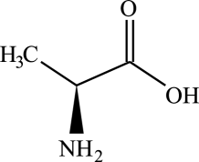
Figure 1: Structure of L-alanine: we label the methyl carbon as qubit 1, the $\alpha$ carbon as qubit 2, and the carboxyl carbon as qubit 3.

With these conventions, we have parameters $J_{12}/2\pi=(34.8\pm 0.2)$ Hz, $J_{23}/2\pi=(53.8\pm 0.2)$ Hz, $\delta_{12}/2\pi=-4.32$ kHz, and $\delta_{13}/2\pi=-20.1$ kHz, where the Larmor frequency of a hydrogen nucleus is $500$ MHz and $J_{13}$ is negligibly small [7, 10]. A $\pi$-pulse with width $\tau\simeq 0.700$ ms, which satisfies $1/\delta_{1k}<\tau\ll\min(1/J_{12},1/J_{23})$, and amplitude $\omega_{1}/2\pi\simeq 714$ Hz, so that $\omega_{1}\tau=\pi$, applied to qubit 1 induces the BS phase shifts $\pi^{2}/(2\delta_{12}\tau)\simeq-0.260$ rad on qubit 2 and $\pi^{2}/(2\delta_{13}\tau)\simeq-0.0559$ rad on qubit 3. Note that this pulse corresponds to a “hard” pulse in the case of a heteronuclear molecule. Considering both pulses involved in the refocusing sequence, we find the total BS phase shifts $\pi^{2}/(\delta_{12}\tau)\simeq-0.519$ rad for qubit 2 and $\pi^{2}/(\delta_{13}\tau)\simeq-0.112$ rad for qubit 3. Clearly, these BS phase shifts are sizable and must be properly taken into account for precise gate operation. The BS effect is usually “compensated” for by book-keeping of the $z$-rotations, so that the phases of the following pulses are adjusted accordingly [11].

3 Cancellation with Soft Pulse

We now propose an alternative implementation of the selective two-qubit operator $U_{23}(\alpha)$. This method has the merit of effectively curbing the BS effect, making it suitable for use with homonuclear molecules. Let us apply to qubit 1 a weak square pulse along the $x$-axis with duration $\tau=\alpha/J_{23}$ and a small amplitude $\omega_{1}$, the value of which will be fixed later so as to eliminate unwanted time evolution.

Let us take the Hamiltonian (1) with constant $\omega_{1}\neq 0$. The time evolution generated by this Hamiltonian for a time $\tau=\alpha/J_{23}$ is

$$e^{-iH(\omega_{1})\tau}=e^{-i(\omega_{1}I_{x}\otimes I_{2}\otimes I_{2}+J_{12}I_{z}\otimes I_{z}\otimes I_{2})\tau}U_{23}(\alpha).$$ (8)

We seek $\omega_{1}$ and $\phi$ such that

$$e^{-i(\omega_{1}I_{x}\otimes I_{2}\otimes I_{2}+J_{12}I_{z}\otimes I_{z}\otimes I_{2})\tau}=e^{i\phi}I_{8}$$ (9)

is satisfied, where $e^{i\phi}$ is an irrelevant global phase. Since the exponent of the left hand side of (9) is traceless, the right hand side must be an element of SU(8) and hence the phase is restricted to the form $\phi=2\pi k/8,k\in\mathbb{Z}$. By explicitly evaluating the left hand side of (9), we find that only 16 out of 64 matrix elements do not vanish in general. These nontrivial equalities are reduced to the following two equations

$$\sin\left(\frac{\alpha}{4}\sqrt{\frac{J_{12}^{2}}{J_{23}^{2}}+\frac{4\omega_{1}^{2}}{J_{23}^{2}}}\right)=0,\ \cos\left(\frac{\alpha}{4}\sqrt{\frac{J_{12}^{2}}{J_{23}^{2}}+\frac{4\omega_{1}^{2}}{J_{23}^{2}}}\right)=\pm 1.$$ (10)

The solutions are $\omega_{1}=\omega_{\pm}$, where

$$\omega_{\pm}=\pm\sqrt{\frac{4\pi^{2}n^{2}J_{23}^{2}}{\alpha^{2}}-\frac{J_{12}^{2}}{4}},\quad n\in\mathbb{N}.$$ (11)

To minimize the BS effect, the magnitude of which is proportional to $\omega_{1}$, $n$ should be the smallest integer such that the radicand of (11) is positive. It turns out that $n=1$ for $J_{ij}$ of L-alanine, which we will consider in the following.

Finally, by applying an rf-field $\omega_{1}=\omega_{\pm}$ for a duration $\tau=\alpha/J_{23}$ we obtain the desired operator $U_{23}(\alpha)$ up to an irrelevant global phase factor. Since $\omega_{1}=\omega_{\pm}$ is considerably smaller than the amplitude of the conventional hard pulses, we expect that the BS effect will be less severe.

Take $\alpha=\pi$, for example, and consider a soft pulse with width $\tau=\pi/J_{23}\simeq 9.29$ ms applied to qubit 1 of a deuterated L-alanine molecule (see section 2). We obtain $\omega_{1}/2\pi\simeq 106$ Hz and find the BS shifts $\omega_{1}^{2}\tau/2\delta_{12}\simeq-0.0762$ rad for qubit 2 and $\omega_{1}^{2}\tau/2\delta_{13}\simeq-0.0164$ rad for qubit 3. Note that we do not need to multiply these phases by 2, since there is only a single pulse applied this time. These results are considerably smaller than those produced by a pair of hard $\pi$-pulses as shown in section 2. In fact, these small phase shifts are comparable to experimental errors and we may simply ignore them in designing quantum gates, which makes pulse programming much easier than with the conventional refocusing pulses.

4 Fidelity

We have shown that, when we want to entangle spins 2 and 3, unwanted time development due to the coupling $J_{12}$ can be eliminated by applying a soft pulse to qubit 1 rather than applying a pair of hard $\pi$-pulses. Note, however, that there have been certain oversimplifications in our analysis: for example, we have ignored the coupling between the rf-field and qubits 2 and 3. We shall now lift some of these assumptions, and employ the full Hamiltonian to evaluate the propagator fidelity for the soft pulse method, and compare it with the fidelity obtained by numerically optimizing the refocusing scheme described in section 2.

Let

$$\hat{H}(\omega_{1}) = \omega_{1}(I_{x}\otimes I_{2}\otimes I_{2}+I_{2}\otimes I_{x}\otimes I_{2}+I_{2}\otimes I_{2}\otimes I_{x})$$ (12)

$$+\delta_{12}I_{2}\otimes I_{z}\otimes I_{2}+\delta_{13}I_{2}\otimes I_{2}\otimes I_{z}$$

$$+J_{12}I_{z}\otimes I_{z}\otimes I_{2}+J_{23}I_{2}\otimes I_{z}\otimes I_{z}$$

be the total Hamiltonian in the common frame rotating with the angular frequency $\omega_{01}$. Here we include the couplings between the rf-pulse with the amplitude $\omega_{1}$ and qubits 1, 2 and 3. For definiteness, let us take $\alpha=\pi$ again and say we would like to implement an entanglement operator

$$U_{23}^{\prime}(\pi)=e^{-i\pi(I_{2}\otimes I_{z}\otimes I_{z})}e^{-i\delta_{12}(\pi/J_{23})(I_{2}\otimes I_{z}\otimes I_{2})}e^{-i\delta_{13}(\pi/J_{23})(I_{2}\otimes I_{2}\otimes I_{z})}$$ (13)

in the common rotating frame. This case ($\alpha=\pi$) is of special interest to us, since it produces the entangling operation for the CNOT gate. Operator (13) reduces to

$$U_{23}(\pi)=\exp(-i\pi I_{2}\otimes I_{z}\otimes I_{z})$$ (14)

in the individual rotating frame, in which each qubit $k$ is described in a frame rotating with the angular velocity $\omega_{0k}$.

Let us denote with $V(\tau,\omega_{1})$ the propagator generated by the refocusing sequence (section 2),

$$V(\tau,\omega_{1})=e^{-i{\hat{H}}(\omega_{1})\tau}e^{-i{\hat{H}}(0)(\pi/(2J_{23})-\tau)}e^{-i{\hat{H}}(\omega_{1})\tau}e^{-i{\hat{H}}(0)(\pi/(2J_{23})-\tau)}$$ (15)

by employing the Hamiltonian (12). Here $\tau$ and $\omega_{1}$ denote the duration and the amplitude of each rf-pulse, respectively, and the whole process is assumed to take a time $\pi/J_{23}$ as before. In a conventional setup, $\omega_{1}$ is taken as $\pi/\tau$. Here, however, we take $\tau$ and $\omega_{1}$ to be independent parameters chosen so that they maximize the propagator fidelity defined below. $V(\tau,\omega_{1})$ consists of four processes: (1) free evolution for a duration $\pi/(2J_{23})-\tau$; (2) evolution under the pulse for a duration $\tau$; (3) free evolution for a duration $\pi/(2J_{23})-\tau$; (4) evolution under the pulse for a duration $\tau$. For vanishingly small values of $\tau$, with $1/|\delta_{1k}|<\tau\ll{\rm min}(1/J_{12},1/J_{23})$, we expect to find the conventional refocusing scheme with hard $\pi$-pulses; then, in an ideal case in which the BS effect were negligible, this propagator would produce the desired entanglement operator.

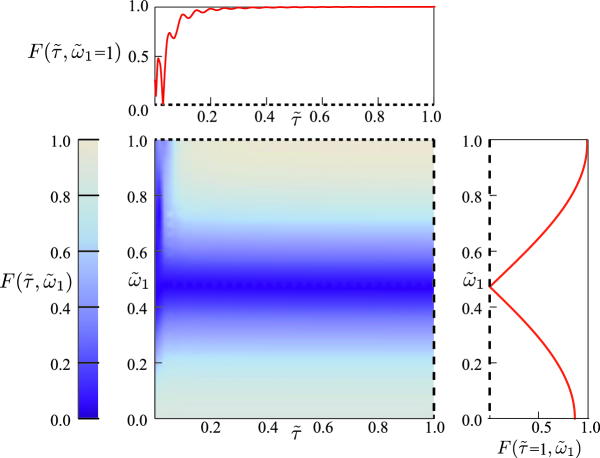
Figure 2: (Color online) Density plot of the propagator fidelity $F(\tilde{\tau},\tilde{\omega}_{1})$ in the domain $0\leq\tilde{\tau}\leq 1$ and $0\leq\tilde{\omega}_{1}\leq 1$ (lower central panel) for the case of deuterated ¹³C-labeled L-alanine. The left panel depicts the scale marks of the function $F\ (0\leq F\leq 1)$ while the right panel shows $F(\tilde{\tau}=1,\tilde{\omega}_{1})$, the fidelity plotted along the dashed line in the lower central panel. The upper panel shows $F(\tilde{\tau},\tilde{\omega}_{1}=1)$, the fidelity plotted along the dotted line in the central panel, corresponding to the conventional refocusing scheme. The global maximum is found for $\tilde{\tau}\simeq 0.947$ and $\tilde{\omega}_{1}\simeq 0.987$, where $F(\tilde{\tau},\tilde{\omega}_{1})\simeq 0.999$.

To compare the unitary matrix resulting from the process (15) with the target operator (13), we define the propagator fidelity

$$F(\tilde{\tau},\tilde{\omega}_{1})=|\mbox{Tr}~{}(U_{23}^{{}^{\prime}\dagger}(\pi)V(\tilde{\tau},\tilde{\omega}_{1}))|/2^{3},$$ (16)

where we have introduced dimensionless parameters $\tilde{\tau}=2J_{23}\tau/\pi$ and $\tilde{\omega}_{1}=\omega_{1}\tau/\pi$. We resort to numerical optimization in order to find the values of $\tilde{\tau}$ and $\tilde{\omega}_{1}$ that maximize the fidelity. Figure 2 shows the fidelity (16) as a function of the normalized pulse width $\tilde{\tau}$ ($0\leq\tilde{\tau}\leq 1$) and the normalized amplitude $\tilde{\omega}_{1}$ ($0\leq\tilde{\omega}_{1}\leq 1$) for the case of deuterated ¹³C-labeled L-alanine (see section 2). We calculate that the global optimal result is given by $F_{\rm opt}\simeq 0.999$ for $\tilde{\tau}\simeq 0.947$ ($\tau\simeq 4.40$ ms) and $\tilde{\omega}_{1}\simeq 0.987$ ($\omega_{1}/2\pi\simeq 112$ Hz).

The conventional refocusing scheme is retrieved by setting $\tilde{\omega}_{1}=1$ (upper central panel in figure 2). In this case, small values of $\tau$ in the interval $1/|\delta_{1k}|<\tau\ll{\rm min}(1/J_{12},1/J_{23})$ correspond to the conventional refocusing scheme with a pair of hard pulses; in particular, for the case of two “hard” $\pi$-pulses with $\tilde{\tau}\simeq 0.151$ ($\tau=0.700$ ms (section 2)), we find $F(0.151,1)\simeq 0.965$. As $\tilde{\tau}$ approaches 1 (so that $\tau$ approaches $\pi/2J_{23}$), the fidelity oscillates slightly about the value $F(1,1)\simeq 0.998$. Let us note that for $\tilde{\omega}_{1}=1$ and $\tilde{\tau}=1$ ($\tau=\pi/2J_{23}\simeq 4.65$ ms, $\omega_{1}/2\pi\simeq 108$ Hz), the two pulses are merged together to form a single $2\pi$-pulse: this choice corresponds to the soft pulse case with a slightly detuned $\omega_{1}$ (see below).

The fidelity for the soft pulse solution obtained in section 3 is easily evaluated by setting $\omega_{1}/2\pi=\omega_{\rm 1sp}/2\pi\simeq 106$ Hz (with $\omega_{\rm 1sp}=\sqrt{4J_{23}^{2}-{J_{12}^{2}}/{4}}$, $\tilde{\omega}_{1}=\tilde{\omega}_{\rm 1sp}\simeq 0.987$) in the Hamiltonian (12) and $\tilde{\tau}=1$, resulting in $F(1,\tilde{\omega}_{\rm 1sp})\simeq 0.999$.

We find that, according to our simulations, the fidelity for the soft pulse scheme (0.999) is better than that obtained with the standard refocusing scheme (0.965) employing hard pulses, and comparable with the fidelity obtained by numerical optimization; moreover, the parameters $\omega_{1}$ and $\tau$ for the soft pulse are conveniently derived from the knowledge of $J_{12}$ and $J_{23}$.

5 Experimental implementation

Let us now provide a concrete example in which we made practical use of the soft pulse technique described above. Consider a system of three qubits, which are all simultaneously afftected by an external noise represented by the fully correlated error channel

$${\mathcal{E}}(\rho) = \sum_{i=0}^{3}p_{i}E_{i}(\rho)E_{i}^{\dagger},$$ (17)

where $E_{0}=\sigma_{0}^{\otimes 3},E_{1}=\sigma_{x}^{\otimes 3},E_{2}=\sigma_{y}^{\otimes 3},E_{3}=\sigma_{z}^{\otimes 3}$. The operators $\{E_{k}\}$ are the Kraus operators (or errors) associated with ${\mathcal{E}}$. Here $p_{i}\geq 0$ is the probability with which an error operator $E_{i}$ acts on the quantum system with density matrix $\rho$, and we assume $\sum_{i=0}^{3}p_{i}=1$. In our recent work [12], we proposed a simple operator quantum error correction scheme which protects one data qubit against this type of noise by encoding it with two ancilla qubits in an arbitrary mixed state. The encoding operator $\mathcal{U}_{E}$ and the decoding operator $\mathcal{U}_{R}$ are implemented with two CNOT gates each. We proved [12] that this scheme provides the simplest noiseless subsystem, in terms of the number of CNOT gates, under our noise model. We implemented this scheme experimentally using a three-qubit NMR quantum computer, in which the ancillae are in the maximally mixed state. We employed a JEOL ECA-500 NMR spectrometer, whose hydrogen Larmor frequency is approximately 500 MHz. As a linear chain molecule with three coupled spins to be used as qubits, we employed ¹³C-labeled L-alanine (98% purity, Cambridge Isotope) solved in D₂O. The quantum circuit takes the form shown in figure 3, wherein we designated the second qubit as the data qubit carrying the information to be protected.

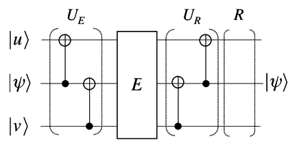
Figure 3: Quantum circuit used in experimental implementation with three-qubit NMR Quantum Computer. The information to be protected is carried by the second qubit.

If we denote the ancillae as $|u\rangle$, $|v\rangle$, and the data qubit as $|\psi\rangle$, it can be shown that,

$$\mbox{Tr}~{}_{1,3}(\mathcal{U}_{R}\circ{\mathcal{E}}\circ\mathcal{U}_{E})(|u\rangle\langle u|\otimes|\psi\rangle\langle\psi|\otimes|v\rangle\langle v|)=|\psi\rangle\langle\psi|,$$ (18)

for any $|u\rangle$, $|v\rangle$, where $\mbox{Tr}~{}_{1,3}$ denotes the partial trace over qubits 1 and 3.

In the experimental pulse sequences realizing the encoding and decoding operations, we employed soft pulses to implement the two two-qubit gates for each operation.

We denote with $U^{\rm sp}_{ij}(\pi)$ the soft pulse operator implementing the two-qubit gate between qubits $i$ and $j$; if we neglect some irrelevant phases, the encoding operation reads (see figure 4)

$$\mathcal{U}^{\rm NMR}_{E}=e^{-i(\pi/2)I_{2}\otimes I_{y}\otimes I_{2}}U^{\rm sp}_{23}(\pi)e^{i(\pi/2)I_{2}\otimes I_{x}\otimes I_{2}}e^{i(\pi/2)I_{y}\otimes I_{2}\otimes I_{2}}U^{\rm sp}_{12}(\pi),$$ (19)

and the deconding operation is

$$\mathcal{U}^{\rm NMR}_{R}=U^{\rm sp}_{12}(\pi)e^{-i(\pi/2)I_{y}\otimes I_{2}\otimes I_{2}}e^{i(\pi/2)I_{2}\otimes I_{x}\otimes I_{2}}U^{\rm sp}_{23}(\pi)e^{i(\pi/2)I_{2}\otimes I_{y}\otimes I_{2}}.$$ (20)

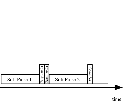
Figure 4: Pulse sequence implementing the encoding operation employing soft pulses. Here $R_{\rm 1{\it y}}(-\pi/2)=e^{i(\pi/2)I_{y}\otimes I_{2}\otimes I_{2}}$, for example.

We find that

$$\begin{array}[]{ccc}\mathcal{U}_{R}E_{0}\mathcal{U}_{E}&=&-4(I_{z}\otimes I_{2}\otimes I_{z}),\\ \mathcal{U}_{R}E_{1}\mathcal{U}_{E}&=&2i(I_{2}\otimes I_{2}\otimes I_{x}),\\ \mathcal{U}_{R}E_{2}\mathcal{U}_{E}&=&-4(I_{y}\otimes I_{2}\otimes I_{x}),\\ \mathcal{U}_{R}E_{3}\mathcal{U}_{E}&=&-4i(I_{x}\otimes I_{2}\otimes I_{z}),\end{array}$$

i.e., upon retrieval, the second qubit is found not to be affected by the noise operators.

Experimental results [12] also show that the algorithm effectively protects the data qubit from the effect of fully correlated noise.

6 Conclusions

We consider a linear chain molecule with three coupled spins and suppose we want to implement an entanglement operator (2) to realize a selective two-qubit gate between spins 2 and 3. In conventional NMR QC, this is achieved by applying a pair of hard $\pi$-pulses to qubit 1. When the molecule is homonuclear, however, one needs to take into account the Bloch-Siegert effect in designing quantum gates. We proposed an alternative method to obtain the entanglement operator (2) by applying a weak pulse to spin 1. Unwanted factors are removed by an appropriate choice of the rf-field amplitude $\omega_{1}$ and duration $\tau$. The BS effect for such a weak pulse is negligible in general, which makes NMR pulse programming and quantum gates design much simpler than with conventional hard $\pi$-pulses; it also makes this method suitable for use with both homo- and heteronuclear molecules. We employed the proposed scheme in an operator quantum error correction experiment [12]. This technique should be also applicable to any physical system, for which the coupling constants are not controllable.

References

References

- [1] Nakahara M and Ohmi T 2008 Quantum Computing: From Linear Algebra to Physical Realizations (London: Taylor & Francis)
- [2] Nielsen M A and Chuang I L 2000 Quantum Computation and Quantum Information (Cambridge: Cambridge University Press)
- [3] Vandersypen L M K 2001 Quantum Experimental Quantum Computation with Nuclear Spins in Liquid Solution (Stanford University Thesis)
- [4] Bloch F and Siegert A 1940 Phys. Rev. 57 522
- [5] Ramsey N F 1940 Phys. Rev. 100 1191
- [6] Emsley L and Bodenhausen G 1990 Chem. Phys. Lett. 168 297
- [7] Kondo Y 2009 Molecular Realizations of Quantum Computing 2007 (Kinki University Series on Quantum Computing vol.2) ed M Nakahara, Y Ota et al. (Singapore: World Scientific Publishing) p 1
- [8] Kondo Y, Nakahara M and Tanimura S 2006 Physical Realizations of Quantum Computing, ed M Nakahara, S Kanemitsu et al. (Singapore: World Scientific Publishing) p 127
- [9] Jones J A 2001 Prog. NMR Spectrosc. 38 325–360
- [10] Kondo Y 2007 J. Phys. Soc. Japan 76 104004
- [11] See, for example, Cory D G, Laflamme R et al. Preprint arXiv:quant-ph/0004104v1
- [12] Kondo Y, Bagnasco C and Nakahara M 2013 Phys. Rev. A 88 022314