Validating Network Value of Influencers by means of Explanations

Abstract

Recently, there has been significant interest in social influence analysis. One of the central problems in this area is the problem of identifying influencers, such that by convincing these users to perform a certain action (like buying a new product), a large number of other users get influenced to follow the action. The client of such an application is essentially a marketer who would target these influencers for marketing a given new product, say by providing free samples or discounts. It is natural that before committing resources for targeting an influencer the marketer would be interested in validating the influence (or network value) of influencers returned. This requires digging deeper into such analytical questions as: who are their followers, on what actions (or products) they are influential, etc. However, the current approaches to identifying influencers largely work as a black box in this respect. The goal of this paper is to open up the black box, address these questions and provide informative and crisp explanations for validating the network value of influencers.

We formulate the problem of providing explanations (called Proxi) as a discrete optimization problem of feature selection. We show that Proxi is not only NP-hard to solve exactly, it is NP-hard to approximate within any reasonable factor. Nevertheless, we show interesting properties of the objective function and develop an intuitive greedy heuristic. We perform detailed experimental analysis on two real world datasets – Twitter and Flixster, and show that our approach is useful in generating concise and insightful explanations of the influence distribution of users and that our greedy algorithm is effective and efficient with respect to several baselines.

I Introduction

The study of social influence has gained tremendous attention in the field of data mining ever since the seminal paper of Kempe et al. [14] on the problem of influence maximization. A primary motivating application for influence maximization as well as for other closely related problems such as identifying community leaders [9], trendsetters [21], influential bloggers [1] and microbloggers [24, 5], is viral marketing. The objective in these problems is to identify influential users (also called influencers or seeds) in a social network such that by convincing these users to perform a certain action (like buying a new product), a large number of other users can be influenced to follow the action. The client of such an application is essentially a marketer who would target these influencers for marketing a given new product, e.g., by providing free samples or discounts. It is natural that the marketer would like to analyze the influence spread [14] or “network value” [6] of these influencers before actually committing resources for targeting them. She would be interested in the answers to the following questions: Where exactly does the influence of an influencer lie? How is it distributed? On what type of actions (or products) is an influencer influential? What are the demographics of its followers? However, the current approaches for identifying influencers, and in particular, for selecting seed users for the problem of influence maximization, largely work as a black box in this respect. Just outputting a list of seed users (influencers), along with a scalar which is an estimate of the expected influence spread. The goal of this paper is to open up this black box, address these questions and provide informative and crisp explanations for the influence distribution of influencers.

Providing explanations to the marketer for influence spread of influencers can have several benefits. First, it provides transparency to the seed selection algorithm. The marketer is made aware of why a certain user is selected as a seed, where the user’s influence lies, and on what type of actions the user is influential. These are important analytics she may want to investigate before spending resources on targeting that seed user. Second, it makes the seed selection algorithm (and thus the system) scrutable. The marketer would now be able to tell the system, if the explanations (and thus the algorithm) are wrong or are based on incorrect assumptions, say using her own surveys or background knowledge. If the explanations are correct and accurate, this can increase the marketer’s trust in the system and help her in making good, informed decisions quicker. In other words, accurate explanations may enhance effectiveness and efficiency of the marketers, in making important marketing decisions. Furthermore, such explanations allow room for flexibility in the targeting process. Indeed, if the marketer is not able to target some of the seeds successfully, then she knows what exactly the impact on “coverage” would be, and can make adequate adjustments. For example, if a seed’s influence was over young college students in CA on handheld devices, the marketer can look for an alternate seed with close characteristics to cover that demographic. Overall, providing accurate and crisp explanations would increase the marketer’s satisfaction, and hence loyalty to the provider of seed selection service, as well as confidence in the seed selection algorithm. In this paper, we specifically focus on providing explanations for influencer validation, that is, a marketer would be able to analyze the demographics of the followers and the actions.

On the industry side, companies like Klout and Peerindex claim to provide users’ influence scores from their Social Media profiles (like Facebook and Twitter). Both these companies provide “topics” over which the users’ influence is spread, in addition to influence scores. The explanations we propose offer a principled and comprehensive account of just how the influence of a seed user is distributed across the user (i.e., follower) and action dimensions instead of an ad hoc “influence score” and “topic”.

The merit of providing explanations has been recognized before, in the related fields of recommender systems (see Chapter 15 of [19] for a survey) and expert systems (see [15] for a review). In these systems, the explanations are known to have benefits similar to those mentioned above. In the field of social influence analysis, to the best of our knowledge, there has been no such systematic study.

TABLE I: Mike: User with most followups. $k=6$, $l=3$.

			Actions	Followers	Followups
			(3.0k)	(106)	(37.9k)
rated R	thriller	male	708	67	6.7k
		female	708	37	2.3k
male	drama	len:long	480	67	4.8k
		len:med	520	67	3.5k
pre-1997	comedy	male	607	67	4.8k
		female	607	37	2.2k
Total Coverage:					56.3%

A Motivating Example. Consider a social network where users perform actions. For instance, in Flixster (www.flixster.com), user actions correspond to rating movies. A movie can have many attributes, e.g., genre, year of release, length of the movie, rating value, and similarly, users can have many attributes, e.g., gender, age-group and occupation. Table I shows an example of the result from our experimental analysis on the real data of Flixster. In this example, we analyze the influence of the top influencer in Flixster, measured in terms of number of followups. For simplicity, we refer to this user as Mike. Informally, a followup is defined as a follower following up on a user’s action. In the context of this example, the number of followups of Mike is the number of times a follower of Mike rated a movie, after he rated it.

The table makes the following assertions. Mike has rated 3K movies and has 106 active followers. In total, he has received 37.9K followups. This is the overall picture of Mike’s influence spread. Drilling down, the table shows six explanations describing a partial breakdown that covers a significant chunk of the influence mass, each explanation corresponding to a row. Each explanation is presented in terms of action and user features (first three columns). The explanations are heterogeneous: e.g., the first two explanations involve attributes maturity rating, genre, and user gender, whereas the next two involve the attributes user gender, genre, and movie length.

With just 6 crisp explanations, our algorithm is able to explain 56.3% of Mike’s followups. As an example, 6.7K followups came from male followers, on Mike’s ratings on thriller movies rated R. (movies restricted to persons of age 17 or older). Moreover, 2.3K followups came from females on the same category of movies, suggesting that Mike is quite influential on R-rated thriller movies. The Actions column tells us that there are 708 such movies (thriller, rated R) that are rated by Mike, while the Followers column tells us that out of 106 followers, 67 are males and 37 are females and 2 (= 106 - (67 + 37)) others did not specify their gender. Other explanations reveal that Mike is also influential on drama movies on males, and old (pre-1997) comedy movies regardless of gender.

Notice, the entries in each of the numeric columns (Action/Followers Count and Followups) do not sum to their overall values. That is, in general, the explanations provided do not necessarily completely cover the entire influence spread of the seed user. Each explanation consists of a description involving follower (user) demographics and action attributes (e.g., topic). It also comes equipped with three statistics – action count, follower count, and followups, with the meaning described above. It is possible that different explanations cover overlapping demographics, e.g., females in Vancouver and young college students in BC.

There are several benefits to this style of explanations in terms of affording simple inferences. First, we can deduce that if Mike (in the example above) rates an arbitrary movie again, he is likely to receive 37.9K/3K = 12.6 followups on average. Next, we know on what kinds of movies Mike is influential. Thus, if a marketer wants to advertise a horror movie, then perhaps Mike is not a good seed, even though his influence is quite high. Moreover, if Mike rates a thriller movie rated R, it is likely that it will attract 6.7K/708 = 9.5 followups, from male users on average. Clearly, these types of explanations are very informative and valuable.

Notice that a trivial answer to providing explanations is to describe every single followup for a given influencer. This is undesirable since such an explanation would be verbose and uninformative to the marketer trying to make sense of the influencer’s influence. We thus argue for providing crisp or concise explanations that explain as much of the influence spread (in terms of followups) of the influencer, as possible.

In the literature, the network value of a user [6, 14] is treated as a scalar, i.e., it’s equated with the (expected) influence spread of the user. We argue that in order to answer the above questions, we must revisit this notion. Our thesis is that there is much more to the network value of a user than just a number: it can be seen as a summary of the influence distribution of the user, which describes how the influence is distributed, over what kind of user demographics and on what type of actions. In this paper, we formulate and attack the problem of how to characterize the distribution of influence of a given seed user. In particular, we make the following contributions.

• We propose a novel problem of PROviding eXplanations for Influencers’ validation (Proxi) to describe network value of a given influencer. We outline several benefits of providing explanations.

• We show that Proxi is not only NP-hard to solve exactly, it is NP-hard to approximate within any reasonable factor. However, by exploiting properties of the objective function, we develop an intuitive greedy heuristic.

• We perform experimental analysis on two real datasets – Flixster and Twitter, by exploring the influence distributions of top influencers, from both qualitative and quantitative angles.

• Performing qualitative analysis, we establish the validity of our framework, while gaining insights into influence spread of influencers. On the other hand, with quantitative analysis, we show that our algorithm explains a significant amount of the influence spread with a small number of crisp explanations. We compare our algorithm with various baselines, and show that it is both effective and efficient.

The rest of the paper is organized as follows. Related work is discussed in §II. We formalize the problem in §III and develop our algorithm in §IV. The experimental analysis is presented in §V, while §VI summarizes the paper and discusses future work.

II Related Work

We summarize related work under three headings.
Identifying Influencers. Identifying influencers has been extensively studied as the problem of influence maximization. The first work of this kind is due to Domingos et al. [6]. They refer to users’ influence as network value and model it as the expected lift in profit due to influence propagation. Thus, the network value of a customer is captured as a number. Later, Kempe et al. [14] formulated this as a discrete optimization problem: select $k$ influencers in a given social network such that by targeting them, the expected spread of the influence is maximized, assuming the propagation follows a diffusion model such as independent cascades or linear threshold or their variants. The problem is NP-hard. However, the objective function satisfies the nice properties of monotonicity and submodularity, under the diffusion models considered, allowing a simple greedy algorithm to provide a $(1-1/e-\epsilon)$-approximation to the optimal solution, for any $\epsilon>0$ [18]. Further exploiting these properties, Leskovec et al. [16] proposed a lazy forward optimization that dramatically improves the efficiency of the greedy algorithm. The idea is that the marginal gain of a node in the current iteration cannot be better than its marginal gain in the previous iterations. Goyal et al. [10] proposed a direct data driven approach to social influence maximization. They show this alternative approach is both accurate (in predicting the influence spread) and is scalable, compared to the probabilistic approach of Kempe et al. [14]. Their work also highlights the importance of validating the influence prediction and spread.

Considerable work has been done on analyzing social influence on blogs and micro-blogs. Agarwal et al. [1] investigate the problem of identifying influential bloggers in a community. They show the most influential bloggers are not necessarily the most active. Gruhl et al. [11] analyze information diffusion in blogspace by characterizing the individuals and the topics of their blog postings. In [8], the authors look into the problem of inferring networks of diffusion and influence in blogspace. Weng et al. [24] develop a topic sensitive Pagerank-like measure (called Twitterrank) for ranking users based on their influence on given topics. Cha et al. [5] compare three different measures of influence – indegree (number of followers), retweets and user mentions, with regard to their ability to characterize influencers. They observe that users who have a large number of followers are not necessarily influential in terms of spawning off retweets or mentions. Romero et al. [20] showed that the majority of users act as passive information consumers and do not forward the content to the network. Bakshy et al. [2] find that the largest cascades tend to be generated by users who have been influential in the past and who have a large number of followers.

The problem of identifying influencers, and indeed influence maximization, is fundamentally different from our problem Proxi. The objective of Proxi is to allow a human (or marketer) to (independently) validate a given influencer, by generating human readable, crisp explanations. The explanations consist of features from action and user dimensions with relevant statistics and are generated in a way such that they are able to cover the maximum amout influence, in terms of followups.

Since our explanations are built of action and user features, works on topic-sensitive influence analysis [23, 17, 24, 21, 3] and influence based community detection [9, 4] are relevant and we survey these next.

Topics. Tang et al. [23] introduce the problem of topic-based social influence analysis. Given a social network and a topic distribution for each user, the problem is to find topic-specific subnetworks, and topic-specific influence weights between members of the subnetworks. Liu et al. [17] propose a generative model which utilizes the content and link information associated with each node (which can be a user, or a document) in the network, to mine topic-level direct influence. They use Gibbs sampling to estimate the topic distribution and influence weights. Weng et al. [24], as described earlier, propose a topic sensitive Pagerank-like measure to rank users of Twitter. In [21], the authors define trendsetters as the “early adopters” who spread the new ideas or trends before they become popular. They also propose a Pagerank-like measure to identify trendsetters. Barbieri et al. [3] extend classical propagation models like linear threshold and independent cascade [14] to handle topic-awareness. Our problem is given a network, past information cascades in the form of an action log, and a seed node, we need to generate a compact explanation of the way the influence spread of the seed is distributed, which is not addressed by any of these works.

Communities. Another related line of work is influence-based community detection [9, 4]. Goyal et al. [9] define the notion of “tribe-leaders” – leaders (or influencers) who are followed up by the same set of users, on several actions. They apply a pattern mining framework to discover them. Barbieri et al. [4] propose a generative model to detect communities incorporating information cascades.

In contrast to the above mentioned papers, our goal is not to model topics or to detect communities, but to describe the influence distribution of a given user, by generating explanations consisting of interesting features from action and user dimensions. To the best of our knowledge, this is the first research study to provide explanations for the purpose of influencer validation.

III Problem Definition

We consider a directed social graph, $G=(V,D)$ over a set of users $V$ where each arc $(u,v)\in D$ indicates that user $v$ follows user $u$, and a propagation log $\mathbb{L}$, a set of triples $(u,a,t_{u})$ signifying that user $u$ performed action $a$ at time $t_{u}$. When the action $a$ is clear from the context, by $t_{u}$ we mean the time at which user $u$ performed action $a$. We say an action $a$ is propagated from $u$ to $v$ if $(u,v)\in D$, and the log $\mathbb{L}$ cotains the tuples $(u,a,t_{u})$ and $(v,a,t_{v})$ for some $t_{u}$ and $t_{v}$, such that $t_{u}<t_{v}$. This defines a propagation graph of $a$ as a directed graph $G(a)=(V(a),D(a))$, with $V(a)=\{u\in V|\exists t_{u}:(u,a,t_{u})\in\mathbb{L}\}$ and $D(a)=\{(u,v)\in D|u\in V(a),v\in V(a),\mbox{ and }t_{u}<t_{v}\}$. Define an influence cube $\mathcal{C}$ over the dimensions Users (as influencers), Actions and Users (as followers) as follows: for a cell $(u,a,v)$, $\mathcal{C}(u,a,v)=1$ if there exists a (directed) path from $u$ to $v$ in $G(a)$, i.e., $v$ performed action $a$ after $u$ did. All other cells have value $0$.

Given a user $u$, by a followup of u, we mean a cell $(u,a,v)$ for which $\mathcal{C}(u,a,v)=1$. The followup set of $u$ is then the set of followups of $u$: $\mathcal{M}_{u}=\{(u,a,v)\mid\mathcal{C}(u,a,v)=1\}$. When the user is understood from the context, we use $\mathcal{M}$ instead of $\mathcal{M}_{u}$. We assume users are equipped with a set of features (e.g., age, location etc), and similarly for actions (e.g., topic). Descriptions for followup sets are derived from attributes by means of predicates of the form $\texttt{A}=\texttt{val}$ where A is an attribute and val is a value from its domain. We assume numeric attributes are binned into appropriate intervals. Thus it suffices to consider only equality. E.g., year = pre-1997, maturity-rating = “rated R”, and gender = female are predicates/features. We use the terms predicates and features interchangeably. Let $\mathcal{P}$ be the set of all predicates. Consider a cell $(u,a,v)$ in $\mathcal{M}_{u}$, the followup set of user $u$, and a predicate $p\in\mathcal{P}$, we say the cell satisfies the predicate, $(u,a,v)\models p$, provided either $p$ is a user predicate and user $u$ satisfies this predicate or $p$ is an action predicate and action $a$ satisfies this predicate. For a predicate $p$, we define $\mathcal{M}^{p}=\{(u,a,v)\mid(u,a,v)\in\mathcal{M}\,\&\,(u,a,v)\models p\}$, i.e., the subset of followups satisfying the predicate. We define an explanation as a conjunction of one or more (user and/or action) predicates. Given an explanation $E$, we define $\mathcal{M}^{E}=\bigcap_{p\in E}\mathcal{M}^{p}$. i.e., the set of followups satisfying all the predicates in $E$. We define the coverage of an explanation to be $\sigma(E)=|\mathcal{M}^{E}|$, i.e., the number of followups satisfying $E$.

Our goal is to provide explanations for the followup set of a user (candidate influencer). On one hand, we would like each explanation to be as informative as possible. On the other, the total size of explanations should be concise or crisp so that a human (marketer) can quickly make sense of them. At the same time, between them, the explanations should cover as much “influence mass” as possible. We formalize these intuitions by insisting that each explanation should have length $\geq l$ and ask for a set of at most $k$ explanations $\mathcal{E}=\{E_{1},...,E_{k}\}$ such that the number of followups covered by these explanations is as large as possible. For a set of explanations $\mathcal{E}$, we extend coverage as follows: define $\mathcal{M}^{\mathcal{E}}=\bigcup_{E\in\mathcal{E}}\mathcal{M}^{E}$ and finally, define the coverage of a set of explanations as $\sigma(\mathcal{E})=|\mathcal{M}^{\mathcal{E}}|$, i.e., the number of followps in $\mathcal{M}$ which satisfy at least one explanation in $\mathcal{E}$. That is,

$$\sigma(\mathcal{E})=|\mathcal{M}^{\mathcal{E}}|=|\bigcup_{E\in\mathcal{E}}\mathcal{M}^{E}|=|\bigcup_{E\in\mathcal{E}}\bigcap_{p\in E}\mathcal{M}^{p}|$$ (1)

Note the term coverage is defined for a single explanation as well as for a set of explanations. In discussing the properties of the coverage function, we consider both $\sigma(E):2^{\mathcal{P}}\rightarrow\mathbb{R}$, coverage of a single explanation as a function of the features in the explanation, as well as $\sigma(\mathcal{E}):2^{2^{\mathcal{P}}}\rightarrow\mathbb{R}$, coverage of a set of explanations as a function of the explanations in the set $\mathcal{E}$. The notation and the context should make it clear.

The main problem we study in this paper is Proxi (PROviding eXplanations for validating the network value of Influencers):

Problem 1 (Proxi)

Given a user $u$, followup set $\mathcal{M}$, the available user and action predicates $\mathcal{P}$, and numbers $k$ and $l$, find a set of at most $k$ explanations $\mathcal{E}=\{E_{1},...,E_{k}\}$, where each explanation $E_{i}$ is a conjunction of at least $l$ (user/action) predicates such that $\sigma(\mathcal{E})$ is maximized.

The lower bound $l$ on the size of each explanation captures the intuition that explanations should be informative. The upper bound $k$ on the number of explanations captures the intuition that overall the explanations should be crisp. At the same time, problem asks for the influence mass covered (coverage) to be maximum.

III-A Hardness of PROXI

Not surprisingly, it turns out that Proxi is NP-hard. Unfortunately though, not only it is NP-hard to solve exactly, it is NP-hard to approximate within any reasonable factor, even when $k=1$, which in other words is the problem of generating one explanation (Thm. 1). We establish the hardness by exploiting its equivalence with the problem of Maximum $l$-Subset Intersection (MSI for short). However, to develop intuitions for building our algorithm, we show some interesting properties of the objective function $\sigma(\mathcal{E})$. In particular, we show that the function $\sigma(\mathcal{E})$ is monotonically increasing and submodular (Thm. 2), while the function $\sigma(E)$ is monotonically decreasing and supermodular (Thm. 3). We exploit these results to develop our algorithm (§IV).

Theorem 1

Problem Proxi is NP-hard to solve exactly. Moreover, it cannot be approximated within a factor of $0.5n^{1-2\epsilon}+O(1-3\epsilon)$ for any $\epsilon>0$, unless P=NP.

Proof:

We prove the claim for the special case when $k=1$. In this case, the problem reduces to finding exactly one explanation $E$, of length $l$ such that $\sigma(E)$ is maximized. Since $\sigma(E)$ is defined as the intersection of sets $\mathcal{M}^{p}$ for all $p\in E$, the problem is equivalent to Maximum $l$-Subset Intersection (MSI) Problem [25, 22]: Given a collection of sets $\mathcal{S}=\{S_{1},S_{2},\ldots,S_{m}\}$ over a universe of elements $\mathcal{U}=\{e_{1},e_{2},\ldots,e_{n}\}$, the objective is to select (no less than) $l$ sets $\mathcal{S}^{\prime}\subseteq\mathcal{S}$, $\mathcal{S}^{\prime}=\{S_{i_{1}},S_{i_{2}},\ldots,S_{i_{l}}\}$ such that its intersection size, $|S_{i_{1}}\cap S_{i_{2}}\cap\cdots S_{i_{l}}|$, is maximum.

It is easy to see that MSI is equivalent to Proxi when $k=1$. An element $e\in\mathcal{U}$ in MSI corresponds to a cell $(u,a,v)$ with a value 1 in Proxi. Similarly, a set $S$ corresponds to $\mathcal{M}^{p}$, the set of cells selected by a predicate $p$. Furthermore, the objective is equivalent – select $l$ sets ($l$ predicates) such that the resulting intersection size is maximum. The formal reduction from MSI to Proxi and the other way around is thus straightforward and we skip it for brevity.

It is well known that MSI is NP-hard, and is NP-hard to approximate it within a factor a $0.5n^{1-2\epsilon}+O(1-3\epsilon)$ [22]. Given the equivalence between Proxi and MSI, the theorem follows. ∎

Theorem 2

The function $\sigma(\mathcal{E}):2^{2^{\mathcal{P}}}\rightarrow\mathbb{R}$ is monotonically increasing and submodular. That is, $\forall\mathcal{E}\subseteq\mathcal{E}^{\prime}\subseteq 2^{2^{\mathcal{P}}}:\sigma(\mathcal{E})\leq\sigma(\mathcal{E}^{\prime})$ and $\sigma(\mathcal{E}\cup\{E\})-\sigma(\mathcal{E})\geq\sigma(\mathcal{E}^{\prime}\cup\{E\})-\sigma(\mathcal{E}^{\prime})$.

Proof:

First, we show that the objective function $\sigma(\mathcal{E})$ is monotonically increasing. By definition of $\sigma(\mathcal{E})$, we have,

$$\sigma(\mathcal{E}\cup\{E\})-\sigma(\mathcal{E})=|\mathcal{M}^{\mathcal{E}}\cup\mathcal{M}^{E}|-|\mathcal{M}^{\mathcal{E}}|$$

Clearly, $\mathcal{M}^{\mathcal{E}}\cup\mathcal{M}^{E}$ is a superset of $\mathcal{M}^{\mathcal{E}}$, the above quantity is non-negative, implying that $\sigma(\mathcal{E})$ is monotonically increasing. Next, we show the property of submodularity.

$$\sigma(\mathcal{E}^{\prime}\cup\{E\}) -\sigma(\mathcal{E}^{\prime})=|\mathcal{M}^{\mathcal{E}^{\prime}}\cup\mathcal{M}^{E}|-|\mathcal{M}^{\mathcal{E}^{\prime}}|$$

$$=|(\mathcal{M}^{\mathcal{E}^{\prime}}\cup\mathcal{M}^{E})\setminus\mathcal{M}^{\mathcal{E}^{\prime}}|$$

$$=|(\mathcal{M}^{\mathcal{E}}\cup\mathcal{M}^{\mathcal{E}^{\prime}}\cup\mathcal{M}^{E})\setminus(\mathcal{M}^{\mathcal{E}}\cup\mathcal{M}^{\mathcal{E}^{\prime}})|$$

$$=|((\mathcal{M}^{\mathcal{E}}\cup\mathcal{M}^{E})\setminus\mathcal{M}^{\mathcal{E}})\setminus\mathcal{M}^{\mathcal{E}^{\prime}}|$$

Since set subraction may only remove set elements,

$$\sigma(\mathcal{E}^{\prime}\cup\{E\})-\sigma(\mathcal{E}^{\prime}) \leq|(\mathcal{M}^{\mathcal{E}}\cup\mathcal{M}^{E})\setminus\mathcal{M}^{\mathcal{E}}|$$

$$\leq\sigma(\mathcal{E}\cup\{E\})-\sigma(\mathcal{E})$$

which is what we wanted to prove. ∎

Theorem 3

The function $\sigma(E):2^{\mathcal{P}}\rightarrow\mathbb{R}$ is monotonically decreasing and supermodular. That is, $\forall E\subseteq E^{\prime}\subseteq 2^{\mathcal{P}}:\sigma(E)\geq\sigma(E^{\prime})$ and $\sigma(E\cup\{p\})-\sigma(E)\leq\sigma(E^{\prime}\cup\{p\})-\sigma(E^{\prime})$.

Proof:

First, we show that the objective function $\sigma(E)$ is monotonically decreasing. By definition of $\sigma(E)$, we have,

$$\sigma(E\cup\{p\})-\sigma(E)=|\mathcal{M}^{E}\cap\mathcal{M}^{p}|-|\mathcal{M}^{E}|$$

Clearly, $\mathcal{M}^{E}\cap\mathcal{M}^{p}$ is a subset of $\mathcal{M}^{E}$, the above quantity is non-positive, implying that $\sigma(E)$ is monotonically decreasing. We next show the property of supermodularity.

$$\sigma(E^{\prime}\cup\{p\}) -\sigma(E^{\prime})=-(|\mathcal{M}^{E^{\prime}}|-|\mathcal{M}^{E^{\prime}}\cap\mathcal{M}^{p}|)$$

$$=-|\mathcal{M}^{E^{\prime}}\setminus(\mathcal{M}^{E^{\prime}}\cap\mathcal{M}^{p})|$$

$$=-|(\mathcal{M}^{E}\cap\mathcal{M}^{E^{\prime}})\setminus(\mathcal{M}^{E}\cap\mathcal{M}^{E^{\prime}}\cap\mathcal{M}^{p})|$$

$$=-|\mathcal{M}^{E^{\prime}}\cap(\mathcal{M}^{E}\setminus(\mathcal{M}^{E}\cap\mathcal{M}^{p}))|$$

Since set intersect may only remove set elements,

$$\sigma(E^{\prime}\cup\{p\})-\sigma(E^{\prime}) \geq-|(\mathcal{M}^{E}\setminus(\mathcal{M}^{E}\cap\mathcal{M}^{p})|$$

$$\geq\sigma(E\cup\{p\})-\sigma(E)$$

which is what we wanted to prove. ∎

IV Algorithm

Even though Proxi is NP-hard to approximate, the function $\sigma(\mathcal{E})$ has nice properties as we show in Theorem 2. Nemhauser et al. [18] show that maximizing monotonically increasing submodular functions can be approximated within a factor of $(1-1/e)$ using a greedy algorithm. Moreover, due to Feige [7], we know that this is the best possible approximation factor that can be achieved in polynomial time. These results, in addition to Theorem 2, suggest that the greedy heuristic which adds the current best explanation $E$ to $\mathcal{E}$, until $|\mathcal{E}|$ is $k$ would be the best possible heuristic. However, the complex step here is to generate one explanation $E$, or more generally, the next explanation $E$, such that the marginal coverage $\sigma(\mathcal{E}\cup\{E\})-\sigma(E)$ maximized, where $\mathcal{E}$ is the current set of explanations. We showed that this particular problem is NP-hard to approximate (see the proof of Theorem 1). Thus, strictly speaking, we cannot expect to have an efficient algorithm with a provable approximation guarantee for Proxi.

However, given the hardness of the problem, we believe that a greedy algorithm of successively generating explanations by repeatedly picking the best predicate would still be a good heuristic. More precisely, in any iteration, where $\mathcal{E}:|\mathcal{E}|<k$ is the current set of explanations and $E:|E|<l$ is the current explanation, the greedy algorithm picks the predicate, $p$, that when added to $E$ gives an extended explanation that provides the maximum possible additional coverage, w.r.t. $\mathcal{E}$. That is, $\sigma(\mathcal{E}\cup\{E\cup\{p\}\})-\sigma(\mathcal{E})$ is maximum.

Since the search space is massive, a naive greedy algorithm as explained above would be extremely slow. So we focus our attention on making the algorithm efficient, by cleverly avoiding unnecessary coverage evaluations, in any given iteration. In particular, we optimize our algorithm by means of lazy evaluation. Recall, the function $\sigma(E):2^{{\cal P}}\rightarrow\mathbb{R}$ is non-increasing and supermodular. Thus, the lazy forward approach used by Leskovec et al. [16] does not work here, as it relies on the non-decreasing submodular nature of the objective function. We instead exploit the fact that the coverage of a single explanation $\sigma(E):2^{{\cal P}}\rightarrow\mathbb{R}$ is non-increasing in the number of features (predicates), and devise a lazy evaluation optimization based on this. The idea is that, while constructing a single explanation, the marginal coverage of the explanation after adding a predicate $p$ to explanation $E$ also cannot increase (since $\sigma(E)$ is non-increasing). Thus, by maintaining a max-heap of predicates, $p$, sorted on additional coverage of the extended explanation $E\cup\{p\}$ w.r.t. $\mathcal{E}$, we can avoid coverage recomputations for many of the predicates, in any given iteration.

We next explain our algorithm in detail, given in Algorithms 1 and 2. In $Q$, we store the max-heap of features. Each element $p$ in $Q$ represents a predicate/feature with the following attributes: $p.cells$ denotes the set of cells corresponding to the predicate, or equivalently $\mathcal{M}^{p}$; $p.cov$ denotes the effective additional coverage of an explanation, $E$, w.r.t. $\mathcal{E}$, if $p$ were added to the explanation, that is, $p.cov=\sigma(\mathcal{E}\cup\{E\cup\{p\}\})-\sigma(\mathcal{E})$. Due to our lazy evaluation optimization, $p.cov$ may not always store the correct value. Instead, it may store an outdated value, which may have been calculated in some earlier iteration. To keep track of it, we use $p.flag$ to save the iteration when $p.cov$ was last updated. Moreover, we mark a cell when it is covered by the current set of explanations. Initially, all cells are unmarked, and $p.flag$ for all the features is set to $0$. The heap $Q$ is sorted on $p.cov$. Our main subroutine MineExplanations adds one explanation $E$ at a time, in a greedy fashion, while the subroutine NextExplanation generates the next best explanation, again in a greedy fashion.

Algorithm 1 MineExplanations

0:  $Q$, $k$, $l$

0:  $\mathcal{E}$

1:  $\mathcal{E}\leftarrow\emptyset$.

2:  while $|\mathcal{E}|<k$ do

3:     $p\leftarrow Q.peek()$.

4:     if $p.flag<|\mathcal{E}|\cdot l$ then

5:       $Q.poll()$.

6:       $p.cov\leftarrow$ #cells in $p.cells$ for which $cell$ is not marked.

7:       $p.flag\leftarrow|\mathcal{E}|\cdot l$.

8:       Reinsert $p$ in $Q$ (and reheapify w.r.t. $p.cov$).

9:     else

10:       $Q^{\prime}\leftarrow copy(Q)$ (copy includes features’ coverage).

11:       $E\leftarrow\textsc{NextExplanation}(Q^{\prime},l,|\mathcal{E}|)$.

12:       $\mathcal{E}\leftarrow\mathcal{E}\cup\{E\}$.

Algorithm 2 NextExplanation

0:  $Q^{\prime}$, $l$, $|\mathcal{E}|$

0:  $E$

1:  $E\leftarrow\emptyset$.

2:  while $|E|<l$ do

3:     $p\leftarrow Q^{\prime}.poll()$.

4:     if $p.flag<|\mathcal{E}|\cdot l+|E|$ then

5:       $p.cov\leftarrow$ #cells in $p.cells$ for which $cell.flag=|\mathcal{E}|\cdot l+|E|$ and $cell$ is not marked.

6:       $p.flag\leftarrow|\mathcal{E}|\cdot l+|E|$.

7:       Reinsert $p$ in $Q^{\prime}$ (and reheapify w.r.t. $p.cov$).

8:     else

9:       $E\leftarrow E\cup\{p\}$.

10:       for each $cell\in p.cells$ do

11:          if $|E|=l$ and $cell.flag=|\mathcal{E}|\cdot l+l$ then

12:              mark the cell.

13:          else if $|E|=1$ then $cell.flag\leftarrow|\mathcal{E}|\cdot l+1$.

14:          else $cell.flag\leftarrow cell.flag+1$.

We first describe Algorithm MineExplanations. $\mathcal{E}$ is initialized in line 1 and we iterate until $k$ explanations are generated (lines 2-12). In each of these $k$ iterations, we get the next best explanation by calling NextExplanation, and add it to $\mathcal{E}$ (lines 10-12). We make a copy of $Q$ before calling NextExplanation, because the ordering of the heap $Q$ can be changed by the subroutine, and thus corrupt the original ordering. Other lines of the algorithm implement the lazy evaluation optimization. The feature with the maximum coverage is taken from the heap $Q$, without removing the it from $Q$ (i.e., $peek()$, in line 3). If there is a need to recompute the coverage $p.cov$ of the feature $p$ (this condition is tested using $p.flag$), then we do so in line 6, after removing it from $Q$ in line 5 (i.e., $poll()$). The flag is updated in line 7 and the heap $Q$ is re-heapified accordingly.

Next, we describe Algorithm 2, which generates one explanation at a time. This algorithm also employs a greedy strategy to select the features in a lazy manner. $E$ is initialized in line 1 and we iterate until we generate $l$ features in $E$. In this subroutine, we also assign a $flag$ to each cell. Intuitively, $cell.flag$ stores the number of features in the current explanation $E$ that covers the cell. For example, $cell.flag$ is $|\mathcal{E}|\cdot l+1$, if it is covered by exactly one feature in $E$, and similarly, it is $|\mathcal{E}|\cdot l+|E|$ when all features in $E$ cover the cell. It should be noted that the term $|\mathcal{E}|\cdot l$ is added to ensure that the flag values across different iterations of Algorithm 1 don’t mix up.

We again exploit $p.flag$ to track the iteration when the coverage of the predicate/feature was last updated. As in $cell.flag$, we also add $|\mathcal{E}|\cdot l$ in $p.flag$ to avoid the mix up in the flag values across different iterations. If there is no need to recompute $p.cov$, then we add $p$ to $E$ (line 9). Next, if $|E|=l$, it implies that this is the last iteration of Algorithm 2. In that case, we must mark the cells which are selected by the explanation $E$. Recall that for a cell to be covered by all features in $E$, its flag should be $|\mathcal{E}|\cdot l+l$ (lines 11-12). On the other hand, if $|E|=1$, indicating that we just selected the first feature in $E$, then $cell.flag$ is initialized to $|\mathcal{E}|\cdot l+1$ (line 13). In other cases, that is, $1<|E|<l$, we increment $cell.flag$ (line 14).

Lines 4-7 implement the lazy forward optimization. If $p.flag$ indicates that we must recompute $p.cov$, then we do so in line 5. Note that the coverage of feature $p$ here is the number of cells in $p.cells$ that are not marked, and which are covered by all the features in $E$. We test this condition by checking that $cell.flag$ is $|\mathcal{E}|\cdot l+|E|$. We update $p.flag$ in line 6, and re-heapify $Q^{\prime}$ accordingly in line 7.

V Experiments

The goals of our experimental analysis are manifold. Not only we are interested in identifying influential users, that is, users with high number of followups, we are also interested in exploring the distribution of their influence, from both quantitative and qualitative angles. We achieve this by performing an exhaustive analysis on two real-world datasets – Flixster and Twitter. We next describe the datasets.

V-A Datasets

Flixster. Flixster (www.flixster.com) is a major player in the mobile and social movie rating business. Originally collected by Jamali et al. [13], the dataset contains 1M users and 7.06M ratings, distributed across 49K movies. Out of these 1M users, 148K users have provided one or more ratings and they have 2.43M edges among them. Here, an action is a user rating a movie. For each rating, the dataset also includes the timestamp at which the user rated the movie.

User Features: There are two user attributes in the dataset: Gender and Age. As is done in other public datasets such as Movielens, we bin age values into 7 age ranges as follows: less than 18, 18–24, 25–34, 35–44, 45–49, 50–55 and 56+. Thus, we ended up with 9 binary user features.

Action Features: To enrich action (movie) features, we queried IMDB API (imdbapi.com) with the movie titles present in the Flixster data set: 82% of the movie titles found matches; we ignore ratings on the remaining 18% of the unmatched movies, which constituted 9% of the ratings. As shown in Table II, 7 attributes were collected. Two of them – Rating and Year are numerical attributes, and we bin them into 3 ranges. For instance, Rating is classified into three ranges: 1–6, 6–7 and 7–10. Similarly, attribute Year is classified into 3 bins: less than 1998, 1998–2002 and 2002+. Other attributes include Genre, Maturity Rating, Director, Actor and Writer. In total, we ended up with 7135 predicates. In general, we perform the binning in a roughly equi-depth manner, that is, equal number of (global) followups fall in each bin. The reason for following such a binning strategy is to remove any prior bias on selecting predicates.

TABLE II: Flixster: Movie (Action) Predicates/Features. We collected 7 attributes.

Attribute	# of Predicates/Features
Rating	3 {1-6, 6-7, 7-10}
Year	3 {$<$1998, 1998-2002, 2002+}
Genre	28 {ex. Comedy}
Maturity Rating	94 {ex. PG-13}
Director	1239
Actor	4364
Writer	1404

Twitter. Twitter (twitter.com) is a well known microblogging site where users post tweets, messages of up to 140 characters, that are broadcast to users following them. Tweets can be retweeted by receiving users; this rebroadcasts the tweet to users following the receiver. Thus, action here is a user posting a tweet (or retweet).

While collecting data, we focus on tweets that are retweeted, as retweets are definite indications of flow of influence (or information). That is, tweeting is an action and retweeting is evidence of its propagation through the network. Moreover, we restricted our data collection to tweets containing URLs, as it allows us to compile rich action features, from the webpages corresponding to the mentioned URLs.

We collected the tweet data using Twitter Streaming API, for 3 weeks from Tue Jul 24 14:50:07 PDT 2012 to Tue Aug 14 14:57:30 PDT 2012. The Streaming API permits tracking of specific users, that is, using this API, we can collect tweets created by these users, and any retweets of these tweets. To select these “source” users, we exploit the Twitter Search API. We did not provide any search term in the query, and the API returned top-20 tweets according to Twitter’s internal ranking. Queries were sent every 5 seconds until a total of 10K source users were collected. Once we had source users, we collected tweet data from the Streaming API, targeting these 10K users. In 3 weeks of data collection, we accumulated 2.2M (source) tweets from these source users, which were retweeted 92.5M times by 11.8M other users.

Action Features: Tweets may contain user mentions, hashtags and URLs as features. Usually, URLs are shortened by services like bit.ly. Out of the 2.2M source tweets, 51% contained URLs. We focused on these tweets and their retweets. We were able to expand 98% of the URLs. To collect features, we queried Delicious (http://delicious.com/) with URL hostnames and gathered Delicious tags. A total of 39K unique URL tags were found from 28K unique URL hosts. After this processing, we had 948K source tweets, which received 12.8M retweets. We consider this sample in our analysis.

Influence Cube and Frequency Distribution of Followups. From this data, we construct influence cube $\mathcal{C}$ as described in §III. That is, the value in cell $(u,a,v)$ is set to 1 if there is a path from $u$ to $v$ in the propagation graph corresponding to action $a$. For each user $u$, we then calculate the total number of followups, the distribution of which is presented in Fig. 1 (note that both the axes are in log scale). As expected, the distribution follows a power law in case of Flixster, with the power law exponent of -1.326. On the other hand, the distribution in case of Twitter is not exactly power law. This is due to the bias in our data collection strategy that favors active users: recall that we collected 10K source users by exploiting Twitter Search API. We fit two piecewise functions – the first with exponent -0.462 and the latter with exponent -1.04.

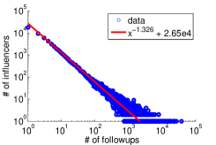
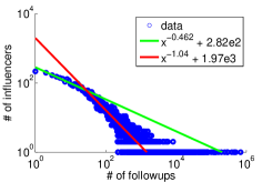
Figure 1: Frequency distribution of number of followups in Flixster (left) and Twitter (right). Both axes are in log scale.

V-B Qualitative Analysis

Through qualitative analysis, we mainly seek to validate our problem settings, approach and algorithm. But we note the limitations imposed by the public datasets available. In Twitter dataset, we know the identity of the influencers. We can thus validate our approach by checking if the distribution of influence is along the expected lines. On the other hand, in Flixster dataset, we do not know the identity of the influencers, but have the access to both user and action attributes. Thus, in this case, we can examine the benefits of incorporating followers’ demographics (as we saw in the example shown in Table I).

TABLE III: Kali: User with 2nd most followups. $k=6$, $k=3$.

			Actions	Followers	Followups
			(2.8k)	(93)	(27.0k)
female	comedy	pre-1997	550	62	2.8k
	thriller	action	549	62	3.1k
	drama	len:long	475	62	2.8k
		len:med	483	62	2.1k
male	thriller	rated:R	687	28	2.6k
	age:25-34	pre-1997	1.4k	13	2.3k
Total Coverage:					51.4%

TABLE IV: Julie: User with 3rd most followups. $k=6$, $l=3$.

			Actions	Followers	Followups
			(1.8k)	(73)	(23.5k)
female	pre-1997	comedy	401	63	4.3k
		rat:7-10	317	63	3.9k
	1998-2002	comedy	238	63	3.2k
		drama	222	63	2.3k
	rated:R	thriller	446	63	3.7k
	PG-13	action	228	63	3.0k
Total Coverage:					68.7%

Formatting the Explanations. To avoid clutter, in the explanation tables, we do not mention the name of each attribute, and instead show its required value directly. For instance, consider the example in Table I. Here, “rated R” indicates the feature “maturity rating = rating R” and “thriller” implies “genre = thriller”. Similarly, we combine overlapping features (or predicates) from various explanations, to allow us to visualize the explanations in a tree structure. As an example, the features “rated R” and “thriller” are present in the first two explanations. We order the features in a manner that minimizes the repetition of the features in the explanations table.

Flixster. We take the top-3 influencers measured in terms of the number of followups they recieve, and apply our algorithm to generate explanations, for examining their influence distribution. The results are presented in Tables I, IV and IV. For simplicity, we refer to the top-3 users as Mike, Kali, and Julie, even though their identities in Flixster are unknown. Table II shows the complete set of movie features. For users, we have the features corresponding to attributes gender and age. The intent should be clear from the context.

While Table I shows the explanations for the most influential user (please see §I for more details about this user), Tables IV and IV show the explanations for users who received second and third most number of followups, Kali and Julie, respectively. Kali has rated 2.8K movies and received 27K followups from her 93 active followers. Julie has rated 1.8K movies and received 23.5K followups from her 73 active followers. While Kali’s explanations cover 51.4% of her followups, Julie’s explanations cover 68.7% of her followups.

Julie in particular is influential on female users, with all her followups in the explanations coming from female users. In fact, 63 among 73 of her followers are females. Finally, she is influential on all sorts of movies (on female users), ranging from comedy, drama, thiller and action. This implies that Julie might be a very good seed if the target market is females, perhaps better than the top-2 users whose influence is distributed among both males and females. This is the sort of insight that simply cannot be gained by viewing network values solely as a scalar! A final remark about the explanations found is that they are heterogeneous, in that they involve a mix of user and action features.

Twitter. We next analyze the results from Twitter dataset. Recall that we have user identities of key influencers in Twitter, which allows us to validate whether the topics on which these influencers reported to be influential by our algorithm are along the expected lines. This provides us a nice strategy to validate our problem settings and approach. For instance, we expect news accounts like New York Times (NYTimes) and CNN to be influential on topics like news, politics, media, etc, and individuals like Tim O’Reilly to be influential on news on software, tech, programming etc. Fortunately, we were able to generate a rich set of topics for tweets by expanding their mentioned URLs.

While we have the identity of the key influencers, for followers, we could not collect user attributes due to demographic data not being available through the API. Thus, our analysis is restricted to the action attributes, which consist of tweet topics. We focus on explanations of four influencers (Twitter accounts) – New York Times, National Geographic, CNN Breaking News and Tim O’Reilly, the results of which are presented in Tables VI, VI, VIII and VIII.

TABLE V: New York Times. $k=6$, $l=4$.

				Followups	Actions
				(246)	(12.5k)
news	nytimes	business	finance	32	745
			media	8	578
		culture	media	8	535
		journalism	photos	14	762
	politics	media	newspaper	79	8.5k
		nyt	journalism	43	4.2k
Total Coverage:					82.8%

TABLE VI: CNN breaking news. $k=6$, $l=3$.

			Actions	Followups
			(390)	(56.2k)
news	cnn	politics	295	39.8k
		business	10	1.9k
		breaking-news	75	13.3k
	media	tv	288	38.5k
	religion	chistianity	1	434
	magazine	sport	2	265
Total Coverage:				99.8%

TABLE VII: Tim O’Reilly. $k=6$, $l=3$.

			Actions	Followups
			(115)	(3.0k)
news	tech	software	11	410
		business	6	165
	media	politics	15	513
	magazine	science	3	113
development	programming	opensource	2	471
socialmedia	google	ping.fm	5	235
Total Coverage:				63.4%

TABLE VIII: National Geographic. $k=3$, $l=3$.

			Actions	Followups
			(262)	(23.6k)
science	nature	geography	116	12.8k
travel	national geographic	magazine	51	4.7k
		videos	38	2.3k
Total Coverage:				84.1%

Consider the news accounts NYTimes and CNN first. As we expect, both these accounts are influential on topics “news” and “politics”. Moreover, CNN is quite influential on topics like “tv” and “breaking news”, which do not appear in explanations of NYTimes. This makes sense as CNN is a television news channel, while NYTimes is a newspaper. Another interesting observation is that topics like “religion” and “christianity” appear in CNN explanations (but not in NYTimes explanations) indicating CNN airs programs about religion. In the sample we collected, CNN tweeted about religion and christianity only once, and received 434 retweets – much higher than the average of 56200/390 = 144 retweets per CNN tweet. Similarly, topics “journalism” and “photos” can be found in NYTimes explanations but not in CNN ones, while the topics “business” and “politics” can be found in both. Finally, it is interesting to note that these explanations are able to cover almost all the followups – 82.8% for NYTimes and 99.8% for CNN, suggesting that these accounts are followed mostly because of their news, politics, media etc, i.e., the topics represented in the explanations shown in these tables.

Next, in Table VIII, we show the explanations of influence of Tim O’Reilly, the founder of O’Reilly Media and a supporter of the free software and open source movements. Topics like “news, tech, media, software, open source, programming, development, google” etc. emerge as the topics of his influence, which agrees with our expectation. Finally, we explore the influence of the National Geographic Channel in Table VIII. This account is influential on “science, nature, geography travel” etc, again consistent with our expectations.

Above, we have seen that our algorithm outputs the features (topics) that we expect these well known accounts to be influential on. These observations clearly indicate that our problem settings and framework are valid and effective for the purpose of digging deep into the influence spread of influencers and providing explanations. When coupled with user features, as in the case of Flixster dataset, we are able to answer the questions we raised in §I: Where exactly does the influence of an influencer lie? How is it distributed? On what type of actions is an influencer influential? What are the demographics of its followers?

V-C Quantitative Analysis

We next focus on evaluating our algorithm from a quantitative perspective and compare our algorithm with other algorithms, in terms of the coverage achieved (the fraction of total followups), running time, and memory usage.

Algorithms Compared: We compare our algorithm, which we refer to as Greedy, with the following baselines.

Random: It selects the features randomly, with probability proportional to number of followups covered by each feature.

Most-Popular: It orders the features by their popularity, i.e., number of followups they cover. Then, it picks the top $l$ features that have yet to be picked to build an explanation, this is repeated $k$ times. It is an intuitive algorithm, as the features which cover most followups can be seen as the representative set of features on which the given influencer is influential.

Exhaustive: It generates one explanation at a time, by exhaustively trying all possible combinations of features and picking the one that covers the maximum number of followups (which are not covered by previous explanations). Note that the number of possible combinations is ${|\mathcal{P}|\choose l}$, where $l$ is the number of features in one explanation. Thus, each explanation is an optimal one, i.e., the one with the maximum marginal coverage w.r.t. the previous set of explanations chosen. Since the objective function $\sigma:2^{2^{\mathcal{P}}}\rightarrow\mathbb{R}$ is monotone non-decreasing and submodular (see Thm. 2), the set of explanations obtained using this algorithm is an $(1-1/e)$-approximation to the optimal solution [18].

Thus, among the algorithms compared, algorithm Exhaustive provides the upper bound on the number of followups that can be possibly covered by the explanations generated. Because of its exhaustive nature, we expect the algorithm to be quite slow.

Unless otherwise stated, on each dataset, we take top-100 influencers with respect to number of followups they received. The algorithms are then run on all of 100 influencers, and the median is picked as the representative value for the comparison. We use median instead of mean, as it is more robust against outliers.

Coverage w.r.t. change in k: Figure 2 shows the variation in relative coverage achieved when $k$ is varied. Recall that $k$ denotes the number of explanations (table rows) generated. Relative coverage is defined as the fraction of followups that are covered. The parameter $l$ is fixed to 3 in Flixster and 5 in Twitter. As expected, the (relative) coverage increases with $k$, but not at the same rate for all algorithms. Our algorithm Greedy consistently performs just as well as Exhaustive, while beating both Random and Most-Popular by huge margins, on both the datasets. In fact, the performance of Greedy is almost indistinguishable from that of Exhaustive. For instance, on Flixster, with just 6 explanations, Greedy is able to cover 0.57 fraction of followups, compared to the fraction 0.58 achieved by Exhaustive. On the other hand, Most-Popular covers 0.25 fraction of followups and Random performs dismally, covering only 0.03 fraction of followups. Moreover, it is worth mentioning that the coverage achieved quickly saturates (on Flickr only) for both Most-Popular and Random, implying that increasing $k$ would not have helped achieve better coverage from these algorithms.

In case of Twitter, as we can observe, the coverage achieved, is in general higher, with Greedy covering up to 0.95 fraction of followups, again with 6 explanations. Recall, the longer an explanation (higher $l$) the smaller the coverage, in general. Despite this, the coverage achieved on Twitter with 6 longer explanations ($l=5$) is more than achieved on Flixster with 6 shorter explanations ($l=3$). This indicates that the influencers in Twitter are followed due to their niche. For example, news accounts like CNN and New York Times are mostly followed on topics like “news” and “politics” as we saw above. Once again, Greedy and Exhaustive significantly outperform other baselines while their performance is very close. The relative coverage of Random seems to grow sharply as $k$ increases but at $k=6$ it still performs poorly. The challenge is to cover as much as possible with as few but as detailed explanations as possible, and Greedy is found to rise to this challenge.

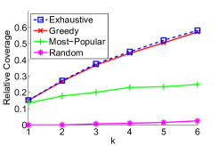
Figure 2: Coverage achieved from various algorithms w.r.t. variation in $k$ in Flixster (left) and Twitter (right). $l=3$ in Flixster and $l=5$ in Twitter.

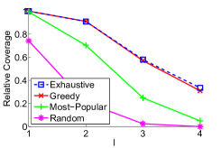
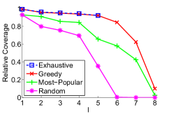
Figure 3: Coverage achieved from various algorithms w.r.t. variation in $l$ in Flixster (left) and Twitter (right). $k$ is fixed to 6.

Coverage w.r.t. change in l: In Figure 3, we show the variation in relative coverage when the parameter $l$, the number of features (table columns) per explanation, is changed. As expected, coverage decreases with the increase in $l$. Our Greedy algorithm continues to perform quite well. For instance, on Flixster, it covers 0.31 fraction of followups, compared to 0.05 and 0.00, the coverage achieved by Most-Popular and Random, respectively at $l=4$. Exhaustive on the other hand, covers 0.34 fraction of followups. We see a similar pattern in Twitter dataset as well. When $l=5$, Greedy covers 0.92 fraction of followups (same as 0.92 by Exhaustive), while the coverage from Most-Popular and Random is 0.66 and 0.35. Notice that Exhaustive took too long to complete for $l>5$ on Twitter.

Running Times and Memory Usage. Fig. 4 shows the running time of various algorithms, on both datasets. As can be seen, our Greedy algorithm is an order of magnitude faster than the optimal Exhaustive algorithm. For instance, on Flixster, when $k=6$ and $l=3$, while Greedy takes 26 ms to finish, Exhaustive finishes in 3,748 ms, that is, it takes 144 times longer than Greedy. The other algorithms – Most-Popular and Random are faster than Greedy as we foresaw earlier. They complete in 5 ms and 3 ms. Similarly, on Twitter, when $k=6$ and $l=5$, Exhaustive (finishes in 597 ms) is 18 times slower than Greedy (finishes in 32.5 ms). On the other hand, Most-Popular and Random take just 15 ms and 27 ms, respectively.

All the algorithms consume approximately the same amount of memory, up to a maximum of 446 MB and 2.92 GB on Flixster and Twitter, respectivly. This is because the memory usage primarily depends on the number of features and the number of followups they cover. To be precise, Greedy incurs additional space overhead on account of maintaining heaps of features, but this additional overhead is under 1 MB, which is negligible.

In sum, our Greedy algorithm performs essentially as well as Exhaustive algorithm in terms of coverage achieved, while being much more efficient in running time.

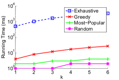
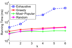
Figure 4: Running time comparison for various algorithms on Flixster with $l$ = 3 (left) and Twitter with $l$ = 5 (right).

VI Conclusions and Future Work

Ever since Domingos and Richardson [6] introduced the notion of network value of users in social networks, a lot of work has been done to identify influencers, community leaders, trendsetters etc. Work in this area has been further ignited since Kempe et al. [14] popularized influence maximization as a discrete optimization problem. Most of the current approaches largely work as a black box that just outputs a list of influencers or seeds, along with a scalar which is an estimate of the expected influence spread. A marketer would want to investigate the influence demographics of the seeds returned to her and validate them with her own independent survery and/or background knowledge. Motivated by this, our goal has been to open up the above black box and provide informative and crisp explanations for the influence distribution of influencers, thus allowing the marketer to drill down into a seed and address deeper analytic questions about what the seed is good for.

We formalized the above problem as that of finding up to $k$ explanations, each containing $l$ or more features, while maximizing the coverage. We showed the problem is not only NP-hard to solve optimally, but is NP-hard to approximate within any reasonable factor. Yet, exploiting the nice properties of the objective function, we developed a simple greedy algorithm. Our experiments on Flixster and Twitter datasets show the validity and usefulness of the explanations generated by our framework. Furthermore, they show that the greedy algorithm significantly outperforms several natural baselines. One of these is an exhaustive approximation algorithm that by repeatedly finding the explanation with the greatest marginal coverage gain achieves a (1-1/e)-approximation of the optimal coverage. However, our greedy algorithm achieves a coverage very close to that of the exhaustive approximation algorithm and is an order of magnitude or more faster. It is interesting to investigate how algorithms for mining maximum frequency item sets of a given cardinality (e.g., see [12]) can be leveraged for finding explanations with the maximum marginal gain.

Several interesting problems remain open. We give one example. Advertisers often like to target users in terms of properties like demographics, instead of targeting specific users. E.g., if we want to target female college grads in California, what would be an effective set of explanations that would describe the influence distribution of this demographic? How can we generate these explanations efficiently and validate them?

References

- [1] N. Agarwal, H. Liu, L. Tang, and P. S. Yu. Identifying the influential bloggers in a community. In WSDM, 2008.
- [2] E. Bakshy, J. M. Hofman, W. A. Mason, and D. J. Watts. Everyone’s an influencer: quantifying influence on twitter. In WSDM, 2011.
- [3] N. Barbieri, F. Bonchi, and G. Manco. Topic-aware social influence propagation models. In ICDM, 2012.
- [4] N. Barbieri, F. Bonchi, and G. Manco. Cascade-based community detection. In WSDM, 2013.
- [5] M. Cha et al. Measuring User Influence in Twitter: The Million Follower Fallacy. In ICWSM, 2010.
- [6] P. Domingos and M. Richardson. Mining the network value of customers. In KDD, 2001.
- [7] U. Feige. A threshold of for approximating set cover. J. ACM, 45(4):634–652, 1998.
- [8] M. Gomez-Rodriguez, J. Leskovec, and A. Krause. Inferring networks of diffusion and influence. In KDD, 2010.
- [9] A. Goyal, F. Bonchi, and L. V. S. Lakshmanan. Discovering leaders from community actions. In CIKM, 2008.
- [10] A. Goyal, F. Bonchi, and L. V. S. Lakshmanan. A data-based approach to social influence maximization. PVLDB, 5(1), 2011.
- [11] D. Gruhl, R. Guha, D. Liben-Nowell, and A. Tomkins. Information diffusion through blogspace. In WWW, 2004.
- [12] J. Han, J. Wang, Y. Lu, and P. Tzvetkov. Mining top-k frequent closed patterns without minimum support. In ICDM, pages 211–218, 2002.
- [13] M. Jamali and M. Ester. A matrix factorization technique with trust propagation for recommendation in social networks. In RecSys, 2010.
- [14] D. Kempe, J. M. Kleinberg, and É. Tardos. Maximizing the spread of influence through a social network. In KDD, 2003.
- [15] C. Lacave and F. J. Diez. A review of explanation methods for heuristic expert systems. Knowl. Eng. Rev., 19(2), 2004.
- [16] J. Leskovec et al. Cost-effective outbreak detection in networks. In KDD, 2007.
- [17] L. Liu, J. Tang, J. Han, M. Jiang, and S. Yang. Mining topic-level influence in heterogeneous networks. In CIKM, 2010.
- [18] G. L. Nemhauser, L. A. Wolsey, and M. L. Fisher. An analysis of approximations for maximizing submodular set functions. Mathematical Programming, 14(1):265–294, 1978.
- [19] F. Ricci, L. Rokach, B. Shapira, and P. B. Kantor, editors. Recommender Systems Handbook. Springer, 2011.
- [20] D. M. Romero, W. Galuba, S. Asur, and B. A. Huberman. Influence and passivity in social media. In WWW, 2011.
- [21] D. Saez-Trumper, G. Comarela, V. Almeida, R. Baeza-Yates, and F. Benevenuto. Finding trendsetters in information networks. In KDD, 2012.
- [22] M. Shieh, S. Tsai, and M. Yang. On the inapproximability of maximum intersection problems. Information Processing Letters, 2012.
- [23] J. Tang, J. Sun, C. Wang, and Z. Yang. Social influence analysis in large-scale networks. In KDD, 2009.
- [24] J. Weng, E.-P. Lim, J. Jiang, and Q. He. Twitterrank: finding topic-sensitive influential twitterers. In WSDM, 2010.
- [25] E. Xavier. A note on a maximum k-subset intersection problem. Information Processing Letters, 2012.