ABSTRACT: A discrete dynamical system in Euclidean $m$-space generated by the iterates of an asymptotically zero map $f$ , satisfying $\left|f(x)\right|\rightarrow 0$ as $\left|x\right|\rightarrow\infty$, must have a compact global attracting set $A$. The question of what additional hypotheses are sufficient to guarantee that $A$ has a minimal (invariant) subset $\mathfrak{A}$ that is a chaotic strange attractor is answered in detail for a few types of asymptotically zero maps. These special cases happen to have many applications (especially as mathematical models for a variety of processes in ecological and population dynamics), some of which are presented as examples and analyzed in considerable detail.

Keywords: Asymptotically zero maps, Strange attractors, Chaos, Lyapunov exponents, Fractal dimension, Pioneer and climax species

AMS Subject Classification 2010: 37D45; 37E99; 92D25; 92D40

1 Introduction

The identification and characterization of (chaotic) strange attractors in discrete dynamical systems is important for both theory and applications (see,e.g. [1, 2, 8, 9, 17, 20, 22, 23, 30, 31, 36, 37, 40, 41, 46] , but this is often very difficult to accomplish with the requisite mathematical rigor. Compelling evidence of the difficulty in proving the existence of strange attractors, even for relatively simple nonlinear maps, is provided by the pioneering work of Misiurewicz [26] on the Lozi map and that of Benedicks & Carleson [4] on the Hénon map, which in both cases - and especially the latter - required exceptionally lengthy, delicate and inspired analysis. In recent years, the basic ideas behind the proofs of these two landmark results in strange attractor theory have recently been extended and generalized in terms of a theory of rank one maps in an extraordinary series of papers by Wang & Young [42, 43, 45], the content of which gives striking confirmation of the exceptional complexity underlying characterizations of strange attractors for broad classes of discrete dynamical systems. Not only are the foundational results of rank one theory hard to prove, they also tend to be rather difficult to apply, as for example in Ott & Stenslund [27], which is closely related to results of Zaslavsky [47] and Wang & Young [44]. In light of this rather daunting rigorous strange attractor landscape, it is clear that there is a need for theory that is simpler to develop and apply for special classes of discrete dynamical systems of significant theoretical and applied interest. We make a start in this direction for some types among the class of discrete dynamical systems generated by what we call asymptotically zero maps, defined as follows: A map

$$f:\mathbb{R}^{m}\rightarrow\mathbb{R}^{m}$$

is asymptotically zero (AZ) if $\left|f(x)\right|\rightarrow 0$ as $\left|x\right|\rightarrow\infty$. We note that this includes exponentially decaying maps (cf. [10]) satisfying the property that $\left|f(x)\right|\leq Me^{-\left|x\right|}$ for some $M>0$ and all $x\in\mathbb{R}^{m}$, and it was our earlier work on these kinds of maps [21, 22] that inspired our present efforts - in fact, we were even able to formulate versions of the theorems that we prove here.

Our organization of the rest of this paper is as follows: In Section 2 we provide precise definitions of the concepts employed in the sequel and also prove some elementary dynamical properties of AZ maps. Then, in Section 3, we prove the existence of what we call radial strange attractors for smooth AZ maps possessing certain additional special properties. This is followed in Section 4 by a proof of the existence of another special kind of strange attractor, which we refer to as being of multihorseshoe (or trellis). In Section 5 we apply out theorems to several examples arising from various mathematical models and illustrate the strange attractors via simulation. We conclude our investigation in Chapter 6 by summarizing our findings, attempting to assess their impact and identifying some open problems they suggest. In addition, we also indicate some of our plans for related future research on strange attractors.

2 Preliminaries

Since there does not seem to universally accepted definitions for some of the key concepts that concern us, we shall describe exactly the ones we are using. For more standard definitions, we refer the reader to [1, 11, 17, 20, 28, 46]. First, we shall deal with chaos, which has several more or less equivalent characterizations.

Definition 1.

definition. Let $f:X\rightarrow X$ be a continuous self map of the metric space $X$. The map $f$, or the (semi) discrete dynamical system comprised of the iterates $f^{n}$ as $n$ ranges over the natural numbers $\mathbb{N}$, is chaotic if (1) $f$ is topologically transitive (or mixing), meaning that for every pair $U$, $V$ of open sets of $X$ there exists a $k\in\mathbb{N}$ such that $f^{k}(U)\cap V\neq\varnothing$ and (2) the set of periodic points of $f$, denoted as $Per(f)$, is dense in $X$.

This is essentially the prescription of Devaney [11] sans the property of sensitive dependence of iterates - common to most definitions of chaos. However, as shown by Banks et al. [3], sensitive dependence is implied by (1) and (2), which renders it redundant for our definition.

The definitions of an attractor and a strange attractor are also subject to various interpretations, so let us be specific.

Definition 2.

Let $f:X\rightarrow X$ be a continuous self map of the metric space $X$. A subset $A$ of $X$ is an attracting set of the map $f$ (or dynamical system generated by $f$) if it satisfies the following properties:

• • It is a nonempty, closed and (positively) invariant, i.e. $f(A)\subset A$.

  • There exists an open set $U$ containing $A$ such for every $x\in U$, $d\left(f^{n}(x),A\right)\rightarrow 0$ as $n\rightarrow\infty$.

Attracting sets with more complex structure and dynamics may be defined as follows:

Definition 3.

Let $f:X\rightarrow X$ be a continuous self map of the metric space $X$. A subset $A$ of $X$ is a  chaotic attracting set of the map $f$ $($or dynamical system generated by $f)$ if it satisfies the following properties:

• • It is an attracting set for $f$.

  • There is a nonempty closed invariant subset $A_{\ast}$ of $A$ such that the restriction $f_{|A_{\ast}}:A_{\ast}\rightarrow A_{\ast}$ is chaotic.

Definition 4.

Let $f:X\rightarrow X$ be a continuous self map of a subset of $\mathbb{R}^{m}$that is $C^{1}$ except possibly on finitely many $C^{1}$ submanifolds of $\mathbb{R}^{m}$ of dimensions less than $m$ $($a property we denote for convenience as $C^{1^{\ast}})$. A subset $A$ of $X$ is a semichaotic attracting set of the map $f$ $($or dynamical system generated by $f)$ if it satisfies the following properties:

• • It is a compact attracting set for $f$.

  • The restriction $f_{|A}:A\rightarrow A$ is continuous and $C^{1^{\ast}}$ and semichaotic in the sense that there is a nonempty, invariant subset $A_{\ast}$ of $A$ on which it is sensitively dependent on initial conditions, i.e.

    $$n^{-1}\log\left\|(f^{n})^{\prime}(x)\right\|=n^{-1}{\displaystyle\sum\nolimits_{k=1}^{n}}\log\left\|f^{\prime}\left(f^{k-1}(x)\right)\right\|\geq\ell>0\;\forall(x,n)\in A_{\ast}\times\mathbb{N},$$

    where $\left\|\cdot\right\|$denotes the standard norm of a linear map.

We note that it follows from the multiplicative ergodic theorem of Oseledec (see, e.g.[28, 46]) that the expression in (SCAS2) has a limit almost everywhere on $\mathbb{R}^{m}$, which represents the maximum Lyapunov exponent of the orbit initiating at $x$.

For an attractor, we add a bit more including a minimality requirement.

Definition 5.

Let $f:X\rightarrow X$ be a continuous self map of the metric space $X$. A subset $\mathcal{A}$ of $X$ is an attractor of the map $f$ $($or dynamical system generated by $f)$ if it satisfies the following properties:

• • It is a nonempty, closed and (positively) invariant, i.e. $f(\mathcal{A})\subset\mathcal{A}$.

  • There exists an open set $U$ containing $\mathcal{A}$ such for every $x\in U$, $d\left(f^{n}(x),\mathcal{A}\right)\rightarrow 0$ as $n\rightarrow\infty$.

  • It is minimal with respect to (i) and (ii), i.e. $\mathcal{A}$ has no proper subset with these properties.

A strange attractor is an attractor with additional properties including, for our purposes, chaotic dynamics.

Definition 6.

Let $f:X\rightarrow X$ be a continuous self map of the metric space $X$. A subset $\mathfrak{A}$ of $X$ is a chaotic strange attractor of the map $f$ $($or dynamical system generated by $f)$ if it satisfies the following properties:

• • It is an attractor.

  • The set is fractal, i.e. it has a noninteger fractal (Hausdorff) dimension.

  • The restriction $f|_{\mathfrak{A}}$ is chaotic.

The last property (CSA3) is not always included in definitions of strange attractors, and there are examples (such as in Grebogi et al. [16]) in which (CSA1) and (CSA2) are satisfied, but $f|_{\mathfrak{A}}$ is regular (nonchaotic).

For our purposes, it is convenient to define a weaker form of chaotic strange attractor.

Definition 7.

Let $f:X\rightarrow X$ be a continuous self map of a subset of $\mathbb{R}^{m}$. A subset $\mathfrak{A}$ of $X$ is a semichaotic strange attractor of the map $f$ (or dynamical system generated by $f$) if it satisfies the following properties:

• • It is an attractor.

  • The set is fractal, i.e. it has a noninteger fractal $($Hausdorff$)$ dimension.

  • The restriction $f|_{\mathfrak{A}}$ is $C^{1^{\ast}}$ and semichaotic.

2.1 Basic dynamical properties of AZ maps

Here we consider a couple of useful dynamical properties of continuous AZ maps that are easy to prove.

Lemma 8.

If $f:\mathbb{R}^{m}\rightarrow\mathbb{R}^{m}$ is a continuous AZ map, $f$ and all of its iterates $f^{n}$, $n>1$, have fixed points in the compact ball $B_{R}(0):=\{x\in\mathbb{R}^{m}:\left|x\right|\leq R\}$ for $R>0$ sufficiently large.

Proof.

As $\left|f\right|$ is continuous and $f$ is an AZ map, $\left|f\right|$ must achieve a maximum, say $M>0$, on $\mathbb{R}^{m}$. Accordingly $f^{n}(B_{R}(0))\subset B_{M}(0)\subset B_{R}(0)$ for every $R\geq M$ and $n\in\mathbb{N}$, which completes the proof in virtue of Brouwer’s fixed point theorem (see, e.g. [19]). ∎

Lemma 9.

Let $f$ and $M$ be as in Lemma 8 and its proof. Then $f$ has a compact globally attracting set defined as

$$A:={\displaystyle\bigcap\nolimits_{n=1}^{\infty}}f^{n}\left(B_{M}(0)\right)\subset B_{M}(0),$$ (1)

and this set must contain all of the fixed points of $f$ and its iterates.

Proof.

The set $A$ is the intersection of compact sets in $\mathbb{R}^{m}$, so it must be compact. Furthermore, it follows from Lemma 8 that it must be contained in $B_{M}(0)$ and contain all fixed points of $f$ and its iterates. Thus, the proof is complete. ∎

As an immediate corollary of the above lemmas, we obtain the following relation among the standard recurrence related sets (see e.g. [38]); namely, the periodic points $Per(f)$, the positive limit set $L_{+}(f)$ comprised of the closure of the union of all $\omega$-limit sets, the nonwandering set $\Omega(f)$ and the chain-recurrent set $R(f)$:

Corollary 10.

If $f$, $M$ and $A$ are as in Lemmas 8 and 9, then

$$Per(f)\subset L_{+}(f)=\Omega(f)=R(f)=A.$$ (2)

It follows from Lemma 9 that $A$ contains at least one minimal set (defined as a nonempty, closed invariant set with no proper subsets having the same properties). In the remaining sections we identify some cases when one of the minimal subsets is also a strange attractor. However, we first pause to prove a simple result about attractors that are at the other end of the complexity spectrum on which we are focusing, but have something of the radial essence of the first type of strange attractor we  shall analyze in the next section.

Lemma 11.

Suppose $f$, $M$ and $A$ are as in Lemmas 8 and 9, and satisfy the following additional properties: $(\mathrm{i})$ $f(0)=0$, and $(\mathrm{ii})$ $\left|f(x)\right|<\left|x\right|$ for all $0<\left|x\right|\leq R_{M}$, where $R_{M}:=\max\{\left|x\right|:\left|f(x)\right|=M\}$. Then the origin $\{0\}$ is a global attractor for $f$.

Proof.

Let $x_{0}$ be any initial point in $\mathbb{R}^{m}$. If $x_{0}$ or any of its $f$-iterates $x_{k}:=f^{k}(x_{0})$ is zero, we are done; so we assume that $x_{k}\neq 0$ for all $k\in\mathbb{N}$. It follows from the definitions and hypotheses that $0<\left|x_{k}\right|\leq R_{M}$ for all $k\geq 1$ and that $\left\{\left|x_{k}\right|:k\in\mathbb{N}\right\}$ is a strictly decreasing sequence of positive numbers. We need only show that $\left|x_{k}\right|\rightarrow 0$ as $k\rightarrow\infty$. If not, the monotone convergence property of the reals implies that the sequence converges to some number $a$ satisfying $0<a<R_{M}$. But this is impossible owing to the continuity of $\left|x\right|-\left|f(x)\right|$ and the compactness of $\{x\in\mathbb{R}^{m}:$ $a/2\leq\left|x\right|\leq(a+R_{M})/2\}$. Hence, we conclude that $\left|x_{k}\right|\rightarrow 0$ as $k\rightarrow\infty$, which completes the proof. ∎

3 Radial Strange Attractors

Our first result in this section is for a special class AZ maps.

Definition 12.

An AZ map $f:\mathbb{R}^{m}\rightarrow\mathbb{R}^{m}$ such that there exists a positive $R$ for which $f(x)=0$ whenever $\left|x\right|\geq R>0$ is said to be eventually zero (EZ).

If say the map was devised to for applications in population dynamics, an EZ model might be used in cases where all the species rapidly become extinct if the sum of all their members becomes too large. More specifically, the result that follows would apply to ecological dynamics models for what are called pioneer species that satisfy such an extinction property, while the subsequent theorem should be applicable to ecological dynamics involving climax species (see [14, 15, 21, 22, 34, 35, 39]).

3.1 Attractors for EZ maps expanding at the origin

If the origin is a source for an EZ map as is often the case for models of pioneer species, we have the following result.

Theorem 13.

Let $f:\mathbb{R}^{m}\rightarrow\mathbb{R}^{m}$ be a continuous EZ map, with $M$ and $R_{M}$ as in Lemma 11, satisfying the following additional properties:

• $f^{-1}\left(\{0\}\right)=\{0\}\cup Z$, where $Z=\{x\in\mathbb{R}^{m}:\left|x\right|\geq\zeta(x/\left|x\right|)>0$ $\}$, $\zeta:\mathbb{S}^{m-1}\rightarrow\mathbb{R}$ is a $C^{1}$ function satisfying $R_{M}<\zeta(u)<M$ for all $u\in\mathbb{S}^{m-1}$ and $\mathbb{S}^{m-1}:=\{u\in\mathbb{R}^{m}:\left|u\right|=1\}$ is the unit $(m-1)$-sphere.

• The set $S_{\ast}:=f^{-1}\left(Z\right)$ is an $(m-1)$-spherical shell of the form

  $$S_{\ast}=\{x\in\mathbb{R}^{m}:0<\alpha(x/\left|x\right|)\leq\left|x\right|\leq\beta(x/\left|x\right|)\},$$

  where $\alpha,\beta:\mathbb{S}^{m-1}\rightarrow\mathbb{R}$ are positive $C^{1}$ functions such that $0<\beta(u)-\alpha(u)<\zeta(u)$ for all $u\in\mathbb{S}^{m-1}$.

• $f$ is $C^{1}$ in $D:=\{0\}\cup\{x\in\mathbb{R}^{m}:0<\left|x\right|<\zeta\left(x/\left|x\right|\right)\}$ and the derivative $f^{\prime}(x)$ is invertible at every $x\in D\smallsetminus\{x\in\mathbb{R}^{m}:0<\alpha(x/\left|x\right|)<\left|x\right|<\beta(x/\left|x\right|)\}$.

• The radial derivative denoted as $\partial_{r}\left|f\right|$ and defined as

  $$\partial_{r}\left|f\right|(x):=\left\langle\nabla\left|f\right|(x),x/\left|x\right|\right\rangle,$$

  when it exists, is such that there are numbers $\lambda,\mu$ with $\mathfrak{M}/\mathfrak{m}<\lambda<\mu$ for which $\lambda\leq\partial_{r}\left|f\right|(x)\leq\mu$ for every $x\in\{x\in\mathbb{R}^{m}:0<\left|x\right|\leq\alpha\left(x/\left|x\right|\right)\}$ and $-\mu\leq\partial_{r}\left|f\right|(x)\leq-\lambda$ whenever $x\in\{x\in\mathbb{R}^{m}:\beta\left(x/\left|x\right|\right)\leq\left|x\right|<\zeta\left(x/\left|x\right|\right)\}$. Here $\mathfrak{m}:=\min\{\alpha(u):u\in\mathbb{S}^{m-1}\},\mathfrak{M}:=\max\{\beta(u):u\in\mathbb{S}^{m-1}\}$ and $\nabla$ is the usual gradient operator.

Then

$$\Lambda:=\bar{D}\smallsetminus{\displaystyle\bigcup\nolimits_{n=1}^{\infty}}f^{-n}\left(\mathring{S}_{\ast}\right),$$ (3)

is a compact semichaotic strange global attracting set having $m$-dimensional Lebesgue measure zero, where $\bar{E}$ and $\mathring{E}$ denote the closure and interior, respectively, of the set $E$.

Proof.

It follows directly from the hypotheses and construction that $\Lambda$ is a compact global attracting set for $f$. Moreover, excepting the origin, it is essentially a two-component Cantor set (generated by $(m-1)$-spherical shells rather than intervals). Consequently, it must be a fractal set. More precisely, we see from the properties (in particular (iv)) of the map that we have

$$f^{-1}\left(S_{\ast}\right)=S_{0}\cup S_{1},$$

where the union is disjoint and both $S_{0}$ and $S_{1}$ are open $(m-1)$-spherical shells such that $S_{i}\subset\mathring{\Sigma}_{i}$, $i=0,1$, where

$$\Sigma_{0}:=\{0\}\cup\{x\in\mathbb{R}^{m}:0<\left|x\right|\leq\alpha\left(x/\left|x\right|\right)\}\text{ and }\Sigma_{1}:=\{x\in\mathbb{R}^{m}:\beta\left(x/\left|x\right|\right)\leq\left|x\right|\leq\zeta\left(x/\left|x\right|\right)\},$$

and we note that we have the partition

$$\bar{D}=\Sigma_{0}\cup S_{\ast}\cup\Sigma_{1}.$$

Repeating the pre-imaging operation on the open $(m-1)$-spherical shells, we obtain the partitions of open cells

$$f^{-1}\left(S_{0}\right)=S_{00}\cup S_{01}\text{ and }f^{-1}\left(S_{1}\right)=S_{10}\cup S_{11},$$

where $S_{0i},S_{1i}\subset\mathring{\Sigma}_{0i}$, $i=0,1$, and the sets are defined by the following partitions written in what is obviously meant by ‘radial order’

$$\Sigma_{0}=\Sigma_{00}\cup S_{0}\cup\Sigma_{01}\text{ and }\Sigma_{1}=\Sigma_{10}\cup S_{1}\cup\Sigma_{11}.$$

But this is, if continued, just the standard inductive construction for the Cantor set, so we obtain the disjoint union representation

$$\Lambda={\displaystyle\bigvee\nolimits_{s\in 2^{\mathbb{N}}}}\Sigma_{s},$$

where, as usual, $2^{\mathbb{N}}$ is the set of maps $s:\mathbb{N}\rightarrow\{0,1\}$, which can, of course be identified with the set of binary sequences

$$\{.a_{1}a_{2}a_{3}\ldots:a_{i}=0\text{ or }1\text{ for all }i\in\mathbb{N}\}.$$

Whence, it follows directly from a simple argument, based on sliding the shell boundaries along rays, that $\Lambda$ is homeomorphic and actually $C^{1}$ diffeomorphic on the complement of the origin to a fractal ‘cone’ pinched at the origin; namely

$$\Lambda\cong\left(\mathbb{S}^{m-1}\times C\right)/\mathbb{S}^{m-1}\times 0,$$ (4)

where $\cong$ denotes homeomorphic, $C$ is a standard two-component Cantor set on the unit interval $[0,1]$, and the space on the right above has the usual quotient topology. For convenience, we shall refer to (4) as the Cantor cone of $\ \mathbb{S}^{m-1}$. This conclusively shows that the attracting set is fractal. As for the sensitive dependence on initial conditions, this is an immediate consequence of the construction of $\Lambda$ and (iv). Indeed, we compute that for all $x\in D$

$$n^{-1}\log\left\|(f^{n})^{\prime}(x)\right\| =n^{-1}{\displaystyle\sum\nolimits_{k=1}^{n}}\log\left\|f^{\prime}\left(f^{k-1}(x)\right)\right\|$$

$$\geq n^{-1}{\displaystyle\sum\nolimits_{k=1}^{n}}\log\left|\partial_{r}\left|f\right|(f^{k-1}(x))\right|\geq\log\lambda>0,$$

so $\lim\inf n^{-1}\log\left\|(f^{n})^{\prime}(x)\right\|>0$, and the sensitive dependence is established, which completes the proof. ∎

Observe that the maps described in the above theorem all have what one might call a degenerate snap-back repeller at the origin (c.f. Marotto [23] and Chen & Aihara [9]), which might be related to their chaotic nature in some as yet to be determined way.

We note here one can approximate the fractal dimension of the attractor in the above theorem. Using standard fractal techniques (see e.g.[13]), a straightforward but more laborious argument than we care to go into here yields the following estimate for the Hausdorff dimension $\dim_{H}$:

$$m-1+\log 2/\log(1+\mu)\leq\dim_{H}\left(\Lambda\right)\leq m-1+\log 2/\log(1+\lambda).$$ (5)

If we examine the proof of Theorem 13, more information on the structure of the restriction of the map to the attracting set can be readily obtained. First, we may recast the Cantor cone (4) in the form

$$\Lambda\cong\left(\mathbb{S}^{m-1}\times 2^{\mathbb{N}}\right)/\left(\mathbb{S}^{m-1}\times 0\right),$$ (6)

where $2^{\mathbb{N}}$ is given the metric topology generated by

$$d_{B}\left(s,\tilde{s}\right):={\displaystyle\sum\nolimits_{n=1}^{\infty}}2^{-n}\left|s(n)-\tilde{s}(n)\right|.$$

Then, by making fairly obvious modifications of a standard argument, used for example in studying the Smale horseshoe via symbolic dynamics (see, e.g. [38]), it is a straightforward matter to verify the following result.

Corollary 14.

The hypotheses of Theorem 13 implies that $f$ is conjugate on $\Lambda$ to a map of the form

$$\hat{f}:\left(\mathbb{S}^{m-1}\times 2^{\mathbb{N}}\right)/\left(\mathbb{S}^{m-1}\times 0\right)\rightarrow\left(\mathbb{S}^{m-1}\times 2^{\mathbb{N}}\right)/\left(\mathbb{S}^{m-1}\times 0\right),$$

where

$$\hat{f}(x,s):=\left(\nu(x,s),\sigma(s)\right),$$

$\sigma$ is the shift map $($with $\sigma(.a_{1}a_{2}a_{3}\ldots)=(.a_{2}a_{3}a_{4}\ldots))$ and $\nu$ is a continuous map.

If we have additional information concerning the behavior of the map on the spherical shell comprising the global attractor given by (3) in Theorem 13, it is sometimes possible to prove that one has in fact a true chaotic strange attractor. An example of such a result is the following, which clearly can be readily generalized.

Corollary 15.

Suppose in addition to the hypotheses of Theorem 13, $f$ satisfies the following property: There exists a finite set of $C^{1}$ curves $\{\gamma_{1},\gamma_{2},\ldots,\gamma_{k}\}\subset\bar{D}$ such that:

• Each curve begins at $x=0$ and ends at a distinct point of the boundary $\partial\bar{D}=\{x\in\mathbb{R}^{m}:x=\zeta\left(x/\left|x\right|\right)\}$ of $\bar{D}.$

• The curves are all transverse to $\partial S_{\ast}=$ $\{x\in\mathbb{R}^{m}:x=\alpha\left(x/\left|x\right|\right)\}\cup\{x\in\mathbb{R}^{m}:x=\beta\left(x/\left|x\right|\right)\}.$

• $f(\gamma_{j})=\gamma_{j+1}$, $1\leq j\leq k-1$, and $f(\gamma_{k})=\gamma_{1}$.

• The set $E:=\gamma_{1}\cup\gamma_{2}\cup\cdots\cup\gamma_{k}$ is conically attracting in the sense that there is a conical open set (pinched at the origin) $W$ such that $d(f^{n}(x),E)\rightarrow 0$ as $n\rightarrow\infty$ whenever $x\in E.$

Then

$$\mathfrak{A}:=\Lambda\cap E,$$

where $\Lambda$ is as in (3), is a chaotic strange global attractor.

Proof.

It follows at once from the hypotheses and Theorem 13 that $\mathfrak{A}$ is a semichaotic strange global attractor. Consequently, it suffices to prove that $f$ restricted to $\mathfrak{A}$, denoted as $g:=$ $f|_{\mathfrak{A}}$, which can be identified with its conjugate described in Corollary 14, is both topologically transitive and that its periodic points are dense. We first prove that given any $x,\tilde{x}\in\mathfrak{A}$ and any open neighborhood $U$ of $x$, there is a point $\breve{x}\in U$ and an $N\in\mathbb{N}$ such that $g^{N}(\breve{x})=\tilde{x}$, which clearly implies topological transitivity. Let $x\in\gamma_{i}\cap\Lambda$ belong to the $(m-1)$-spherical shell corresponding to $s=.a_{1}a_{2}\ldots$and $\tilde{x}\in\gamma_{j}\cap\Lambda$ belong to the $(m-1)$-spherical shell corresponding to $\tilde{s}=.\tilde{a}_{1}\tilde{a}_{2}\ldots$. Define $q$ to be the least nonnegative integer such that $g^{q}(\gamma_{i})=\gamma_{j}$ and note that it follows from (c) that $g^{lk+q}(\gamma_{i})=\gamma_{j}$ for every nonnegative integer $l$. Given any $\epsilon>0$, we can obviously choose $l$ so large that $d_{B}(s,\breve{s})<\epsilon$, where

$$\breve{s}:=.a_{1}a_{2}\ldots a_{lk+q}\tilde{s}:=.a_{1}a_{2}\ldots a_{lk+q}\tilde{a}_{1}\tilde{a}_{2}\ldots,$$

and then define $\breve{x}$ to be the intersection of $\gamma_{i}$ with the $(m-1)$-spherical shell associated to $\breve{s}$. Clearly, by selecting $\epsilon$ sufficiently small, we can guarantee that $\breve{x}\in U$. But it follows from our construction that $\sigma^{lk+q}(\breve{s})=\tilde{s}$, so $g^{lk+q}(\breve{x})=\tilde{x}$ and the topological transitivity follows. The density of the periodic points can be readily verified by a straightforward modification of the transitivity argument. To wit, let $x\in\gamma_{i}\cap\Lambda$ belong to the $(m-1)$-spherical shell corresponding to $s=.a_{1}a_{2}\ldots$. Given any $\epsilon>0$, select $l$ so large that $d_{B}(s,\overline{.a_{1}\ldots a_{lk}})<\epsilon$, where $\overline{.a_{1}\ldots a_{lk}}$ is the binary sequence formed by successively concatenating the finite sequence $.a_{1}a_{2}\ldots a_{lk}$ with itself, i.e.

$$\overline{.a_{1}\ldots a_{lk}}:=.a_{1}a_{2}\ldots a_{lk}a_{1}a_{2}\ldots a_{lk}\ldots.$$

It is easy to see that $\overline{.a_{1}\ldots a_{lk}}$ is a periodic point of period $lk$ for the shift map $\sigma$ and if we select $\bar{x}$ to be the point of $\gamma_{i}$ on the $(m-1)$-spherical shell corresponding to $\overline{.a_{1}\ldots a_{lk}}$, then $g^{lk}(\bar{x})=\bar{x}$, so the proof is complete since $\epsilon$ is arbitrary. ∎

3.2 Attractors for AZ maps contracting at the origin

When the origin is a sink rather than a source, as it typically is for models of populations comprised entirely of climax species, we can relax the extermination requirement of Theorem 13 and obtain analogous results concerning strange attractor for globally $C^{1}$ maps. An example is the following.

Theorem 16.

Suppose $f:\mathbb{R}^{m}\rightarrow\mathbb{R}^{m}$ is a $C^{1}$ EZ map, with $M$ and $R_{M}$ as in Lemma 11, for which the following properties obtain:

• $f^{-1}\left(\{0\}\right)=\{0\}$, $\left\|f^{\prime}(0)\right\|<1$ and $\{0\}$ has a basin of attraction of the form

  $$\mathcal{B}(0):=\{x\in\mathbb{R}^{m}:0\leq\left|x\right|<\alpha_{0}(x/\left|x\right|)\},$$

  where $\alpha_{0}:\mathbb{S}^{m-1}\rightarrow\mathbb{R}$ is a positive $C^{1}$ function and $f^{-1}\left(\mathcal{B}(0)\right)$ is a semi-infinite $(m-1)$-spherical shell of the form

  $$Z:=\{x\in\mathbb{R}^{m}:\zeta\left(x/\left|x\right|\right)<\left|x\right|\},$$

  where $\zeta:\mathbb{S}^{m-1}\rightarrow\mathbb{R}$ is a $C^{1}$ function satisfying $R_{M}<\zeta(u)<M$ for all $u\in\mathbb{S}^{m-1}$.

• The set $S_{\ast}:=f^{-1}\left(\bar{Z}\right)$ is an $(m-1)$-spherical shell of the form

  $$S_{\ast}=\{x\in\mathbb{R}^{m}:0<\alpha(x/\left|x\right|)\leq\left|x\right|\leq\beta(x/\left|x\right|)\},$$

  where $\alpha,\beta:\mathbb{S}^{m-1}\rightarrow\mathbb{R}$ are positive $C^{1}$ functions such that $0<\beta(u)-\alpha(u)<\zeta(u)$ for all $u\in\mathbb{S}^{m-1}$.

• $f^{\prime}(x)$ is invertible at every $x\in D\smallsetminus\{x\in\mathbb{R}^{m}:0<\alpha(x/\left|x\right|)<\left|x\right|<\beta(x/\left|x\right|)\}$.

• The radial derivative denoted as $\partial_{r}\left|f\right|$ and defined as

  $$\partial_{r}\left|f\right|(x):=\left\langle\nabla\left|f\right|(x),x/\left|x\right|\right\rangle,$$

  when it exists, is such that there are numbers $\lambda,\mu$ with $\mathfrak{M}/\mathfrak{m}<\lambda<\mu$ for which $\lambda\leq\partial_{r}\left|f\right|(x)\leq\mu$ for every $x\in\{x\in\mathbb{R}^{m}:0<\left|x\right|\leq\alpha\left(x/\left|x\right|\right)\}$ and $-\mu\leq\partial_{r}\left|f\right|(x)\leq-\lambda$ whenever $x\in\{x\in\mathbb{R}^{m}:\beta\left(x/\left|x\right|\right)\leq\left|x\right|<\zeta\left(x/\left|x\right|\right)\}$. Here $\mathfrak{m}:=\min\{\alpha(u):u\in\mathbb{S}^{m-1}\},\mathfrak{M}:=\max\{\beta(u):u\in\mathbb{S}^{m-1}\}$ and $\nabla$ is the usual gradient operator.

Then

$$\Gamma:=\{0\}\vee\Gamma_{C},$$ (7)

where

$$\Gamma_{C}:=\bar{D}\smallsetminus{\displaystyle\bigcup\nolimits_{n=1}^{\infty}}f^{-n}\left(\mathring{S}_{\ast}\right),$$

is a compact semichaotic strange minimal global attracting set having $m$-dimensional Lebesgue measure zero.

Proof.

As the proof of this result is completely analogous to that of Theorem 13, we need only sketch the argument. Again we immediately deduce from the hypotheses and construction that $\Gamma$ is a compact global attracting set for $f$. Moreover, excepting the origin, it is a two-component Cantor set (generated by $(m-1)$-spherical shells rather than intervals) contained in $\{x\in\mathbb{R}^{m}:\alpha_{0}(x/\left|x\right|)\leq\left|x\right|\leq\zeta(x/\left|x\right|)\}$. Consequently, it must be a fractal set. More precisely, we see from the properties (in particular (iv)) of the map that we have

$$f^{-1}\left(S_{\ast}\right)=S_{0}\cup S_{1},$$

where the union is disjoint and both $S_{0}$ and $S_{1}$ are open $(m-1)$-spherical shells such that $S_{i}\subset\mathring{\Sigma}_{i}$, $i=0,1$, where

$$\Sigma_{0}:=\{0\}\cup\{x\in\mathbb{R}^{m}:\alpha_{0}\left(x/\left|x\right|\right)\leq\left|x\right|\leq\alpha\left(x/\left|x\right|\right)\}\text{ and }\Sigma_{1}:=\{x\in\mathbb{R}^{m}:\beta\left(x/\left|x\right|\right)\leq\left|x\right|\leq\zeta\left(x/\left|x\right|\right)\},$$

and we note that we have the partition

$$\bar{D}=\Sigma_{0}\cup S_{\ast}\cup\Sigma_{1}.$$

Repeating the pre-imaging operation on the open $(m-1)$-spherical shells, we obtain the partitions of open cells

$$f^{-1}\left(S_{0}\right)=S_{00}\cup S_{01}\text{ and }f^{-1}\left(S_{1}\right)=S_{10}\cup S_{11},$$

where $S_{0i},S_{1i}\subset\mathring{\Sigma}_{0i}$, $i=0,1$, and the continuing, we obtain in a manner quite like that in the proof of Theorem 13 the Cantor set representation

$$\Gamma_{C}={\displaystyle\bigvee\nolimits_{s\in 2^{\mathbb{N}}}}\Sigma_{s}\subset\bar{D}.$$

Whence, by again sliding the shell boundaries along rays, we see that $\Gamma_{C}$ is homeomorphic and actually $C^{1}$ diffeomorphic with

$$\Gamma_{C}\cong\mathbb{S}^{m-1}\times C,$$ (8)

where $\cong$ denotes homeomorphic and $C$ is a standard two-component Cantor set on the unit interval $[0,1]$. This conclusively shows that the attracting set $\{0\}\cup$ $\Gamma_{C}$ is fractal. The sensitive dependence is an immediate consequence of the construction of $\Gamma_{C}$ and (iv). Indeed, we compute that for all $x\in D$

$$n^{-1}\log\left\|(f^{n})^{\prime}(x)\right\| =n^{-1}{\displaystyle\sum\nolimits_{k=1}^{n}}\log\left\|f^{\prime}\left(f^{k-1}(x)\right)\right\|$$

$$\geq n^{-1}{\displaystyle\sum\nolimits_{k=1}^{n}}\log\left|\partial_{r}\left|f\right|(f^{k-1}(x))\right|\geq\log\lambda>0,$$

so $\lim\inf n^{-1}\log\left\|(f^{n})^{\prime}(x)\right\|>0$, which implies sensitive dependence, and the proof is complete. ∎

The approximate value for the Hausdorff dimension (5) also applies here, and there are rather obvious analogs (where the origin is a sink rather than a source) of Corollaries 14 and 15 for Theorem 16. We only state these results, since their proofs are essentially the same mutatis mutandis as those given for their analogs.

Corollary 17.

The hypotheses of Theorem 16 implies that $f$ is conjugate on $\Gamma$ to a map of the form

$$\hat{f}:\left[\{0\}\vee\left(\mathbb{S}^{m-1}\times 2^{\mathbb{N}}\right)\right]/\left(\mathbb{S}^{m-1}\times 0\right)\rightarrow\left[\{0\}\vee\left(\mathbb{S}^{m-1}\times 2^{\mathbb{N}}\right)\right]/\left(\mathbb{S}^{m-1}\times 0\right),$$

where

$$\hat{f}(0):=0\text{ and }\hat{f}(x,s):=\left(\nu(x,s),\sigma(s)\right)\text{ for }x\neq 0,$$

$\sigma$ is the shift map $($with $\sigma(.a_{1}a_{2}a_{3}\ldots)=(.a_{2}a_{3}a_{4}\ldots))$ and $\nu$ is a continuous map.

Corollary 18.

Suppose in addition to the hypotheses of Theorem 16, $f$ satisfies the following property: There exists a finite set of $C^{1}$ curves $\{\gamma_{1},\gamma_{2},\ldots,\gamma_{k}\}\subset\bar{D}$ such that:

• Each curve begins at $x=0$ and ends at a distinct point of the boundary $\partial\bar{D}=\{x\in\mathbb{R}^{m}:x=\zeta\left(x/\left|x\right|\right)\}$ of $\bar{D}.$

• The curves are all transverse to $\partial S_{\ast}=$ $\{x\in\mathbb{R}^{m}:x=\alpha\left(x/\left|x\right|\right)\}\cup\{x\in\mathbb{R}^{m}:x=\beta\left(x/\left|x\right|\right)\}.$

• $f(\gamma_{j})=\gamma_{j+1}$, $1\leq j\leq k-1$, and $f(\gamma_{k})=\gamma_{1}$.

• The set $E:=\gamma_{1}\cup\gamma_{2}\cup\cdots\cup\gamma_{k}$ is conically attracting.

Then

$$\mathfrak{A}:=\Gamma\cap E,$$

where $\Gamma$ is as in (7), is a chaotic strange minimal global attractor.

A few remarks are in order before we move on to a discussion of another - very different - type of strange attractor. In Theorem 16, the origin is actually a global metric attractor (see, e.g. Milnor [24, 25]) because $\Gamma_{C}$ has $m$-dimensional Lebesgue measure zero, but the minimal global attractor is indeed $\Gamma$. The basin of attraction is riddled in a measure zero sense (c.f. [8]). In applications, the model maps frequently leave all of the coordinate axes invariant (such as in [10, 18, 21, 22, 34, 35, 39]) in which case there are obvious versions of the above strange attractor results for maps restricted to $x_{1},\ldots,x_{m}\geq 0$, for example.

4 Multihorseshoe (Trellis) Strange Attractors

In this section we describe another type of attractor generated by one or more horseshoes associated to hyperbolic fixed or periodic points. These attractors apparently were first studied in reasonable detail (for planar maps with an emphasis on characterizing the stable-unstable manifold connections of neighboring horseshoes) by Easton [12], who seems also to have coined the name “trellis” to describe their structure. They can often be found in the dynamics of AZ maps, but they may occur for more general smooth maps as well. It is convenient to introduce the following concept.

Definition 19.

Let $f:X\rightarrow X$ be a $C^{1}$ self map of the $m$-dimensional $C^{1}$ manifold $X$. A subset $H$ of $X$ is an attracting 1$\boldsymbol{\times}$(m-1)-horseshoe(at p) for $f$ if the following properties obtain:

• • There is a $C^{1}$ diffeomorphism $\varphi:H^{\ast}\rightarrow H$, where

    $$H^{\ast}:=C_{0}^{\ast}\cup Z^{\ast}\cup C_{1}^{\ast},$$

    with

    $$Z^{\ast} :=\left\{x\in\mathbb{R}^{m}:0\leq(x_{1}+2)^{2}+x_{2}^{2}+\cdots+x_{m-1}^{2}\leq 4^{2},\;-1\leq x_{m}\leq 9\right\},$$

    $$C_{0}^{\ast} :=\left\{x\in\mathbb{R}^{m}:0\leq(x_{1}+2)^{2}+x_{2}^{2}+\cdots+(x_{m}+1)\leq 4^{2},\;x_{m}\leq-1\right\}\text{ and}$$

    $$C_{1}^{\ast} :=\left\{x\in\mathbb{R}^{m}:0\leq(x_{1}+2)^{2}+x_{2}^{2}+\cdots+(x_{m}-9)^{2}\leq 4^{2},\;x_{m}\geq 9\right\};$$

    so that defining $H:=\varphi\left(H^{\ast}\right)$, $Z:=\varphi\left(Z^{\ast}\right)$ and $C_{k}:=\varphi\left(C_{k}^{\ast}\right)$, $k=0,1$, we have the associated decomposition

    $$H=C_{0}\cup Z\cup C_{1}.$$

    We note that $H^{\ast}$ has both a $C^{\infty}$1-dimensional foliation $\mathcal{F}_{\mathrm{v}}^{\ast}$ comprised of leaves that are the intersections with $H^{\ast}$ of the lines of the form $x_{1},\ldots,x_{m-1}$ all constant, and a $C^{\infty}(m-1)$-dimensional foliation $\mathcal{F}_{\mathrm{h}}^{\ast}$ consisting of the intersections with $H^{\ast}$ of the hyperplanes $x_{m}=$ constant. These orthogonal foliations produce transverse $C^{1}$ foliations of $H$ defined by $\mathcal{F}_{\mathrm{v}}:=\varphi\left(\mathcal{F}_{\mathrm{v}}^{\ast}\right)$ and $\mathcal{F}_{\mathrm{h}}:=\varphi\left(\mathcal{F}_{\mathrm{h}}^{\ast}\right)$.

  • The map $f$ restricted to $H$ is injective, $f\left(H\right)\subset\mathring{H}$, and $f\left(C_{k}\right)\subset\mathring{C}_{0}$ for $k=0,1$.

  • The foliation $f\left(\mathcal{F}_{\mathrm{v}}\right)$ is transverse to the foliation $\mathcal{F}_{\mathrm{h}}$ in $Z$.

  • $f$ restricted to $C_{0}$ is a contraction mapping into $\mathring{C}_{0}$, and the unique fixed point $q$ in $\mathring{C}_{0}$ is an attractor with a basin of attraction containing $C_{0}$.

  • There is a further decomposition of $Z^{\ast}$ defined as

    $$Z^{\ast}=S_{0}^{\ast}\cup S_{1/2}^{\ast}\cup S_{1}^{\ast},$$

    where $S_{0}^{\ast}:=\{x\in Z^{\ast}:-1\leq x_{m}\leq 3\}$, $S_{1/2}^{\ast}:=\{x\in Z^{\ast}:3\leq x_{m}\leq 5\}$ and $S_{0}^{\ast}:=\{x\in Z^{\ast}:5\leq x_{m}\leq 9\}$, which naturally induces the decomposition of $Z$ given by

    $$Z=S_{0}\cup S_{1/2}\cup S_{1},$$

    where $S_{r}:=\varphi\left(S_{r}^{\ast}\right)$, $r=0,1/2,1$. For this decomposition, $f\left(S_{1/2}\right)\subset\mathring{C}_{1}$.

  • There is a hyperbolic fixed point (saddle) $p\in f\left(S_{0}\right)\cap S_{0}$ , corresponding to $\varphi\left(0\right),$with a $1-$dimensional unstable manifold $W^{u}(p)$ that is tangent at $p$ to the image under $\varphi$ of the leaf of $\mathcal{F}_{\mathrm{v}}$ through $p$ and an $(m-1)-$dimensional stable manifold $W^{s}(p)$ that is tangent at $p$ to the image under $\varphi$ of the leaf of $\mathcal{F}_{\mathrm{h}}$ through this point.

  • $f$ restricted to $Z$ is a contracting map along the leaves of $\mathcal{F}_{\mathrm{h}}$ with contraction coefficient $0<\lambda<1$, and an expanding map along the leaves of $f\left(\mathcal{F}_{\mathrm{v}}\right)$ with expansion coefficient $1<\mu$.

This rather verbose description of the criteria for the existence of attracting horseshoes is actually quite easy to apply and even easier to illustrate as shown in Fig. 1. With this nomenclature, we can now efficiently proceed to one of our main results on strange attractors, the proof of which includes a fairly straightforward extension of an argument used by Easton [12].

Theorem 20.

Let $f:E\rightarrow E$ be a $C^{1}$ self-map of a connected open subset of $\mathbb{R}^{m}$. If $f$ has an attracting $1\times(m-1)$ -horseshoe $H$ at $p\in E$, then

$$\mathfrak{A}:=\bigcap\nolimits_{n=1}^{\infty}f^{n}\left(H\right)=\overline{W^{u}(p)}$$

is a chaotic strange attractor of $f$ with a basin of attraction containing $H$, and $\mathfrak{A}$ is homeomorphic to

$$\left(K\times[0,1]\right)/\left(K\times\{0,1\}\right),$$ (9)

where $K$ is a two-component Cantor space and the usual quotient topology is used for the whole space.

Proof.

We first verify that $\mathfrak{A}$ is an attracting set. If $x\in H\smallsetminus\left(S_{0}\cup S_{1}\right)$, it follows from (AH2), (AH4) and (AH5) that $f^{2}(x)\in\mathring{C}_{0}$. Consequently, in virtue of (AH4), $f^{n}(x)\in\mathring{C}_{0}$ for all $n\geq 2$ and $f^{n}(x)\rightarrow q\in$ $\bigcap\nolimits_{n=1}^{\infty}f^{n}\left(H\right)=\overline{W^{u}(p)}$ as $n\rightarrow\infty$. Moreover, we readily infer that the only possible points $x$ in $H$ having iterates that do not converge to $\mathfrak{A}$ are those such that $f^{n}(x)\in S_{0}\cup S_{1}$ for all $n\geq 0$. But for points such as these, it follows from (AH3), (AH6) and (AH7) that $d\left(f^{n}(x),\mathfrak{A}\right)\leq c\lambda^{n}$ for all $n\in\mathbb{N}$, so $f^{n}(x)\rightarrow\mathfrak{A}$. Thus, $\mathfrak{A}$ is an attracting set that includes all of $H$ in its basin of attraction. In fact, the obvious fact that $\mathfrak{A}$ is indecomposable - which is probably most self-evident from its characterization as the closure of the unstable manifold of $p$ - shows that we have a minimal attracting set, which means that it is an attractor. To see that $\mathfrak{A}$ is fractal, one merely has to note that owing to (AH3) and the geometry of $f(H),$ its intersection with $Z$ is homeomorphic with $K\times[0,1]$, where $K$ is the two-component Cantor set in the statement of the theorem. As for the chaotic regimes of $f$ restricted to $\mathfrak{A}$, consider the subset defined as

$$\Lambda:=\mathfrak{A}\cap\left\{x\in H:f^{n}(x)\in S_{0}\cup S_{1}\right\}.$$

This is just the standard product of Cantor sets $K\times K$, which is $f$-invariant and on which it is well known (c.f. [1, 17, 28, 38, 46] and Theorem 13 and Corollary 14) that $f$ is conjugate to the shift map $\sigma:2^{\mathbb{Z}}\rightarrow 2^{\mathbb{Z}}$ defined as

$$\sigma\left(\{\cdots a_{-2}a_{-1}a_{0}.a_{1}a_{2}\cdots\}\right)=\{\cdots a_{-2}a_{-1}a_{0}a_{1.}a_{2}\cdots\}.$$

This map is topologically transitive and the periodic points are dense, so it follows that the map depends sensitively on initial points in $\Lambda$. The sensitive dependence can also be established directly from the properties of the attracting horseshoe; in fact, (AH6) and (AH7) implies that

$$\lim\inf{}_{n}n^{-1}\log\left\|(f^{n})^{\prime}(x)\right\|\geq\log\lambda>0$$

for all $x\in\Lambda$. It remains only to prove the representation of the attractor as the quotient space (9), which is obvious from the definition of the attracting horseshoe, so the proof is complete. ∎

It is likely that rank-one theory could also be used to prove the above theorem, but probably with considerably more effort than required for our proof. In addition, it appears that our approach might lead to some interesting generalizations that are beyond the scope of rank-one techniques.

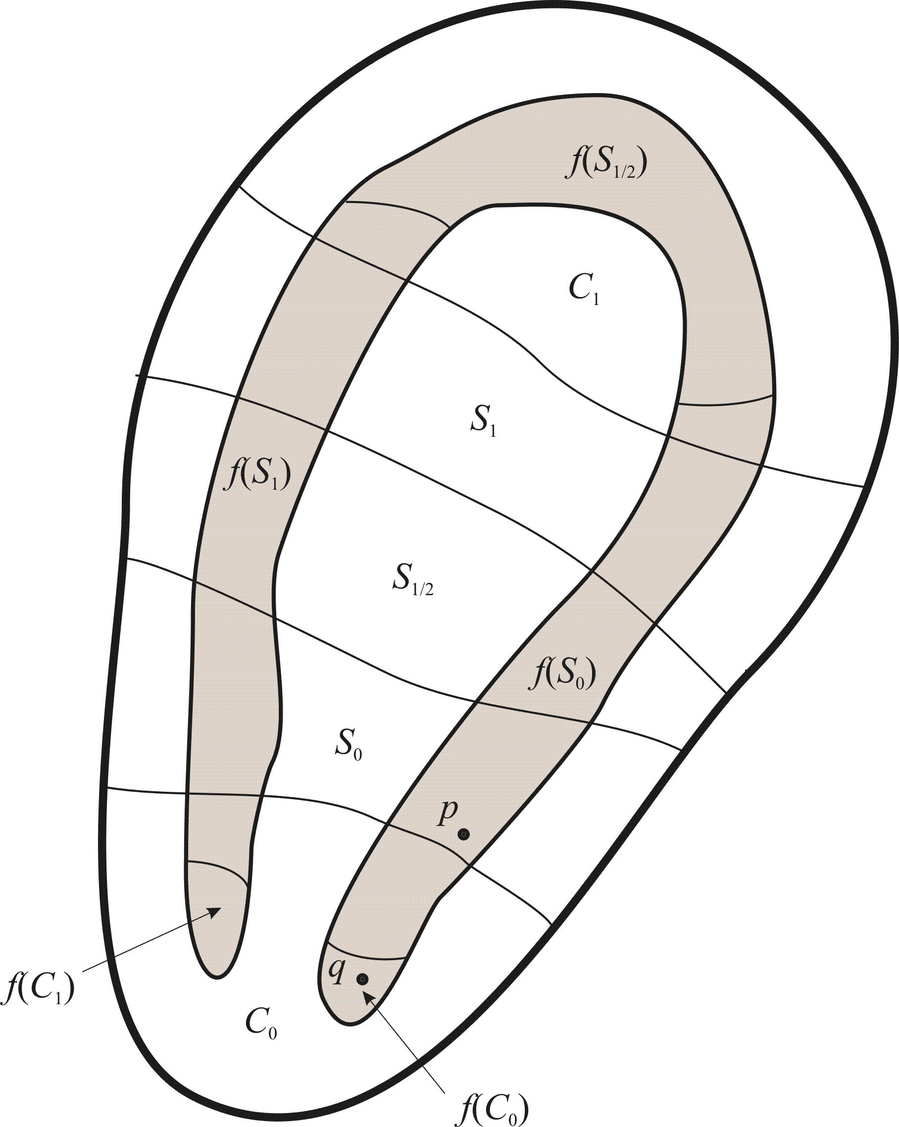
Figure 1: An attracting horseshoe

It is now an easy matter to generalize Theorem 20 to the case of multihorseshoe strange chaotic attractors (trellises), which tend to exemplify both great complexity and aesthetically interesting patterns, which we shall illustrate in the sequel. As the proof of the following results follows directly from Theorem 20, we leave it to the reader.

Theorem 21.

If $f:E\rightarrow E$ a $C^{1}$ self-map of a connected open subset of $\mathbb{R}^{m}$ that has a $k$-cycle of distinct points $\{p_{1},\ldots,p_{k}\}$ with $k>1$ and $f^{k}$ has an attracting $1\times(m-1)$ -horseshoe $H$ at one of the points $p$ in the cycle, then

$$\mathfrak{A}:=\overline{W^{u}(p)}\cup f\left(\overline{W^{u}(p)}\right)\cup\cdots\cup f^{k-1}\left(\overline{W^{u}(p)}\right)$$

is a chaotic strange attractor for $f$ with a basin of attraction containing $H\cup f\left(H\right)\cup\cdots\cup f^{k-1}\left(H\right).$

We remark that it is not difficult to find an analog of (5) to approximate the Hausdorff dimension of a single attracting horseshoe, from which one can deduce that the fractal dimension is just slightly larger than one if the contraction constant $\lambda$ in (AH7) is very small. On the other hand, even for relatively small contraction constants, interactions of the horseshoes (via intersections of respective unstable with stable manifolds)in trellises can produce strange attractors that appear to have fractal dimensions that are nearly equal to two for planar maps, as we shall illustrate in the simulation examples to be shown in the next section.

5 Applications and Examples

We shall now illustrate our strange attractor theorems via simulation. Our examples are chosen from well established discrete dynamical models for physical phenomena; in particular, those for predicting the evolution of ecological systems. For ease and clarity of visualization, we restrict the examples to maps of the plane. We begin our simulations with maps that have radial attractors

5.1 Radial attractor examples

Our first example involves the map $f:\mathbb{R}^{2}\rightarrow\mathbb{R}^{2}$ defined as

$$f(x_{1},x_{2})=f(x_{1},x_{2};a):=ae^{-x_{1}^{2}-x_{2}^{2}}\left(x_{1}\cos(2\pi\theta)-x_{2}\sin(2\pi\theta),x_{1}\cos(2\pi\theta)-x_{2}\sin(2\pi\theta)\right),$$ (10)

where $\theta$ is an irrational number (so that the rotational part is ergodic), is meant as an application of Theorem 13, but note that although this map is AZ, it is not EZ. This particular discrete dynamical system is of a type that has proven quite successful in modeling the evolution of several pioneer species cohabiting and competing in the same ecological environment. Fairly thorough descriptions of the properties of pioneer and climax species can be found in [14, 15, 21, 34, 35, 39].

Examples of radial type attractors for (10) that emerge for increasing values of $a$ for two different choices of $\theta$ (the golden mean $\phi:=(1+5)/2$ and the base of the natural logarithm $e$) are shown in Figs. 2 and 3. Reading the panels from left to right in these representations, the parameter $a$ starts at $2.7$ in the upper left-hand corner and increases by increments of $0.3$ until it reaches $6.0$ in the lower right-hand corner

Note how in each case the attractor essentially begins as a single invariant ellipse, then there is period-doubling to a two-cycle of ellipses that begins a period-doubling cascade that eventually leads to full-blown chaotic attractors when $a$ is sufficiently large (around $a=4.2$). For larger values of $a$ there is a parameter window (approximately $4.6<a<5$ ) in which the attractor appears to be regular, then for all larger values of the parameter ($a\geq 5.1$), one sees chaotic strange attractors of the kind described in Theorem 13.

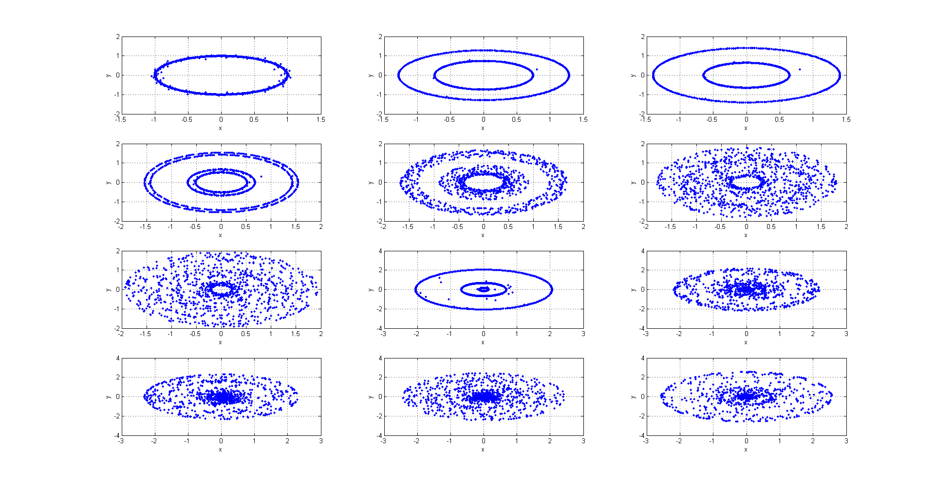
Figure 2: Changes in radial attractors for (10) with $\theta=\phi$ for $a=2.7,3,3.3,3.6,3.9,4.2,4.5,4.8,5.1,5.4,5.7,6.$

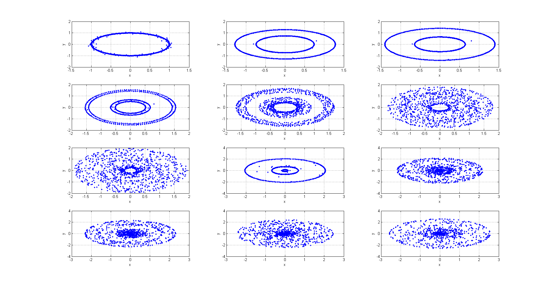
Figure 3: Changes radial attractors for (10) with $\theta=e$ for $a=2.7,3,3.3,3.6,3.9,4.2,4.5,4.8,5.1,5.4,5.7,6.$

5.2 Multihorseshoe attractor simulations

Next, we illustrate the case in which there are multihorseshoe attractors for different parameter values and note that the examples are drawn from models of pioneer-climax ecological dynamics. For our first example of this kind, the map $f:\mathbb{R}^{2}\rightarrow\mathbb{R}^{2}$ is

$$f(x_{1},x_{2})=f(x_{1},x_{2};a,b):=\left(x_{1}e^{a-0.8x_{1}-0.2x_{2}},x_{2}(0.2x_{1}+0.8x_{2})e^{b-0.2x_{1}-0.8x_{2}}\right).$$ (11)

Figure 4 shows the map (11) for $a=2.4$ and $b=2.5$ that follows intervals of slightly smaller values for which $f$ has a $6$-cycle of sinks, which develop nearby saddles and associated attracting horseshoes when $a$ and $b$ are sufficiently large, as illustrated in Fig. 5 for $a=b=3$.

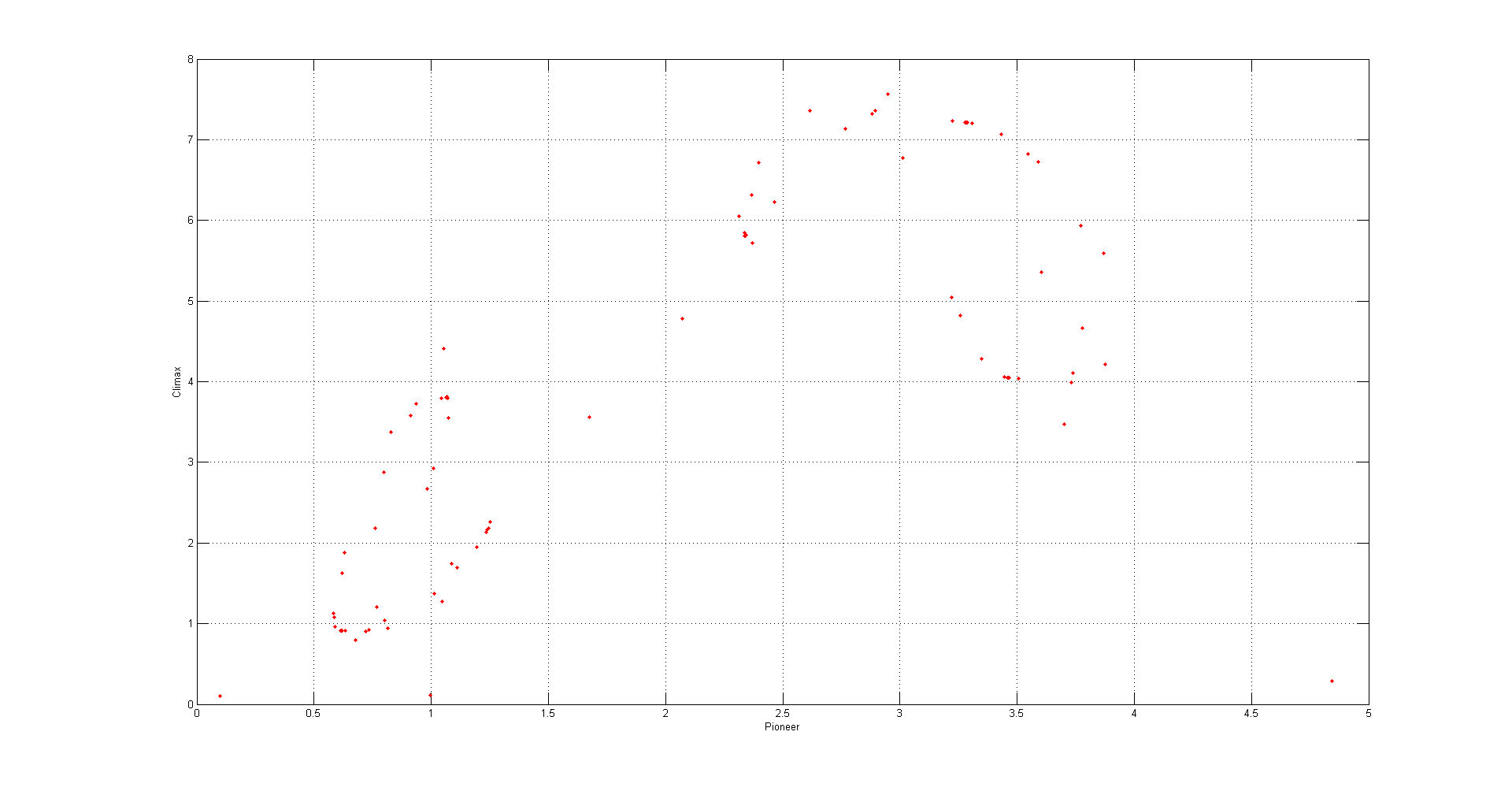
Figure 4: Attractor of transitional multihorseshoe type for the map (11) with $a=2.4,b=2.5$.

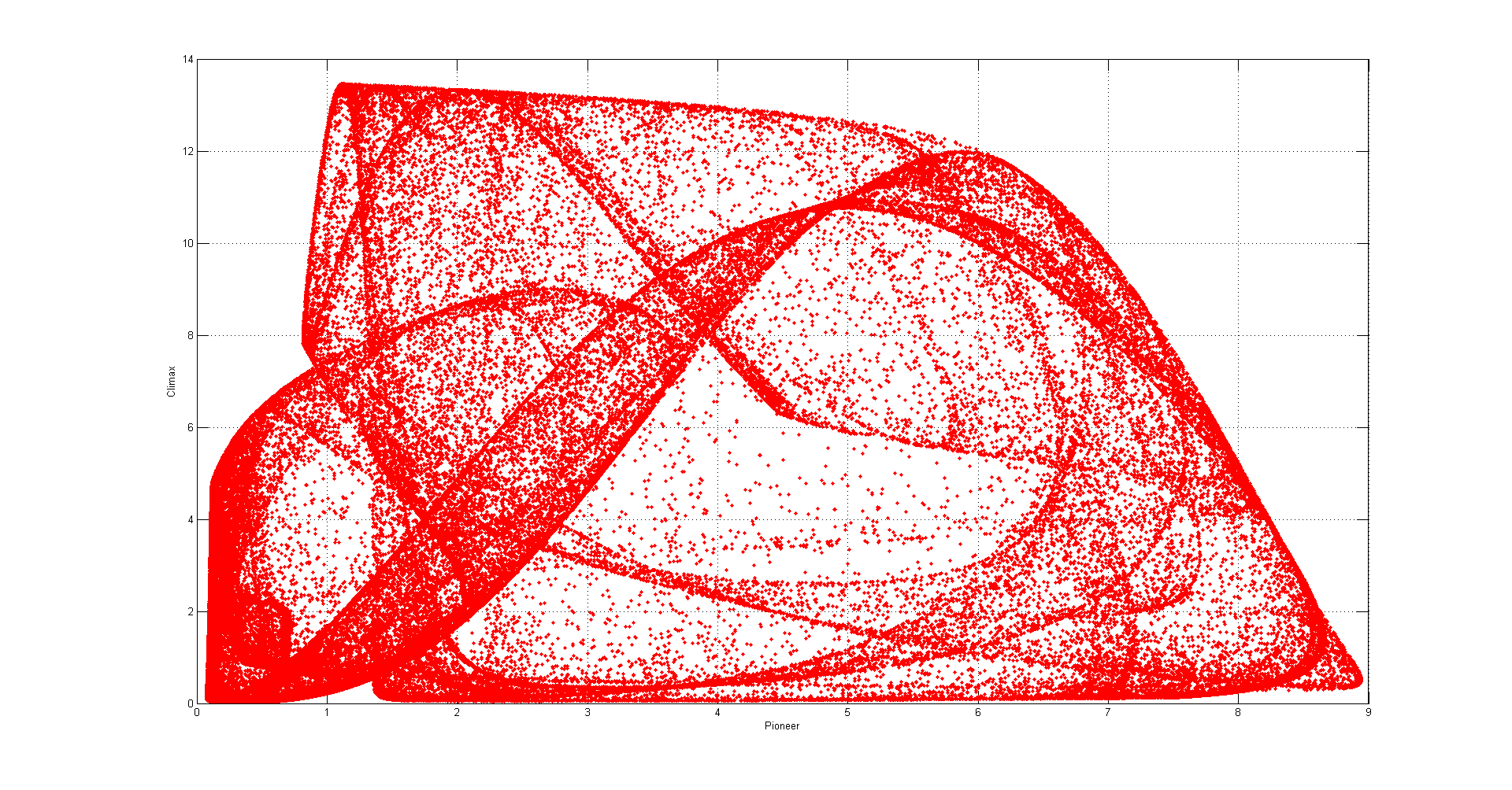
Figure 5: A multihorseshoe chaotic strange attractor for the map (11) with $a=b=3$.

Another example of a multihorseshoe attractor, this time for the map defined as

$$f(x_{1},x_{2})=f(x_{1},x_{2};a,b):=\left(x_{1}e^{a-0.8x_{1}},x_{2}(0.2x_{1}+0.8x_{2})e^{b-0.2x_{1}-0.8x_{2}}\right).$$ (12)

is shown in Fig. 6 for $a=b=3.$

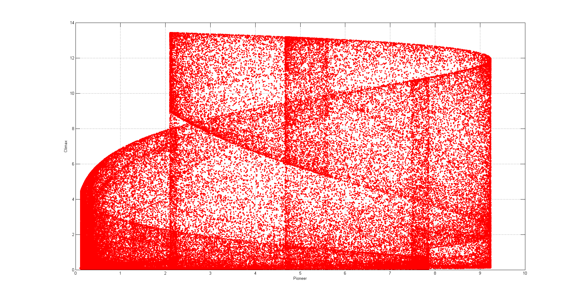
Figure 6: A multihorseshoe chaotic strange attractor for the map (12) with $a=b=3$.

6 Concluding Remarks

We have proved what appear to be several new theorems about strange attractors based on hypotheses that are relatively easy to check, which means that they are rather well suited to a variety of applications amenable to modeling by discrete dynamical systems.

The radial theorems, which apply to asymptotically zero discrete dynamical systems of arbitrary finite dimension, may be viewed as extensions of known results for one-dimensional systems, since it appears that they pretty much coincide with many aspects of much of the work that has appeared in the literature in this case such as that described in [7, 40, 41]. Our multihorseshoe (trellis) results, even though they were at least partially envisaged and analyzed by Easton, can still in large measure be considered as novel inasmuch as they are rigorous extensions of the concepts introduced in [12]. As we also noted, the multihorseshoe attractors are essentially of rank-one type, so it might be interesting to determine how closely our approach is connected with rank-one theory. In addition, an investigation of this connection might lead to some useful new techniques for studying strange attractors that effectively combine elements of both methods.

One of the most attractive features of our multihorseshoe techniques is the possibility they seem to provide for higher dimensional generalizations (with may even extend to infinite-dimensional discrete dynamical systems). In particular, it is natural to enquire if our approach can be used for the construction and identification of chaotic strange attractors generated by unstable manifolds of dimension greater that one. We have already begun to look into this question, and expect to present rigorous versions of our already promising preliminary results in a series of forthcoming papers. In addition to extending and generalizing the results obtained here, we shall continue to seek significant application areas in which our approach or some modifications thereof can be used to answer outstanding questions concerning the existence of strange attractors, which in physical modeling often provide important information about the evolution of a system. For example, recently developed dynamical models of granular flow phenomena such as in [6, 29] appear to have strange attractors that control the long-time behavior of the particle configurations.

References

- [1] D. K. Arrowsmith and C. M. Place, Dynamical Systems: Differential Equations, Maps and Chaotic Behaviour, Chapman and Hall, London, 1992.
- [2] S. Balint, L. Braescu and E. Kaslik, Regions of Attraction and Applications to Control Theory, Cambridge Scientific Publ. Ltd., Cambridge, 2008.
- [3] J. Banks, J. Brooks, G. Cairns, G. Davis and P. Stacey, On Devaney’s definition of chaos, Amer. Math. Monthly 99 (1992), 332-334.
- [4] M. Benedicks and L. Carleson, The dynamics of the Hénon map, Ann. of Math. (2) 133 (1991), 73-169.
- [5] J. Best, C. Castillo-Chavez and A.-A. Yakubu, Hierarchical competition in discrete time models with dispersal, Fields Institute Communications 36 (2004), 59-86.
- [6] D. Blackmore, A. Rosato, X. Tricoche, K. Urban and L. Zuo, Analysis, simulation and visualization of 1D tapping dynamics via reduced dynamical models (submitted).
- [7] H. Bruin, G. Keller, T. Nowicki and S. van Strien, Wild Cantor attractors exist, Ann. of Math. 143 (1996), 97-130.
- [8] B. Cazelles, Dynamics with riddled basins of attraction in models of interacting populations, Chaos, Solitons and Fractals 12 (2001), 301-311.
- [9] L. Chen and K. Aihara, Strange attractors in chaotic neural networks, IEEE Trans. Circuits Syst. 47 (2000), 1455-1468.
- [10] J. Chen, J. and D. Blackmore, On the exponentially self-regulating population model, Chaos, Solitons & Fractals 14 (2002), 1433-1450.
- [11] R. Devaney, An Introduction to Chaotic Dynamics, Addision–Wesley, Boston, 1989.
- [12] R. Easton, Trellises formed by stable and unstable manifolds in the plane, Trans. Amer. Math. Soc. 294 (1986), 719-732.
- [13] K. Falconer, Techniques in Fractal Geometry, Wiley, Chichester, U.K., 1997.
- [14] J. E. Franke and A.-A. Yakubu, Exclusion principle for density-dependent discrete pioneer-climax models, J. Math. Anal. Appl. 187 (1994), 1019-1046.
- [15] J. E. Franke and A.-A. Yakubu, Pioneer exclusion in a one-hump discrete pioneer-climax competitive system, J. Math. Biol. 32 (1994), 771-787.
- [16] C. Grebogi, E. Ott, S. Pelikan and J. Yorke, Strange attractors that are not chaotic, Physica D 13 (1984), 261-268.
- [17] J. Guckenheimer and P. Holmes, Nonlinear Oscillations, Dynamical Systems and Bifurcations of Vector Fields, Springer-Verlag, New York, 1983.
- [18] M. P. Hassell and M. N. Comins, Discrete time models for two-species competition, Theoret. Population Biol. 9 (1976), 202-221.
- [19] A. Hatcher, Algebraic Topology, Cambridge Univ. Press, Cambridge, 2002.
- [20] B. Hunt, J. Kennedy, T-Y. Li and H. Nusse (eds), The Theory of Chaotic Attractors, Springer-Verlag, New York, 2004.
- [21] Y. Joshi, Y. and D. Blackmore, Bifurcation and chaos in higher dimensional pioneer-climax systems, Int’l. Electronic J. Pure and Appl. Math. 1 (3) (2010), 303-337.
- [22] Y. Joshi, Y. and D. Blackmore, Exponentially decaying discrete dynamical systems, Recent Patents on Space Tech. 2 (1) (2012), 37-48.
- [23] F. Marotto, Snap-back repellers imply chaos, J. Math. Anal. Appl. 63 (1978), 199-223.
- [24] J. Milnor, On the concept of attractor, Comm. Math. Phys. 99 (1985), 177-195.
- [25] J. Milnor, Correction and remarks: “On the concept of attractor”, Comm. Math. Phys. 102 (1985), 517-519.
- [26] M. Misiurewicz, Strange attractors for the Lozi mappings, N.Y. Acad. Sci. 357 (1980), 348-358.
- [27] W. Ott and M. Stenslund, From limit cycles to strange attactors, Commun. Math. Phys. 296 (2010), 215-249.
- [28] C. Robinson, Dynamical Systems: Stability, Symbolic Dynamics, and Chaos, CRC Press Inc., Boca Raton, 1995.
- [29] A. Rosato, D. Blackmore, X. Tricoche, K. Urban and L. Zuo, Dynamical systems models and discrete element simulations of a tapped granular column, Powders & Grains 2013, July 8-12, 2013, Sydney, Australia, AIP Conf. Proc. 1541 (2013), pp. 317-320.
- [30] Z. Roupas, Phase space geometry and chaotic attractors in dissipative Nambu mechanics, J. Phys. A: Math.Theor. 45 (2012), 195101.
- [31] D. Ruelle, Chaotic Evolution and Strange Attractors, Lezioni Lincee, Cambridge Univ. Press, Cambridge, 1989.
- [32] W. Schaffer, Order and chaos in ecological systems, Ecology 66 (1985), 93-106.
- [33] W. Schaffer and M. Kot, Do strange attractors govern ecological systems? BioScience 35 (1985), 342-350.
- [34] J. F. Selgrade, Planting and harvesting for pioneer-climax models, Rocky Mountain J. Math. 24 (1994), 293-310.
- [35] J. F. Selgrade and G. Namkoong, Stable periodic behavior in a pioneer-climax model, Nat. Resour. Model 4 (1990), 215-227.
- [36] J. F. Selgrade and J. H. Roberds, On the structure of attractors for discrete, periodically forced systems with applications to population models, Physica D 158 (2001), 69-82.
- [37] J. F. Selgrade and J. H. Roberds, Global attractors for a discrete selection model with periodic immigration, J. Diff. Eqs. and Appl. 15 (2007), 275-287.
- [38] M. Shub, Global Stability of Dynamical Systems, Springer-Verlag, New York, 1987.
- [39] S. Sumner, Hopf bifurcation in pioneer-climax competing species models, Math. Biosci. 137 (1996), 1-24.
- [40] H. Thunberg, Periodicity versus chaos in one-dimensional dynamics, SIAM Review 43 (2001), 3-30.
- [41] J. Ugarcovici and H. Weiss, Chaotic attractors and physical measures for some density dependent Leslie population models, Nonlinearity 20 (2007), 2897-2906.
- [42] Q. Wang and L-S. Young, Strange attractors with one dimension of instability, Commun. Math. Phys. 218 (2001), 1-97.
- [43] Q. Wang and L-S. Young, From invariant curves to strange attractors, Commun. Math. Phys. 225 (2002), 275-304.
- [44] Q. Wang and L-S. Young, Strange attractors in periodically-kicked limit cycles and Hopf bifurcations, Commun. Math. Phys. 240 (2003), 509-529.
- [45] Q. Wang and L-S. Young, Toward a theory of rank one attractors, Ann. of Math. (2) 167 (2008), 349-480.
- [46] S. Wiggins, Introduction to Applied Nonlinear Dynamical Systems and Chaos, Springer, New York, 2003.
- [47] G. Zaslavsky, The simplest case of a strange attractor, Phys. Lett. A 69 (1978/79), 145-147.