Towards a fitting procedure to deeply virtual meson production

– the next-to-leading order case –

D. Müller^a, T. Lautenschlager^b, K. Passek-Kumerički^d, A. Schäfer^b

^aInstitut für Theoretische Physik II, Ruhr-Universität Bochum

D-44780 Bochum, Germany

^b Institut für Theoretische Physik, University Regensburg

D-93040 Regensburg, Germany

^dTheoretical Physics Division, Rudjer Bošković Institute

HR-10002 Zagreb, Croatia

Abstract

Based on the collinear factorization approach, we present a comprehensive perturbative next-to-leading (NLO) analysis of deeply virtual meson production (DVMP). Our representation in conformal Mellin space can serve as basis for a global fitting procedure to access generalized parton distributions from experimental measurements of DVMP and deeply virtual Compton scattering (DVCS). We introduce a rather general formalism for the evaluation of conformal moments that can be developed further beyond the considered order. We also confirm previous diagrammatical findings in the pure singlet quark channel. Finally, we use the analytic properties of the hard scattering amplitudes to estimate qualitatively the size of radiative corrections and illustrate these considerations with some numerical examples. The results suggest that global NLO GPD fits, including both DVMP and DVCS data, could be more stable than often feared.

Keywords: hard exclusive electroproduction, vector mesons, generalized parton distributions

PACS numbers: 11.25.Db, 12.38.Bx, 13.60.Le

1 Introduction

Besides DVCS [1, 2, 3], exclusive electroproduction of mesons in the deeply virtual regime (DVMP), belongs to the class of hard exclusive processes that allows us to access GPDs from experimental measurements [4]. One of the main goals of such fits is to resolve the transverse distribution of partons inside the nucleon [5, 6, 7]. Triggered by the link of GPDs to the partonic spin decomposition of the nucleon [8], GPDs have been intensively studied for some time in theory and a whole framework is now build up around them, see the reviews [9, 10]. The heart of this framework is the phenomenological access to GPDs, based on factorization theorems which ensure that unobservable transverse degrees of freedom can be integrated out if the exchanged photon in DVMP (DVCS) is longitudinally (transversally) polarized. This factorization property of DVMP amplitudes has been shown by diagrammatical considerations for light (pseudo)scalar and longitudinal vector mesons [4]. Thereby, it has been stated that in leading order of $1/{\cal Q}$ the DVMP amplitude factorizes into a hard scattering part and two non-perturbative and process independent distributions. The formation of the meson is described by the corresponding leading twist-two meson distribution amplitude (DA) while the transition from the initial nucleon to the final hadronic state is encoded in twist-two GPDs. Various DVMP channels have been considered to leading order (LO) accuracy of perturbation theory in numerous papers [11, 12, 13, 14, 15, 16, 17, 18]. Knowing that these hard scattering amplitudes are only classified by a flavor non-singlet or singlet label and a signature factor, one can easily extend the processes of phenomenological interest to the level of next-to-leading order (NLO) perturbation theory [19, 20] (for DVCS related processes see[21, 22, 23, 24, 25]). Note that the naive calculation of so-called ‘power-corrections’ [26] is maybe not consistent with the idea that one integrates out transverse degrees of freedom, yielding both perturbative and power-suppressed contributions. Thus, such a simple minded treatment can not be used if one likes to stay with a systematic field theoretical framework. We add that a calculation of kinematical power-corrections to DVMP, as it is feasible in DVCS [27, 28, 29, 30], is a challenging task which has not been studied so far.

Furthermore, much effort has been spend during the last decade to measure the exclusive processes in question in the collider experiments H1 and ZEUS [31, 32, 33, 34, 35, 36, 37], fixed target experiments HERMES [38, 39, 40, 41] and at JLAB [42, 43, 44, 45, 46, 47, 48]. Unfortunately, on the phenomenological side – apart from some earlier model dependent estimates as well as more recent data descriptions for $\pi^{+}$ [49] and light vector mesons [50] at leading order accuracy – the collinear framework has still not been confronted to the increasing amount of experimental DVMP data. However, we like to emphasize here that a GPD inspired hand-bag model approach has been used to link GPD models to DVMP measurements [51, 52, 53]. On the other hand some effort has been spent to analyze DVCS data with flexible GPD models [54, 55, 56], while the idea to describe present DVCS data with some given class of models might be not considered as an appropriate approach [57], see the review [58]. Furthermore, it has been shown that utilizing the model for the dominant $H$ GPD, based on the popular Radyushkin ansatz [59], from the hand-bag approach provides predictions for DVCS on unpolarized protons that reproduce collider DVCS data and are roughly compatible with fixed target DVCS data [60, 50]. Very similar results are obtained if one utilizes the complete GPD content of this model for polarized proton DVCS data [61]. This together with the above mentioned DVMP LO description provides a hint that a global analysis of DVMP and DVCS data might be possible.

In particular in the small-$x_{\rm B}$ region flexible GPD models are needed and used to control both the size and the evolution flow of Compton form factors (CFFs). This was realized when GPDs were directly parameterized in terms of (conformal) Mellin moments [54] rather than in momentum fraction representation. Apart from providing an easy possibility to parameterize GPDs, this technique allows also to set up robust and fast numerics [54, 55]. To apply this technique for a global DVCS and DVMP analysis, the NLO corrections to DVMP are needed, which we will provide in this paper. We will also present explicit formulae for the evaluation of the imaginary part of DVMP amplitudes to NLO accuracy in the momentum fraction representation. Combined with dispersion relation technique, this may offer an alternative possibility for an efficient numerical treatment at least for the purpose to confront some given GPD models in momentum fraction representation with experimental measurements.

In this article we systematize the perturbative framework for DVMP at NLO in such a manner that it can be utilized in a straightforward manner in existing fitting routines for a global analysis of DVCS and DVMP processes. To do so, we will first define transition form factors (TFFs), which allow for a clear separation of observables and the perturbative evaluation procedure on amplitude level. We also complete the set of observables for a DVMP process from two to four. This allow at least in principle for an disentanglement of the imaginary and real parts of TFFs in longitudinal photoproduction if in future the polarization of the final state proton is experimentally measurable, which would provide an additional handle for the access of twist-two GPDs. We also give for the first time a generic discussion of radiative corrections for TFFs and compare them with those of CFFs. The detailed outline of our presentation is as follows.

In Sec. 2 we introduce our nomenclature for TFFs. We parameterize then the longitudinal photon helicity amplitudes in terms of intrinsic parity even and odd TFFs and calculate the longitudinal photon cross section for all possible target polarizations, as well as for the longitudinal polarization of the outgoing nucleon. Furthermore, we perform the charge and flavor decomposition of these TFFs for some important DVMP channels. This allows us in return to present the perturbative corrections in the flavor non-singlet and singlet channel in a compact manner. In Sec. 3 we recall the collinear framework for DVMP in momentum fraction representation, point out the general analytic properties of hard scattering amplitudes, and introduce our conventions. We then explain the evaluation of TFFs from GPDs by means of both the dispersion relation integral and the Mellin–Barnes integral, and shortly discuss mixed representations. Moreover, we develop a method that allows to evaluate the conformal moments by means of a standard Mellin transform. In Sec. 4 we introduce first building blocks for the NLO hard scattering amplitudes in momentum fraction representation, calculate their imaginary parts and their conformal moments. We confirm the result for the pure singlet part at NLO in momentum fraction space [20], present the whole NLO corrections in a more economical manner in this space. From these results we derive compact expressions, so far not listed in the literature, for the imaginary parts of the hard scattering amplitudes and their conformal moments. In Sec. 5 we set up GPD models in Mellin space, discuss the size of radiative NLO corrections from the generic point of view, and provide some numerical examples for the size of radiative corrections. Finally, we give our conclusions and an outlook for the application of this work. Appendix A contains our GPD conventions as well as the conventions for evolution kernels and anomalous dimensions. In App. B we list the expressions for the real part of NLO building blocks and in App. C we discuss some properties of the non-separable building block for the hard scattering amplitude.

2 Preliminaries

Although we are primary interested to use DVMP to access GPDs, we prefer to distinguish clearly between observables and their partonic description, which are conventionally defined w.r.t. a light-cone direction (since momentum is transferred in the $t$-channel in DVMP, one has great liberty to define the light-cone direction in which partons travel). In the following we define first a form factor decomposition of the $\gamma_{L}^{\ast}N\to MN$ amplitude, where for the goal of accessing twist-two GPDs it is sufficient to restrict ourselves to longitudinal polarized photons and scalar components, e.g., longitudinally polarized vector mesons. Note that due to helicity conservation the contributions of transversally polarized mesons connected to quark transversity GPDs vanish to all orders in the strong coupling constant [62, 63, 9]. For the two TFFs of each channel the same nomenclature will be adopted that is used for twist-two GPDs. Hence, one can immediately read off from cross section expressions which information can be accessed in an experiment. To our best knowledge polarization measurements of the recoiled nucleon have not been much discussed with respect to GPD phenomenology, except for $J/\Psi$ electroproduction in [65]. We will fill this gap and show that in a complete measurement, the number of observables matches twice the number of complex valued TFFs. If one can measure these transition form factors, one has the most complete experimental information to access twist-two GPDs. One may, however, employ other frameworks to facilitate their interpretation. Moreover, we will classify the TFFs with respect to parity and $t$-channel charge conjugation parity and decompose them according to $t$-channel flavor flow. Such decomposition can be also used in (GPD) phenomenology as a flavor filter.

TFF ${\mathcal{F}}_{M}^{\text{A}}$	TFF ${\mathcal{F}}_{M}$	in Eq.	(MF,DR,MB)	$\sigma(F^{\text{A}})$
${\mathcal{H}}^{\rm S}_{{\rm V}^{0}_{L}},{\mathcal{E}}^{\rm S}_{{\rm V}^{0}_{L}}$	${\mathcal{H}}_{{\rm V}^{0}_{L}},{\mathcal{E}}_{{\rm V}^{0}_{L}}$	(2.24)	(3.6,3.33,3.64)	$+1$
${\mathcal{H}}^{{{\rm NS}^{(+)}}}_{{\rm V}_{L}},{\mathcal{E}}^{{{\rm NS}^{(+)}}}_{{\rm V}_{L}}$	${\mathcal{H}}_{{\rm V}_{L}},{\mathcal{E}}_{{\rm V}_{L}}$	(2.24,2.26)	(3.1,3.32,3.63)	$+1$
${\mathcal{H}}^{{q^{(-)}}}_{{\rm V}^{\pm}_{L}},{\mathcal{E}}^{{q^{(-)}}}_{{\rm V}^{\pm}_{L}}$	${\mathcal{H}}_{{\rm V}^{\pm}_{L}}$, ${\mathcal{E}}_{{\rm V}^{\pm}_{L}}$	(2.26)	(3.1,3.32,3.63)	$-1$
$\widetilde{\mathcal{H}}^{{q^{(-)}}}_{\rm PS},\widetilde{\mathcal{E}}^{{q^{(-)}}}_{\rm PS}$	$\widetilde{\mathcal{H}}_{{\rm PS}}$, $\widetilde{\mathcal{E}}_{{\rm PS}}$	(2.28,2.29)	(3.1,3.32,3.63)	$+1$
$\widetilde{\mathcal{H}}^{{{\rm NS}^{(+)}}}_{{\rm PS}^{\pm}},\widetilde{\mathcal{E}}^{{{\rm NS}^{(+)}}}_{{\rm PS}^{\pm}}$	$\widetilde{\mathcal{H}}_{{\rm PS}^{\pm}}$, $\widetilde{\mathcal{E}}_{{\rm PS}^{\pm}}$	(2.29)	(3.1,3.32,3.63)	$-1$

Table 1: Nomenclature of flavor dependent TFFs (first column) appearing in the parametrization of the $\gamma_{L}^{\ast}N\to MN$ amplitude for longitudinal vector ($\text{V}_{L}$) and pseudo scalar (PS) mesons $M$ with $J^{PC}$ quantum numbers $1^{--}$ and $0^{-+}$, respectively. The references to the decomposition in which particular TFFs appear are given next. In the third column we refer to formulae which allow to evaluate TFFs from the corresponding GPD $F^{\text{A}}$ in momentum fraction (MF), dispersion relation (DR), and Mellin-Barnes integral (MB) representations, depending on the signature factor $\sigma(F^{\text{A}})$ that is given next. The label $\text{A}\in\{{{\rm NS}^{(+)}},\text{S}\equiv\text{S}^{(+)},{q^{(-)}}\}$ encodes information about flavor decomposition (non-singlet, singlet, quark species) with definite ($t$-channel) charge parity $C=\pm 1$, given by a superscript $(C)$.

In Sec. 2.1 we introduce the aforementioned TFFs, e.g., usable for longitudinal photoproduction of (pseudo)scalar and longitudinal polarized (axial)vector mesons. Furthermore, we calculate the longitudinal photoproduction cross section in terms of these TFFs exactly, including the polarization state of the outgoing nucleon. In Sec. 2.2 we give our conventions for the flavor decomposition of TFFs including their parity and charge conjugation parity assignments. This is exemplified for longitudinal vector and pseudoscalar meson production, which are the phenomenologically most important DVMP processes. The reader, who is only interested in our conventions and defining equations, can find them in Tab. 1, which lists our TFF nomenclature, DVMP processes of interest, and GPD factorization formulae (given in the next section for three different representations). We add that in the twist-two approximation the name of the quark TFFs matches the name of the GPDs.

2.1 Longitudinal photoproduction cross section

Let us first introduce our reference frame for exclusive electroproduction, which is the same as in [66]. The incoming electron momentum has a positive $x$-component, the longitudinal photon with momentum $q_{1}$ travels in the direction of the negative $z$-axis and the nucleon with momentum $p_{1}=(M_{N},0,0,0)$ and polarization vector $s_{1}$, is at rest. The outgoing nucleon has momentum $p_{2}$ and may be polarized along the direction $s_{2}$. Finally, the momentum of the produced meson is called $q_{2}$. The longitudinal polarization vector of the photon can be expressed in terms of the incoming nucleon $p_{1}$ and photon $q_{1}$ momenta

$$\varepsilon_{1}^{\mu}(0) \!\!\!=\!\!\! -\frac{1}{{\cal Q}\sqrt{1+\epsilon^{2}}}\,q_{1}^{\mu}-\frac{2x_{\rm B}}{{\cal Q}\sqrt{1+\epsilon^{2}}}\,p_{1}^{\mu}\,,\quad\epsilon=\frac{2x_{\rm B}M_{N}}{{\cal Q}}\,.$$ (2.1)

We parameterize the photon helicity amplitude for longitudinal photoproduction of a (pseudo)scalar meson $M$ in terms of transition form factors. We are left with four TFFs or, alternatively, nucleon helicity amplitudes, however, by parity conservation these are reduced to two independent ones. We adopt the parametrization for helicity dependent Compton form factors from [67]. By means of the free Dirac equation (Gordon identity) it is easy to see that for the case of even or odd intrinsic parity the form factor basis can be chosen to be:

$$\epsilon_{1}^{\mu}(0)\langle MN|j_{\mu}|N\rangle\!\!\! = \!\!\!\left\{{\overline{u}(p_{2},s_{2})\bigg{[}{\not\!\!m}\,{\mathcal{H}}_{M}+i\sigma_{\alpha\beta}\frac{m^{\alpha}\Delta^{\beta}}{2M_{N}}\,{\mathcal{E}}_{M}\bigg{]}u(p_{1},s_{1})\quad\mbox{parity even}\atop\overline{u}(p_{2},s_{2})\bigg{[}{\not\!\!m}\gamma_{5}\,\widetilde{\mathcal{H}}_{M}+\gamma_{5}\frac{m\cdot\Delta}{2M_{N}}\,\widetilde{\mathcal{E}}_{M}\bigg{]}u(p_{1},s_{1})\quad\mbox{parity odd}}\right.,$$ (2.2)

where $\Delta^{\mu}=p_{2}^{\mu}-p_{1}^{\mu}=q_{1}^{\mu}-q_{2}^{\mu}$ is the momentum transfer in the $t$-channel ($t\equiv\Delta^{2}$). The choice of the vector $m^{\mu}$ is not unique. To stay close to the conventions, used by us for DVCS, as well as to have a $s\leftrightarrow u$ symmetric energy variable, a favored choice for dispersion relation analysis, we choose the following vector [67]

$$m^{\mu}=\frac{q^{\mu}}{P\cdot q},\quad\mbox{where}\quad q^{\mu}=\frac{1}{2}\left(q_{1}^{\mu}+q_{2}^{\mu}\right)\,,\quad P^{\mu}=p_{1}^{\mu}+p_{2}^{\mu}\,.$$ (2.3)

The photoproduction cross sections in terms of these TFFs (2.2) is straightforwardly calculated. In fact, if the meson mass is neglected, the formulae for an unpolarized outgoing nucleon can be read off from the expressions for DVCS [67]. For the conversion of electroproduction to photoproduction cross section we adopt the Hand convention [68], which fixes the photon flux and yields

$$\frac{d\sigma^{\gamma_{\rm L}^{*}\,N\to M\,N}}{dtd\varphi} \!\!\!= \!\!\!\frac{2\pi\alpha_{\rm em}}{{\cal Q}^{4}\sqrt{1+\epsilon^{2}}}\,\frac{x_{\rm B}^{2}}{1-x_{\rm B}}\frac{1}{2}\Big{\{}{\cal C}_{\rm unp}({\mathcal{F}}_{M},{\mathcal{F}}_{M}^{\ast}|s_{2})+\Lambda\cos(\theta){\cal C}_{\rm LP}({\mathcal{F}}_{M},{\mathcal{F}}_{M}^{\ast}|s_{2})$$

$$\phantom{\frac{2\pi\alpha_{\rm em}}{{\cal Q}^{4}}}+\Lambda\cos(\varphi)\sin(\theta)\,{\cal C}_{{\rm TP}+}({\mathcal{F}}_{M},{\mathcal{F}}_{M}^{\ast}|s_{2})+\Lambda\sin(\varphi)\sin(\theta)\,{\cal C}_{{\rm TP}-}({\mathcal{F}}_{M},{\mathcal{F}}_{M}^{\ast}|s_{2})\Big{\}}\,.$$

Here, $\alpha_{\rm em}\approx 1/137$ is the electromagnetic fine structure constant, $q_{1}^{2}=-{\cal Q}^{2}$ is the photon virtuality, $x_{\rm B}={\cal Q}^{2}/p_{1}\cdot q_{1}$ is the Bjorken variable and $\varphi=\Phi-\phi$, where $\Phi$ appears in the transverse part of the polarization vector

$$s_{1}=(0,\cos\Phi\cos\theta,\sin\Phi\cos\theta,\sin\theta)$$

and $\phi$ is the azimuthal angle between the electron plane and the recoiled proton. Furthermore, the squared scattering amplitudes $\cal C$ are labeled by the polarization of the incoming nucleon. Note that when summed over the final state proton polarization, the conventional factor $1/2$ on the r.h.s. will disappear.

The bilinear $\cal C$-coefficients depend on the polarization direction of the outgoing nucleon, which provides the possibility to measure various combinations of TFFs. In experiments where the outgoing protons are unpolarized one can only access the cross section for a transversally polarized nucleon, which contains for scalar or longitudinally polarized vector meson production the terms

$${\cal C}_{\rm unp}({\mathcal{F}},{\mathcal{F}}^{\ast}) \!\!\!=\!\!\! \frac{4(1-x_{\rm B})\left(1-x_{\rm B}\frac{m^{2}-t}{{\cal Q}^{2}}\right)-\frac{m^{2}}{M^{2}}\epsilon^{2}}{\left(2-x_{\rm B}-x_{\rm B}\frac{m^{2}-t}{{\cal Q}^{2}}\right)^{2}}\Bigg{|}{\mathcal{H}}-\frac{x_{\rm B}^{2}\left(1+\frac{m^{2}-t}{{\cal Q}^{2}}\right)^{2}+4x_{\rm B}^{2}\frac{t}{{\cal Q}^{2}}}{4(1-x_{\rm B})\left(1-x_{\rm B}\frac{m^{2}-t}{{\cal Q}^{2}}\right)-\frac{m^{2}}{M^{2}}\epsilon^{2}}{\mathcal{E}}\Bigg{|}^{2}$$ (2.5)

$$+\frac{1}{(1-x_{\rm B})\left(1-x_{\rm B}\frac{m^{2}-t}{{\cal Q}^{2}}\right)-\frac{m^{2}}{4M^{2}}\epsilon^{2}}\,\frac{\widetilde{K}^{2}}{4M^{2}}\left|{\mathcal{E}}\right|^{2}\,,$$

$${\cal C}_{{\rm TP}-}({\mathcal{F}},{\mathcal{F}}^{\ast}) \!\!\!=\!\!\! -\frac{2}{2-x_{\rm B}-x_{\rm B}\frac{m^{2}-t}{{\cal Q}^{2}}}\,\frac{\widetilde{K}}{M}\Im{\rm m}{\mathcal{H}}{\mathcal{E}}^{\ast}\,,$$ (2.6)

and for pseudo scalar or longitudinal polarized axial-vector meson production the terms

$$\widetilde{\cal C}_{\rm unp}({\mathcal{F}},{\mathcal{F}}^{\ast}) \!\!\!=\!\!\! \frac{4(1-x_{\rm B})\left(1-x_{\rm B}\frac{m^{2}-t}{{\cal Q}^{2}}\right)+\epsilon^{2}\left(2-\frac{m^{2}}{M^{2}}-\frac{2m^{2}-t}{{\cal Q}^{2}}\right)}{\left(2-x_{\rm B}-x_{\rm B}\frac{m^{2}-t}{{\cal Q}^{2}}\right)^{2}}$$

$$\times\Bigg{|}\widetilde{\mathcal{H}}-\frac{x_{\rm B}\left(1+\frac{m^{2}}{{\cal Q}^{2}}\right)^{2}\left(2-x_{\rm B}-x_{\rm B}\frac{m^{2}-t}{{\cal Q}^{2}}\right)}{4(1-x_{\rm B})\left(1-x_{\rm B}\frac{m^{2}-t}{{\cal Q}^{2}}\right)+\epsilon^{2}\left(2-\frac{m^{2}}{M^{2}}-\frac{2m^{2}-t}{{\cal Q}^{2}}\right)}\overline{\mathcal{E}}\Bigg{|}^{2}$$

$$+\frac{4\left(1+\frac{m^{2}}{{\cal Q}^{2}}\right)^{2}}{4(1-x_{\rm B})\left(1-x_{\rm B}\frac{m^{2}-t}{{\cal Q}^{2}}\right)+\epsilon^{2}\left(2-\frac{m^{2}}{M^{2}}-\frac{2m^{2}-t}{{\cal Q}^{2}}\right)}\,\frac{\widetilde{K}^{2}}{4M^{2}}\left|\overline{\mathcal{E}}\right|^{2}\,,$$

$$\widetilde{\cal C}_{{\rm TP}-}({\mathcal{F}},{\mathcal{F}}^{\ast}) \!\!\!=\!\!\! \frac{2\left(1+\frac{m^{2}}{{\cal Q}^{2}}\right)}{2-x_{\rm B}-x_{\rm B}\frac{m^{2}-t}{{\cal Q}^{2}}}\,\frac{\widetilde{K}}{M}\Im{\rm m}\widetilde{\mathcal{H}}\overline{\mathcal{E}}^{\ast}\,.$$ (2.8)

Here, the kinematical factor

$$\widetilde{K}=\sqrt{-M^{2}x_{\rm B}^{2}\left[\!\left(1-\frac{m^{2}-t}{{\cal Q}^{2}}\right)^{2}+\frac{4m^{2}}{{\cal Q}^{2}}\left(1-\frac{t}{4M^{2}}\right)\!\right]-(1-x_{\rm B})t\left(1-x_{\rm B}\frac{m^{2}-t}{{\cal Q}^{2}}\right)}$$ (2.9)

vanishes at the minimal and maximal allowed value of $-t$,

$$t_{\rm min/max}=-{\cal Q}^{2}\frac{2\left(1-x_{\rm B}-x_{\rm B}\frac{m^{2}}{{\cal Q}^{2}}\right)+\epsilon^{2}\left(1-\frac{m^{2}}{{\cal Q}^{2}}\right)\mp 2\sqrt{1+\epsilon^{2}}\sqrt{\left(1-x_{\rm B}-x_{\rm B}\frac{m^{2}}{{\cal Q}^{2}}\right)^{2}-\frac{m^{2}}{{\cal Q}^{2}}\epsilon^{2}}}{4(1-x_{\rm B})x_{\rm B}+\epsilon^{2}},\quad$$ (2.10)

where the lower and upper sign applies for $t_{\rm min}$ and $t_{\rm max}$, respectively. The unpolarized ${\cal C}$-coefficients (2.5,2.1) are build from two squared terms while the square of target spin flip TFFs is naturally accompanied by a $\widetilde{K}^{2}/4M^{2}$ suppression factor. Relying on this kinematical suppression, one can essentially extract from unpolarized cross section measurements at smaller values of $x_{\rm B}$ the modulus of the TFFs ${\mathcal{H}}$ or $\widetilde{\mathcal{H}}$. Having a transversally polarized proton at hand, the single target spin asymmetry offers an access to the combinations (2.6) and (2.8), see, e.g., phenomenologically discussions in [69, 53, 49]. Note that the quantity $\overline{\cal E}=x_{\rm B}\,\widetilde{\mathcal{E}}/(2-x_{\rm B}-x_{\rm B}\frac{m^{2}-t}{{\cal Q}^{2}})$ absorbs one additional power of $x_{\rm B}$, and thus has the same Regge counting as the other TFFs.

In experiments where the polarization of the outgoing proton can be measured, one can access further TFF combinations. However, it turns out that the transverse-to-transverse proton spin contribution does not contain new information rather it offers access to the unpolarized TFF combinations (2.5,2.1), while the final state transverse single spin asymmetry provides again the imaginary parts (2.6) and (2.8). The remaining terms will project on the longitudinal component of the final state polarization vector. Hence, choosing the longitudinal magnetization direction

$$s^{\parallel}_{2}=\frac{1}{\sqrt{\left(p_{2}^{0}\right)^{2}-\left(p_{2}^{3}\right)^{2}}}\left(p_{2}^{3},0,0,p_{2}^{0}\right)$$

provides the most appropriate handle to access two new TFF combinations. We find the following combinations

$${\cal C}_{{\rm LP}}({\mathcal{F}},{\mathcal{F}}^{\ast}|s_{2}^{\parallel}) \!\!\!=\!\!\! \frac{\sqrt{1+\epsilon^{2}}}{\sqrt{1+\epsilon^{2}+\frac{\widetilde{K}^{2}}{M^{2}}}}\Bigg{\{}{\cal C}_{\rm unp}({\mathcal{F}},{\mathcal{F}}^{\ast})-\frac{2\widetilde{K}^{2}}{M^{2}\left(2-x_{\rm B}-x_{\rm B}\frac{m^{2}-t}{{\cal Q}^{2}}\right)^{2}}$$

$$\phantom{\frac{\sqrt{1+\epsilon^{2}}}{\sqrt{1+\epsilon^{2}+\frac{\widetilde{K}^{2}}{M^{2}}}}}\times\Bigg{(}\left|{\mathcal{H}}+{\mathcal{E}}\right|^{2}-\frac{1}{1+\epsilon^{2}}\left|{\mathcal{H}}+\frac{x_{\rm B}}{2}\Big{(}1+\frac{m^{2}-t}{{\cal Q}^{2}}\Big{)}{\mathcal{E}}\right|^{2}\Bigg{)}\Bigg{\}},$$

$${\cal C}_{{\rm TP}+}({\mathcal{F}},{\mathcal{F}}^{\ast}|s_{2}^{\parallel}) \!\!\!=\!\!\! \frac{-\widetilde{K}}{M\sqrt{1+\epsilon^{2}}\sqrt{1+\epsilon^{2}+\frac{\widetilde{K}^{2}}{M^{2}}}}\Bigg{\{}{\cal C}_{\rm unp}({\mathcal{F}},{\mathcal{F}}^{\ast})+\frac{2\epsilon^{2}}{2-x_{\rm B}-x_{\rm B}\frac{m^{2}-t}{{\cal Q}^{2}}}\Big{|}{\mathcal{H}}+\frac{t}{4M^{2}}{\mathcal{E}}\Big{|}^{2}$$ (2.12)

$$+\frac{2(1+\epsilon^{2})}{2-x_{\rm B}-x_{\rm B}\frac{m^{2}-t}{{\cal Q}^{2}}}\,\Re{\rm e}{\mathcal{H}}{\mathcal{E}}^{\ast}-\frac{\widetilde{K}^{2}-t\left(1+\epsilon^{2}\right)}{2M^{2}\left(2-x_{\rm B}-x_{\rm B}\frac{m^{2}-t}{{\cal Q}^{2}}\right)}\left|{\mathcal{E}}\right|^{2}\Bigg{\}},$$

for longitudinally polarized vector or scalar meson production and

$$\widetilde{\cal C}_{{\rm LP}}({\mathcal{F}},{\mathcal{F}}^{\ast}|s_{2}^{\parallel}) \!\!\!=\!\!\! \frac{\sqrt{1+\epsilon^{2}}}{\sqrt{1+\epsilon^{2}+\frac{\widetilde{K}^{2}}{M^{2}}}}\Bigg{\{}\widetilde{\cal C}_{\rm unp}({\mathcal{F}},{\mathcal{F}}^{\ast})-\frac{8x_{\rm B}\widetilde{K}^{2}}{{\cal Q}^{2}\left(1+\epsilon^{2}\right)}\frac{1-x_{\rm B}+x_{\rm B}\frac{M^{2}}{{\cal Q}^{2}}}{\left(2-x_{\rm B}-x_{\rm B}\frac{m^{2}-t}{{\cal Q}^{2}}\right)^{2}}\left|\widetilde{\mathcal{H}}\right|^{2}\qquad$$

$$-\frac{2\left(1+\frac{m^{2}}{{\cal Q}^{2}}\right)\left(1+x_{\rm B}\frac{2M^{2}}{{\cal Q}^{2}}\right)}{\left(1+\epsilon^{2}\right)\left(2-x_{\rm B}-x_{\rm B}\frac{m^{2}-t}{{\cal Q}^{2}}\right)}\frac{\widetilde{K}^{2}}{M^{2}}\Re{\rm e}\widetilde{\mathcal{H}}\overline{\mathcal{E}}^{\ast}-\frac{\left(1+\frac{m^{2}}{{\cal Q}^{2}}\right)^{2}}{1+\epsilon^{2}}\frac{\widetilde{K}^{2}}{2M^{2}}\left|\overline{\mathcal{E}}\right|^{2}\Bigg{\}},$$

$$\widetilde{\cal C}_{{\rm TP}+}({\mathcal{F}},{\mathcal{F}}^{\ast}|s_{2}^{\parallel}) \!\!\!=\!\!\! \frac{\widetilde{K}}{M\sqrt{1+\epsilon^{2}}\sqrt{1+\epsilon^{2}+\frac{\widetilde{K}^{2}}{M^{2}}}}\Bigg{\{}\!\left(\!1+\frac{2x_{\rm B}M^{2}}{{\cal Q}^{2}}\!\right)\widetilde{\cal C}_{\rm unp}({\mathcal{F}},{\mathcal{F}}^{\ast})$$

$$+\frac{2\epsilon^{2}\left(1+\frac{m^{2}}{{\cal Q}^{2}}\right)\left(1-x_{\rm B}+\frac{x_{\rm B}M^{2}}{{\cal Q}^{2}}\right)}{\left(2-x_{\rm B}-x_{\rm B}\frac{\left(m^{2}-t\right)}{{\cal Q}^{2}}\right)^{2}}\Big{|}\widetilde{{\mathcal{H}}}\Big{|}^{2}+\frac{2+\frac{4(1-x_{\rm B})x_{\rm B}t}{{\cal Q}^{2}}+\left(2+\frac{t}{{\cal Q}^{2}}\right)\epsilon^{2}}{2-x_{\rm B}-x_{\rm B}\frac{m^{2}-t}{{\cal Q}^{2}}}$$

$$\times\left(1+\frac{m^{2}}{{\cal Q}^{2}}\right)\Re{\rm e}\widetilde{\mathcal{H}}\overline{\mathcal{E}}^{\ast}+\frac{\left(1+\frac{m^{2}}{{\cal Q}^{2}}\right)^{2}\left(t-x_{\rm B}M^{2}\left(1+\frac{m^{2}-2t}{{\cal Q}^{2}}\right)\right)}{2M^{2}}\left|\overline{\mathcal{E}}\right|^{2}\Bigg{\}},$$

for longitudinally polarized axial-vector or pseudoscalar meson production.

In particular in the smaller-$x_{\rm B}$ region we have the following combinations, e.g., for longitudinally polarized vector meson production

$${\cal C}_{\rm unp}({\mathcal{F}},{\mathcal{F}}^{\ast}) \!\!\!\simeq\!\!\! |{\mathcal{H}}|^{2}-\frac{t}{4M^{2}}|{\mathcal{E}}|^{2}\,,\quad\;\;{\cal C}_{\rm LP}({\mathcal{F}},{\mathcal{F}}^{\ast}|s_{2}^{\parallel})\simeq\sqrt{1-\frac{t}{M^{2}}}\left[|{\mathcal{H}}|^{2}+\frac{t\,|2{\mathcal{H}}+{\mathcal{E}}|^{2}}{4\left(M^{2}-t\right)}\right],$$ (2.15)

$${\cal C}_{{\rm TP}-}({\mathcal{F}},{\mathcal{F}}^{\ast}) \!\!\!\simeq\!\!\! -\frac{\sqrt{-t}}{M}\Im{\rm m}{\mathcal{H}}{\mathcal{E}}^{\ast}\,,\qquad{\cal C}_{{\rm TP}+}({\mathcal{F}},{\mathcal{F}}^{\ast}|s_{2}^{\parallel})\simeq\frac{\sqrt{-t}\sqrt{1-\frac{t}{M^{2}}}}{4M}\left[|{\mathcal{E}}|^{2}-\frac{|2{\mathcal{H}}+{\mathcal{E}}|^{2}}{1-\frac{t}{M^{2}}}\right].$$

An analog formula set is also valid for pseudo scalar meson production, obtained by substituting

$${\mathcal{H}}\to\widetilde{\mathcal{H}}\,,\quad{\mathcal{E}}\to(1+m^{2}/{\cal Q}^{2})\overline{\mathcal{E}}\,,\quad\mbox{and}\quad{\cal C}_{{\rm TP}\pm}\to-\widetilde{\cal C}_{{\rm TP}\pm}\,.$$

Since in the ${\cal C}_{{\rm TP}+}$ expression both kinds of TFFs enter on the same kinematical level, one clearly realizes that transverse-to-longitudinal target spin flip measurements yield a handle on ${\mathcal{E}}$ (and $\overline{\mathcal{E}}$) for $-t\gg 0$. One the other hand, longitudinal-to-longitudinal spin flip cross sections are expected to be dominated for $-t\ll 4M^{2}$ by the modulus $|{\mathcal{H}}|$. However, since $\overline{\mathcal{E}}$ may contain a pion pole contribution, e.g., in $\pi^{+}$ production, the $t/4M^{2}$ suppression factor can be overcompensated. Hence, such a measurement would be helpful for a complete disentanglement of parity odd TFFs, where of course one should bear in mind that in contrast to ${\mathcal{E}}$ the TFF $\overline{\mathcal{E}}$ does not contain a ‘pomeron’ exchange.

2.2 Flavor decomposition of transition form factors

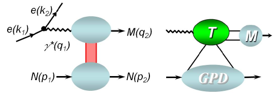
Figure 1: DVMP process from the $t$-channel view (left) and partonic view (right).

To perform a flavor decomposition of the TFFs (2.2) we rely on the quark picture and consider the processes of interest from the $t$-channel point of view as an exchange of colorless degrees of freedom that can be associated with a quark-antiquark or gluon pair, see Fig. 1. We note that $t$-channel contributions are the dominant ones for both large ${\cal Q}^{2}$, i.e., when partonic $t$-channel exchanges are justified by (diagrammatical) power counting, and high-energy limit, e.g., in Regge phenomenology where mesonic degrees of freedom are utilized. Based on the $t$-channel exchange of quark-antiquark pairs we start by performing a flavor decomposition of the TFFs (2.2). This more general classification scheme matches with the nomenclature in the partonic description of DVMP amplitudes in terms of twist-two GPDs and meson DAs.

First, however, we introduce discrete $t$-channel quantum numbers which are used to label GPDs and TFFs. It is instructive to see that from a partonic point of view in the $t$-channel reaction $\gamma^{\ast}q\bar{q}(gg)\to M^{0}$ in which the photon scatters on a $q\bar{q}$ ($gg$) pair, picked up from the proton and described by GPD, and then forms a meson. Note that corresponding crossed processes where analyzed on similar basis in [70, 71] and [72]. From $C_{\gamma}=-1$ and charge parity conservation follows that the $q\overline{q}$ ($gg$) state has to satisfy

$$C=C_{\gamma}C_{M^{0}}=-C_{M^{0}}$$ (2.16)

or, in other words, that the $t$-channel charge parity is given by $(-C_{M^{0}})$. The charge parity of the meson can be read off from the $J^{PC}$ nomenclature with angular momentum $J$, parity $P$, and charge parity $C$, and for vector (${\text{V}}^{0}$) mesons of interest is $1^{--}$ while for pseudoscalar ($\text{PS}^{0}$) mesons $0^{-+}$. Due to the fact that $C_{gg}=1$ it follows trivially that there is no $gg$ contribution for $\text{PS}^{0}$ production (as well as, there are no $gg$ Fock states in ${\text{V}}^{0}$ mesons). Furthermore, since $P_{\gamma}=-1$, the $CP$ quantum number is given by $CP=C_{M^{0}}P_{M^{0}}$ and it corresponds to intrinsic GPD parity or, to say it in (2.2) nomenclature, the production of vector mesons is described by TFFs ${\mathcal{F}}\in\{{\mathcal{H}},{\mathcal{E}}\}$ with even intrinsic parity, while the production of pseudoscalar mesons is described by odd intrinsic parity TFFs ${\mathcal{F}}\in\{\widetilde{\mathcal{H}},\widetilde{\mathcal{E}}\}$. The TFFs derived by using GPDs with well defined charge parity will then be denoted by ${\mathcal{F}}^{(C)}$.

Next we define the flavor content of the considered final meson state in terms of quark-antiquark degrees of freedom. Normalizing all states to one, we expand the charged meson states in terms of the leading quark-antiquark Fock states

$$|M^{0}\rangle=\sum_{q}c_{M^{0}}^{q}\,|q\overline{q}\rangle\quad\mbox{and}\quad|M^{\pm}\rangle=\sum_{q\overline{q}^{\prime}}c_{M^{\pm}}^{q\overline{q}^{\prime}}\,|q\overline{q}^{\prime}\rangle\,,$$ (2.17)

respectively. For neutral mesons the Clebsch-Gordon coefficients are flavor diagonal, while they are flavor off-diagonal for charged meson. The interaction of the longitudinal photon with a quark or an antiquark gives us then a fractional quark charge factor

$$e_{q}\in\left\{e_{u}=\frac{2}{3},e_{d}=-\frac{1}{3},e_{c}=\frac{2}{3},e_{s}=-\frac{1}{3},\cdots\right\}\,,$$ (2.18)

which is together with the Clebsch-Gordon coefficients factorized out. This defines us the quark decomposition of TFFs

$${\mathcal{F}}_{M^{0}}=\sum_{q}e_{q}\,c_{M^{0}}^{q}\,{\mathcal{F}}_{M^{0}}^{q}\quad\mbox{and}\quad{\mathcal{F}}_{M^{\pm}}=e_{q}\,{\mathcal{F}}_{M^{\pm}}^{q\overline{q}^{\prime}}+e_{q^{\prime}}\,{\mathcal{F}}_{M^{\pm}}^{q^{\prime}\overline{q}}\,.$$ (2.19a)

Assuming that isospin symmetry holds true, we may express the flavor off-diagonal nucleon TFFs in terms of flavor diagonal TFFs ones, see, e.g., [15], yielding

$${\mathcal{F}}_{M^{\pm}}=\frac{e_{q}-e_{q^{\prime}}}{2}\left[{\mathcal{F}}_{M^{0}}^{q^{(-C)}}-{\mathcal{F}}_{M^{0}}^{q^{\prime(-C)}}\right]+\frac{e_{q}+e_{q^{\prime}}}{2}\left[{\mathcal{F}}_{M^{0}}^{q^{(C)}}-{\mathcal{F}}_{M^{0}}^{q^{\prime(C)}}\right].$$ (2.19b)

The information about $t$-channel charge parity is encoded in the quark superscript, e.g., ${\mathcal{H}}^{{u^{(+)}}}$ (${\mathcal{E}}^{{u^{(+)}}}$) stands for a $t$-channel exchange of a $u\overline{u}$ pair with even charge parity and even intrinsic parity, where loosely spoken proton helicity is (non)conserved.

Finally, in the charge even sector also gluons can be exchanged in the $t$-channel which may have a flavor quark singlet admixture. Such a contribution will be denoted as ${\mathcal{F}}^{\text{G}}+{\mathcal{F}}^{\mathrm{pS}}$, where subscript ${\mathrm{pS}}$ stands for a pure singlet quark. To separate quark degrees and gluonic ones in the most clean manner it is necessary to change from a quark/gluon basis to group theoretical irreducible SU($n_{f}$) multiplets, consisting out of the flavor non-singlet (NS) multiplets (${\mathcal{F}}^{3}$, $\ldots$, ${\mathcal{F}}^{n_{f}^{2}-1}$) and the flavor singlet one (${\mathcal{F}}^{0}$). Such decomposition solves also the quark-gluon mixing problem that appears in the perturbatively predicted evolution. For $n_{f}=3$ ($n_{f}=4$) this group theoretical decomposition follows from the multiplets (A.9) and reads

$${\mathcal{F}}^{u^{(+)}} \!\!\!= \!\!\!\frac{1}{2}{\mathcal{F}}^{3^{(+)}}+\frac{1}{6}{\mathcal{F}}^{8^{(+)}}+\frac{1}{3}{\mathcal{F}}^{0^{(+)}}+\frac{1}{12}\left({\mathcal{F}}^{15^{(+)}}-{\mathcal{F}}^{0^{(+)}}\right),$$ (2.20a)

$${\mathcal{F}}^{d^{(+)}} \!\!\!= \!\!\!-\frac{1}{2}{\mathcal{F}}^{3^{(+)}}+\frac{1}{6}{\mathcal{F}}^{8^{(+)}}+\frac{1}{3}{\mathcal{F}}^{0^{(+)}}+\frac{1}{12}\left({\mathcal{F}}^{15^{(+)}}-{\mathcal{F}}^{0^{(+)}}\right),$$ (2.20b)

$${\mathcal{F}}^{s^{(+)}} \!\!\!= \!\!\!-\frac{1}{3}{\mathcal{F}}^{8^{(+)}}+\frac{1}{3}{\mathcal{F}}^{0^{(+)}}+\frac{1}{12}\left({\mathcal{F}}^{15^{(+)}}-{\mathcal{F}}^{0^{(+)}}\right),$$ (2.20c)

$${\mathcal{F}}^{c^{(+)}} \!\!\!= \!\!\!-\frac{1}{4}\left({\mathcal{F}}^{15^{(+)}}-{\mathcal{F}}^{0^{(+)}}\right).$$ (2.20d)

Obviously, for $n_{f}=4$ this decomposition reduces smoothly for ${\mathcal{F}}^{c^{(+)}}=0$, i.e., ${\mathcal{F}}^{15^{(+)}}={\mathcal{F}}^{0^{(+)}}$ to the well known SU(3) one. We add that one may perform also such decomposition in the charge odd sector, however, this is not a necessity, since a gluon pair has charge parity even and so no quark-gluon mixing problem appears.

In the following the flavor decomposition of the longitudinal photoproduction TFFs is listed for the phenomenologically most important processes as they appear in the exclusive light meson electroproduction off proton. Namely, of vector mesons extensively measured in both collider and fixed target kinematics at H1 [31, 32, 33], ZEUS [34, 35, 36, 37], HERMES [38, 39], E665 [73], NMC [74], COMPASS [75], CLAS [42, 43, 44, 45], and CORNELL [76] as well as pseudoscalar mesons in fixed target kinematics at HERMES [40, 41], CLAS [46, 47], and HALL-C [48].

• DV$\!V_{L}$P: longitudinal vector meson TFFs ${\mathcal{H}}_{{\rm V}_{L}}^{\text{A}}$ and ${\mathcal{E}}_{{\rm V}_{L}}^{\text{A}}$ for $\gamma_{L}^{\ast}\,p\to V_{L}^{0}\,p$ and $\gamma_{L}^{\ast}\,p\to V_{L}^{+}\,n$.

For longitudinal vector meson (V$=1^{--}$) photoproduction the TFFs are ${\mathcal{H}}_{\rm V},{\mathcal{E}}_{\rm V}$ and for neutral ones we have definite $t$-channel charge parity $C=+1$, see (2.16). The light neutral vector mesons have according to the (constituent) quark model the Fock state expansion

$$|\rho^{0}\rangle=\frac{1}{\sqrt{2}}\left(|u\overline{u}\,\rangle-|d\bar{d}\rangle\right)\,,\quad|\omega\rangle=\frac{1}{\sqrt{2}}\left(|u\overline{u}\,\rangle+|d\bar{d}\rangle\right)\,,\quad|\phi\rangle=|s\bar{s}\rangle\,.$$ (2.21)

As already noted, a two gluon component, which has charge parity even, can not appear in these meson states. We decompose the TFFs ${\mathcal{F}}\in\{{\mathcal{H}},{\mathcal{E}}\}$ with respect to quark and gluonic $t$-channel exchanges according to (2.19a),

$${\mathcal{F}}_{\rho^{0}} \!\!\!=\!\!\! \frac{2}{3\sqrt{2}}{\mathcal{F}}_{\rho^{0}}^{{u^{(+)}}}+\frac{1}{3\sqrt{2}}{\mathcal{F}}_{\rho^{0}}^{{d^{(+)}}}+\frac{1}{\sqrt{2}}\,\left({\mathcal{F}}_{\rho^{0}}^{{\text{G}}}+{\mathcal{F}}_{\rho^{0}}^{{\mathrm{pS}}}\right)\,,$$ (2.22a)

$${\mathcal{F}}_{\omega} \!\!\!=\!\!\! \frac{2}{3\sqrt{2}}{\mathcal{F}}^{{u^{(+)}}}_{\omega}-\frac{1}{3\sqrt{2}}{\mathcal{F}}^{{d^{(+)}}}_{\omega}+\frac{1}{3\sqrt{2}}\,\left({\mathcal{F}}^{{\text{G}}}_{\omega}+{\mathcal{F}}^{{\mathrm{pS}}}_{\omega}\right)\,,$$ (2.22b)

$${\mathcal{F}}_{\phi} \!\!\!=\!\!\! -\frac{1}{3}{\mathcal{F}}^{{s^{(+)}}}_{\phi}-\frac{1}{3}\,\left({\mathcal{F}}^{{\text{G}}}_{\phi}+{\mathcal{F}}^{{\mathrm{pS}}}_{\phi}\right)\,.$$ (2.22c)

Since the $t$-channel exchanges of two gluons or pure singlet quark-antiquark pairs is flavor blind, the factors in front of $\left({\mathcal{F}}^{{\text{G}}}_{{\rm V}^{0}}+{\mathcal{F}}^{{\mathrm{pS}}}_{{\rm V}^{0}}\right)$ are simply given as the sum over all quark coefficients in the corresponding formulae (2.22). Here, the quark TFFs ${\mathcal{F}}^{{q^{(+)}}}_{{\rm V}^{0}}$, the pure singlet TFFs ${\mathcal{F}}^{{\mathrm{pS}}}_{{\rm V}^{0}}$, and the gluon TFFs ${\mathcal{F}}^{{\text{G}}}_{{\rm V}^{0}}$ correspond to the underlying partonic subprocesses shown on Figs. 2a, 2b, and 2c, respectively.

To overcome the quark-gluon mixing, we plug the SU$(n_{f})$ representation (2.20) for quarks into (2.22), the TFFs ${\mathcal{F}}_{\text{V}^{0}}$ for neutral vector mesons $\text{V}^{0}\in\{\rho^{0},\omega,\phi\}$ are then decomposed into flavor non-singlet multiplets and a singlet (S) one,

$${\mathcal{F}}_{{\rm V}^{0}}^{{\text{S}}}={\mathcal{F}}_{{\rm V}^{0}}^{{\text{G}}}+{\mathcal{F}}_{{\rm V}^{0}}^{\Sigma}\quad\mbox{with}\quad{\mathcal{F}}_{{\rm V}^{0}}^{\Sigma}=\frac{1}{n_{f}}{\mathcal{F}}_{{\rm V}^{0}}^{0^{(+)}}+{\mathcal{F}}_{{\rm V}^{0}}^{{\mathrm{pS}}}\,,$$ (2.23)

which is given as sum of gluon and flavor singlet quark ($\Sigma$) contributions. The latter is build from the group theoretical part ($0^{(+)}$), weighted with the Clebsch–Gordon coefficient $1/n_{f}$, and the pure singlet piece. Note that ${\mathcal{F}}_{{\rm V}^{0}}^{{\text{S}}}$ and ${\mathcal{F}}_{{\rm V}^{0}}^{\Sigma}$ are charge even by definition and so an additional superscript $(+)$ is omitted. Using (2.20) the TFFs (2.22) assume in their group theoretical representation the following form

$${\mathcal{F}}_{\rho^{0}} \!\!\!=\!\!\! {\mathcal{F}}_{\rho^{0}}^{\text{NS}(+)}+\frac{1}{\sqrt{2}}{\mathcal{F}}_{\rho^{0}}^{{\text{S}}}\,,$$ (2.24a)

$${\mathcal{F}}_{\omega} \!\!\!=\!\!\! {\mathcal{F}}_{\omega}^{\text{NS}(+)}+\frac{1}{3\sqrt{2}}{\mathcal{F}}_{\omega}^{{\text{S}}}\,,$$ (2.24b)

$${\mathcal{F}}_{\phi} \!\!\!=\!\!\! {\mathcal{F}}_{\phi}^{\text{NS}(+)}-\frac{1}{3}{\mathcal{F}}_{\phi}^{{\text{S}}}\,,$$ (2.24c)

where the flavor non-singlet (NS) combinations for three (four) active quarks read as following

$${\mathcal{F}}_{\rho^{0}}^{\text{NS}(+)} = \frac{1}{6\sqrt{2}}{\mathcal{F}}_{\rho^{0}}^{3^{(+)}}+\frac{1}{6\sqrt{2}}{\mathcal{F}}_{\rho^{0}}^{8^{(+)}}(+\frac{1}{12\sqrt{2}}{\mathcal{F}}_{\rho^{0}}^{15^{(+)}})\,,$$ (2.25a)

$${\mathcal{F}}_{\omega}^{\text{NS}(+)} = \frac{1}{2\sqrt{2}}{\mathcal{F}}_{\omega}^{3^{(+)}}+\frac{1}{18\sqrt{2}}{\mathcal{F}}_{\omega}^{8^{(+)}}(+\frac{1}{36\sqrt{2}}{\mathcal{F}}_{\omega}^{15^{(+)}})\,,$$ (2.25b)

$${\mathcal{F}}_{\phi}^{\text{NS}(+)} = \frac{1}{9}{\mathcal{F}}_{\phi}^{8^{(+)}}(-\frac{1}{36}{\mathcal{F}}_{\phi}^{15^{(+)}})\,.$$ (2.25c)

Note that using (A.9) these non-singlet combinations could be directly expressed in terms of ${\mathcal{F}}_{\text{V}_{0}}^{q(+)}$.

Charged vector meson $|\rho^{+}\rangle=|u\overline{d}\rangle$ production in $\gamma_{L}^{\ast}p\to\rho_{L}^{+}n$ is given in terms of flavor off-diagonal TFF ${\mathcal{F}}^{u\overline{d}}$. We rely on isospin symmetry, and from (2.19) we find

$${\mathcal{F}}_{\rho^{+}} \!\!\!=\!\!\! \frac{1}{2}{\mathcal{F}}^{u^{(-)}}_{\rho^{0}}-\frac{1}{2}{\mathcal{F}}^{d^{(-)}}_{\rho^{0}}+\frac{1}{6}{\mathcal{F}}^{{u^{(+)}}}_{\rho^{0}}-\frac{1}{6}{\mathcal{F}}^{{d^{(+)}}}_{\rho^{0}}=\frac{1}{2}{\mathcal{F}}^{3^{(-)}}_{\rho^{0}}+\frac{1}{6}{\mathcal{F}}^{3^{(+)}}_{\rho^{0}}\,,\quad{\mathcal{F}}\in\{{\mathcal{H}},{\mathcal{E}}\}\,.$$ (2.26)

Note that the flavor off-diagonal quark TFFs splits then in a diagonal flavor isotriplet with charge even (${q^{(+)}}$) and charge odd (${q^{(-)}}$), resulting the prefactors $(e_{u}-e_{d})/2=1/2$ and $(e_{u}+e_{d})/2=1/6$.

• DV$\!PS$P: pseudoscalar meson TFFs $\widetilde{\mathcal{H}}_{{\rm PS}}$ and $\widetilde{\mathcal{E}}_{{\rm PS}}$ for $\gamma_{L}^{\ast}\,p\to{\rm PS}^{0}\,p$ and $\gamma_{L}^{\ast}\,p\to{\rm PS}^{+}\,n$.

The TFFs (2.2) for pseudoscalar mesons (PS^-+) longitudinal photoproduction are assigned with even parity, i.e., they are called $\widetilde{\mathcal{H}}_{\rm PS}$ and $\widetilde{\mathcal{E}}_{\rm PS}$. The neutral pseudoscalar mesons have even charge parity. Hence, we have odd ($t$-channel) charge parity and, consequently, a two-gluon exchange in the $t$-channel can not occur. The normalized meson states read

$$|\pi^{0}\rangle \!\!\!=\!\!\! \frac{1}{\sqrt{2}}\left(|u\overline{u}\,\rangle-|d\bar{d}\rangle\right)\,,\quad|\eta^{(8)}\rangle=\frac{1}{\sqrt{6}}\left(|u\overline{u}\,\rangle+|d\bar{d}\rangle-2|s\bar{s}\rangle\right)\,,$$

$$|\eta^{(0)}\rangle \!\!\!=\!\!\! \frac{1}{\sqrt{3}}\left(|u\overline{u}\,\rangle+|d\bar{d}\rangle+|s\bar{s}\rangle\right)\,.$$ (2.27)

Note that we here do not discuss the $\eta$/$\eta^{\prime}$ mixing problem and rather provide only the formulae for the pure octet and singlet states. Furthermore, in the flavor singlet state $|\eta^{(0)}\rangle$ a two gluon component contributes, which is also beyond the scope of our considerations here. Reading off the Clebsch-Gordon coefficients, we find then from (2.19a)

$${\mathcal{F}}_{\pi^{0}} \!\!\!=\!\!\! \frac{2}{3\sqrt{2}}{\mathcal{F}}^{u^{(-)}}_{\pi^{0}}+\frac{1}{3\sqrt{2}}{\mathcal{F}}^{d^{(-)}}_{\pi^{0}}\,,$$ (2.28a)

$${\mathcal{F}}_{\eta^{(8)}} \!\!\!=\!\!\! \frac{2}{3\sqrt{6}}{\mathcal{F}}^{u^{(-)}}_{\eta^{(8)}}-\frac{1}{3\sqrt{6}}{\mathcal{F}}^{d^{(-)}}_{\eta^{(8)}}+\frac{2}{3\sqrt{6}}{\mathcal{F}}^{s^{(-)}}_{\eta^{(8)}}\,,$$ (2.28b)

$${\mathcal{F}}_{\eta^{(0)}} \!\!\!=\!\!\! \frac{2}{3\sqrt{3}}{\mathcal{F}}^{u^{(-)}}_{\eta^{(0)}}-\frac{1}{3\sqrt{3}}{\mathcal{F}}^{d^{(-)}}_{\eta^{(0)}}-\frac{1}{3\sqrt{3}}{\mathcal{F}}^{s^{(-)}}_{\eta^{(0)}}\,.$$ (2.28c)

Analogously to $\rho^{+}$ case discussed above, for DV$\!\pi^{+}$P the quark content is flavor off-diagonal, however, employing isospin symmetry, it can be expressed by diagonal flavor non-singlet ones

$${\mathcal{F}}_{\pi^{+}} \!\!\!=\!\!\! \frac{1}{2}{\mathcal{F}}^{{u^{(+)}}}_{\pi^{0}}-\frac{1}{2}{\mathcal{F}}^{{d^{(+)}}}_{\pi^{0}}+\frac{1}{6}{\mathcal{F}}^{u^{(-)}}_{\pi^{0}}-\frac{1}{6}{\mathcal{F}}^{d^{(-)}}_{\pi^{0}}=\frac{1}{2}{\mathcal{F}}^{3^{(+)}}_{\pi^{0}}+\frac{1}{6}{\mathcal{F}}^{3^{(-)}}_{\pi^{0}}\,,\quad{\mathcal{F}}\in\{\widetilde{\mathcal{H}},\widetilde{\mathcal{E}}\}\,,$$ (2.29)

implying that both charge even (${q^{(+)}}$) and odd (${q^{(-)}}$) contributions enter.

• Exclusive longitudinal photoproduction of other mesons.

Supposing that the dominant mechanism is a quark-antiquark (or gluon pair) $t$-channel exchange, the meson quantum numbers that allow to access the intrinsic parity even or odd TFFs (2.2) in longitudinal photoproduction of neutral (pseudo)scalar and longitudinal (axial-)vector mesons are:

$${\mathcal{H}}^{q^{(+)}}_{M},{\mathcal{E}}^{q^{(+)}}_{M}$$,

,

(2.30)

The quantum number assignments given on the basis of parity and charge parity conservation are in more detail explained in [70, 71] where relevant hard processes have been discussed in the crossed channel, as well as in [72] (see also Tabs. in [9, 77]).

The longitudinal vector mesons ($1_{L}^{--}$) and pseudo scalar mesons ($0^{-+}$) we have discussed. One may also include neutral or charged kaon production, where an initial proton state transforms to a hyperon. The flavor decomposition is straightforwardly done, however, if one likes to reduce off-diagonal flavor TFFs to flavor diagonal ones one must rely on SU(3) flavor symmetry. Various of these DVMP channels have been already considered and were given in terms of LO GPD factorization formulae, see reviews [9, 10] for references therein and explicit expressions.

On the same footing as pseudoscalar and longitudinal vector mesons, one can also consider $\gamma_{L}^{\ast}\,p\to 0^{++}\,p$ process for a scalar meson (e.g., $0^{++}=f_{0}$) where ${\mathcal{H}}^{{q^{(-)}}}$, ${\mathcal{E}}^{{q^{(-)}}}$ contribute. Remember that under scalar meson one usually understands $q\bar{q}$ state with $l=1$, $s=1$ while, of course, $J=0$ . As in the case of pseudoscalar mesons, there also exists a scalar two-gluon component which mixes with the quark flavor singlet component. Note that $0^{++}$ carries the same quantum numbers as $t$-channel $q\bar{q}$ and $gg$ pairs described by $H^{{q^{(+)}}}$, $E^{{q^{(+)}}}$, $H^{\text{G}}$, $E^{\text{G}}$ in the case of production of longitudinal vector mesons, and similarly for $H^{{q^{(-)}}}$, $E^{{q^{(-)}}}$ and $1^{--}_{L}$. This is to be expected since these two processes are, in a sense, reversed, as well as, production of $0^{-+}$ and $1^{+-}_{L}$ (see [70, 71] for crossed channel examples). In the production of axial-vector meson whose $l+s$ and $l$ are odd $\gamma_{L}p\to 1^{+-}_{L}\,p$ (e.g., $1^{+-}=h_{0}$) both $\widetilde{H}^{{q^{(+)}}}$, $\widetilde{E}^{{q^{(+)}}}$ and $\widetilde{H}^{\text{G}}$, $\widetilde{E}^{\text{G}}$ can, in principle, be accessed. We add that in the literature there are also suggestions to analyze in the perturbative DVMP formalism the production of exotic meson states [78, 79], for example, hybrid mesons $1^{-+}$.

3 Factorization of transition form factors

Employing power counting, it has been shown that the dominant production mechanism for longitudinal DVMP is the $t$-channel exchange of a quark-antiquark pair or, if it is allowed, a color singlet gluon pair [4]. Furthermore, it has been perturbatively proved to all orders that the hard scattering amplitude, describing the interaction of the photon with collinear partons, can be systematically calculated as an expansion w.r.t. the strong coupling constant $\alpha_{s}$. Thereby, the collinear singularities which appear in such a diagrammatical calculation can be factorized out and dress the bare DAs and GPDs. This procedure provides then also a prediction how the DVMP amplitude changes w.r.t. the variation of the photon virtuality, which is given in terms of linear evolution equations. Beyond the leading $1/{\cal Q}$ order, i.e., in which only twist-two GPDs and DAs enters, the authors state that factorization is maybe broken by final state interaction. In other words it remains questionable if one can utilize for DVMP a factorizable $t$-channel picture to access GPDs in the twist-three sector.

Based on this factorization proof, we can say that a flavor decomposed TFF ${\mathcal{F}}^{p}_{M}$ with ${\mathcal{F}}\in\{{\mathcal{H}},{\mathcal{E}},\widetilde{\mathcal{H}},\widetilde{\mathcal{E}}\}$, introduced in Sec. 2, factorizes in a elementary scattering amplitude, depicted in Fig. 2, twist-two GPDs $F^{p}(x,\xi,t)$, $F\in\{H,E,{\widetilde{H}},\widetilde{E}\}$ describing the transition of the initial to the final nucleon state by emitting and reabsorbing a parton $p\in\{u,d,s,\cdots G\}$, and a twist-two meson distribution amplitude (DA) $\varphi_{M}(v)$, describing the transition of a quark-antiquark pair $q\bar{q}$ to the meson state $M$. Thereby, one sums over the partonic exchanges $j$ and integrates over the momentum fractions $x$ and $v$.

Relying on SU$(n_{f})$ symmetry and measurements in various channels, DVMP can serve to access GPDs with definite partonic content. However, quark and gluon GPDs will mix in the charge even sector. Thus, it is more appropriate to employ in this sector a group theoretical SU$(n_{f})$ decomposition in flavor non-singlet and singlet contributions, which allow to solve the quark-gluon mixing problem. In the charge odd sector it is just a question of taste if we use partonic or group theoretical labeling. From this perspective the hard scattering amplitude has for the considered class of processes some universal features. Namely, we have only one scattering amplitude in all flavor non-singlet and charge odd channels. However, as we will see in the following, different parts of this hard scattering amplitude will be projected out in the charge even and odd sector. In principle we have two charge even sectors in which quark and gluons mix, namely for GPD $H(E)$ and $\widetilde{H}(\widetilde{E})$. We consider here only the former one since it is relevant for phenomenology ($1^{--}$) and, fortunately, next-to-leading order results were calculated. We should also mention here that for DVMP of pseudo scalar mesons in the $\eta^{0}$ case (2.28c) a mixing of quark and gluon DAs appears. At LO accuracy the two gluon component in the singlet DA vanishes in the collinear factorization approach [70, 71, 81]. So far this amplitude has not be calculated at NLO, however, the mixing of quark and gluon DA and factorization scale independence indicate that a contribution from the gluonic meson DA enters the hard scattering amplitude at NLO. In the following we will not consider this case. Note that charge conjugation conservation tells us that a charge even meson DA can never appear together with a charge even GPD and so a quark-gluon mixing can not simultaneously occur for DAs and GPDs.

In the next section we give our definitions for the hard scattering amplitudes in the common momentum fraction representation, explain the role of symmetries, show that together with the conventions from Sec. 2.2 we recover the known LO results, and predict then the NLO factorization and renormalization logarithms. For the phenomenological application we consider two other representations as more appropriate. In Sec. 3.2 we give simple convolution formulae for the imaginary parts, while the real parts can be obtained from dispersion relations. We also show how the hard scattering amplitude can be decomposed into two parts which have only discontinuities on the negative or positive $x$-axis in the complex plane. In particular for the purpose of global fitting, we give in Sec. 3.3 a short introduction into the Mellin-Barnes integral representation, a discussion about the resummation of evolution effects, and spell out our conventions for conformal partial wave amplitudes. Based on the aforementioned decomposition of the hard scattering amplitude, we provide also a method for both the analytic and numerical evaluation of complex valued conformal partial wave amplitudes. Finally, in Sec. 3.4 we show how mixed representations are build with our conventions.

3.1 Momentum fraction representation

For the sake of a compact presentation, we employ in the factorization formulae of TFF ${\mathcal{F}}^{\text{A}}_{\rm M}$ only the quark GPDs with definite charge parity

$$F^{q(C)}(x,\eta,t)=F^{q}(x,\eta,t)-\sigma F^{q}(-x,\eta,t)\;,$$ (3.1a)

which by construction have definite symmetry $$(-\sigma) x\to-x$$ under reflection

$$F^{q(C)}(-x,\eta,t)=-\sigma F^{q(C)}(x,\eta,t)\,.$$ (3.1b)

The GPDs $F\in\{H^{q},E^{q},\widetilde{H}^{q},\widetilde{E}^{q}\}$ are defined in (A.3), and $\sigma=+1(-1)$ for $C=+1(-1)$ and intrinsic parity even GPDs $H^{q},E^{q}$ and for $C=-1(+1)$ and intrinsic parity odd GPDs $\widetilde{H}^{q},\widetilde{E}^{q}$. Hence, from the table in (2.30) it is clear that for both neutral vector meson and pseudoscalar electroproduction the signature assignment is $\sigma=+1$. We notify that we adopt here PDF terminology, allowing us to solve the quark-gluon and also quark-antiquark mixing problem, see e.g. [82]. The GPD choice (3.1) will assign a charge parity ${\mathcal{F}}^{(C)}_{\text{M}}$ or, equivalent, a signature label ${\mathcal{F}}^{\sigma}_{\text{M}}$ to our TFFs. Note that sometimes in the literature such a superscript is used to label the symmetry of the GPD rather than the signature. Moreover, it allows us to work with an unsymmetrized elementary hard scattering amplitude $T$ , which is perturbatively given as expansion in the QCD coupling constant $\alpha_{s}$.

For charge odd or flavor non-singlet quark GPDs it arises only from the class of Feynman diagrams, where the flavor content of the initial quark pair can not be changed, see Fig. 2a. Thus, stripping off the electrical quark charges, as already done in the preceding section, we have in the non-singlet channel and/or charge odd sector the same quark amplitude $T$. Taking a convenient prefactor, we write the factorization formula for $A\in\{{{\rm NS}^{(\pm)}},{q^{(-)}}\}$ as

$${\mathcal{F}}^{\text{A}}_{\rm M}(x_{\rm B},t,{\cal Q}^{2})\stackrel{{\scriptstyle\rm tw-2}}{{=}}\frac{C_{F}f_{\rm M}}{N_{c}{\cal Q}}F^{\text{A}}(x,\xi,t,\mu_{\rm F}^{2})\stackrel{{\scriptstyle x}}{{\otimes}}T\!\left(\!\frac{\xi+x-i\epsilon}{2(\xi-i\epsilon)},v\Big{|}\alpha_{s}(\mu_{\rm R}),\frac{{\cal Q}^{2}}{\mu_{\rm F}^{2}},\frac{{\cal Q}^{2}}{\mu_{\varphi}^{2}},\frac{{\cal Q}^{2}}{\mu_{\rm R}^{2}}\right)\stackrel{{\scriptstyle v}}{{\otimes}}\varphi_{\rm M}(v,\mu_{\varphi}^{2})\,,$$

where $C_{F}=4/3$ and $N_{C}=3$ are the common color factors, and the convolution symbols

$$f(x)\stackrel{{\scriptstyle x}}{{\otimes}}g(x)\equiv\int_{-1}^{1}\!\frac{dx}{2\xi}\,f(x)g(x)\quad\mbox{and}\quad f(v)\stackrel{{\scriptstyle v}}{{\otimes}}g(v)\equiv\int_{0}^{1}\!dv\,f(v)g(v)$$

stay for the integration over the momentum fraction $x\in[-1,1]$ and $v\in[0,1]$, respectively. To obtain the imaginary part according to Feynman‘s causality prescription, the scaling variable $\xi$ is decorated with an imaginary part $-i\epsilon$. This partonic scaling variable $\xi\sim x_{\rm B}/(2-x_{\rm B})$ is conventionally defined (see also App. A.1) and here and in the following we set

$$\xi=\frac{x_{\rm B}}{2-x_{\rm B}}\quad\mbox{or inversely}\quad x_{\rm B}=\frac{2\xi}{1+\xi}.$$ (3.3)

Since the meson decay constants $f_{\rm M}$ is included in the prefactor, we can normalize the meson DAs,

$$\int_{0}^{1}\!dv\;\varphi_{\rm M}(v,\mu^{2})=1\,.$$ (3.4)

Our TFFs are dimensionless, however, they are proportional to $f_{\rm M}/{\cal Q}$, where the meson decay constants $f_{\rm M}$ has mass dimension. We notify that this canonical $1/{{\cal Q}}$ scaling originates from the contraction $(p_{M}+\xi P)^{\mu}\epsilon_{\mu}(\lambda_{\gamma}=0)/{{\cal Q}}^{2}$ with the photon polarization vector. The hard scattering amplitude possesses besides a logarithmical ${\cal Q}^{2}$ dependence also a renormalization ($\mu_{\rm R}$), GPD factorization scale ($\mu_{\rm F}$), DA factorization scale ($\mu_{\varphi}$) dependence, while the TFFs possess only a residual renormalization and factorization scale dependence.

The SU$(n_{f})$ group theoretical decomposition for DV$\!V^{0}_{L}$P from the preceding section, provided us the form of the flavor singlet TFF (2.23), consisting of charge even quark (3.1) and gluon (A.3) entries. Therefore, we may generally introduce the vector valued GPDs

$$\mbox{\boldmath$F$}(\cdots)=\left({F^{\Sigma}}\atop{F^{\rm G}}\right)(\cdots)\quad\mbox{with}\quad F^{\Sigma}(\cdots)=\sum_{q=u,d,s,\cdots}F^{{q^{(+)}}}(\cdots)\quad\mbox{and}\quad F\in\{H,E,\widetilde{H},\widetilde{E}\}\,.$$ (3.5)

Note that due to Bose symmetry the charge even gluon GPDs have definite symmetry under $x\to-x$ reflection, which contrarily to quarks is $\sigma$ rather $-\sigma$. Furthermore, in the DV$\!V^{0}_{L}$P case, on which we will us concentrate here, we have $F\in\{H,E\}$, $\sigma=+1$ and the gluon GPDs are symmetric. In analogy to the factorization formula (3.1), we write a flavor singlet TFF as

$${\mathcal{F}}_{{\rm V}^{0}}^{{\text{S}}}(x_{\rm B},t,{\cal Q}^{2}) \!\!\!\stackrel{{\scriptstyle\rm Tw-2}}{{=}}\!\!\! \frac{C_{F}f_{{\rm V}^{0}}}{N_{c}{\cal Q}}\times$$

$$\varphi_{{\rm V}^{0}}(v,\mu_{\varphi}^{2})\stackrel{{\scriptstyle v}}{{\otimes}}\mbox{\boldmath$T$}\!\left(\!\frac{\xi+x-i\epsilon}{2(\xi-i\epsilon)},v;\xi\Big{|}\alpha_{s}(\mu_{\rm R}),\frac{{\cal Q}^{2}}{\mu_{\rm F}^{2}},\frac{{\cal Q}^{2}}{\mu_{\varphi}^{2}},\frac{{\cal Q}^{2}}{\mu_{\rm R}^{2}}\right)\stackrel{{\scriptstyle x}}{{\otimes}}\mbox{\boldmath$F$}(x,\xi,t,\mu_{\rm F}^{2})\,,$$

where the convolution $$\stackrel{{\scriptstyle x}}{{\otimes}} F$$ includes now the forming of a scalar product, built from the GPD in (3.5) and the vector valued hard scattering amplitude

$$\mbox{\boldmath$T$}(u,v;\xi|\cdots)=\left({{}^{\Sigma}}T(u,v|\cdots),\;\;(C_{F}\,\xi)^{-1}\,{{}^{\rm G}T}(u,v|\cdots)\right)\,,$$ (3.6b)

which contains according to the decomposition (2.23) the charge even quark entry

$${{}^{\Sigma}}T(u,v|\cdots)=\frac{1}{n_{f}}T(u,v|\cdots)+\,{{}^{\mathrm{pS}}}T(u,v|\cdots)\,.$$ (3.6c)

In the gluon entry the color factor $$1/C_{\text{F}} C_{\text{F}} 1/\xi$$ compensates from the overall factor in (3.6), while the factor stems from the peculiarity of the common gluon GPD definition, see also the forward limits (A.4) and (A.5).

We note that TFFs (3.1,3.6) have definite symmetry properties w.r.t. $\xi\to-\xi$ reflection. For (3.1) and the quark entry of (3.6) we find under simultaneous $\xi\to-\xi$ and $x\to-x$ reflections:

$$\frac{1}{\xi}T\left(\frac{\xi+x-i\epsilon}{2(\xi-i\epsilon)},\cdots\right)F^{\sigma}(x,\xi,t)\quad\Longrightarrow\quad\frac{\sigma}{\xi}T\left(\frac{\xi+x+i\epsilon}{2(\xi+i\epsilon)},\cdots\right)F^{\sigma}(x,\xi,t)\,,$$ (3.7)

where we used that GPDs are even functions in $\xi$ and have symmetry $-\sigma$ under $x$-reflection. Hence, the real part of quark TFFs with definite signature is an even and odd function for $\sigma=+1$ and $\sigma=-1$, respectively. Since under simultaneous reflection $-i\epsilon$ goes into $+i\epsilon$, see (3.7), the symmetry of the imaginary part is reversed compared to the real part. The gluonic part in the singlet flavor TFF (3.6) has the same symmetry as the quark entry, since the sign change of the additional factor $1/\xi$ in (3.6b) is compensated by the different symmetry behavior of the gluon GPD under $x$-reflection. Furthermore, we can restrict the integration region in (3.1,3.6) to positive $x$, where now hard scattering amplitudes with definite symmetry properties have to be taken, i.e., we replace

$$\stackrel{{\scriptstyle x}}{{\otimes}}\equiv\int_{-1}^{1}\!\frac{dx}{2\xi} \Rightarrow \int_{0}^{1}\!\frac{dx}{2\xi}\,,$$ (3.8a)

$$T(u,v|\cdots) \Rightarrow {{}^{\sigma}}T(u,v|\cdots)=T(u,v|\cdots)-\sigma\,T(\overline{u}\,,v|\cdots)\,,$$ (3.8b)

$${{}^{\Sigma}}T(u,v|\cdots) \Rightarrow {{}^{\Sigma}}T(u,v|\cdots)-{{}^{\Sigma}}T(\overline{u}\,,v|\cdots)\,,$$ (3.8c)

$${{}^{\text{G}}}T(u,v|\cdots) \Rightarrow {{}^{\text{G}}}T(u,v|\cdots)+{{}^{\text{G}}}T(\overline{u}\,,v|\cdots)\,.$$ (3.8d)

Here, in the flavor singlet channel we only refer to the phenomenological important DV$\!V_{L}^{0}$P process, i.e., we explicitly use $\sigma=+1$. We add that the hard scattering amplitudes for $M\leftrightarrow\gamma_{L}$ crossed exclusive (time-like) processes can be obtained from those of the corresponding DVMP ones [83].

3.1.1 Symmetry properties and leading order result

As said above, we employ in the factorization formulae (3.1,3.6) only GPDs with definite charge parity and symmetry behavior under $x\to-x$ reflection. The symmetry property is characterized by the signature factor, where quark GPDs and gluon GPD have the same signature, however, different symmetry

$$F^{q(C)}(-x,\cdots)=-\sigma\,F^{q(C)}(x,\cdots)\quad\mbox{and}\quad F^{{\text{G}}}(-x,\cdots)=\sigma\,F^{{\text{G}}}(x,\cdots)\,.$$ (3.9)

The signature $\sigma(F^{\text{A}})$ which can be considered as function of the GPD type [see discussion below (3.1)] reads explicitly in our nomenclature as

$$\sigma(F)=\left\{{+1\atop-1}\right\}\quad\mbox{for}\quad F\in\left\{H^{{\rm NS}^{(+)}},H^{\Sigma},H^{{\text{G}}},E^{{\rm NS}^{(+)}},E^{\Sigma},E^{{\text{G}}},\widetilde{H}^{{q^{(-)}}},\widetilde{E}^{{q^{(-)}}}\atop\widetilde{H}^{{\rm NS}^{(+)}},\widetilde{H}^{\Sigma},\widetilde{H}^{{\text{G}}},\widetilde{E}^{{\rm NS}^{(+)}},\widetilde{E}^{\Sigma},\widetilde{E}^{{\text{G}}},H^{{q^{(-)}}},E^{{q^{(-)}}}\right\}.$$ (3.10)

If SU(3) breaking effects are ignored, meson DAs for both vector ($1^{--}$) and pseudo scalar ($0^{-+}$) mesons are symmetric in $v\to\overline{v}\,=1-v$, except for the antisymmetric two-gluon DA that contributes to the pseudoscalar state $\eta^{0}$. One may include SU(3) breaking effects, which induce then an antisymmetric component in the DA amplitude, e.g., for $K$ mesons where according to [84] only a small admixture appears (at leading power of $1/{\cal Q}^{2}$).

LO
NLO
	a)	b)		c)

Figure 2: Representative partonic subdiagrams that contribute to DVMP of neutral vector mesons. In context of the GPD part, i.e., partons coming from the proton, (lower ”legs”, while the upper ones denote the meson) the contributions are organized as: a) quark contribution b) pure singlet quark contribution c) gluon contribution.

Let us now discuss the symmetry properties of the hard scattering amplitudes used above, which we will consider as functions $T(u,v)$. To LO accuracy these amplitudes arise in the flavor non-singlet channel from four Feynman diagrams, where a representative one is depicted in Fig. 2a). Here the initial quark and antiquark $q_{1}(u)\bar{q}_{2}(\overline{u}\,)$, knocked out from the nucleon, have momentum fractions

$$u=\frac{\xi+x}{2\xi}\,, \overline{u}\,\equiv 1-u=\displaystyle\frac{\xi-x}{2\xi}$$ and (3.11)

of light-cone momentum $P_{1}^{+}-P_{2}^{+}$ and the quark and antiquark $q_{1}(v)\bar{q}_{2}(\overline{v}\,)$, forming the meson, have momentum fraction $v\geq 0$ and $\overline{v}\,\geq 0$ of the meson light-cone momentum $P_{\rm M}^{+}$. For $x\geq\xi$ the representative LO diagram can be interpreted as a partonic $s$-channel scattering subprocess

$$\gamma_{L}^{\ast}\,q_{1}(u)\to[q_{1}(v)\bar{q}_{2}(\overline{v}\,)]\,q_{2}(u-1),$$

where a quark $q_{1}$ is knocked out from the nucleon with momentum fraction $(\xi+x)/2\xi$ and a quark $q_{2}$ with momentum fraction $(x-\xi)/2\xi$ is reabsorbed. Exploiting the symmetry under $u\to v$ (photon couples to the in/outgoing $q_{1}$ quark line) and $u\to\overline{u}\,$, $v\to\overline{v}\,$ (photon couples to the $q_{2}$ quark lines) symmetries, we can obtain all four LO Feynman diagrams from the representative one in Fig. 2 a). Generally, according to the coupling of the photon to either the $q_{1}$ or $q_{2}$ quark we divide all Feynman diagrams in the quark channels in two classes:

$$+e_{q_{1}}T(u,v|\cdots) \mbox{if photon couples to $q_{1}$-quark line or}\;[\gamma_{L}^{\ast}q_{1}(u)]\overline{q}_{2}(\overline{u}\,)\to q_{1}(v)\overline{q}_{2}(\overline{v}\,)\,,\qquad\quad$$ (3.12a)

$$-e_{q_{2}}T(\overline{u}\,,\overline{v}\,|\cdots) \mbox{if photon couples to $\overline{q}_{2}$-quark line or}\;q_{1}(u)[\gamma_{L}^{\ast}\overline{q}_{2}(\overline{u}\,)]\to q_{1}(v)q_{2}(\overline{v}\,)\,,$$ (3.12b)

where the (fractional) quark charges $e_{q_{i}}$ are not included in the hard scattering amplitude $T(u,v|\cdots)$. It is obvious that if the quarks $q_{1}$ and $q_{2}$ have different flavors, the $q_{1}\leftrightarrow q_{2}$ exchange, i.e., $(u,v)\leftrightarrow(\overline{u}\,,\overline{v}\,)$, goes hand in hand with an exchange of quark charge factors $e_{q_{1}}\leftrightarrow e_{q_{2}}$.

To obtain the net contribution in a quark channel $\gamma_{L}^{\ast}\,q_{1}\bar{q}_{2}\to q_{1}\bar{q}_{2}$, we obviously have to add to the hard scattering amplitude (3.12a) the contributions from the second class (3.12b) and multiply them with the quark charges:

$$e_{q_{1}}\,T(u,v|\cdots)-e_{q_{2}}\,T(\overline{u}\,,\overline{v}\,|\cdots)\,,$$ (3.13a)

where the struck quark $$q_{1} q_{2}$$ is exchanged with . We may decompose the net amplitude (3.13a) in a charge even and odd part

$$\frac{e_{q_{1}}+e_{q_{2}}}{2}\left[T(u,v|\cdots)-T(\overline{u}\,,\overline{v}\,|\cdots)\right]+\frac{e_{q_{1}}-e_{q_{2}}}{2}\left[T(u,v|\cdots)+T(\overline{u}\,,\overline{v}\,|\cdots)\right].$$ (3.13b)

For neutral meson production $$e_{q_{2}}=e_{q_{1}} u\to\overline{u}\, x\to-x v\to\overline{v}\, v\to\overline{v}\, v\to\overline{v}\, \varphi(v)=\varphi(\overline{v}\,)$$. Hence, the second term drops out and the net amplitudes are antisymmetric under simultaneous (or ) and exchange. Moreover, DAs for neutral mesons are even under exchange and so the convolution with a quark GPD projects out their positive signature, i.e., antisymmetric parts. For charged isotriplet meson production the DAs are also symmetric under and both positive and negative signature GPDs contribute. Employing symmetric meson DAs , we can replace in a convolution formula the hard scattering amplitude (3.13b) by

$$\frac{e_{q_{1}}+e_{q_{2}}}{2}\left[T(u,v|\cdots)-T(\overline{u}\,,v|\cdots)\right]+\frac{e_{q_{1}}-e_{q_{2}}}{2}\left[T(u,v|\cdots)+T(\overline{u}\,,v|\cdots)\right].$$ (3.13c)

Hence, after decomposition into contributions of definite signature and pulling out of charge factors in the partonic decomposition of TFFs, as already done in Sec. 2.2, we can write down for all these cases the convolution formula (3.1) in terms of quark GPDs with definite signature. Thus, the definition (3.1) for GPDs with definite charge parity ensures that the $u\to\overline{u}\,$ counterparts of $T(u,v)$ in (3.13) are taken into account. We add that if one likes to include SU(3) symmetry breaking effects, an anti-symmetric meson DA appears, too. Hence, the relative signs in (3.13c) will change which implies that GPDs with reversed signature must be taken into account.

For DV$\!V^{0}_{L}$P and DV$\!{PS}^{0}$P processes we have according to the table in (2.30) to take the GPDs

$$F^{q^{(+)}}\in\big{\{}H^{{q^{(+)}}},E^{{q^{(+)}}}\big{\}}\quad\mbox{and}\quad F^{q^{(-)}}\in\big{\{}\widetilde{H}^{{q^{(-)}}},\widetilde{E}^{{q^{(-)}}}\big{\}},$$

respectively, which have different charge parity, inherited from the charge parity in the $t$-channel. Obviously, only in the flavor singlet channel with even charge parity, i.e., for DV$\!V^{0}_{L}$P, both a pure singlet quark and gluon contribution can appear, taken into account by the hard scattering amplitudes (3.6b,3.6c) and depicted in Figs. 2b) and 2c). Note that a diagrammatical evaluation of the graphs in Figs. 2b), 2c), and other contributing ones provides scattering amplitudes with explicit symmetry properties. Namely, the pure singlet quark contribution, which is absent at LO, is antisymmetric under $u\to\overline{u}\,$ and symmetric under $v\to\overline{v}\,$,

$$\frac{1}{2}\Big{[}{{}^{\mathrm{pS}}}T(u,v|\cdots)-{{}^{\mathrm{pS}}}T(\overline{u}\,,v|\cdots)+{{}^{\mathrm{pS}}}T(u,\overline{v}\,|\cdots)-{{}^{\mathrm{pS}}}T(\overline{u}\,,\overline{v}\,|\cdots)\Big{]}.$$ (3.14)

The gluon contribution being symmetric in both $u\to\overline{u}\,$ and $v\to\overline{v}\,$,

$$\frac{1}{4}\Big{[}{{}^{\text{G}}}T(u,v|\cdots)+{{}^{\text{G}}}T(\overline{u}\,,v|\cdots)+{{}^{\text{G}}}T(u,\overline{v}\,|\cdots)+{{}^{\text{G}}}T(\overline{u}\,,\overline{v}\,|\cdots)\Big{]}.$$ (3.15)

The averaging factors $1/2$ and $1/4$ guarantee consistency with our normalization. In defining (3.6) we have made use of the symmetry properties (3.14,3.15) of the contributing quark (antisymmetric) and gluon (symmetric) GPDs as well as meson DA (symmetric).

We note that due to symmetry the representation of the building block ${{}^{\text{A}}}T(u,v)$ in a definite signature sector is not unique. For instance, we may add to such a building block a function $f(u,v)$ that is (anti-)symmetrized under $u\to\overline{u}\,$ reflection,

$${{}^{\text{A}}}T(u,v)\pm{{}^{\text{A}}}T(\overline{u}\,,v)\;\;\Rightarrow\;\;\left[{{}^{\text{A}}}T(u,v)+f(u,v)\right]\pm\left[{{}^{\text{A}}}T(\overline{u}\,,v)+f(\overline{u}\,,v)\right]\quad\mbox{with}\quad f(\overline{u}\,,v)=\mp f(u,v),$$

which cancels in the convolution with a GPD, having the proper signature. As it will become obvious in Sec. 3.2, the ambiguity in choosing the building block ${{}^{\text{A}}}T(u,v)$ can be removed if we require that it possesses for real $v$ with $0\leq v\leq 1$ only a discontinuity on the positive $u$-axis $[1,\infty]$. This allows us in the following to deal with functions that are holomorphic in the second and third quadrant of the complex $u$-plane.

Let us add that our diagrammatical calculation yields

$$T(u,v)=\frac{\alpha_{s}(\mu_{\rm R})}{\overline{u}\,\overline{v}\,}+O(\alpha_{s}^{2})\quad\mbox{and}\quad{{}^{\text{G}}}T(u,v)=\frac{\alpha_{s}(\mu_{\rm R})}{\overline{u}\,\overline{v}\,}+O(\alpha_{s}^{2})\,.$$ (3.16a)

Plugging these results into (3.1) and (3.6), we find the LO approximation of the quark TFFs with definite charge parity and the gluonic TFF, respectively,

$${\mathcal{F}}_{\rm M}^{q^{(\pm)}}(x_{\rm B},t,{\cal Q}^{2}) \!\!\!\stackrel{{\scriptstyle\rm LO}}{{=}}\!\!\! \frac{C_{F}f_{{\rm M}}\,\alpha_{s}(\mu_{\rm R})}{N_{c}{\cal Q}}\int_{-1}^{1}\!dx\,\frac{F^{q^{(\pm)}}(x,\xi,t,\mu_{\rm F}^{2})}{\xi-x-i\epsilon}\int_{0}^{1}\!dv\,\frac{\varphi_{\rm M}(v,\mu_{\varphi}^{2})}{\overline{v}\,}\,,$$ (3.16b)

$${\mathcal{F}}_{{\rm V}^{0}_{L}}^{{\text{G}}}(x_{\rm B},t,{\cal Q}^{2}) \!\!\!\stackrel{{\scriptstyle\rm LO}}{{=}}\!\!\! \frac{f_{{\rm V}^{0}_{L}}\,\alpha_{s}(\mu_{\rm R})}{N_{c}{\cal Q}}\int_{-1}^{1}\!dx\,\frac{F^{\text{G}}(x,\xi,t,\mu_{\rm F}^{2})}{\xi(\xi-x-i\epsilon)}\int_{0}^{1}\!dv\,\frac{\varphi_{{\rm V}^{0}}(v,\mu_{\varphi}^{2})}{\overline{v}\,}\,.$$ (3.16c)

By means of the partonic decompositions, given in Sec. 2.2, we obtain then the well known LO expressions for the DVMP amplitudes, see reviews [9, 10] and references to original work therein.

3.1.2 Perturbative expansion and scale dependencies

As alluded above, let us first shortly comment on the scale dependencies in the convolution formulae (3.1,3.6), where one should bear in mind that the LO hard scattering amplitude starts with $\alpha_{s}(\mu_{\rm R})$. Afterwards, we present the renormalization and factorization logarithms at NLO accuracy.

• Renormalization scale independence.

The requirement that the hard scattering amplitude is independent of the renormalization scale is nothing but the famous renormalization group equation

$$\left[\mu_{\rm R}\frac{\partial}{\partial\mu_{\rm R}}+\beta(\alpha_{s})\frac{\partial}{\partial\alpha_{s}}\right]T\!\left(\cdots\Big{|}\alpha_{s},\frac{{\cal Q}^{2}}{\mu_{\rm F}^{2}},\frac{{\cal Q}^{2}}{\mu_{\varphi}^{2}},\frac{{\cal Q}^{2}}{\mu_{\rm R}^{2}}\right)=0\,.$$ (3.17)

We remind that the running of $\alpha_{s}(\mu)$ is perturbatively controlled by the equation

$$\mu\frac{d}{d\mu}\alpha_{s}(\mu)=\beta_{0}\,\frac{\alpha_{s}^{2}(\mu)}{2\pi}+O(\alpha_{s}^{3})\quad\mbox{with}\quad\beta_{0}=\frac{2n_{f}}{3}-11$$ (3.18)

and its solution is given as a function of $\ln(\mu^{2}/\Lambda^{2}_{\rm QCD})$, where the QCD scale $\Lambda_{\rm QCD}\simeq 0.2\,{\rm GeV}$. However, the perturbative expansion of the hard scattering amplitude induces a residual renormalization scale dependence that is caused by the truncation of the perturbative series. This dependence appears in the QCD running coupling constant $\alpha_{s}(\mu_{\rm R})$ and in $\ln({\cal Q}^{2}/\mu_{\rm R}^{2})$ terms, and they partially compensate each other at any given order, see (3.17). At LO the residual dependence is of order $\alpha_{s}^{2}$ while the appearance of $\ln({\cal Q}^{2}/\mu_{\rm R}^{2})\alpha_{s}^{2}(\mu_{\rm R})$ terms at NLO weakens the $\mu_{\rm R}$ dependence, leaving us with an uncertainty of order $\alpha_{s}^{3}$. In general, at order $n$ in perturbation theory one is left with a renormalization scale uncertainty of order $\alpha_{s}^{(n+1)}$.

• Factorization scale dependencies.

The hard scattering amplitude explicitly depends on factorization logarithms $\ln({\cal Q}^{2}/\mu_{\rm F}^{2})$ and $\ln({\cal Q}^{2}/\mu_{\varphi}^{2})$ ($\mu_{\rm F}$ for GPDs and $\mu_{\varphi}$ for DAs). In the convolution with the GPD and DA these scale dependencies of the hard scattering amplitude are partially cancelled by those of GPDs and DAs, which are perturbatively controlled by evolution equations. The factorization scale dependencies of TFFs is of order $\alpha^{2}_{s}$ at LO, entirely arising from the scale dependencies of GPD and DA, where one power of $\alpha_{s}$ stems from the LO hard scattering amplitude. Going to NLO will push the residual factorization dependence to order $\alpha_{s}^{3}$. At order $n$ in perturbation theory one is left with the factorization scale uncertainties which is of order $\alpha_{s}^{(n+1)}$. The independence of TFFs of the factorization scale can be easily formulated in terms of evolution equations for the hard scattering amplitudes w.r.t. both the factorization scale of the DA,

$$\mu_{\varphi}^{2}\frac{d}{d\mu_{\varphi}^{2}}\mbox{\boldmath$T$}\!\left(\frac{\xi+x}{2\xi},v\Big{|}\alpha_{s},\frac{{\cal Q}^{2}}{\mu_{\rm F}^{2}},\frac{{\cal Q}^{2}}{\mu_{\varphi}^{2}},\frac{{\cal Q}^{2}}{\mu_{\rm R}^{2}}\right)=-\mbox{\boldmath$T$}\!\left(\frac{\xi+x}{2\xi},v^{\prime}\Big{|}\alpha_{s},\frac{{\cal Q}^{2}}{\mu_{\rm F}^{2}},\frac{{\cal Q}^{2}}{\mu_{\varphi}^{2}},\frac{{\cal Q}^{2}}{\mu_{\rm R}^{2}}\right)\!\stackrel{{\scriptstyle v^{\prime}}}{{\otimes}}\!V(v^{\prime},v|\alpha_{s}),$$ (3.19a)

and the factorization scale of the GPD

$$\mu_{\rm F}^{2}\frac{d}{d\mu_{\rm F}^{2}}\mbox{\boldmath$T$}\!\left(\frac{\xi+x}{2\xi},v\Big{|}\alpha_{s},\frac{{\cal Q}^{2}}{\mu_{\rm F}^{2}},\cdots\!\right)=-\mbox{\boldmath$T$}\!\left(\frac{\xi+y}{2\xi},v\Big{|}\alpha_{s},\frac{{\cal Q}^{2}}{\mu_{\rm F}^{2}},\cdots\!\right)\!\stackrel{{\scriptstyle y}}{{\otimes}}\!\mbox{\boldmath$V$}\!\left(\!\frac{\xi+y}{2\xi},\frac{\xi+x}{2\xi};\xi\Big{|}\alpha_{s}\!\right),$$ (3.19b)

where the evolution kernels $V$ and $V$ are introduced in the App. A.2. Analogous equations hold for the non-singlet hard scattering amplitude.

We add that the factorization scale dependencies are exploited to resum $\ln({\cal Q}^{2}/\Lambda^{2}_{\rm QCD})/\ln({\cal Q}_{0}^{2}/\Lambda^{2}_{\rm QCD})$ contributions by means of the evolution equations, where one usually equates all scales with ${\cal Q}^{2}$. Note that in the general case the evolution kernels are expanded w.r.t. $\alpha_{s}(\mu_{\rm R})$ and their renormalization scale independency implies then that they also logarithmically depend on the ratio of renormalization and factorization scales.

Depending on the mathematical representation one is using, one may prefer one or the other method/philosophy to resum renormalization and/or factorization logarithms. Results, which are obtained in one or the other way, will formally differ by contributions that are beyond the order one takes into account. Various proposals, e.g., called ‘optimal’ scale setting prescriptions and scheme independent evolution, have been suggested to minimize the uncertainties due to the unknown higher radiative order (or even power) corrections. Let us stress that the absorption of large radiative corrections may induce very low scales, i.e., one goes beyond the perturbative framework and, hence, additional assumptions and/or modeling is needed, e.g., by means of analytic perturbation theory.

• NLO contributions.

To apply consistently the perturbative framework for DVMP at NLO accuracy in $\alpha_{s}$, one needs the one-loop corrections to the hard scattering amplitudes, entering in the partonic TFFs (3.1,3.6), and the two-loop corrections to the evolution effects. Hence, both the hard scattering amplitudes ($T$) and the evolution kernels ($V$) are expanded up to $\alpha_{s}^{2}$ accuracy, where we use as expansion parameter $\alpha_{s}/2\pi$,

$$T\!\left(\!\cdots\Big{|}\alpha_{s}(\mu_{\rm R}),\frac{{\cal Q}^{2}}{\mu_{\rm F}^{2}},\frac{{\cal Q}^{2}}{\mu_{\varphi}^{2}},\frac{{\cal Q}^{2}}{\mu_{\rm R}^{2}}\right) \!\!\!=\!\!\! \alpha_{s}(\mu_{\rm R})\>T^{(0)}(\cdots)+\frac{\alpha^{2}_{s}(\mu_{\rm R})}{2\pi}\>T^{(1)}\!\left(\!\cdots\Big{|}\frac{{\cal Q}^{2}}{\mu_{\rm F}^{2}},\frac{{\cal Q}^{2}}{\mu_{\varphi}^{2}},\frac{{\cal Q}^{2}}{\mu_{\rm R}^{2}}\!\right)+O(\alpha_{s}^{3})\,,$$

$$V(\cdots|\alpha_{s}(\mu)) \!\!\!=\!\!\! \frac{\alpha_{s}(\mu)}{2\pi}\,V^{(0)}(\cdots)+\frac{\alpha_{s}^{2}(\mu)}{(2\pi)^{2}}\,V^{(1)}(\cdots)+O(\alpha_{s}^{3})\,.$$ (3.21)

The NLO corrections to both of these quantities are available from the literature. To be sure, that no confusion is left w.r.t. the underlying conventions, we derive now the explicit renormalization and factorization scale dependencies of the NLO hard scattering amplitude from the requirement that the TFFs are scale independent in the considered order. Let us first shortly recall the form of the LO expressions, needed for the evaluation of (3.19), where we obviously can work without loss of generality with the $\xi=1$ case, i.e., $u=(1+x)/2$.

The LO expressions of the hard scattering amplitudes ${{}^{\Sigma}}T=T/n_{f}+{{}^{\mathrm{pS}}}T$ and ${{}^{\text{G}}}T$ can be cast in the form

$$T^{(0)}(u,v)={{}^{\text{G}}}T^{(0)}(u,v)=\frac{1}{\overline{u}\,\overline{v}\,}\quad\mbox{and}\quad{{}^{\mathrm{pS}}}T^{(0)}(u,v)=0\,.$$ (3.22)

The LO term of the flavor non-singlet evolution kernel (A.11) is well known and is written as

$$V^{(0)}(u,v)=C_{\text{F}}\,\theta(v-u)\frac{u}{v}\left[1+\frac{1}{(v-u)_{+}}+\frac{3}{2}\delta(u-v)\right]+\left\{{u\to\overline{u}\,\atop v\to\overline{v}\,}\right\}\,.$$ (3.23)

The matrix valued LO expression of the flavor singlet kernel (A.14), taken with $\eta=1$, reads

$$\mbox{\boldmath$V$}^{(0)}(u,v;1) = \left(\!\!\!\begin{array}[]{cc}\phantom{2\,}{{}^{\Sigma\Sigma}}V^{(0)}&{{}^{\Sigma{\text{G}}}}V^{(0)}/2\\ 2\,{{}^{{\text{G}}\Sigma}}V^{(0)}&{{}^{{\text{G}}{\text{G}}}V}^{(0)}\phantom{/2}\end{array}\!\!\!\right)\!\!(u,v)\,,$$ (3.24c)

$${{}^{\text{AB}}V}^{(0)}(u,v) = \theta(v-u)\;{{}^{\text{AB}}}v^{(0)}(u,v)\pm\left\{{u\to\bar{u}\atop v\to\bar{v}}\right\}\mbox{\ for\ }\left\{{\text{A}=\text{B}\atop\text{A}\not=\text{B}}\right.,$$

where the quark-quark entry is given by the non-singlet kernel (3.23) since, as in the hard scattering amplitude, the pure singlet (pS) addenda is zero at LO. We take the remaining three entries from Ref. [85],

$${{}^{\Sigma{\text{G}}}}v^{(0)}(u,v) \!\!\!=\!\!\! n_{f}\,\frac{u}{v^{2}\overline{v}\,}(2u-v-1)\,,$$ (3.24d)

$${{}^{{\text{G}}\Sigma}}v^{(0)}(u,v) \!\!\!=\!\!\! C_{\text{F}}\,\frac{u}{v}(2v-u)\,,$$ (3.24e)

$${{}^{{\text{G}}{\text{G}}}}v^{(0)}(u,v) \!\!\!=\!\!\! C_{\text{A}}\,\frac{u^{2}}{v^{2}}\left\{\frac{1}{(v-u)_{+}}+2\left[\overline{u}\,+v(1+2\overline{u}\,)\right]\right\}-\frac{\beta_{0}}{2}\delta(u-v)\,.\quad$$ (3.24f)

Further details on evolution equations and kernels are summarized in App. A.2.

The scale dependencies in the NLO expression for the hard scattering amplitude of the quark TFF (3.1) follows from the NLO expansion of (3.17) and (3.19) [replace there $\mbox{\boldmath$T$}\to T$ and $\mbox{\boldmath$V$}\to V$],

$$T^{(1)}(u,v|\cdots)=\left[\ln\frac{{\cal Q}^{2}}{\mu_{\rm F}^{2}}\,T^{(0)}\stackrel{{\scriptstyle u^{\prime}}}{{\otimes}}V^{(0)}+\ln\frac{{\cal Q}^{2}}{\mu_{\varphi}^{2}}\,T^{(0)}\stackrel{{\scriptstyle v^{\prime}}}{{\otimes}}V^{(0)}+\frac{\beta_{0}}{2}\ln\frac{{\cal Q}^{2}}{\mu_{\rm R}^{2}}T^{(0)}+\ldots\right]\!(u,v)\,.$$ (3.25a)

The convolution of the LO evolution kernel with the LO hard scattering amplitudes yields

$$\left[T^{(0)}\stackrel{{\scriptstyle u^{\prime}}}{{\otimes}}V^{(0)}\right](u,v)=\frac{C_{\text{F}}}{\overline{u}\,\overline{v}\,}\left(\frac{3}{2}+\ln\overline{u}\,\!\right),\quad\left[T^{(0)}\stackrel{{\scriptstyle v^{\prime}}}{{\otimes}}V^{(0)}\right](u,v)=\frac{C_{\text{F}}}{\overline{u}\,\overline{v}\,}\left(\frac{3}{2}+\ln\overline{v}\,\!\right),$$ (3.25b)

which is known to be consistent with diagrammatical findings. Analogously, the scale dependencies of the NLO corrections in the flavor singlet channel (3.6) read in matrix notation

$$\mbox{\boldmath$T$}^{(1)}\!\left(\!u,v\Big{|}\!\frac{{\cal Q}^{2}}{\mu_{\rm F}^{2}},\frac{{\cal Q}^{2}}{\mu_{\varphi}^{2}},\frac{{\cal Q}^{2}}{\mu_{\rm R}^{2}}\!\right)=\left[\!\ln\frac{{\cal Q}^{2}}{\mu_{\rm F}^{2}}\mbox{\boldmath$T$}^{(0)}\stackrel{{\scriptstyle u^{\prime}}}{{\otimes}}\mbox{\boldmath$V$}^{(0)}+\ln\frac{{\cal Q}^{2}}{\mu_{\varphi}^{2}}\mbox{\boldmath$T$}^{(0)}\stackrel{{\scriptstyle v^{\prime}}}{{\otimes}}V^{(0)}+\frac{\beta_{0}}{2}\ln\frac{{\cal Q}^{2}}{\mu_{\rm R}^{2}}\mbox{\boldmath$T$}^{(0)}+\cdots\!\right]\!(u,v)\,,$$

where the $\mbox{\boldmath$T$}^{(i)}$ are row vectors (3.6b) with the quark entry (3.6c). Since (4.41) can be taken for granted, in the quark entry a constraint appears only for the pure singlet quark part and, of course, we have constraints for the gluon entry. To shorten the explicit expressions, we take in the following advantage of the symmetry properties (3.14,3.15).

The pure singlet quark contribution appears at NLO due to gluon-quark mixing, which induces a $\mu_{\rm F}$ factorization scale dependence

$${{}^{\mathrm{pS}}}T^{(1)}\!\left(\!u,v\Big{|}\frac{{\cal Q}^{2}}{\mu_{\rm F}^{2}}\!\right) \!\!\!=\!\!\! \frac{2}{C_{F}}\,\ln\frac{{\cal Q}^{2}}{\mu_{\rm F}^{2}}\left[T^{(0)}\stackrel{{\scriptstyle u^{\prime}}}{{\otimes}}{{}^{{\rm G}\Sigma}V}^{(0)}\right](u,v)+\ldots\,.$$ (3.27a)

The factor $$2/C_{F} V T$$ follows from (3.1.2) and the definitions of in (3.24) and in (3.6). The convolution of the gluon-quark entry (3.24e) with the gluonic hard scattering amplitude (3.22) then gives

$$\frac{2}{C_{F}}\left[T^{(0)}\stackrel{{\scriptstyle u^{\prime}}}{{\otimes}}{{}^{{\rm G}\Sigma}V}^{(0)}\right]\left(u,v\right)=2\frac{\overline{u}\,-u}{u\overline{v}\,}\ln\overline{u}\,+[\ldots]\,.$$ (3.27b)

The additional terms that, due to symmetry properties, cancel in the expression for the full scattering amplitude, are denoted by $[\ldots]$. In our representation they vanish due to the antisymmetric properties of $F^{q(+)}$.

The NLO corrections to the hard scattering amplitude of the gluonic entry in (3.6b) read

$${{}^{\rm G}T}^{(1)}\!\left(\!u,v\Big{|}\!\frac{{\cal Q}^{2}}{\mu_{\rm F}^{2}},\frac{{\cal Q}^{2}}{\mu_{\varphi}^{2}},\frac{{\cal Q}^{2}}{\mu_{\rm R}^{2}}\!\right) \!\!\!=\!\!\! \ln\frac{{\cal Q}^{2}}{\mu_{\rm F}^{2}}\left[T^{(0)}\stackrel{{\scriptstyle u^{\prime}}}{{\otimes}}{{}^{\rm GG}V}^{(0)}+\frac{C_{F}}{2n_{f}}\,T^{(0)}\stackrel{{\scriptstyle u^{\prime}}}{{\otimes}}{{}^{\Sigma{\rm G}}V}^{(0)}\right](u,v)$$

$$\!\!\!\!\!+\ln\frac{{\cal Q}^{2}}{\mu_{\varphi}^{2}}\left[T^{(0)}\stackrel{{\scriptstyle v^{\prime}}}{{\otimes}}V^{(0)}\right](u,v)+\frac{\beta_{0}}{2}\ln\frac{{\cal Q}^{2}}{\mu_{\rm R}^{2}}T^{(0)}(u,v)+\ldots\,.$$

Note that, as in the case of the pure singlet quark contribution, the factor $$C_{F}/(2n_{f})$$ can be derived from (3.1.2) as a consequence of our definitions (3.6), (3.24), and (3.22). The convolution with the LO evolution kernels then yields (3.25b) and

$$\left[{T}^{(0)}\stackrel{{\scriptstyle u^{\prime}}}{{\otimes}}{{}^{\rm GG}V}^{(0)}+\frac{C_{F}}{2n_{f}}\,T^{(0)}\stackrel{{\scriptstyle u^{\prime}}}{{\otimes}}{{}^{\Sigma{\rm G}}V}^{(0)}\right](u,v)$$

$$=\frac{C_{\text{A}}}{\overline{u}\,\overline{v}\,}\left(1+\frac{\overline{u}\,^{2}}{u^{2}}\right)\ln\overline{u}\,-\frac{\beta_{0}}{2}T^{(0)}(u,v)-\frac{C_{\text{F}}}{2\overline{v}\,}\frac{\ln\overline{u}\,}{u^{2}}+[\ldots]\,,$$

where again $[\ldots]$ denotes terms that vanish due to symmetry. We note that the combination of terms proportional to $\beta_{0}$ in (3.28) results in a ${\cal Q}^{2}$ independent $(\beta_{0}/2)\ln(\mu_{\rm F}^{2}/\mu_{\rm R}^{2})$ term.

Let us stress that the $\ln({\cal Q}^{2}/\mu_{\rm F}^{2})$ terms from Eqs. (3.25a), (3.27a), and (3.28) enable us to check the relative normalization between the separate contributions. The corresponding forms are determined by demanding cancelation of collinear singularities or, in other words, factorization scale independence of the full expression for the TFFs (where the use of evolution equations is made).

3.2 Dispersion relations in the collinear framework

Instead of calculating the TFFs from the convolution formulae (3.1,3.6) one might equivalently use ‘dispersion relations’ (DRs), where the standard variable, i.e., the energy variable

$$\nu+i\epsilon\propto(s-u)+i\epsilon\propto 1/(\xi-i\epsilon)\quad\mbox{($\xi$ is here meant as a physical variable)}$$

is replaced by $\xi-i\epsilon$. The quotation marks are meant to stress that the physical fixed $t$ dispersion relation is taken here in leading power approximation, which also changes the integration region in the DR integral, see, e.g., the discussion for the DVCS case in Sec. 2.2 of [54]. That such a DR is equivalent to the convolution formulae has been shown in [86, 54, 87]. Here, the polynomiality conditions of GPDs, implemented in the spectral or double distribution representation, are needed to establish the one-to-one correspondences. By means of the DR we can evaluate the real part of a TFF from its imaginary part. This has some advantages, e.g., one essentially needs only to discuss the scale setting for the imaginary part [88] or one may drastically simplify the numerical treatment in momentum fraction representation. This DR framework is introduced in the next section. Further discussion on this subject can be found in [57]. In a second section we discuss the dispersion relations for the hard scattering amplitudes and define their perturbative expansion.

3.2.1 Evaluation of TFFs from GPDs by means of dispersion relations

For TFFs with definite signature $\sigma$ we can utilize symmetrized DR and restrict ourselves to DR integrals over the positive region $x>0$. As in (3.7), for $\sigma=+1$ ($\sigma=-1$) the real part of such TFFs is a (anti)symmetric under $\xi\to-\xi$. It can be evaluated by means of the principal value integral

$$\Re{\rm e}\,{\mathcal{F}}(x_{\rm B},t,{\cal Q}^{2}) \!\!\!\stackrel{{\scriptstyle\rm Tw-2}}{{=}}\!\!\! {\cal P}\!\!\int_{0}^{1}\!\!\frac{dx}{\xi^{2}-x^{2}}\left\{2x\atop 2\xi\right\}\frac{1}{\pi}\Im{\rm m}\,{\mathcal{F}}\!\left(\!\frac{2x}{1+x},t,{\cal Q}^{2}\!\right)+\,{\cal C}_{{\mathcal{F}}}(t,{\cal Q}^{2})\;\;\mbox{for}\;\;\sigma({\mathcal{F}})=\left\{+1\atop-1\right.,$$

where again $$x_{\rm B}=2\xi/(1+\xi) {{}^{\text{A}}}{\mathcal{F}} F\to{\mathcal{F}} A\in\{{{\rm NS}^{(\pm)}},{q^{(-)}}\} {\cal C}_{{\mathcal{F}}} {\mathcal{H}}^{\text{S}} {\mathcal{E}}^{\text{S}} \xi\to\infty$$ and the upper and lower expression applies for signature even and odd TFFs, respectively. The signature of a TFF is the same as for the associated GPD and it is explicitly specified in (3.10) (replace ). Based on the common Regge arguments one may expect that for flavor non-singlet and charge odd TFFs, i.e., , unsubtracted DR can be used, while subtraction constants might be needed for the flavor singlet TFFs and , which include both quark and gluon contributions, see (3.6). This constant can be evaluated in various manners [57], one may simply take the unphysical limit in (3.29),

$${\cal C}_{{\mathcal{F}}}(t,{\cal Q}^{2})\stackrel{{\scriptstyle\rm Tw-2}}{{=}}\lim_{\xi\to\infty}\Re{\rm e}\,{\mathcal{F}}\!\!\left(\!\frac{2\xi}{1+\xi},t,{\cal Q}^{2}\!\right)\,.$$ (3.29b)

Note that for the signature odd case a unsubtracted DR holds true [54]. However, an oversubtraction can be performed, which yields a new DR with a subtraction constant [49],

$$\Re{\rm e}\,{\mathcal{F}}^{-}\!(x_{\rm B},t,{\cal Q}^{2})\stackrel{{\scriptstyle\rm Tw-2}}{{=}}{\cal P}\!\int_{0}^{1}dx\frac{2x}{\xi^{2}-x^{2}}\;\frac{x}{\xi}\frac{1}{\pi}\Im{\rm m}\,{\mathcal{F}}^{-}\!\!\left(\!\frac{2x}{1+x},t,{\cal Q}^{2}\!\right)+\frac{1}{\xi}{\cal C}_{{\mathcal{F}}^{-}}(t,{\cal Q}^{2})\,.$$ (3.30a)

This subtraction constant can be again calculated from the unphysical limit $$\xi\to\infty$$, which provides the constant in terms of the imaginary part, cf. (3.29),

$${\cal C}_{{\mathcal{F}}^{-}}(t,{\cal Q}^{2})\stackrel{{\scriptstyle\rm Tw-2}}{{=}}\lim_{\xi\to\infty}\Re{\rm e}\,\xi\,{\mathcal{F}}^{-}\!\!\left(\!\frac{2\xi}{1+\xi},t,{\cal Q}^{2}\!\right)\stackrel{{\scriptstyle\rm Tw-2}}{{=}}2\int_{0}^{1}\!dx\,\frac{1}{\pi}\Im{\rm m}\,{\mathcal{F}}^{-}\!\!\left(\!\frac{2x}{1+x},t,{\cal Q}^{2}\!\right).$$ (3.30b)

• Convolution integrals for the imaginary parts in the flavor non-singlet channel.

Since GPDs and DAs are real valued functions, the imaginary parts of TFFs entirely arise in the convolution formulae (3.1,3.6) from the hard scattering amplitude, e.g., we find from (3.1),

$$\Im{\rm m}{\mathcal{F}}_{\rm M}^{\text{A}}(x_{\rm B},t,{\cal Q}^{2})\stackrel{{\scriptstyle\rm Tw-2}}{{=}}\frac{C_{F}f_{\rm M}}{N_{c}{\cal Q}}F^{\text{A}}(x,\xi,t,\mu_{\rm F}^{2})\stackrel{{\scriptstyle x}}{{\otimes}}\Im{\rm m}\,T\!\left(\!\frac{\xi+x-i\epsilon}{2(\xi-i\epsilon)},v\Big{|}\!\cdots\!\right)\!\stackrel{{\scriptstyle v}}{{\otimes}}\varphi_{\rm M}(v,\mu_{\varphi}^{2})\,.$$ (3.31)

From the analytic properties of the hard scattering amplitudes, which are real valued for

$$0\leq u=\frac{\xi+x}{2\xi}\leq 1,$$

it follows that only the outer GPD regions $\xi\leq x\leq 1$ and $-1\leq x\leq-\xi$ contribute in this convolution integral (3.31). Note that in the partonic interpretation the GPD can be viewed for $\xi\leq x\leq 1$ ($-1\leq x\leq-\xi$) as probability amplitude that an $s$-channel exchange of a quark (an antiquark) occurs, which is the analog of the familiar probability interpretation for a PDF, see (A.4,A.5). Thus, as done in (3.8), it is more appropriate to decompose the convolution integral in positive $x$ and negative $x$ regions. Furthermore, motivated by the PDF convolution formulae, well known from deep inelastic structure functions, e.g.,

$$F_{1}(x_{\rm B},{\cal Q}^{2})=\sum_{p}\int_{x_{\rm B}}^{1}\!\frac{dx}{x}\,C_{p}\!\left(\!\frac{x}{x_{\rm B}},\frac{{\cal Q}^{2}}{\mu^{2}}\!\right)p(x,\mu^{2})\quad(\mbox{sum over all partons $p\in\{u,\overline{u},\cdots,g\}$})\,,$$

we will write the imaginary part of TFFs in this fashion, too. However, in our GPD case we consider it as more appropriate to use on the partonic side the scaling variable $\xi$ rather than $x_{\rm B}$. In contrast to PDF convolution integrals the GPD depends then on the scaling variable $\xi$, too.

The convolution integral (3.31) in the non-singlet channel has then the following form

$$\Im{\rm m}\,{\mathcal{F}}^{\text{A}}_{\rm M}\!(x_{\rm B},t,{\cal Q}^{2}) \!\!\!\stackrel{{\scriptstyle\rm Tw-2}}{{=}}\!\!\! \frac{\pi\,C_{F}f_{\rm M}}{N_{c}{\cal Q}}$$

$$\times\int_{\xi}^{1}\!\frac{dx}{x}\,\varphi_{\rm M}(v,\mu_{\varphi}^{2})\stackrel{{\scriptstyle v}}{{\otimes}}{{}^{\sigma}}t\!\left(\!\frac{\xi}{x},v\Big{|}\alpha_{s}(\mu_{\rm R}),\frac{{\cal Q}^{2}}{\mu_{\rm F}^{2}},\frac{{\cal Q}^{2}}{\mu_{\varphi}^{2}},\frac{{\cal Q}^{2}}{\mu_{\rm R}^{2}}\right)F^{\text{A}}(x,\xi,t,\mu_{\rm F}^{2})\,.$$

The new hard scattering amplitude $${{}^{\sigma}}t {{}^{\sigma}}T \sigma(F^{\text{A}})=\pm 1 r=\xi/x \xi\leq r\leq 1 0\leq r\leq 1 {{}^{\sigma}}t$$ is calculated from the imaginary part of , given in (3.8b), with a signature that can be read off from (3.10). It is a function of the ratio , obviously, restricted to , i.e., . It is convenient to decompose in a signature independent and dependent part,

$${{}^{\sigma}}t(r,v|\cdots) \!\!\!=\!\!\! t(r,v|\cdots)-\sigma(F^{\text{A}})\;\overline{t}(r,v|\cdots)\quad\quad\;\;\mbox{for}\quad 0\leq r=\xi/x\leq 1\,,$$ (3.32b)

$$t(\xi/x,v|\cdots) \!\!\!=\!\!\! \frac{x}{2\xi\pi}\Im{\rm m}\,T\!\left(\!u=\frac{\xi-i\epsilon+x}{2(\xi-i\epsilon)},v\Big{|}\cdots\!\right)\quad\mbox{for}\quad\Re{\rm e}\,u\geq 1\,,$$

$$\overline{t}(\xi/x,v|\cdots) \!\!\!=\!\!\! \frac{x}{2\xi\pi}\Im{\rm m}\,T\!\left(\!\overline{u}\,=\frac{\xi-i\epsilon-x}{2(\xi-i\epsilon)},v\Big{|}\cdots\!\right)\quad\mbox{for}\quad\Re{\rm e}\,\overline{u}\,\leq 0\,,$$

where the condition $$\Re{\rm e}\,u\geq 1 \Re{\rm e}\,\overline{u}\,\leq 0 T(u,v) 1/\overline{u}\, \delta(1-r) \overline{t}$$ () ensure that only r.h.s. (l.h.s.) discontinuities of are picked up. For instance, for , appearing in the LO expressions (3.22), we find . Note that the -contribution stems from a quark-antiquark mixing as it appears, e.g., in crossed ladder diagrams. Hence, it vanishes at LO.

• Subtraction constant in the flavor non-singlet channel.

As argued above from analyticity and Regge arguments, the real part of ${{}^{\text{A}}}{\mathcal{F}}$ for $A\in\{{{\rm NS}^{(\pm)}},{q^{(-)}}\}$ can be calculated from an unsubtracted DR (3.29) with signature $\sigma(F^{\text{A}})$, i.e., ${\cal C}_{{\mathcal{F}}^{\text{A}}}=0$. On the other hand, if one derives the DR (3.29) from the convolution formulae (3.1), a subtraction constant for ${\mathcal{H}}^{{\rm NS}^{(+)}}$ but not for the combination ${\mathcal{H}}^{{\rm NS}^{(+)}}+{\mathcal{E}}^{{\rm NS}^{(+)}}$ is allowed. This subtraction constant, called ${\cal D}^{\text{A}}={\cal C}_{{\mathcal{H}}^{\text{A}}}=-{\cal C}_{{\mathcal{E}}^{\text{A}}}$, can be calculated from the convolution formula (3.1) by means of the limit (3.29b). This procedure yields

$${\cal D}^{{\rm NS}^{(+)}}_{\rm M}(t,{\cal Q}^{2})\stackrel{{\scriptstyle\rm Tw-2}}{{=}}\frac{C_{F}f_{\rm M}}{N_{c}{\cal Q}}\;\varphi_{\rm M}(v,\mu_{\varphi}^{2})\stackrel{{\scriptstyle v}}{{\otimes}}T\left(u,v|\cdots\right)\stackrel{{\scriptstyle u}}{{\otimes}}d^{\text{NS}}(u-\overline{u}\,,t,\mu_{\rm F}^{2})\,,$$ (3.32c)

where the function $d^{\text{NS}}$ is given by the following limit of the GPD $H^{{{\rm NS}^{(+)}}}$ (or $-E^{{{\rm NS}^{(+)}}}$)

$$d^{\rm NS}(x,t,\mu_{\rm F}^{2})=\lim_{\xi\to\infty}H^{{{\rm NS}^{(+)}}}(x\xi,\xi,t,\mu_{\rm F}^{2})\,.$$ (3.32d)

This function is antisymmetric in $x$ and vanishes for $|x|>1$. Essentially, it is the so-called $D$-term, introduced in [89] to complete polynomiality, e.g., in the popular Radyushkin’s double distribution ansatz for GPD $H^{q^{(+)}}$ (or $E^{q^{(+)}}$). Note that alternative GPD representations in terms of double distributions exist, see [90, 91, 92, 93], and that the limit (3.32d) projects onto the $D$-term, used in the popular double distribution representation. Rather analogously, one can view the subtraction constant of $\widetilde{\mathcal{E}}^{3^{(+)}}_{\pi^{+}}$ in the oversubtracted DR (3.30) as a pion pole contribution. On GPD level one finds then the parametrization which was suggested in [16, 18], further details and an alternative GPD representation of the pion pole contribution are given in [49].

• Convolution integrals for the imaginary parts in the flavor singlet channel.

In analogy to (3.32), we evaluate now the flavor singlet TFF (2.23) for DV$\!V_{L}^{0}$P, which possess signature $\sigma=+1$. Its imaginary part is taken from the convolution (3.6),

$$\Im{\rm m}\,{\mathcal{F}}_{{\rm V}^{0}}^{{\text{S}}}(x_{\rm B},t,{\cal Q}^{2}) \!\!\!\stackrel{{\scriptstyle\rm Tw-2}}{{=}}\!\!\! \frac{\pi C_{F}f_{{\rm V}^{0}}}{N_{c}{\cal Q}}$$

$$\times\int_{\xi}^{1}\!\frac{dx}{x}\,\varphi_{{\rm V}^{0}}(v,\mu_{\varphi}^{2})\stackrel{{\scriptstyle v}}{{\otimes}}\mbox{\boldmath$t$}\!\left(\!\frac{\xi}{x},v;\xi\Big{|}\alpha_{s}(\mu_{\rm R}),\frac{{\cal Q}^{2}}{\mu_{\rm F}^{2}},\frac{{\cal Q}^{2}}{\mu_{\varphi}^{2}},\frac{{\cal Q}^{2}}{\mu_{\rm R}^{2}}\right)\cdot\mbox{\boldmath$F$}(x,\xi,t,\mu_{\rm F}^{2})\,,$$

where the entries of the new vector valued hard scattering amplitude,

$$\mbox{\boldmath$t$}(r,v;\xi|\cdots) \!\!\!=\!\!\! \left({{}^{\Sigma}}t(r,v|\cdots),C_{\text{F}}^{-1}\,\xi^{-1}\,{{}^{\rm G}t}(r,v|\cdots)\right)\quad\mbox{for}\quad 0\leq r=\xi/x\leq 1\,,\phantom{\Big{|}}$$ (3.33b)

$${{}^{\Sigma}}t(r,v|\cdots) \!\!\!=\!\!\! \frac{1}{n_{f}}\;{{}^{+}}t(r,v|\cdots)+\,{{}^{\mathrm{pS}}}t(r,v|\cdots)\;\;\;\mbox{with}\;\;\;{{}^{+}}t(r,v|\cdots)=t(r,v|\cdots)-\overline{t}(r,v|\cdots)\,,$$

follow from (3.8c) and (3.8d):

$${{}^{\mathrm{pS}}}t(\xi/x,v|\cdots) \!\!\!=\!\!\! \frac{x}{2\xi\pi}\Im{\rm m}\left[{{}^{\mathrm{pS}}}T\!\left(u=\frac{\xi-i\epsilon+x}{2(\xi-i\epsilon)},v\Big{|}\!\cdots\!\right)-{{}^{\mathrm{pS}}}T\!\left(\overline{u}\,=\frac{\xi-i\epsilon-x}{2(\xi-i\epsilon)},v\Big{|}\!\cdots\!\right)\right],$$ (3.33c)

$${{}^{\rm G}t}(\xi/x,v|\cdots) \!\!\!=\!\!\! \frac{x}{2\xi\pi}\Im{\rm m}\left[{{}^{\rm G}T}\!\left(u=\frac{\xi-i\epsilon+x}{2(\xi-i\epsilon)},v\Big{|}\!\cdots\!\right)+{{}^{\rm G}T}\!\left(\overline{u}\,=\frac{\xi-i\epsilon-x}{2(\xi-i\epsilon)},v\Big{|}\!\cdots\!\right)\right]\qquad\qquad$$ (3.33d)

with the conditions $$\Re{\rm e}\,u\geq 1 \Re{\rm e}\,\overline{u}\,\leq 0 T$$ and . Note that the second term in the square brackets on the r.h.s. of (3.33c) and (3.33d) ensures that we can relax on the representation of the hard scattering amplitude , see (3.14, 3.15) and discussion below there.

• Subtraction constant in the flavor singlet channel.

The real part of the TFF ${\mathcal{F}}_{{\rm V}^{0}}^{{\text{S}}}(x_{\rm B},t,{\cal Q}^{2})$ is then calculated from the DR (3.29) with signature $\sigma=+1$. The subtraction constant in terms of GPDs is analogously calculated as in (3.32c) and reads

$${\cal D}_{{\rm V}^{0}}^{{\text{S}}}(t,{\cal Q}^{2})\stackrel{{\scriptstyle\rm Tw-2}}{{=}}\frac{C_{F}f_{\rm M}}{N_{c}{\cal Q}}\;\varphi_{{\rm V}^{0}}(v,\mu_{\varphi}^{2})\stackrel{{\scriptstyle v}}{{\otimes}}\mbox{\boldmath$T$}\!\left(\!u,v;1\Big{|}\alpha_{s}(\mu_{\rm R}),\frac{{\cal Q}^{2}}{\mu_{\rm F}^{2}},\frac{{\cal Q}^{2}}{\mu_{\varphi}^{2}},\frac{{\cal Q}^{2}}{\mu_{\rm R}^{2}}\right)\!\stackrel{{\scriptstyle u}}{{\otimes}}\mbox{\boldmath$d$}(u-\overline{u}\,,t,\mu_{\rm F}^{2})\,,$$ (3.33e)

where the limit of the vector valued GPD $H$ (or $-\mbox{\boldmath$E$}$) yields

$$\mbox{\boldmath$d$}(x,t,\mu_{\rm F}^{2})\equiv\left({d^{\Sigma}(x,t,\mu_{\rm F}^{2})\atop d^{\rm G}(x,t,\mu_{\rm F}^{2})}\right)=\lim_{\xi\to\infty}\left({H^{\Sigma}(x\xi,\xi,t,\mu_{\rm F}^{2})\atop\frac{1}{\xi}H^{\rm G}(x\xi,\xi,t,\mu_{\rm F}^{2})}\right).$$ (3.33f)

Note that the gluonic entry is symmetric in $x$ and as the antisymmetric quark entry it vanishes for $|x|>1$, see also footnote 15.

3.2.2 Properties and conventions of hard scattering amplitudes

As advocated in Sec. 3.1.1 and as the reader has maybe already realized, we can now represent the hard scattering amplitudes with definite signature in such a manner that they possess only discontinuities on the positive real $u$-axis. Thus, their imaginary parts on the $[1,\infty]$-cut are given for real $v$, restricted to $0\leq v\leq 1$, in (3.32,3.33). In standard manner we employ Cauchy theorem to derive an unsubtracted single variable DR that provides the hard scattering amplitudes in the complex $u$-plane. Adopting the notation of (3.32b,3.33c,3.33d) and Feynman’s causality prescription, the desired DR reads for the hard scattering amplitudes of interest as

$${{}^{\text{A}}}T(u,v|\cdots)=\int_{0}^{1}\!dr\,\frac{2\,{{}^{\text{A}}}t(r,v|\cdots)}{1+r-2ur-i\epsilon}\quad\mbox{for}\quad\text{A}\in\{+,-,{\mathrm{pS}},{\text{G}}\}\,.$$ (3.34)

We did not seek for a proof that a subtraction is not needed in this DR to all orders of perturbation theory. However, it can be verified from the explicit expressions that the unsubtracted DR (3.34) holds to NLO accuracy.

Let us quote the general structure of the perturbative expansion of the new hard coefficients,

$${{}^{\text{A}}}t(r,v,|\cdots)=\alpha_{s}(\mu_{\rm R})\,{{}^{\text{A}}}t^{(0)}(r,v)+\frac{\alpha^{2}_{s}(\mu_{\rm R})}{2\pi}\,{{}^{\text{A}}}t^{(1)}(r,v|\cdots)+O(\alpha_{s}^{3}),$$ (3.35)

which is inherited from those of hard scattering amplitudes $T$, given in (LABEL:eq:T-pQCD). The imaginary parts of the LO coefficients (3.22) are trivially calculated by means of (3.32b,3.33c,3.33d),

$${{}^{\pm}}t^{(0)}(r,v)={{}^{\text{G}}}t^{(0)}(r,v)=\frac{\delta(1-r)}{\overline{v}\,}\quad\mbox{and}\quad{{}^{\mathrm{pS}}}t^{(0)}(r,v)=0\,,$$ (3.36)

where the $1/\overline{u}\,$ pole in (3.22) yields $\delta(1-r)$ for quarks with even and odd signature as well as for gluons.

Consequently, formulae (3.32,3.33) provide the imaginary parts of quark and gluon TFFs in agreement with the LO approximations (3.16),

$$\Im{\rm m}\,{\mathcal{F}}^{q^{(\pm)}}_{\rm M}\!(x_{\rm B},t,{\cal Q}^{2}) \!\!\!\stackrel{{\scriptstyle\rm LO}}{{=}}\!\!\! \frac{\pi\,C_{F}f_{\rm M}\,\alpha_{s}(\mu_{\rm R})}{N_{c}{\cal Q}}F^{q^{(\pm)}}(\xi,\xi,t,\mu_{\rm F}^{2})\int_{0}^{1}\!dv\,\frac{\varphi_{\rm M}(v,\mu_{\varphi}^{2})}{\overline{v}\,}\,,$$ (3.37)

$$\Im{\rm m}\,{\mathcal{F}}_{{\rm V}^{0}}^{\rm G}(x_{\rm B},t,{\cal Q}^{2}) \!\!\!\stackrel{{\scriptstyle\rm LO}}{{=}}\!\!\! \frac{\pi\,f_{{\rm V}^{0}}\,\alpha_{s}(\mu_{\rm R})}{N_{c}{\cal Q}}\;\frac{1}{\xi}F^{\text{G}}(\xi,\xi,t,\mu_{\rm F}^{2})\int_{0}^{1}\!dv\,\frac{\varphi_{{\rm V}^{0}}(v,\mu_{\varphi}^{2})}{\overline{v}\,}\,.$$ (3.38)

The corresponding real parts are evaluated from DR (3.29) with the signature $\sigma(F^{\text{A}})$. The possible subtraction constants can be easily evaluated from (3.32c,3.33e), too,

$${\cal D}^{q}_{\rm M}(t,{\cal Q}^{2}) \!\!\!\stackrel{{\scriptstyle\rm LO}}{{=}}\!\!\! \frac{C_{F}f_{\rm M}\,\alpha_{s}(\mu_{\rm R})}{N_{c}{\cal Q}}\;\int_{0}^{1}\!du\,\frac{d^{q}(u-\overline{u}\,,t,\mu_{\rm F}^{2})}{\overline{u}\,}\int_{0}^{1}\!dv\,\frac{\varphi_{\rm M}(v,\mu_{\varphi}^{2})}{\overline{v}\,}\,,$$ (3.39)

$${\cal D}_{{\rm V}^{0}}^{\rm G}(t,{\cal Q}^{2}) \!\!\!\stackrel{{\scriptstyle\rm LO}}{{=}}\!\!\! \frac{f_{{\rm V}^{0}}\,\alpha_{s}(\mu_{\rm R})}{N_{c}{\cal Q}}\int_{0}^{1}\!du\,\frac{d^{\text{G}}(u-\overline{u}\,,t,\mu_{\rm F}^{2})}{\overline{u}\,}\int_{0}^{1}\!dv\,\frac{\varphi_{{\rm V}^{0}}(v,\mu_{\varphi}^{2})}{\overline{v}\,}\,,$$ (3.40)

where the $d$-functions follow from the limiting procedures (3.32d,3.33f). As it is now well realized, up to these subtraction constants, the TFFs at LO arise only from GPDs on the cross-over line (antiquarks are included in GPDs with definite charge parity). Neglecting evolution effects, these facts drastically simplify GPD phenomenology at LO accuracy. Furthermore, if one likes (or has) to implement evolution in momentum fraction representation, one needs only to evolve the GPD in the outer region. This may drastically simplify the numerical treatment of the evolution operator in the momentum fraction representation.

3.3 Mellin-Barnes integral representation

Instead of the momentum fraction representation, presented above, we may employ the conformal partial wave expansion (CPWE) for DAs and GPDs. Before we adopt this expansion to TFFs, let us shortly remind of the well-known case of meson form factors in which the GPD is replaced by a DA. The reader may find an introduction to conformal symmetry, as it is used here, in [94].

The CPWE for (normalized) flavor non-singlet DAs reads as

$$\varphi(u,\mu^{2})=\sum_{{k=0\atop{\rm even}}}^{\infty}6u\overline{u}\,C_{k}^{3/2}(u-\overline{u}\,)\,\varphi_{k}(\mu^{2})\,,\quad\varphi_{0}=1\,,\quad\overline{u}\,=1-u\,,$$ (3.41)

where $6u\overline{u}\,\,C^{3/2}_{k}(u-\overline{u}\,)$ is a conformal partial wave (CPW), expressed by the Gegenbauer polynomial $C^{3/2}_{k}$ with index $3/2$ and order $k$, and where $\varphi_{k}(\mu^{2})$ are the CPW amplitudes. Furthermore, for symmetric DAs we can restrict ourselves to even $k$. Utilizing the orthogonality relation for Gegenbauer polynomials, the amplitudes in the CPWE (3.41) are evaluated from the DA by forming integral conformal moments ($k\geq 0$):

$$\varphi_{k}(\mu^{2})=\frac{2(2k+3)}{3(k+1)(k+2)}\int_{0}^{1}\!dv\,C^{3/2}_{k}(v-\overline{v}\,)\,\varphi(v,\mu^{2})\,.$$ (3.42)

Plugging the CPWE (3.41) into the factorization formulae for some meson form factor $F({\cal Q}^{2})$, given as convolution of a hard scattering amplitude $T$ with two DAs, yields its CPWE

$$F\propto\varphi(u,\mu^{2})\stackrel{{\scriptstyle u}}{{\otimes}}T(u,v|\cdots)\stackrel{{\scriptstyle v}}{{\otimes}}\varphi(v,\mu^{2})\quad\Leftrightarrow\quad F\propto\varphi_{n}(\mu^{2})\stackrel{{\scriptstyle n}}{{\otimes}}T_{nk}({\cal Q}^{2},\mu^{2})\stackrel{{\scriptstyle k}}{{\otimes}}\varphi_{k}(\mu^{2})\,.$$ (3.43)

Here, we find it convenient to write the series over $n$ and $k$ symbolically, such that the transition from the momentum fraction representation to the CPWE (or reverse) is done by the replacement

$$A(u)\stackrel{{\scriptstyle u}}{{\otimes}}B(u)\equiv\int_{0}^{1}\!duA(u)B(u)\quad\Leftrightarrow\quad A_{k}\stackrel{{\scriptstyle k}}{{\otimes}}B_{k}\equiv\sum_{{k=0\atop{\rm even}}}^{\infty}A_{k}B_{k}\,.$$

The new hard coefficients $T_{nk}(\cdots)$ in the CPWE (3.43) are evaluated from convoluting the momentum fraction ones with the CPWs, which we write as

$$T_{nk}(\cdots)=3^{2}\,c_{nk}(\cdots)\quad\mbox{with}\quad c_{nk}(\cdots)=2u\overline{u}\,C_{n}^{3/2}(u-\overline{u}\,)\stackrel{{\scriptstyle u}}{{\otimes}}T(u,v|\cdots)\stackrel{{\scriptstyle v}}{{\otimes}}2v\overline{v}\,C_{k}^{3/2}(v-\overline{v}\,)\,.$$ (3.44)

For the LO hard scattering amplitude $T^{(0)}(u,v)$ in (3.22) we have the simple correspondence

$$T^{(0)}(u,v)=\frac{1}{\overline{u}\,}\frac{1}{\overline{v}\,}\quad\Leftrightarrow\quad c_{nk}^{(0)}=1\,.$$

One advantage of the CPWE is that the evolution operator to LO accuracy is diagonal and so the conformal moments (3.42) evolve autonomously,

$$\varphi_{k}(\mu^{2})\stackrel{{\scriptstyle\rm LO}}{{=}}E_{k}(\mu,\mu_{0})\varphi_{k}(\mu^{2}_{0})\,,\quad E_{k}(\mu,\mu_{0})\stackrel{{\scriptstyle\rm LO}}{{=}}\left(\frac{\alpha_{s}(\mu)}{\alpha_{s}(\mu_{0})}\right)^{{\gamma}^{(0)}_{k}/(11-2n_{f}/3)}\,,$$ (3.45)

where the anomalous dimensions,

$$\gamma_{k}^{{\rm}(0)}=C_{\text{F}}\left(4S_{1}(k+1)-3-\frac{2}{(k+1)(k+2)}\right)\,,$$ (3.46)

are (up to a factor $-1/2$) the eigenvalues of the LO evolution kernel (3.23), which coincide with those known from deep inelastic scattering. To LO accuracy the evolution operator (3.45) can be directly inserted into the CPWE (3.43) of the form factor. This implies advantages for the numerical treatment, namely, instead of solving numerically the evolution equation (A.10) and performing then a two dimensional momentum fraction integral, one needs only to perform two summations. Practically, models for DAs are specified by a finite number of conformal moments, which can be also viewed as an effective parameterization of DAs. Consequently, for such popular models the numerical evaluation of the form factor at LO gets trivial in this representation.

Beyond LO conformal moments will mix under evolution, however, the evolution operator, given now in terms of a triangular matrix $\{E_{mn}\}$ with $n\leq m$, can be perturbatively diagonalized [95, 96]. Moreover, instead of evolving the DA conformal moments, as in (3.45), from an input scale $\mu_{0}$ to the factorization scale $\mu$, we can convolute the evolution operator with the hard coefficients. Consequently, we write here the convolution formula (3.43) in the form

$$F({\cal Q}^{2})\propto\varphi_{n}({\cal Q}_{0}^{2})\stackrel{{\scriptstyle n}}{{\otimes}}{\rm T}_{nk}({\cal Q}^{2},{\cal Q}_{0}^{2})\stackrel{{\scriptstyle k}}{{\otimes}}\varphi_{k}({\cal Q}_{0}^{2})\,,$$ (3.47)

where the new hard coefficients

$${\rm T}_{nk}({\cal Q}^{2},{\cal Q}_{0}^{2}) = T_{n+m,k+l}({\cal Q}^{2},\mu^{2})\stackrel{{\scriptstyle l,m}}{{\otimes}}E_{n+m,n}(\mu,{\cal Q}_{0})\,\,E_{k+l,k}(\mu,{\cal Q}_{0})\,,\quad\stackrel{{\scriptstyle l,m}}{{\otimes}}\equiv\sum_{l=0\atop{\rm even}}^{\infty}\sum_{m=0\atop{\rm even}}^{\infty}$$ (3.48)

are ‘evolved backwards’ from $\mu^{2}$ to the squared scale $\mu^{2}_{0}={\cal Q}^{2}_{0}$, which is taken to be of a few ${\rm GeV}^{2}$, justifying our perturbative treatment. Consequently, the new hard coefficients possess only a residual $\mu$ dependence, which is not indicated on the l.h.s. of (3.48). For a truncated DA model, given at the input scale ${\cal Q}_{0}$, the factorization scale independent coefficients (3.48) are given as a finite dimensional matrix. The two infinite sums which remain in (3.48) can be numerically precalculated for some given experimental ${\cal Q}^{2}$ values. Hence, the CPWE allows to have fast fitting procedures with a limited set of conformal DA moments (3.42) as fitting parameters.

Adopting this popular form factor treatment to TFFs will provide a powerful tool, as it does already for the analysis of DVCS data [55]. To do so, GPDs and CFFs are expanded in terms of complex CPWs by means of Mellin-Barnes integrals [97, 54]. An introduction to this representation, where we spell out our conventions, and its adoption to TFFs is given in the next section. In Sec. 3.3.2 we introduce an efficient method for the evaluation of complex CPW amplitudes.

3.3.1 Conformal partial wave expansion of GPDs and TFFs

For a quark GPD we can use the same CPWs as for the DA, however, for integer $n\in\{0,1,2,\cdots\}$ their support is restricted to the inner GPD region $|x|\leq\eta$ and, moreover, for convenience the normalization is changed. We define these integral CPWs for a quark GPD as in [97]:

$$p_{n}(x,\eta)=\eta^{-n-1}p_{n}\!\left(\!\frac{x}{\eta}\!\right)\,,\quad p_{n}(x)=\theta(1-x^{2})\,\frac{2^{n}\Gamma\big{(}n+\frac{5}{2}\big{)}}{\Gamma\big{(}\frac{3}{2}\big{)}\Gamma(n+3)}(1-x^{2})C_{n}^{3/2}(-x).$$ (3.49)

This normalization ensures that conformal moments of a quark GPD (3.1) with definite charge parity

$$F_{n}^{q^{(\pm)}}(\eta,t,\mu^{2})=\frac{\Gamma\big{(}\frac{3}{2}\big{)}\Gamma(n+1)}{2^{n}\Gamma\big{(}n+\frac{3}{2}\big{)}}\;\frac{1}{2}\int_{-1}^{1}\!dx\;\eta^{n}\,C_{n}^{3/2}\!\left(\!\frac{x}{\eta}\!\right)F^{q^{(\pm)}}(x,\eta,t,\mu^{2})\,,$$ (3.50)

coincide for $F=H$ in forward kinematics ($\eta=0,t=0$) with the common integral Mellin moments, taken for positive $x$, of a unpolarized quark PDF with definite charge parity,

$$H_{n}^{q^{(\pm)}}(\eta=0,t=0,\mu^{2})=\int_{0}^{1}\!dx\,x^{n}\left[q(x,\mu^{2})\pm\overline{q}(x,\mu^{2})\right]\,.$$

Thus, it is ensured that signature $\sigma=+1$ and $\sigma=-1$ GPDs (3.9) provide odd and even conformal GPD moments, respectively, which are always even polynomials in $\eta$. Note also that compared to the CPWs of a DA, entering in the CPWE (3.41), the normalization of $(-1)^{n}p_{n}(x,\eta)$ for $\eta=1$ differs by the factor

$$\frac{(-1)^{n}\,p_{n}(u-\overline{u}\,)}{6u\overline{u}\,\,C^{3/2}_{n}(u-\overline{u}\,)}=\frac{4}{6}\;\frac{2^{n}\Gamma\big{(}n+\frac{5}{2}\big{)}}{\Gamma\big{(}\frac{3}{2}\big{)}\Gamma(n+3)}=\frac{1}{3}\frac{2^{n+1}\Gamma\big{(}n+\frac{5}{2}\big{)}}{\Gamma\big{(}\frac{3}{2}\big{)}\Gamma(n+3)},$$ (3.51)

where the inclusion of the factor $(-1)^{n}$ takes care on the negative argument $-x=-(u-\overline{u}\,)$ of the Gegenbauer polynomials in $p_{n}(x)$.

Since the support of integral CPWs is restricted to the interval $u,v\in[0,1]$, the convolution of these CPWs with the hard quark amplitude,

$$p_{n}(x,\xi)\stackrel{{\scriptstyle x}}{{\otimes}}\!T\!\left(\!\frac{\xi+x}{2\xi},v\Big{|}\!\cdots\!\right)\stackrel{{\scriptstyle v}}{{\otimes}}6v\overline{v}\,C_{k}^{3/2}(v-\overline{v}\,)=(-1)^{n}\xi^{-n-1}\,T_{nk}$$ (3.52)

is up to a factor $(-1)^{n}\,\xi^{-n-1}$ defined as

$$T_{nk}(\cdots) \!\!\!=\!\!\! \frac{2^{n+1}\ \Gamma\big{(}n+\frac{5}{2}\big{)}}{\Gamma\big{(}\frac{3}{2}\big{)}\Gamma(n+3)}\times 3\times c_{nk}(\cdots)\,$$ (3.53a)

with

$$c_{nk}(\cdots) \!\!\!=\!\!\! 2u\overline{u}\,C_{n}^{3/2}(u-\overline{u}\,)\stackrel{{\scriptstyle u}}{{\otimes}}\!T(u,v|\cdots)\stackrel{{\scriptstyle v}}{{\otimes}}2v\overline{v}\,C_{k}^{3/2}(v-\overline{v}\,)\,,$$ (3.53b)

and where the prefactor $2^{n+1}\Gamma(n+5/2)/\Gamma(3/2)\Gamma(n+3)$ is associated with the Clebsch–Gordon coefficient in the CPWE of CFFs. The factor 3 results from the normalization of the DA. As in the form factor coefficients (3.44), these normalization factors are pulled out in the $c_{nk}$ coefficients which in LO approximation are normalized to one.

For the vector valued GPD $F$ in the flavor singlet sector we utilize for the CPWs the vector

$$\mbox{\boldmath$p$}_{n}(x,\eta)={\eta^{-n-1}}\left({p_{n}^{\Sigma}\atop-\eta\,p_{n}^{\rm G}}\right)\!\!\left(\!\frac{x}{\eta}\!\right)\,,\quad\mbox{\boldmath$p$}_{n}(x)\equiv\mbox{\boldmath$p$}_{n}(x,\eta=1)\,,$$ (3.54)

where $p_{n}^{\Sigma}\equiv p_{n}$ is already defined in (3.49) and the gluonic CPWs are expressed by Gegenbauer polynomials with index $\nu=5/2$

$$p^{\rm G}_{n}(x)=\theta(1-x^{2})\frac{2^{n}\Gamma\big{(}n+\frac{5}{2}\big{)}}{\Gamma\big{(}\frac{3}{2}\big{)}\Gamma(n+3)}\,\frac{3}{n+3}(1-x^{2})^{2}\,C_{n-1}^{5/2}(-x)\,.$$ (3.55)

This implies that the gluonic entries are evaluated from

$${{}^{\text{G}}}T_{nk}(\cdots) \!\!\!=\!\!\! \frac{2^{n+2}\ \Gamma\big{(}n+\frac{5}{2}\big{)}}{\Gamma\big{(}\frac{3}{2}\big{)}\Gamma(n+4)}\times 3\times{{}^{\text{G}}}c_{nk}(\cdots)\,$$ (3.56a)

with

$${{}^{\text{G}}}c_{nk}(\cdots) \!\!\!=\!\!\! 12(u\overline{u}\,)^{2}C_{n-1}^{5/2}(u-\overline{u}\,)\stackrel{{\scriptstyle u}}{{\otimes}}\!{{}^{\text{G}}}T(u,v|\cdots)\stackrel{{\scriptstyle v}}{{\otimes}}2v\overline{v}\,C_{k}^{3/2}(v-\overline{v}\,)\,,$$ (3.56b)

and where again the ${{}^{\text{G}}}c_{nk}$ coefficients are in LO approximation normalized to one. Note that the prefactor for gluons in (3.56a) is $2/(n+3)$ times the prefactor for quarks in (3.53a). Passing from $x$ to $u$, we also pulled out here, as in the quark case, an overall normalization factor $(-1)^{n}\xi^{-n-1}$. Let us add that the integral conformal GPD moments are calculated as in [54] from

$$\mbox{\boldmath$F$}_{n}(\eta,t,\mu^{2})=\frac{\Gamma(3/2)\Gamma(n+1)}{2^{n}\Gamma(n+3/2)}\frac{1}{2}\int_{-1}^{1}\!dx\;\eta^{n-1}\left(\!\!\begin{array}[]{cc}\eta\,C_{n}^{3/2}&0\\ 0&\frac{3}{n}\,C_{n-1}^{5/2}\end{array}\!\!\right)\!\!\left(\frac{x}{\eta}\right)\mbox{\boldmath$F$}(x,\eta,t,\mu^{2})\,.$$ (3.59)

This definition ensures that in the forward limit ($\eta=0,t=0$) the entries of GPD $\mbox{\boldmath$H$}_{n}$ are given by the odd Mellin moments of unpolarized quark and gluon PDFs:

$$\mbox{\boldmath$H$}_{n}(\eta=0,t=0,\mu^{2})=\int_{0}^{1}\!dx\,x^{n}\left(\Sigma(x,\mu^{2})\atop g(x,\mu^{2})\right)\;\;\mbox{with}\;\;\ \Sigma(x,\mu^{2})=\sum_{q=u,d,\cdots}\left[q(x,\mu^{2})+\overline{q}(x,\mu^{2})\right]$$

for $n\in\{1,3,\cdots\}$. To complete the description of our conventions, let us note that the evolution of the conformal GPD moments (3.59) reads

$$\mu\frac{d}{d\mu}\mbox{\boldmath$F$}_{n}(\eta,t,\mu^{2})=\left[\frac{\alpha_{s}(\mu)}{2\pi}\mbox{\boldmath$\gamma$}^{(0)}_{n}+O(\alpha_{s}^{2})\right]\cdot\mbox{\boldmath$F$}_{n}(\eta,t,\mu^{2})\quad\mbox{for}\quad n\in\{1,3,5,\cdots\}\,.$$ (3.60)

At LO it is governed by the anomalous dimension matrix

$$\mbox{\boldmath$\gamma$}_{n}^{(0)}=\left(\begin{array}[]{cc}{{}^{\Sigma\Sigma}}\gamma^{(0)}_{n}&{{}^{\Sigma{\rm G}}}\gamma^{(0)}_{n}\\ {{}^{{\rm G}\Sigma}}\gamma_{n}^{(0)}&{{}^{{\rm G}{\rm G}}}\gamma^{(0)}_{n}\end{array}\right)\,.$$ (3.61c)

In accordance with the LO order kernel (3.24), the LO entries coincide with those known from deep inelastic scattering. The quark-quark entry is given in (3.46) and the three other entries read

$${{}^{\Sigma{\text{G}}}\!\gamma}_{n}^{(0)} \!\!\!= \!\!\!-2n_{f}\frac{4+3\,n+n^{2}}{(n+1)(n+2)(n+3)}\,,$$ (3.61d)

$${{}^{{\text{G}}\Sigma}\!\gamma}_{n}^{(0)} \!\!\!= \!\!\!-2C_{\text{F}}\frac{4+3\,n+n^{2}}{n(n+1)(n+2)}\,,$$ (3.61e)

$${{}^{{\text{G}}{\text{G}}}\!\gamma}_{n}^{(0)} \!\!\!= \!\!\!C_{\text{A}}\left(4S_{1}(n+1)+\frac{4}{(n+1)(n+2)}-\frac{12}{n(n+3)}\right)+\beta_{0}\,,$$ (3.61f)

More information on anomalous dimensions is given in App. A.3.

An integral CPWE for TFFs does not converge in the physical region and, thus, we need for them a Mellin-Barns integral representation. To pass from the CPWE (3.47) for form factors to those of quark TFFs, we can perform a Sommerfeld-Watson transform, intuitively written as

$$\sum_{n=0\atop{\rm even}}^{\infty}\varphi_{n}\,{\rm T}_{nk}\Rightarrow\sum_{n=0}^{\infty}\left[\sigma(-\xi)^{-n-1}+(\xi-i\epsilon)^{-n-1}\right]F_{n}\,{\rm T}_{nk}\Rightarrow\frac{1}{2i}\int_{c-i\infty}^{c+i\infty}\!dj\,\xi^{-j-1}\,\frac{\sigma-e^{-i\pi j}}{\sin(\pi j)}F_{j}\,{\rm T}_{jk}\,.$$ (3.62)

Then, the CPW amplitudes (3.48), containing also the evolution operator, must be continued in such a manner that they are bounded for $j\to\infty$, where Carlson‘s theorem assures us that this continuation is unique [98]. Furthermore, all singularities lie on the l.h.s. of the final integration contour, which is parallel to the imaginary axis. Taking into account the overall normalization, we can write in analogy to the CFF notation from [54] the TFFs (3.1,3.6) as Mellin-Barnes integrals.

Flavor non-singlet TFFs (3.1) or charge parity odd quark ones evolve autonomously. Furthermore, restricting us to those with definite signature, i.e., $\text{A}\in\{{q^{(-)}},3^{(\pm)},\cdots\}$, we can represent them as

$${\mathcal{F}}^{\text{A}}_{\rm M}(x_{\rm B},t,{\cal Q}^{2}) \!\!\!\stackrel{{\scriptstyle\rm Tw-2}}{{=}}\!\!\! \frac{C_{F}f_{\rm M}}{N_{c}{\cal Q}}\frac{1}{2i}\int_{c-i\infty}^{c+i\infty}\!dj\,\xi^{-j-1}\left[i\pm\left\{{\tan\atop\cot}\right\}\!\left(\!\frac{\pi\,j}{2}\!\right)\right]\qquad\qquad\mbox{for}\quad\sigma\!\left(\!F^{\text{A}}\!\right)=\left\{+1\atop-1\right\}$$ (3.63a)

$$\phantom{\frac{C_{F}f_{\rm M}}{N_{c}{\cal Q}}\frac{1}{2i}}\times\left[{{}^{\sigma}}{\rm T}_{jk}({\cal Q}^{2},{\cal Q}_{0}^{2})\stackrel{{\scriptstyle k}}{{\otimes}}\varphi_{{\rm M},k}({\cal Q}_{0}^{2})\right]F^{\text{A}}_{j}(\xi,t,{\cal Q}_{0}^{2})\,,$$

where in accordance with the signature definition (3.10) one chooses the $$\tan(\pi j/2) -\cot(\pi j/2) \sigma\!\left(\!F^{\text{A}}\!\right)=+1 \sigma\!\left(\!F^{\text{A}}\!\right)=-1$$ and function for and , respectively. The CPW amplitudes

$${{}^{\sigma}}{\rm T}_{jk}({\cal Q}^{2},{\cal Q}_{0}^{2})={{}^{\sigma}}T_{j+m,k+l}\!\left(\!\alpha_{s}(\mu_{\rm R}),\frac{{\cal Q}^{2}}{\mu_{\rm F}^{2}},\frac{{\cal Q}^{2}}{\mu_{\varphi}^{2}},\frac{{\cal Q}^{2}}{\mu_{\rm R}^{2}}\!\right)\stackrel{{\scriptstyle l,m}}{{\otimes}}E_{k+l,k}(\mu_{\varphi},{\cal Q}_{0})\,{{}^{\sigma}}E_{j+m,j}(\mu_{\rm F},{\cal Q}_{0})\,,$$ (3.63b)

having pre-superscript $\sigma$, are obtained by analytic continuation of those where $n=j$ is odd for $\sigma=+1$ and where it is even for $\sigma=-1$, respectively. Here on the l.h.s. their residual factorization and renormalization scale dependencies are again not indicated, and the input scales for DA and GPD are chosen to be the same. In LO approximation they are trivially given as products of LO evolution operators, valid for both signatures. At NLO the signature must be set in both the hard coefficients and the flavor non-singlet anomalous dimensions. As mentioned in the preceding section, the summation in (3.63b) can be numerically precalculated.

In an analogous fashion, we can write down the Mellin-Barnes integral for the flavor singlet TFF (3.6), which has even signature:

$${\mathcal{F}}_{{\rm V}^{0}}^{{\text{S}}}(x_{\rm B},t,{\cal Q}^{2}) \!\!\!\stackrel{{\scriptstyle\rm Tw-2}}{{=}}\!\!\! \frac{C_{F}f_{{\rm V}^{0}}}{N_{c}{\cal Q}}\frac{1}{2i}\int_{c-i\infty}^{c+i\infty}\!dj\,\xi^{-j-1}\left[i+\tan\!\left(\!\frac{\pi\,j}{2}\!\right)\right]$$

$$\phantom{\frac{C_{F}f_{\rm M}}{N_{c}{\cal Q}}\frac{1}{2i}\int_{c-i\infty}^{c+i\infty}}\qquad\times\left[\mbox{\boldmath${\rm T}$}_{jk}({\cal Q}^{2},{\cal Q}_{0}^{2})\stackrel{{\scriptstyle k}}{{\otimes}}\varphi_{{\rm V}^{0},k}({\cal Q}_{0}^{2})\right]\cdot\mbox{\boldmath$F$}_{j}(\xi,t,{\cal Q}_{0}^{2})$$

with

$$\mbox{\boldmath${\rm T}$}_{jk}({\cal Q}^{2},{\cal Q}_{0}^{2})=\left[\mbox{\boldmath$T$}_{j+m,k+l}\!\left(\!\alpha_{s}(\mu_{\rm R}),\frac{{\cal Q}^{2}}{\mu_{\rm F}^{2}},\frac{{\cal Q}^{2}}{\mu_{\varphi}^{2}},\frac{{\cal Q}^{2}}{\mu_{\rm R}^{2}}\right)\stackrel{{\scriptstyle l}}{{\otimes}}E_{k+l,k}(\mu_{\varphi},{\cal Q}_{0})\right]\stackrel{{\scriptstyle m}}{{\otimes}}\mbox{\boldmath${\cal E}$}_{j+m,j}(\mu_{\rm F},{\cal Q}_{0})\quad$$ (3.64b)

and the vector

$$\mbox{\boldmath$T$}_{jk}=\frac{2^{j+1}\ \Gamma\big{(}j+\frac{5}{2}\big{)}}{\Gamma\big{(}\frac{3}{2}\big{)}\Gamma(j+3)}\left({{{}^{\Sigma}c}_{jk},\frac{2}{C_{F}(j+3)}{{}^{\rm G}c}_{jk}}\right)\times 3\,,\quad{{}^{\Sigma}c}_{jk}=\frac{1}{n_{f}}\,{{}^{+}}c_{jk}+{{}^{\mathrm{pS}}c}_{jk}\,.$$ (3.64c)

Finally, for the conformal moments ${{}^{\text{A}}}c_{jk}$, appearing in the hard coefficients (3.53,3.56,3.64), we adopt the analogous perturbative expansion as in Eqs. (LABEL:eq:T-pQCD),

$${{}^{\text{A}}}c_{jk}\!\left(\alpha_{s}(\mu_{\rm R}),\frac{{\cal Q}^{2}}{\mu_{\rm F}^{2}},\frac{{\cal Q}^{2}}{\mu_{\varphi}^{2}},\frac{{\cal Q}^{2}}{\mu_{\rm R}^{2}}\right) \!\!\!=\!\!\! \alpha_{s}(\mu_{\rm R})\>{{}^{\text{A}}}c_{jk}^{(0)}+\frac{\alpha^{2}_{s}(\mu_{\rm R})}{2\pi}\>{{}^{\text{A}}}c_{jk}^{(1)}\!\left(\!\frac{{\cal Q}^{2}}{\mu_{\rm F}^{2}},\frac{{\cal Q}^{2}}{\mu_{\varphi}^{2}},\frac{{\cal Q}^{2}}{\mu_{\rm R}^{2}}\!\right)+O(\alpha_{s}^{3})\,.$$ (3.65)

Furthermore, the perturbative expansion of anomalous dimensions is inherited from those of the evolution kernel (3.21), i.e., it is the same as in [54]. The conformal moments read to LO as

$${{}^{\pm}}c^{(0)}_{jk}={{}^{\text{G}}}c^{(0)}_{jk}=1\quad\mbox{and}\quad{{}^{\mathrm{pS}}}c^{(0)}_{jk}=0.$$ (3.66a)

At NLO we have for the quark contribution

$${{}^{\pm}}c^{(1)}_{jk}\!\left(\!\frac{{\cal Q}^{2}}{\mu_{\rm F}^{2}},\frac{{\cal Q}^{2}}{\mu_{\varphi}^{2}},\frac{{\cal Q}^{2}}{\mu_{\rm R}^{2}}\!\right) \!\!\!=\!\!\! -\frac{1}{2}\ln\frac{{\cal Q}^{2}}{\mu_{\rm F}^{2}}\gamma_{j}^{(0)}-\frac{1}{2}\ln\frac{{\cal Q}^{2}}{\mu_{\varphi}^{2}}\gamma_{k}^{(0)}+\frac{\beta_{0}}{2}\ln\frac{{\cal Q}^{2}}{\mu_{\rm R}^{2}}+\cdots,$$ (3.66b)

in the pure singlet quark channel

$${{}^{\mathrm{pS}}}c^{(1)}_{jk}\!\left(\!\frac{{\cal Q}^{2}}{\mu_{\rm F}^{2}}\!\right) \!\!\!=\!\!\! -\frac{1}{2}\ln\frac{{\cal Q}^{2}}{\mu_{\rm F}^{2}}\,\frac{1}{C_{\text{F}}}\,\frac{2}{j+3}\,{{}^{{\rm G}\Sigma}\gamma}^{(0)}_{j}+\cdots\,,$$ (3.66c)

and for the gluons

$${{}^{\rm G}{c}}^{(1)}_{jk}\!\left(\!\frac{{\cal Q}^{2}}{\mu_{\rm F}^{2}},\frac{{\cal Q}^{2}}{\mu_{\varphi}^{2}},\frac{{\cal Q}^{2}}{\mu_{\rm R}^{2}}\!\right) \!\!\!=\!\!\! -\frac{1}{2}\ln\frac{{\cal Q}^{2}}{\mu_{\varphi}^{2}}\gamma^{(0)}_{k}-\frac{1}{2}\ln\frac{{\cal Q}^{2}}{\mu_{\rm F}^{2}}\left({{}^{\rm GG}\gamma}^{(0)}_{j}+\frac{C_{F}}{n_{f}}\,\frac{j+3}{2}\,{{}^{\Sigma{\rm G}}\gamma}_{j}^{(0)}\right)+\frac{\beta_{0}}{2}\ln\frac{{\cal Q}^{2}}{\mu_{\rm R}^{2}}+\cdots\,.$$

Note that due to the change of normalization when going from ${{}^{\mathrm{pS}}}T_{jk}$ to ${{}^{\mathrm{pS}}}c_{jk}$ and ${{}^{\text{G}}}T_{jk}$ to ${{}^{\text{G}}}c_{jk}$ in (3.64c) the off-diagonal entries of the anomalous dimensions (3.61) are accompanied in the pure singlet contribution by a factor $2/C_{\text{F}}\times 1/(j+3)$ and in the gluonic one by a factor $C_{\text{F}}/2n_{f}\times(j+3)$. The color factors are changed as in the corresponding momentum fraction expressions (3.27a) and (3.28).

3.3.2 Analytic continuation of integral conformal moments

As mentioned in the previous section, these complex valued conformal moments must satisfy a bound for $j\to\infty$, which implies that their continuation from integer values is unique. Most of the conformal moments, we need in the NLO expressions, have been already evaluated in a different context and with various methods, see Refs. [99, 54]. However, in hard DVMP amplitudes, known at NLO accuracy, we encounter a new class of functions that calls for a more powerful method. It is of crucial importance for us that a method exists which allows to solve this continuation problem on general grounds. The method we propose to use is based on DR technique and allows to perform this mapping purely numerically and, moreover, it can be utilized to link conformal moments of certain functions via a standard Mellin transform directly to harmonic sums. This will be used to evaluate some of our more intricate conformal moments analytically, which we could not achieve by utilizing other methods. To our best knowledge this method has not been used so far for the evaluation of CPW amplitudes, however, it is well known from the SO(3) PWE of scattering amplitudes and carries there the name Froissart -Gribov projection.

For the sake of a compact presentation let us introduce integral CPWs

$$\widehat{p}^{\frac{3}{2}}_{n}(u)=2u\overline{u}\,C_{n}^{(3/2)}(u-\overline{u}\,)\quad\mbox{and}\quad\widehat{p}^{\frac{5}{2}}_{n}(u)=12(u\overline{u}\,)^{2}\,C_{n-1}^{(5/2)}(u-\overline{u}\,)$$ (3.67)

in which overall normalization factors are absorbed in the definition of $T_{jk}$ , see (3.53a,3.56a,3.64c). As already shown implicitly in the preceding section, the map from the momentum faction representation to conformal moments (3.65) takes then the simple form

$${{}^{\text{A}}}c_{nk}=\widehat{p}_{n}^{\nu(\text{A})}(u)\stackrel{{\scriptstyle u}}{{\otimes}}{{}^{\text{A}}}T(u,v)\stackrel{{\scriptstyle v}}{{\otimes}}\widehat{p}_{k}^{\frac{3}{2}}(v)\quad\mbox{with}\quad c^{(0)}_{nk}=1\,,$$ (3.68)

where for quark-quark (gluon) channels Gegenbauer polynomials with index $\nu=3/2$ ($\nu=5/2$) have to be taken. For our purpose it is now more appropriate to generate these polynomials by differentiation w.r.t. $u$ applied $n$ and $n-1$ times to the function $(u\overline{u}\,)^{n+1}$, respectively, i.e., we utilize the Rodrigues formula [100],

$$\widehat{p}^{\nu(\text{A})}_{n}(u)=\left\{\begin{array}[]{c}{\displaystyle\frac{(n+2)}{(-1)^{n}\,n!}\,\frac{d^{n}(u\overline{u}\,)^{n+1}}{du^{n}}}\\ {\displaystyle\frac{(n+2)_{2}}{(-1)^{n-1}\,(n-1)!}\,,\frac{d^{n-1}(u\overline{u}\,)^{n+1}}{du^{n-1}}}\end{array}\right\}\quad\mbox{with}\quad\left\{\begin{array}[]{l}\nu(\text{A})=3/2\mbox{ for quarks}\\ \nu(\text{A})=5/2\mbox{ for gluons}\end{array}\right.\,,$$ (3.69)

where the Pochhammer symbol, defined as usual as ratio of two Euler $\Gamma$ functions

$$(m)_{a}=\frac{\Gamma(m+a)}{\Gamma(m)}=m\times\cdots\times(m+a-1)\quad\mbox{for}\quad a\in\{1,2,\cdots\}\quad\mbox{and}\quad(m)_{0}=1\,,$$ (3.70)

has the value $(n+2)_{2}=(n+2)(n+3)$.

For the hard scattering amplitudes in (3.68) with definite signature we now utilize the single $u$-variable DR (3.34). In the following we prefer the equivalent form

$${{}^{\text{A}}}T(u,v|\cdots)=\int_{0}^{1}\!\frac{dy}{1-uy}\,\frac{2\,{{}^{\text{A}}}t\!\left(\frac{y}{2-y},v|\cdots\!\right)}{2-y}\,,$$ (3.71)

which is obtained from (3.34) by the variable transformation $r=y/(2-y)$. Plugging this representation and the CPWs (3.69) into the CPW amplitudes (3.68), reshuffling the differential operators by partial integration to act on the dispersion kernel, and symbolically performing the $u$ integration, yields the desired representation

$${{}^{\text{A}}}c_{jk}(\cdots)=\widetilde{p}_{j}^{\nu(\text{A})}(y)\stackrel{{\scriptstyle y}}{{\otimes}}\frac{2\,{{}^{\text{A}}}t\!\left(\frac{y}{2-y},v|\cdots\!\right)}{2-y}\stackrel{{\scriptstyle v}}{{\otimes}}\hat{p}^{\frac{3}{2}}_{k}(v)\,,$$ (3.72)

where the conformal moments of the dispersion integral kernel are given as integrals over $u$,

$$\widetilde{p}^{\nu(\text{A})}_{j}(y)=\left\{\begin{array}[]{c}{\displaystyle(j+2)\,y^{j}\int_{0}^{1}\!du\,\frac{(u\overline{u}\,)^{j+1}}{(1-uy)^{j+1}}}\\ {\displaystyle(j+2)_{2}\,y^{j-1}\int_{0}^{1}\!du\,\frac{(u\overline{u}\,)^{j+1}}{(1-uy)^{j}}}\end{array}\right\}\quad\mbox{with}\quad\left\{\begin{array}[]{l}\nu(\text{A})=3/2\mbox{ for quarks}\\ \nu(\text{A})=5/2\mbox{ for gluons}\end{array}\right.\,.$$ (3.73a)

The reader may recognize that these functions are nothing but hypergeometric functions,

$${\widetilde{p}}_{j}^{3/2}(y) \!\!\!\equiv\!\!\! \frac{\Gamma(j+2)\Gamma\!\left(j+3\right)}{\Gamma(2j+4)}\,y^{j}\,{{}_{2}F_{1}}\left({{j+1,j+2}\atop{2j+4}}\Big{|}y\right)\,,$$ (3.73b)

$${\widetilde{p}}_{j}^{5/2}(y) \!\!\!\equiv\!\!\! \frac{\Gamma(j+2)\Gamma\!\left(j+4\right)}{\Gamma(2j+4)}\,y^{j-1}\,{{}_{2}F_{1}}\left({{j,j+2}\atop{2j+4}}\Big{|}y\right)\,,$$ (3.73c)

which can also be expressed in terms of associated Legendre functions of the second kind [100]. These functions may be viewed as the ‘dual’ CPWs that generalize the common Mellin moments. The integral representation (3.73a) obviously tells us that in our case, i.e., $0\leq y\leq 1$, the CPWs are bounded for $j\to\infty$ and, consequently, also the conformal moments (3.72). Having at hand a numerical routine for hypergeometric functions, the formula (3.72) can be employed for the numerical evaluation of conformal moments for complex valued $j$.

A more convenient representation, is obtained if we rewrite the conformal moments (3.72) in terms of a common Mellin transform. To do so, we insert the integral representation (3.73a) into (3.72) and introduce the new integration variable $w=yu\bar{u}/(1-uy)$, which yields

$${{}^{\text{A}}}c_{jk}(\cdots)=\int_{0}^{1}\!dw\,w^{j}\,{{}^{\text{A}}}m^{\nu({\text{A})}}_{k}(w|\cdots)\,,$$ (3.74a)

where the quark and gluon coefficients read

$${{}^{\text{A}}}m^{\frac{3}{2}}_{k}(w|\cdots) \!\!\!=\!\!\! \int_{w}^{1}\!du\,\frac{2(j+2)u\overline{u}\,}{2u\overline{u}\,+w(u-\overline{u}\,)}\,{{}^{\text{A}}}t\!\left(\!\frac{w}{2u\overline{u}\,+w(u-\overline{u}\,)},v|\cdots\!\right)\stackrel{{\scriptstyle v}}{{\otimes}}\widehat{p}^{\frac{3}{2}}_{k}(v)\,,$$

$${{}^{\text{G}}}m^{\frac{5}{2}}_{k}(w|\cdots) \!\!\!=\!\!\! \frac{1}{w}\int_{w}^{1}\!du\,\frac{2(j+2)_{2}\,u^{2}\overline{u}\,^{2}}{2u\overline{u}\,+w(u-\overline{u}\,)}\,{{}^{\text{G}}}t\!\left(\!\frac{w}{2u\overline{u}\,+w(u-\overline{u}\,)},v|\cdots\!\right)\stackrel{{\scriptstyle v}}{{\otimes}}\widehat{p}^{\frac{3}{2}}_{k}(v)\,.$$ (3.74c)

These formulae can be utilized for the analytical evaluation of conformal moments from the imaginary part of the hard scattering amplitude in NLO approximation, presented in Sec. 4.2.1–4.2.3. Otherwise, one may simply perform a two-dimensional integration.

3.4 Mixed representations

Although we will only present the NLO results in momentum fraction representation, including the explicit expressions for the imaginary part of TFFs, and in the CPWE for complex valued $j$ and integral $k$, we should at least mention here that these representations can be combined in various manners. There is possibly even some need for doing so, e.g., if one is interested to provide predictions from a GPD model that is given in momentum fraction representation. Also if the CPWE of a DA converges only slowly one may prefer to switch to the momentum fraction representation. We will present in the next section the NLO results in such a manner that once one is interested in a mixed representation one can easily recover it from the collection of formulae, given below.

• Supposing that the integral CPWE for DAs can be truncated, it might be practical to combine this expansion with the momentum fraction representation of GPDs. The hard coefficients can be analytically calculated, e.g., for $k\in\{0,2,4\}$, from

  $${{}^{\text{A}}}\widehat{T}_{k}(u|\cdots)=3\times{{}^{\text{A}}}T(u,v|\cdots)\stackrel{{\scriptstyle v}}{{\otimes}}\widehat{p}^{\frac{3}{2}}_{k}(v)\,.$$ (3.75)

  The analogous approach might be used directly for the evaluation of the imaginary part,

  $${{}^{\text{A}}}\widehat{t}_{k}(r|\cdots)=3\times{{}^{\text{A}}}t(r,v|\cdots)\stackrel{{\scriptstyle v}}{{\otimes}}\widehat{p}^{\frac{3}{2}}_{k}(v)\,,$$ (3.76)

  which leads to simpler analytical functions.

• CPWE of GPDs and momentum fraction representation for DA,

  $${{}^{\text{A}}}T_{j}(v|\cdots)=T_{j}^{\nu(\text{A})}\;{{}^{\text{A}}}c_{j}(v|\cdots)\,,\quad{{}^{\text{A}}}c_{j}(v|\cdots)=\widetilde{p}_{j}^{\nu(\text{A})}(y)\stackrel{{\scriptstyle y}}{{\otimes}}\frac{2\,{{}^{\text{A}}}t\!\left(\frac{y}{2-y},v|\cdots\!\right)}{2-y}\,,$$ (3.77)

  where $T^{3/2}_{j}=\frac{2^{j+1}\ \Gamma\left(j+\frac{5}{2}\right)}{\Gamma\left(\frac{3}{2}\right)\Gamma(j+3)}$ and $T^{5/2}_{j}=\frac{2^{j+2}\ \Gamma\left(j+\frac{5}{2}\right)}{\Gamma\left(\frac{3}{2}\right)\Gamma(j+4)}$.

• CPWE of GPDs and integral CPWE of DA,

  $${{}^{\text{A}}}T_{jk}(\cdots)=T^{\nu(\text{A})}_{j}\times 3\times{{}^{\text{A}}}c_{jk}(\cdots)\,,\quad{{}^{\text{A}}}c_{jk} \!\!\!=\!\!\! {{}^{\text{A}}}c_{j}(v|\cdots)\stackrel{{\scriptstyle v}}{{\otimes}}\widehat{p}^{(3/2)}_{k}(v)$$

  $$\!\!\!=\!\!\! \widetilde{p}_{j}^{\nu(\text{A})}(y)\;\stackrel{{\scriptstyle y}}{{\otimes}}\frac{2\,{{}^{\text{A}}}\widehat{t}_{k}\!\left(\frac{y}{2-y}\!\right)}{2-y}\,,$$

  where, alternatively, the Mellin transform (3.74) can be employed.

Let us add that instead of a slowly convergent integral CPWE for rather broad or narrow DAs one may be interested to have a complex valued expansion, too, which can be alternatively used to the momentum fraction representation. This is indeed possible, however, we will not present technical details here.

4 Anatomy of next-to-leading order corrections

The NLO corrections to the hard DVMP amplitudes are known in momentum fraction representation. In the flavor non-singlet channel they were obtained by analytic continuation [19, 101] from diagrammatical result for the pion form factor [102] (and references therein). This finding in the flavor non-singlet channel can be used for all DVMP channels since the two $\gamma_{5}$ matrices, arising from two intrinsic parity odd operators, are irrelevant. Furthermore, the hard scattering amplitudes for DV$\!V^{0}_{L}$P to NLO accuracy in the pure singlet quark and gluon-quark channel were diagrammatically evaluated in [20]. For the non-singlet case also the integral conformal moments were evaluated, where the most intricate part was only given in terms of an integral [103]. The NLO evolution kernel in the non-singlet channel was also obtained some time ago by means of the extension rule [104] from the diagrammatical result [105, 106, 95], while the singlet kernels were constructed from the anomalous dimensions [107], obtained from the understanding of conformal symmetry breaking in the modified minimal subtraction scheme ($\overline{\rm MS}$) [96, 85]. Thus, the full NLO formalism is available to leading twist accuracy for all flavor non-singlet and DV$\!V^{0}_{L}$P processes.

In the following we present compact expressions for all the hard scattering amplitudes that are known to NLO accuracy in the momentum fraction representation, cf. Sec. 3.1, their imaginary parts, cf. Sec. 3.2, and their conformal moments, cf. Sec. 3.3. For the sake of a compact presentation, we comment in Sec. 4.1 on the general structure of NLO corrections and introduce building blocks for all the three representations in a one-to-one correspondence. In Sec. 4.2 we present then the NLO corrections in terms of these building blocks.

4.1 Generic structure of NLO corrections

In our presentation of the NLO corrections in the channel $A\in\{\sigma=\pm,{\mathrm{pS}},{\text{G}}\}$ we will decompose these channels w.r.t. color structure. In the momentum fraction representation we write the NLO approximation of the perturbative expansion (LABEL:eq:T-pQCD) with the LO coefficient (3.22) as

$${{}^{A}T}\!\left(u,v|\cdots\right)=\alpha_{s}\,\frac{1-\delta_{A,{\mathrm{pS}}}}{\overline{u}\,\overline{v}\,}+\frac{\alpha^{2}_{s}}{2\pi}\,{{}^{A}T}^{(1)}\!\left(u,v|\cdots\right)+O(\alpha_{s}^{3})\;\;\mbox{with}\;\;{{}^{A}}T^{(1)}=\sum_{\text{c}}C_{\text{c}}\,{{}^{A}}T^{(1,\text{c})}\,,$$ (4.1)

where color factors (combinations) can take the values

$$C_{\text{c}}\in\{C_{\text{F}},C_{\text{A}},C_{\text{G}}=C_{\text{F}}-C_{\text{A}}/2,\beta_{0}\}\mbox{ with }C_{\text{F}}=\frac{4}{3},\;C_{\text{A}}=3,\;C_{\text{G}}=-\frac{1}{6},\mbox{ and }\beta_{0}=-11+\frac{2n_{f}}{3}.$$

Both the imaginary and real part of the hard scattering amplitude can be easily evaluated. The relevant terms are listed in App. B. In this section we present only the full NLO expressions for the imaginary parts of the hard scattering amplitudes, written in the form (3.32,3.33) with the perturbative expansion (3.35) and the color decomposition of the NLO contribution analogous to (4.1)

$${{}^{A}t}\!\left(r,v|\cdots\right)=\alpha_{s}\frac{(1-\delta_{A,{\mathrm{pS}}})\,\delta(1-r)}{\overline{v}\,}+\frac{\alpha^{2}_{s}}{2\pi}\,{{}^{A}t}^{(1)}\!\left(r,v|\cdots\right)+O(\alpha_{s}^{3})\;\;\mbox{with}\;{{}^{A}}t^{(1)}=\sum_{\text{c}}C_{\text{c}}\,{{}^{A}}t^{(1,\text{c})}.$$ (4.2)

As above we use for shortness the variable $r=\xi/x$. The conformal moments of (4.1), see the perturbative expansion (3.65), inherit the color decomposition,

$${{}^{A}c}_{jk}\!\left(\cdots\right)=\alpha_{s}\,(1-\delta_{A,{\mathrm{pS}}})+\frac{\alpha^{2}_{s}}{2\pi}\,{{}^{A}c}^{(1)}_{jk}\!\left(\cdots\right)+O(\alpha_{s}^{3})\;\;\mbox{with}\;\;{{}^{A}}c^{(1)}_{jk}=\sum_{\text{c}}C_{\text{c}}\,{{}^{A}}c^{(1,\text{c})}_{jk}\,.$$ (4.3)

At LO these moments are consistently normalized to one for both quarks and gluons.

Additionally, the NLO corrections (4.1) can be decomposed in $u$ and $v$ separable and non-separable contributions,

$${{}^{A}}T^{(1,c)}(u,v)=\sum_{i,j}a^{c}_{ij}\,f_{i}(u)f_{j}(v)+\Delta{{}^{A}}T^{(1,c)}(u,v)\quad\mbox{with}\quad\Delta{{}^{A}}T^{(1,c)}(u,v)=\sum_{i}a^{c}_{i}\,f_{i}(u,v)\,,$$ (4.4)

where $f_{i}(u)$ are certain single variable functions and $\Delta{{}^{A}}T^{(1,\cdots)}(u,v)$ denotes the non-separable part in channel $A$ with color structure $c$. In the following we call such an additive term ’addendum’. They arise, e.g., from crossed ladder Feynman diagrams, and their origin is considered in App. C.2. They can be further decomposed into a set of functions $f_{i}(u,v)$, depending on two variables. In the next two sections we introduce the building blocks for separable and non-separable functions $f_{i}(u)$ and $f_{i}(u,v)$, respectively, give their imaginary parts, and evaluate their conformal moments. We group theses building blocks w.r.t. their analytic properties, where the most singular terms are removed from the non-separable building blocks. Such an ordering provides insight into the qualitative features of NLO corrections, which is explicitly spelled out in Sec. 5.

4.1.1 Building blocks for separable NLO terms

First we introduce the building blocks for separable contributions to the NLO hard scattering amplitudes. The evaluation of their imaginary parts is straightforward and is together with the evaluation of their real parts systematized for the general case in App. B, listed there in Tab. 8. Most of the conformal moments are already known [103, 99, 54]. We will evaluate the missing ones from the imaginary parts by means the mapping technique, discussed in Sec. 3.3.2. We will list the building blocks, their imaginary parts, and the corresponding conformal moments in Tabs. 2–4.

• Most singular building blocks.

We recall that the LO coefficient ${{}^{A}}T^{(0)}(u,v)$, given in (3.22), consist of two factorized poles $1/\overline{u}\,\overline{v}\,$ at the cross-over point $u=1$ and endpoint $v=1$. Surely, the imaginary part of $1/\overline{u}\,$ yields then a Dirac delta-function in the corresponding coefficient (3.36) for the imaginary part. At higher orders of the perturbative expansion these poles appear, too, and moreover, they are partially accompanied by logarithmic $[1,\infty]$-cuts along the positive real axis, starting at one and ending at infinity. Such a logarithmical enhancement implies large perturbative corrections in the vicinity of the cross-over point and/or the endpoint region. The most singular function that appears at NLO is a pole that is accompanied by a squared logarithm. Thus, we consider here the building blocks

$$\frac{1}{\overline{u}\,-i\epsilon}\,,\quad\frac{\ln(\overline{u}\,-i\epsilon)}{\overline{u}\,-i\epsilon}\,,\quad\frac{\ln^{2}(\overline{u}\,-i\epsilon)}{\overline{u}\,-i\epsilon}\quad\mbox{(analogous for $u\to v$)},$$ (4.5)

which we denote as the most singular ones. Their values on the cut is governed by the $\overline{u}\,-i\epsilon$-prescription, inherited from Feynman‘s causality prescription, and they are generalized functions in the mathematical sense [108]. Obviously, the first term appears at LO and was treated above.

Most singular building blocks are generated for (non-negative integral) $p$ values by differentiation of $\ln^{p+1}(\overline{u}\,-i\epsilon)=\left[\ln|\overline{u}\,|-i\pi\theta(-\overline{u}\,)\right]^{p+1}$ w.r.t. $u$, see App. B. In particular their imaginary parts for the cases of interest $p\in\{1,2\}$ read as follows

$$\Im{\rm m}\frac{\ln(\overline{u}\,-i\epsilon)}{\overline{u}\,-i\epsilon}=\pi\frac{d\theta(-\overline{u}\,)\ln(-\overline{u}\,)}{du}\quad\mbox{and}\quad\Im{\rm m}\frac{\ln^{2}(\overline{u}\,-i\epsilon)}{\overline{u}\,-i\epsilon}=\pi\frac{d\theta(-\overline{u}\,)\ln^{2}(-\overline{u}\,)}{du}-2\pi\zeta(2)\delta(\overline{u}\,),$$

which can be also expressed in terms of more common $+$-prescriptions (B.8). If we switch to momentum fraction variables, used in the convolution integrals (3.32,3.33) for the imaginary part of TFFs, we define the $+$-prescriptions as in (B.13). They explicitly read as follows

$$\int_{\xi}^{1}\!\frac{dx}{x}\,\left\{f\!\left(\!\frac{\xi}{x}\!\right)\right\}_{+}\tau(x)=\int_{\xi}^{1}\!\frac{dx}{x}\,f\!\left(\!\frac{\xi}{x}\!\right)\left[\tau(x)-\tau(\xi)\right]+c_{f}(\xi)\tau(\xi)\,,$$ (4.6a)

with the $$\xi$$-dependent subtraction terms interest

$$c_{f}(\xi)=\ln\frac{1-\xi}{2\xi}\;\;\mbox{for}\;\;f=\frac{1}{1-r}\quad\mbox{and}\quad c_{f}(\xi)=\frac{1}{2}\ln^{2}\frac{1-\xi}{2\xi}-\zeta(2)\;\;\mbox{for}\;\;f=\frac{\ln\frac{1-r}{2r}}{1-r}\,.$$ (4.6b)

Note that the difference between our $\{\cdots\}_{+}$-prescription and the more common $[\cdots]_{+}$-prescription, used in inclusive processes, is just the (finite) subtraction term $c_{f}(\xi)\delta(1-r)$.

$\frac{1}{\overline{u}\,}$	$\Leftrightarrow$	$\delta(1-r)$	$\Leftrightarrow$	${\footnotesize\left\{\begin{array}[]{l}1\\ 1\end{array}\right.}$
$\frac{\ln\overline{u}\,}{\overline{u}\,}$	$\Leftrightarrow$	$\left\{\frac{1}{1-r}\right\}_{+}$	$\Leftrightarrow$	${\footnotesize\left\{\begin{array}[]{l}-2S_{1}(j+1)+\frac{1}{(j+1)_{2}}\\ -2S_{1}(j+1)+1+\frac{4(j+1)_{2}-2}{(j)_{4}}\end{array}\right.}$
$\frac{\ln^{2}\overline{u}\,}{\overline{u}\,}$	$\Leftrightarrow$	$\left\{\frac{2\ln\frac{1-r}{2r}}{1-r}\right\}_{+}$	$\Leftrightarrow$	${\footnotesize\left\{\begin{array}[]{l}\left[2S_{1}(j+1)-\frac{1}{(j+1)_{2}}\right]^{2}+\frac{2(j+1)_{2}+1}{\left[(j+1)_{2}\right]^{2}}\\ \left[2S_{1}(j+1)-1-\frac{4(j+1)_{2}-2}{(j)_{4}}\right]^{2}-1+\frac{2j(j+3)+9}{[j(j+3)]^{2}}+\frac{2(j+1)_{2}+1}{[(j+1)_{2}]^{2}}\end{array}\right.}$

Table 2: Substitution rules for the most singular building blocks (left column), their imaginary parts (middle column), and conformal moments (right column) for quarks (upper lines) and gluons (lower lines). The $\left\{\cdots\right\}_{+}$-definitions and first order harmonic sum are specified in (4.6) and (4.8), respectively, and the Pochhammer symbol $(\cdots)_{a}$ is defined in (3.70).

The conformal moments of the most singular building blocks (4.5) can be easily generated from $\overline{u}\,^{-\beta}$ by taking derivatives w.r.t. $\beta$ at $\beta=1$. Utilizing Rodrigues formulae (3.69) one arrives at a closed expression, see, e.g., App. B of [103],

$$\frac{\ln^{p}\overline{u}\,}{\overline{u}\,}\stackrel{{\scriptstyle u}}{{\otimes}}\widehat{p}^{\nu}_{n}(u)=\frac{\Gamma\big{(}n+\frac{3}{2}+\nu\big{)}\,(-1)^{p}}{\Gamma\big{(}\nu-\frac{1}{2}\big{)}\Gamma\big{(}n+\frac{5}{2}-\nu\big{)}}\,\frac{d^{p}}{d\beta^{p}}\,\exp\left\{\ln\frac{\Gamma\big{(}\nu-\frac{1}{2}-\beta\big{)}\Gamma\big{(}n+\frac{5}{2}-\nu+\beta\big{)}}{\Gamma(1+\beta)\Gamma\big{(}n+\frac{3}{2}+\nu-\beta\big{)}}\right\}\Bigg{|}_{\beta=0},$$ (4.7)

which for $\nu\in\{3/2,5/2\}$ and $p=0$ is normalized to one. The analytic continuation of the r.h.s. can be done in an obvious manner, simply replace integral $n$ by complex valued $j$. For integral $p\geq 1$ powers of the logarithmic derivative of Euler’s $\Gamma$ function are generated. We express them by the first order harmonic sum $S_{1}(j+1)$, defined in the standard manner, e.g., for any order $q$ as

$$\quad S_{q}(z)=\frac{(-1)^{q-1}}{(q-1)!}\left[\psi^{(q-1)}(z+1)-\psi^{(q-1)}(1)\right]\quad\mbox{with}\quad\psi^{(q-1)}(z+1)=\frac{d^{q}}{dz^{q}}\ln\Gamma(z+1)\,.$$ (4.8)

Finally, the most singular building blocks (4.5), their imaginary parts, and the corresponding conformal moments are collected as substitution rules in Tab. 2. The logarithmic enhancement of the pole at $u=1$ causes the need for $+$-prescriptions and is also encoded in the logarithmic growth of the conformal moments at large $j$ since the harmonic sum behaves for large $j$ as

$$S_{1}(j+1)=\ln(j+1)+\gamma_{E}+O(1/(j+1))\,,\quad\mbox{where}\quad\gamma_{E}=0.5772\cdots\,.$$ (4.9)

• Building blocks with logarithmical $[1,\infty]$-cuts.

$\frac{\ln\overline{u}\,}{u}$	$\Leftrightarrow$	$-\frac{1}{1+r}$	$\Leftrightarrow$	${\footnotesize\left\{\begin{array}[]{l}\frac{-1}{(j+1)_{2}}\\ \frac{-2(j+1)_{2}-2}{(j)_{4}}\end{array}\right.}$
$\frac{\ln^{2}\overline{u}\,}{u}$	$\Leftrightarrow$	$-\frac{2}{1+r}\ln\frac{1-r}{2r}$	$\Leftrightarrow$	${\footnotesize\left\{\begin{array}[]{l}\frac{4S_{1}(j+1)}{(j+1)_{2}}-\frac{(j+1)_{2}+1}{[(j+1)_{2}]^{2}}\\ \frac{8\,[j(j+3)+3]\,S_{1}(j+1)-6j(j+3)-22}{(j)_{4}}-\frac{8\,[j(j+3)+3]\,[2j(j+3)+3]}{[(j)_{4}]^{2}}\end{array}\right.}$
$\frac{\ln\overline{u}\,+u}{u^{2}}$	$\Leftrightarrow$	$-\frac{2r}{(1+r)^{2}}$	$\Leftrightarrow$	${\footnotesize\left\{\begin{array}[]{l}\frac{(j+1)_{2}}{2}\left[S_{2}\!\Big{(}\!\frac{j+1}{2}\!\Big{)}-S_{2}\!\Big{(}\!\frac{j}{2}\!\Big{)}\right]-1\\ -\frac{2}{(j+1)_{2}}\end{array}\right.}$
$\frac{\ln^{2}\overline{u}\,}{u^{2}}$	$\Leftrightarrow$	$-\frac{4r}{(1+r)^{2}}\ln\frac{1-r}{2r}$	$\Leftrightarrow$	${\footnotesize\left\{\begin{array}[]{l}--\\ \frac{8\,S_{1}(j+1)-6}{(j+1)_{2}}-\frac{4}{[(j+1)_{2}]^{2}}\end{array}\right.}$

Table 3: Substitution rules among subtracted log functions (left column), their imaginary parts (middle column), and conformal moments (right column) for quarks (upper lines) and gluons (lower lines), presented in terms of Pochhammer‘s symbols (3.70) and harmonic sums (4.8).

In the NLO expressions we also encounter terms which possess only logarithmical $[1,\infty]$-cuts. Since the LO pole at $u=1$ (or $u=0$) is absent, such terms can be in general considered as rather harmless. They can be expressed by means of the following building blocks (analogously for $u\to v$)

$$\frac{\ln(\overline{u}\,-i\epsilon)}{u}\,,\quad\frac{\ln^{2}(\overline{u}\,-i\epsilon)}{u}\,,\left[\frac{\ln\overline{u}\,}{u^{2}}\right]^{\rm sub}\equiv\frac{\ln(\overline{u}\,-i\epsilon)+u}{u^{2}}\,,\quad\frac{\ln^{2}(\overline{u}\,-i\epsilon)}{u^{2}}\,,$$ (4.10)

where terms proportional to $1/u^{2}$ may occur in the original NLO expressions only in the gluon-quark channel, see the convolution formula (3.28). Note that $\ln(\overline{u}\,-i\epsilon)/(u-i\epsilon)^{2}$ possesses also a pole at $u=0$, whose imaginary part is taken according to Feynman‘s causality prescription. This pole is removed in $[\ln(\overline{u}\,-i\epsilon)+u]/u^{2}$ by subtraction. Thus, the imaginary part of all building blocks (4.10) is simply determined by the logarithmical cut. Hence, from the imaginary part of $\ln^{p}(\overline{u}\,-i\epsilon)$, see (B.5b) with $a=0$ for $p\in\{1,2\}$, we find the imaginary parts of subtracted functions and setting $u=(1+r)/2r$ as well as taking into account the prefactor $1/2\pi r$, see (3.32b), the following correspondences emerge

$$\Im{\rm m}\left[\frac{\ln^{p}\overline{u}\,}{u^{a}}\right]^{\rm sub}\!\!=-\pi\theta(u-1)\frac{\ln^{p-1}(u-1)}{u^{a}}\;\;\Rightarrow\;\;-\frac{\theta(r)}{2r}\,\frac{(2r)^{a}\ln^{p-1}\!\frac{1-r}{2r}}{(1+r)^{a}}\;\;\mbox{for}\;\;p\in\{1,2\}\,,\quad$$ (4.11)

where the superscript ^sub is superfluous if no poles are present.

The conformal moments of the building blocks (4.10) can be essentially read off for the quark channel from Appendix C in [99] and for the gluonic one from appendix C.1 in [54], where the normalization factors $1/2N_{j}$ and $1/12N^{(5/2)}_{j-1}$, explicitly shown there, must be neglected. The quark conformal moments of $(\ln\overline{u}\,+u)/u^{2}$ were given in [103] only in terms of a hypergeometric function ${}_{3}F_{2}$ with unit argument. On the other hand they can be easily evaluated from its imaginary part by adopting the Mellin moment technique (3.74). Performing the integral (3.74) provides the conformal moments (3.68) in terms of Mellin moments (3.74a) ,

$$\left[\frac{\ln\overline{u}\,}{u^{2}}\right]^{\rm sub}\stackrel{{\scriptstyle u}}{{\otimes}}\widehat{p}^{\frac{3}{2}}_{n}(u)=-1-\frac{(n+1)_{2}}{2}\int_{0}^{1}\!dw\,\frac{4\ln w}{1+w}\,w^{n+1}\,,$$ (4.12a)

where the remaining integral represents the difference of two second order harmonic sums (4.8),

$$-\int_{0}^{1}\!dw\,\frac{4\ln w}{1+w}\,w^{n+1}=S_{2}\!\Big{(}\!\frac{n+1}{2}\!\Big{)}-S_{2}\!\Big{(}\!\frac{n}{2}\!\Big{)}\,,$$ (4.12b)

with half integer argument. Note that it is popular to express such combinations for integer $n$ by a sign alternating sum $S_{-p}$, i.e.,

$$\Delta S_{p}\!\Big{(}\!\frac{n+1}{2}\!\Big{)}\equiv S_{p}\!\Big{(}\!\frac{n+1}{2}\!\Big{)}-S_{p}\!\Big{(}\!\frac{n}{2}\!\Big{)}=(-1)^{n+1}2^{p}\left[S_{-p}(n+1)+\left(1-2^{1-p}\right)\zeta(p)\right]\,.$$ (4.13)

Since for the analytic continuation of $S_{-p}$ one has to fix the signature first, which may provide some confusion, we prefer to present our results in terms of harmonic sums with half integer arguments, however, for shortness we will denote their difference (4.13) with the symbol $\Delta S_{p}$.

Finally, we list the building blocks (4.10), the substitution rules (4.11), and the corresponding conformal moments in Tab. 3. Compared to the LO pole $1/\overline{u}\,$, their mild logarithmical behavior in the vicinity of $u=1$ and for their imaginary parts at $r=1$ implies that their conformal moments vanish in the limit $j\to\infty$ as $1/j^{2}$ or $(\ln j)/j^{2}$.

• Building blocks with dilog‘s.

We also encounter in the NLO hard scattering amplitudes terms that contain the dilog (or Spence) function ${\text{Li}_{2}}(u+i\epsilon)$, where causality implies the $u+i\epsilon$-prescription. This function behaves in the vicinity of $u=0$ as $u+O(u^{2})$ and it contains a logarithmical $[1,\infty]$-cut, i.e.,

$$\Im{\rm m}{\text{Li}_{2}}(u+i\epsilon)=\pi\theta(u-1)\ln u.$$ (4.14)

We need the following two building blocks (analogously for $u\to v$)

$$\frac{{\text{Li}_{2}}(u+i\epsilon)}{u}\quad\mbox{and}\quad\frac{{\text{Li}_{2}}(u+i\epsilon)}{u^{2}}\;\;\mbox{or}\;\;\left[\frac{{\text{Li}_{2}}(u+i\epsilon)}{u^{2}}\right]^{\rm sub}\equiv\frac{{\text{Li}_{2}}(u+i\epsilon)-u}{u^{2}}\,,$$ (4.15)

where the single pole in ${\text{Li}_{2}}(u)/u^{2}$ is subtracted. Furthermore, dilog functions appear also accompanied by poles at $u=1$. Although $u=1$ is a branch point we can nevertheless subtract these poles. To keep track on the most singular pieces in the hard scattering amplitudes, we introduce the following subtracted building blocks (analogously for $u\to v$)

$$\left[\frac{{\text{Li}_{2}}(u)}{\overline{u}\,}\right]^{\rm sub}\equiv\frac{{\text{Li}_{2}}(u)-\zeta(2)}{\overline{u}\,}\quad\mbox{and}\quad\left[\frac{{\text{Li}_{2}}(u)}{\overline{u}\,^{2}}\right]^{\rm sub}\equiv\frac{{\text{Li}_{2}}(u)-\zeta(2)-\overline{u}\,\ln\overline{u}\,+\overline{u}\,}{\overline{u}\,^{2}}\,,$$ (4.16)

which possess harmless logarithmical singularities in the vicinity of $u=1$ and approach a constant at $u=0$. For all of our subtracted building blocks we can easily evaluate their imaginary parts from (4.14), yielding with $u=(1+r)/2r$ and the prefactor $1/2\pi r$ the substitution rules

$$\Im{\rm m}\left[\frac{{\text{Li}_{2}}(u)}{u^{a}}\right]^{\rm sub}=\pi\theta(1-u)\frac{\ln u}{u^{a}}\quad\Rightarrow\quad\frac{\theta(r)}{2r}\frac{(2r)^{a}\ln\frac{1+r}{2r}}{(1+r)^{a}}$$ (4.17a)

for (4.15) and

$$\left[\frac{{\text{Li}_{2}}(u)}{\overline{u}\,}\right]^{\rm sub}\Rightarrow\quad-\frac{\theta(r)}{2r}\frac{2r\ln\frac{1+r}{2r}}{1-r}\quad\mbox{and}\quad\left[\frac{{\text{Li}_{2}}(u)}{\overline{u}\,^{2}}\right]^{\rm sub}\Rightarrow\quad\frac{\theta(r)}{2r}\frac{2r\left[2r\ln\frac{1+r}{2r}-1+r\right]}{(1-r)^{2}}$$

(4.17b)

for (4.16), where in the last rule also the imaginary part of the accompanying $\ln\overline{u}\,$ function is taken into account, cf. (4.11).

$\frac{{\text{Li}_{2}}(u)}{u}$	$\Leftrightarrow$	$\frac{\ln\frac{1+r}{2r}}{1+r}$	$\Leftrightarrow$	${\footnotesize\left\{\begin{array}[]{l}-\frac{1}{2}\left[S_{2}\!\Big{(}\!\frac{j+1}{2}\!\Big{)}-S_{2}\!\Big{(}\!\frac{j}{2}\!\Big{)}\right]+\frac{(j+1)_{2}+1}{[(j+1)_{2}]^{2}}\\ \textstyle\frac{1}{2}\left[S_{2}\!\Big{(}\!\frac{j+1}{2}\!\Big{)}-S_{2}\!\Big{(}\!\frac{j}{2}\!\Big{)}\right]+\frac{18-j(j+3)}{2j^{2}(j+3)^{2}}-\frac{2+(j+1)_{2}}{2[(j+1)_{2}]^{2}}\end{array}\right.}$
$\frac{{\text{Li}_{2}}(u)-u}{u^{2}}$	$\Leftrightarrow$	$\frac{2r\ln\frac{1+r}{2r}}{(1+r)^{2}}$	$\Leftrightarrow$	${\footnotesize\left\{\begin{array}[]{l}1+(j+1)_{2}\Big{\{}\frac{1}{4}\!\left[S_{3}\!\Big{(}\!\frac{j+1}{2}\!\Big{)}-S_{3}\!\Big{(}\!\frac{j}{2}\!\Big{)}\right]+\left[S_{2}\!\Big{(}\!\frac{j+1}{2}\!\Big{)}-S_{2}\!\Big{(}\!\frac{j}{2}\!\Big{)}\right]\\ \phantom{(1)^{j}}\times\left[S_{1}(j+1)-\frac{1}{2}\right]+4(-1)^{j}\left[S_{-2,1}(j+1)+\frac{5\zeta(3)}{8}\right]\!\Big{\}}\\ \frac{j(j+3)}{2}\left[S_{2}\!\Big{(}\!\frac{j+1}{2}\!\Big{)}-S_{2}\!\Big{(}\!\frac{j}{2}\!\Big{)}\right]+\frac{2+3(j+1)_{2}}{[(j+1)_{2}]^{2}}-1\end{array}\right.}$
$\frac{{\text{Li}_{2}}(u)-\zeta(2)}{\overline{u}\,}$	$\Leftrightarrow$	$-\frac{\ln\frac{1+r}{2r}}{1-r}$	$\Leftrightarrow$	${\footnotesize\left\{\begin{array}[]{l}-\frac{(j+1)_{2}+1}{[(j+1)_{2}]^{2}}\\ -\frac{18-j(j+3)}{2j^{2}(j+3)^{2}}-\frac{2+5(j+1)_{2}}{2[(j+1)_{2}]^{2}}\end{array}\right.}$
$\frac{{\text{Li}_{2}}(u)-\zeta(2)-\overline{u}\,\ln\overline{u}\,+\overline{u}\,}{\overline{u}\,^{2}}$	$\Leftrightarrow$	$\frac{2r\ln\frac{1+r}{2r}-1+r}{(1-r)^{2}}$	$\Leftrightarrow$	${\footnotesize\left\{\begin{array}[]{l}2(j+1)_{2}\left[S_{3}(j+1)-\zeta(3)\right]+1-\frac{1}{(j+1)_{2}}\\ --\end{array}\right.}$

Table 4: Substitution rules among subtracted dilog functions (left column), their imaginary parts (middle column), and conformal moments (right column) for quarks (upper line) and gluons (lower line), presented in terms of Pochhammer‘s symbol (3.70) and harmonic sums (4.8,4.20).

The conformal moments of the first building block in (4.15) and (4.16) for quarks can be found in appendix C of [99]. Analogously as for (4.12), for the remaining ones in the quark sector we obtain from the integral transformation (3.74) of the corresponding imaginary parts (4.17) the Mellin moments

$$\left[\frac{{\text{Li}_{2}}(u)}{u^{2}}\right]^{\rm sub}\stackrel{{\scriptstyle u}}{{\otimes}}\widehat{p}^{\frac{3}{2}}_{j}(u) \!\!\!=\!\!\! 1+2(j+1)_{2}\!\!\int_{0}^{1}\!\!dw\frac{\left[1-\frac{1}{2}\ln w+2\ln(1\!+\!w)\right]\ln w+2{\text{Li}_{2}}(-w)+\zeta(2)}{1+w}w^{j+1},$$

$$\left[\frac{{\text{Li}_{2}}(u)}{\overline{u}\,^{2}}\right]^{\rm sub}\stackrel{{\scriptstyle u}}{{\otimes}}\widehat{p}^{\frac{3}{2}}_{j}(u) \!\!\!=\!\!\! 1-\frac{1}{(j+1)_{2}}+(j+1)_{2}\!\!\int_{0}^{1}\!\!dw\frac{\ln^{2}w}{1-w}w^{j+1},$$ (4.18b)

where we utilized integration by parts. The Mellin integrals yield third order harmonic sums

$$\quad\int_{0}^{1}\!\!dw\frac{\ln^{2}w}{1-w}w^{j+1}=-2S_{3}(j+1)+2\zeta(3)\,,\quad\mbox{see also (\ref{Sq})},$$

while the remaining integral in (4.18) can be read off from [109, 110],

$$\!\!\!\!\!\!\int_{0}^{1}\!\!dw\frac{\left[1-\frac{1}{2}\ln w+2\ln(1\!+\!w)\right]\ln w+2{\text{Li}_{2}}(-w)+\zeta(2)}{1+w}w^{j+1}=(-1)^{j+1}$$ (4.19)

$$\times\!\left\{\!S_{-3}(j+1)+\frac{3\zeta(3)}{4}+\left[2S_{1}(j+1)-1\right]\!\left[\!S_{-2}(j+1)+\frac{\zeta(2)}{2}\!\right]-2\left[\!S_{-2,1}(j+1)+\frac{5\zeta(3)}{8}\!\right]\!\right\},$$

represented as combination of harmonic sums with negative order. Here, we have

$$(-1)^{j+1}\left[S_{-2,1}(j+1)+\frac{5\zeta(3)}{8}\right]=\int_{0}^{1}\!dw\,\frac{\zeta(2)-{\text{Li}_{2}}(w)}{1+w}w^{j+1}\,.$$ (4.20)

For gluons the integral transformation (3.74c) of the corresponding imaginary parts (4.17) of (subtracted) dilog building blocks leads after integration by parts to integral representations of rational functions and/or second order harmonic sums (4.13).

Finally, we list our results for the building blocks (4.15,4.16), their imaginary parts (4.17), and conformal moments as substitution rules in Tab. 4. Again we can consider them as rather harmless. They have only logarithmical $[1,\infty]$-cuts on the $u$-axis, a vanishing or constant behavior of their imaginary parts at $r=1$, and vanishing conformal moments in the limit $j\to\infty$.

• Peculiarities at $u\to\infty$ and for $n=0$.

We add that only in the pure singlet quark contribution the functions

$$\ln(\overline{u}\,-i\epsilon)\,,\quad\ln^{2}(\overline{u}\,-i\epsilon)\,,\quad\mbox{and}\quad{\text{Li}_{2}}(u+i\epsilon)$$

appear, which do not vanish in the limit $u\to\infty$. Their imaginary parts are obtained from (4.10) and (4.17a) with $a=0$ and they are singular at $r=0$. Their conformal moments for $n\geq 1$ are easily calculated, e.g., using Rodrigues formula, and their analytic continuation yields the substitution rules

$$\ln\overline{u}\,\Rightarrow\frac{-1}{j(j+3)},\quad\ln^{2}\overline{u}\,\Rightarrow\frac{6}{j^{2}(j+3)^{2}}+\frac{4S_{1}(j+3)+3}{j(j+3)}+\frac{1}{(j+1)_{2}},\quad{\text{Li}_{2}}(u)\Rightarrow\frac{2(j+1)_{2}+2}{[(j)_{4}]^{2}}.$$

Note that the integral conformal moments for $n=0$ are finite. Nevertheless, the $j=0$ poles in (4.1.1) are the correct results for the analytic continuation of odd integral conformal moments. Since the second order pole at $j=0$ cancel at the end, we list specific combinations of these building blocks in Tab. 6, given below. We add that in the gluon-quark channel such $j=0$ poles appear, too, see Tabs. 2–4, where the second order pole will also disappear in the final NLO result.

• Exploiting symmetry.

As explained in Sec. 3.2.1, we can exploit symmetry to express the hard scattering amplitudes with definite signature in such a manner that they are holomorphic except for discontinuities on the positive axis. This can be achieved by means of a $u\to\overline{u}\,$ transformation which maps possible terms with poles at $u=0$ and logarithmical $[-\infty,0]$-cuts along the negative axis, e.g.,

$$\frac{\ln^{p}u}{u}\,,\quad\frac{\ln^{p}u}{\overline{u}\,}\,,\quad\left[\frac{\ln u}{\overline{u}\,^{a}}\right]^{\rm sub}\,,\quad\left[\frac{{\text{Li}_{2}}(\overline{u}\,)}{\overline{u}\,^{a}}\right]^{\rm sub}\,,\quad\left[\frac{{\text{Li}_{2}}(\overline{u}\,)}{u^{a}}\right]^{\rm sub}$$ (4.22)

to those in (4.10), having poles at $u=1$ and logarithmical $[1,\infty]$-cuts along the positive axis. According to (3.32b) and (3.33d), in such a $u\to\overline{u}\,$ or $r\to-r$ map a signature factor $-\sigma$ and $\sigma$ has to be included in the resulting quark and gluon building blocks, respectively. Conformal moments are getting decorated with a factor $(-1)^{j}$, which is replaced in the quark-quark and gluon-quark channel by $-\sigma$ and $\sigma$, respectively. For building blocks that depend on $v$, the momentum fraction of the meson DA, an additional $-1$ factor appears only for anti-symmetric DAs, which we do not consider here. Note that the corresponding factor $(-1)^{k}$ in the conformal moments of (anti-)symmetric DAs can be set to $+1$ ($-1$).

Obviously, we can always eliminate functions that have cuts along the positive and negative real axes. In the NLO hard scattering amplitudes we only encounter the term $\ln u\ln\overline{u}\,$, decorated with some rational function. Utilizing the formula

$${\text{Li}_{2}}(u+i\epsilon)+{\text{Li}_{2}}(\overline{u}\,+i\epsilon)+\ln(u-i\epsilon)\ln(\overline{u}\,-i\epsilon)-{\text{Li}_{2}}(1)\simeq 0\quad\mbox{with}\quad{\text{Li}_{2}}(1)=\zeta(2)=\frac{\pi^{2}}{6}\,,$$ (4.23)

getting an identity in the limit $\epsilon\to 0$, we can split $\ln(u-i\epsilon)\ln(\overline{u}\,-i\epsilon)$ in two terms that are expressed by dilog functions. Note that for $u\geq 1$ ($u<0$) the $u+i\epsilon$ ($\overline{u}\,+i\epsilon$) prescription in the dilog is consistent with the $\overline{u}\,-i\epsilon$ ($u-i\epsilon$) one in the log. Finally, we employ then a $u\to\overline{u}\,$ map and subtract possible poles in an appropriate manner to get rid of ${\text{Li}_{2}}(\overline{u}\,)$ and poles at $u=0$.

4.1.2 Building blocks for non-separable NLO terms

All non-separable addenda (4.4) in the various channels will be expressed in terms of

$$\frac{1}{u^{a}\overline{v}\,^{b}}\times\frac{{\text{Li}_{2}}(\overline{v}\,)-{\text{Li}_{2}}(\overline{u}\,)+\ln v\ln\overline{u}\,-\ln u\ln\overline{u}\,}{u-v}$$ (4.24)

and its derivatives w.r.t. the $v$ variable, where the poles at $u=0$ and $v=1$ are of first and/or second order. Note that the representation of non-separable terms is not unique, since one might use another combination of dilog and log functions. Moreover, the accompanying rational function can be chosen differently, e.g.,

$$\frac{1}{v}\,\frac{{\text{Li}_{2}}(\overline{v}\,)-\cdots}{u-v}=\frac{1}{u}\,\frac{{\text{Li}_{2}}(\overline{v}\,)-\cdots}{u-v}+\frac{{\text{Li}_{2}}(\overline{v}\,)-\cdots}{uv}\,.$$

To clarify the analytic properties of the building blocks (4.24) and to simplify their treatment, yielding the representation that is given below in (4.27), we study the auxiliary function

$$L(u,v)={\text{Li}_{2}}(\overline{v}\,)-{\text{Li}_{2}}(\overline{u}\,)+\ln v\ln\overline{u}\,-\ln u\ln\overline{u}\,$$ (4.25a)

and its derivatives

$$L_{u}(u,v) \!\!\!\equiv\!\!\! \frac{\partial}{\partial u}L(u,v)=-\frac{\ln\overline{u}\,}{u}-\frac{\ln v}{\overline{u}\,}\,,\quad L_{v}(u,v)\equiv\frac{\partial}{\partial v}L(u,v)=\frac{\ln\overline{u}\,}{v}+\frac{\ln v}{\overline{v}\,}\,,$$

$$L_{u,v}(u,v) \!\!\!\equiv\!\!\! \frac{\partial^{2}}{\partial u\partial v}L(u,v)=-\frac{1}{\overline{u}\,v}\,.$$ (4.25b)

First we note that the function $$L(u,v) u=v (u-v) u=v L$$ vanishes in the vicinity of as and, thus, our building blocks (4.24) exist also on the line . Furthermore, by means of the dilog identity (4.23) we can express the -function (4.25a) also as

$$L(u,v)={\text{Li}_{2}}(\overline{v}\,)+{\text{Li}_{2}}(u)+\ln\overline{u}\,\ln v-\zeta(2)\,.$$ (4.25c)

Hence, this function (4.25a,4.25c) posses due to the $$\ln\overline{u}\, {\text{Li}_{2}}(u) [1,\infty] u \ln v {\text{Li}_{2}}(\overline{v}\,) [-\infty,0] v u=0 v=1$$ and terms a cut on the real -axis and due to the and terms a cut on the real -axis, while it is holomorphic in the vicinity of and . At these points the function has the values

$$L(u=0,v)={\text{Li}_{2}}(\overline{v}\,)-\zeta(2)\quad\mbox{and}\quad L(u,v=1)={\text{Li}_{2}}(u)-\zeta(2)\,,$$ (4.25d)

respectively. Finally, the identity (4.23) tells us also that the representation

$$L(u,v)={\text{Li}_{2}}(u)-{\text{Li}_{2}}(v)+\ln\overline{u}\,\ln v-\ln\overline{v}\,\ln v$$

holds true. Comparing this formula with the definition (4.25a), we realize that the $$u\leftrightarrow v u\to\overline{u}\, v\to\overline{v}\, u\leftrightarrow\overline{v}\,$$ exchange arises from a simultaneous and exchange, i.e., we have the symmetry relation

$$L(v,u)=L(\overline{u}\,,\overline{v}\,)\,.$$ (4.25e)

More details on the $L$ function are given in App. C.

Since the $L(u,v)$-function is holomorphic in the vicinity of $u=0$ and $v=1$, we can straightforwardly subtract the poles in the building blocks (4.24). We will heavily utilize, e.g., in the pure singlet quark and gluon-quark channel, the pole subtracted expression

$$\left[\frac{1}{u\overline{v}\,}\,\frac{L(u,v)}{u-v}\right]^{\rm sub} \!\!\!\equiv\!\!\! \frac{L(u,v)}{u(u-v)\overline{v}\,}+\frac{L(u,v=1)}{u\overline{u}\,\overline{v}\,}+\frac{L(u=0,v)}{uv\overline{v}\,}-\frac{L(u=0,v=1)}{u\overline{v}\,}\,,$$ (4.26a)

which is symmetric under $$u\leftrightarrow\overline{v}\,$$-reflection. To shorten the notation in the flavor non-singlet channel we also introduce the associated building blocks

$$\left[\frac{1}{\overline{v}\,}\,\frac{L(u,v)}{u-v}\right]^{\rm sub} \!\!\!\equiv\!\!\! \frac{L(u,v)}{(u-v)\overline{v}\,}+\frac{L(u,v=1)}{\overline{u}\,\overline{v}\,}\,,$$ (4.26b)

$$\left[\frac{1}{\overline{v}\,^{2}}\,\frac{L(u,v)}{u-v}\right]^{\rm sub} \!\!\!\equiv\!\!\! \frac{L(u,v)}{(u-v)\overline{v}\,^{2}}+\frac{(\overline{u}\,+\overline{v}\,)L(u,v=1)}{\overline{u}\,^{2}\overline{v}\,^{2}}-\frac{L_{v}(u,v=1)}{\overline{u}\,\overline{v}\,}\,,$$ (4.26c)

and their $$u\leftrightarrow\overline{v}\,$$-reflected analog, see the symmetry relation (4.25e),

$$\left[\frac{1}{u}\,\frac{L(u,v)}{u-v}\right]^{\rm sub} \!\!\!\equiv\!\!\! \frac{L(u,v)}{u(u-v)}+\frac{L(u=0,v)}{uv}\,,$$ (4.26d)

$$\left[\frac{1}{u^{2}}\,\frac{L(u,v)}{u-v}\right]^{\rm sub} \!\!\!\equiv\!\!\! \frac{L(u,v)}{u^{2}(u-v)}+\frac{(u+v)L(u=0,v)}{u^{2}v^{2}}+\frac{L_{u}(u=0,v)}{uv}\,.$$ (4.26e)

These non-separable building blocks can now be considered as rather harmless, where the reshuffled subtraction terms, separable in the $u$ and $v$ variables, contain only one pole in $u$ or $v$ that is accompanied with a rather harmless function in $v$ or $u$.

Finding such a representation (4.24), where the poles are now subtracted, and the associated differential operator, which we generically call $\vec{\cal D}^{\cdots,ab}_{v}$, labeled by the (negative) powers $a$ and $b$ of the accompanying $u$ and $\overline{v}\,$ factors for the color structure ^⋯ in a given channel, is now a straightforward algebraic procedure. It leads us to the following simple form of the addenda (4.4)

$$\Delta T^{\cdots}(u,v)=\sum_{a,b}\vec{\cal D}^{\cdots,ab}_{v}\left[\frac{1}{u^{a}\,\overline{v}\,^{b}}\frac{L(u,v)}{u-v}\right]^{\rm sub}$$ (4.27)

in a given channel. Note that $\vec{\cal D}^{\cdots,ab}_{v}$ can be a second order differential, first order differential, or simply a multiplication operator.

Since we have removed all poles in the subtracted building blocks (4.26), their imaginary parts follow simply from the imaginary part of the $L$ function (4.25c) and the associated subtraction terms, i.e., we can simply apply the rules (4.11,4.17a) for log and dilog functions,

$$\frac{L(u,v)}{u-v}\Rightarrow\frac{\theta(r)\ln\frac{1+r}{2rv}}{1+r-2rv}\,,\quad\ln\overline{u}\,\Rightarrow-\frac{\theta(r)}{2r}\,,\quad\ln^{2}\overline{u}\,\Rightarrow-\frac{2\theta(r)\ln\frac{1-r}{2r}}{2r}\,,$$

and set in the remaining rational functions $u=(1+r)/2r$. Plugging the explicit expressions (4.25) into (4.26), we obtain the following substitution rule

$$\left[\frac{1}{u^{a}\,\overline{v}\,^{b}}\frac{L(u,v)}{u-v}\right]^{\rm sub} \Leftrightarrow \left[\frac{\theta(r)\,(2r)^{a}}{(1+r)^{a}\,\overline{v}\,^{b}}\,\frac{\ln\frac{1+r}{2rv}}{1+r-2rv}\right]^{\rm sub}$$

$$\equiv\frac{\theta(r)\,(2r)^{a}}{(1+r)^{a}\,\overline{v}\,^{b}}\left[\frac{\ln\frac{1+r}{2rv}}{1+r-2rv}-\sum_{i=0}^{b-1}\frac{(-\overline{v}\,)^{i}}{i!}\frac{\partial^{i}}{\partial v^{i}}\frac{\ln\frac{1+r}{2rv}}{1+r-2rv}\Big{|}_{v=1}\right],\qquad$$

where in the $$b=0 b\in\{1,2\}$$ case no subtraction appears and for the subtraction terms read

$$\frac{\ln\frac{1+r}{2rv}}{1+r-2rv}\Big{|}_{v=1}=\frac{\ln\frac{1+r}{2r}}{1-r}\,,\quad\frac{\partial}{\partial v}\frac{\ln\frac{1+r}{2rv}}{1+r-2rv}\Big{|}_{v=1}=\frac{2r\ln\frac{1+r}{2r}-1+r}{(1-r)^{2}}\,.$$ (4.28b)

The substitution (4.28) provides then the imaginary part $\Delta t^{\cdots}(r,v)$ of the addenda $\Delta T^{\cdots}(u,v)$, where the differential operator in (4.27) remains the same.

We also write the conformal moments of the addenda (4.4) in one-to-one correspondence to the representation (4.27) as

$$\Delta^{\text{A}}c^{\cdots}_{jk}=\sum_{a,b}\Delta^{\text{A}}c^{\cdots,ab}_{jk}\quad\mbox{with}\quad\Delta^{\text{A}}c^{\cdots,ab}_{jk}=\widehat{p}^{\text{A}}_{j}(u)\stackrel{{\scriptstyle u}}{{\otimes}}\left[\frac{1}{u^{a}\,\overline{v}\,^{b}}\frac{L(u,v)}{u-v}\right]^{\rm sub}\stackrel{{\scriptstyle v}}{{\otimes}}\vec{\cal D}^{{}^{\dagger}\cdots,ab}_{v}\,\widehat{p}^{\frac{3}{2}}_{k}(v)\,,$$ (4.29)

where $\vec{\cal D}^{{}^{\dagger}\cdots,ab}_{v}$ is the adjoint differential (or simply a multiplication) operator. To perform the analytic continuation in $j$, we can utilize the representation (3.72) of conformal moments in terms of associated Legendre functions. Plugging the imaginary parts (4.28) into (3.72) and switching to the variable $y=2r/(1+r)$ we obtain the non-separable conformal moments (4.29) of the addenda,

$$\Delta^{\text{A}}c^{\cdots}_{jk}=\sum_{a,b}\widetilde{p}_{j}^{\nu(\text{A})}(y)\stackrel{{\scriptstyle y}}{{\otimes}}\frac{y^{a}}{\overline{v}\,^{b}}\left[\frac{-\ln(yv)}{1-yv}+\sum_{i=0}^{b-1}\frac{(-\overline{v}\,)^{i}}{i!}\frac{\partial^{i}}{\partial v^{i}}\frac{\ln(yv)}{1-yv}\Big{|}_{v=1}\right]\stackrel{{\scriptstyle v}}{{\otimes}}\vec{\cal D}^{{}^{\dagger}\cdots,ab}_{v}\,\widehat{p}^{\frac{3}{2}}_{k}(v)\,.$$ (4.30)

This formula allows us to evaluate the conformal moments for complex valued $j$ and non-negative integer $k$ numerically. Furthermore, we will choose the second order differential operator as the defining one for Gegenbauer polynomials with index $3/2$

$$v\overline{v}\,\frac{d^{2}}{dv^{2}}\,\widehat{p}_{k}^{3/2}(v)=-(k+1)_{2}\;\widehat{p}_{k}^{3/2}(v)\,,$$ (4.31a)

and take the following set of first order differential operators

$$v\overline{v}\,\frac{d}{dv}\,\widehat{p}_{k}^{3/2}(v) \!\!\!=\!\!\! \frac{(k+1)_{2}}{2(2k+3)}\,\widehat{p}_{k-1}^{3/2}(v)-\frac{(k+1)_{2}}{2(2k+3)}\,\widehat{p}_{k+1}^{3/2}(v)\,,$$ (4.31b)

$$(v\overline{v}\,)^{2}\frac{d}{dv}\,\frac{\widehat{p}_{k}^{3/2}(v)}{v\overline{v}\,} \!\!\!=\!\!\! \frac{(k+2)_{2}}{2(2k+3)}\,\widehat{p}_{k-1}^{3/2}(v)-\frac{(k)_{2}}{2(2k+3)}\,\widehat{p}_{k+1}^{3/2}(v)\,,$$ (4.31c)

$$(v-\overline{v}\,)v\overline{v}\,\frac{d}{dv}\,\frac{\widehat{p}_{k}^{3/2}(v)}{v\overline{v}\,} \!\!\!=\!\!\! 2k\,\widehat{p}_{k}^{3/2}(v)+\sum_{l=0}^{k-1}\left[1+(-1)^{k-l}\right](2l+3)\widehat{p}_{l}^{3/2}(v)\,,\qquad\quad$$ (4.31d)

which allows us to replace the differential operator in (4.30) by two Gegenbauer polynomials or in the case of (4.31d) by a finite sum over them.

We add that $k$ can be analytically continued in complete analogy to the procedure that we used for $j$ by means of a double dispersion integral. An example is given in App. C.1.

To improve the efficiency of the numerical evaluation, we calculated the non-separable conformal moments in terms of harmonic sums, where (4.29,4.31a) tells us that only those of the building blocks (4.26) are needed. We denote these moments as

$$L^{\nu,a,b}_{nk}=\widehat{p}_{n}^{\nu}(u)\stackrel{{\scriptstyle u}}{{\otimes}}\left[\frac{1}{u^{a}\,\overline{v}\,^{b}}\frac{L(u,v)}{u-v}\right]^{\rm sub}\!\!\!\stackrel{{\scriptstyle v}}{{\otimes}}\widehat{p}_{k}^{3/2}(v)\quad\mbox{with}\quad\nu\in\{3/2,5/2\}$$ (4.32)

and reduce their evaluation to the $a=1,b=1$ and $\nu=3/2$ case. This task can be done for any given $k$ by a straightforward calculation, in the following we derive a closed expression for them.

To do so let us first derive a set of algebraic reduction formulae. For the quark case $\nu=3/2$ we can exploit the $u\leftrightarrow\overline{v}\,$ reflection symmetry which implies the relation

$$L_{nk}^{\frac{3}{2},a,b}=(-1)^{n-k}L_{kn}^{\frac{3}{2},b,a}\,.$$ (4.33a)

The gluonic conformal moments are most easily obtained by decomposing the gluonic CPW in terms of quark ones,

$$\widehat{p}_{n}^{\frac{5}{2}}(u)=\frac{(n+2)_{2}}{2(2n+3)}\,\widehat{p}_{n-1}^{\frac{3}{2}}(u)-\frac{(n)_{2}}{2(2n+3)}\,\widehat{p}_{n+1}^{\frac{3}{2}}(u),$$

which implies that the gluonic conformal moments of (4.26a) are given as combination of two shifted quark conformal moments,

$$L_{nk}^{\frac{5}{2},a,b}=\frac{(n+2)_{2}}{2(2n+3)}L_{n-1,k}^{\frac{3}{2},a,b}-\frac{(n)_{2}}{2(2n+3)}L_{n+1,k}^{\frac{3}{2},a,b}\,.$$ (4.33b)

Furthermore, to link the $$a=0,b=1 a=1,b=1$$ case to the one, we might employ the algebraic relation among the corresponding building blocks (4.26a,4.26b),

$$\left[\frac{1}{\overline{v}\,}\,\frac{L(u,v)}{u-v}\right]^{\rm sub}=v\left[\frac{1}{u\overline{v}\,}\,\frac{L(u,v)}{u-v}\right]^{\rm sub}+\frac{{\text{Li}_{2}}(u)-\zeta(2)u}{u\overline{u}\,}+\frac{\ln\overline{u}\,\ln v}{u\overline{v}\,},$$

a recurrence relation among Gegenbauer polynomials, written as

$$v\,\widehat{p}_{k}(v)=\frac{k+1}{2(2k+3)}\widehat{p}_{k+1}(v)+\frac{1}{2}\widehat{p}_{k}(v)+\frac{k+2}{2(2k+3)}\widehat{p}_{k-1}(v)\,,$$

and the moments of the additional subtraction terms, listed in Tab. 3 and 4, which yields

$$L_{jk}^{\frac{3}{2},0,1}=\frac{k+1}{2(2k+3)}L_{j,k+1}^{\frac{3}{2},1,1}+\frac{1}{2}L_{jk}^{\frac{3}{2},1,1}+\frac{k+2}{2(2k+3)}L_{j,k-1}^{\frac{3}{2},1,1}+\frac{(-1)^{k}}{(j+1)_{2}(k+1)_{2}}\,.$$ (4.33c)

Note that the $$k=0 \delta_{k0} a=0 b=2$$ case deserves special considerations. It is contained in the quoted recurrence relation, i.e., a Kronecker delta contribution does finally not appear. To evaluate the , case we use the algebraic relation

$$\left[\frac{1}{\overline{v}\,^{2}}\,\frac{L(u,v)}{u-v}\right]^{\rm sub}=\frac{1}{\overline{v}\,}\left[\frac{1}{u\overline{v}\,}\,\frac{L(u,v)}{u-v}\right]^{\rm sub}-\left[\frac{1}{u\overline{v}\,}\,\frac{L(u,v)}{u-v}\right]^{\rm sub}+\frac{{\text{Li}_{2}}(u)-u\zeta(2)}{u\overline{u}\,\overline{v}\,}+\frac{\ln\overline{u}\,\ln v}{u\overline{v}\,^{2}}$$

and the following expansion in terms of a finite sum

$$\frac{1}{\overline{v}\,}\,\widehat{p}_{k}(v)=2vC_{k}^{3/2}(1)+\sum_{l=0}^{k}(2l+3)\,\frac{(l+1)_{2}-(k+1)_{2}}{(l+1)_{2}}\,\widehat{p}_{l}(v)\,,\quad C_{k}^{3/2}(1)=(k+1)(k+2)\,.$$

Consequently, we can evaluate $$L_{jk}^{\frac{3}{2},0,2} k L_{jk}^{\frac{3}{2},1,1}$$ for fixed non-negative integer as a finite sum over the conformal moments and some additional separable terms,

$$L_{nk}^{\frac{3}{2},0,2} \!\!\!=\!\!\! -\sum_{l=0}^{k}(2l+3)\,\frac{(k-l)(k+l+3)}{(l+1)_{2}}L_{nl}^{\frac{3}{2},1,1}-L_{nk}^{\frac{3}{2},1,1}-\frac{(j-k)(j+k+3)\Delta S_{2}\!\big{(}\!\frac{j+1}{2}\!\big{)}}{2(j+1)_{2}}+\frac{1+(-1)^{k}}{(j+1)_{2}}$$ (4.33d)

$$-(k+1)_{2}\left[2S_{3}(j+1)-2\zeta(3)-\frac{\Delta S_{2}\!\big{(}\!\frac{j+1}{2}\!\big{)}}{2}+(-1)^{k}\frac{\Delta S_{2}\!\big{(}\!\frac{k+1}{2}\!\big{)}}{2(j+1)_{2}}+\frac{\zeta(2)}{(1+j)(2+j)}\right]\,.$$

We come now to the remaining non-trivial task, i.e., to the evaluation of $L_{jk}^{\frac{3}{2},1,1}$ in terms of harmonic sums. First we mapped the symmetric building block (4.26a), i.e., $a=1$, $b=1$, into the mixed representation (3.76) for fixed non-negative integer $k$, denoted as

$$L_{k}^{1,1}(r)=\int_{0}^{1}\!dv\,\left[\frac{2r}{(1+r)\overline{v}\,}\,\frac{\ln\frac{1+r}{2rv}}{1+r-2rv}\right]^{\rm sub}2v\overline{v}\,C_{k}^{\frac{3}{2}}(v-\overline{v}\,)\,.$$ (4.34)

In this representation it is given as linear combination of subtracted polylog functions

$$L_{k}^{1,1}(r)=\frac{2-y}{2}\sum_{l=0}^{k}\frac{(-1)^{k-l}\,\Gamma(k+l+3)}{l!(l+1)!\,\Gamma(k-l+1)}\left[\frac{{\text{Li}_{2}}(1-y)}{y^{l+1}}\right]^{\rm sub}\Bigg{|}_{\textstyle y=\frac{2r}{1+r}}\,.$$ (4.35)

As a side remark we note that this new result allows us to present all NLO addenda in the mixed representation for the imaginary parts of the hard scattering amplitudes in a closed form, while the real parts might be restored by means of the DR. This offers an alternative method to the ‘step-by-step’ procedure [101]. From (4.35) we calculated then the quark Mellin kernels (3.74), which are given in closed form in terms of (integrated) $\ln(w)/(1+w)$ functions. Finally, by means of the Mellin transform (3.74a) we find a rather simple functional form in terms of second order harmonic sums (4.13), see also the Mellin transform (4.12),

$$L_{jk}^{\frac{3}{2},1,1}=-(-1)^{k}\,\frac{(j+1)_{2}\,\Delta S_{2}\!\big{(}\!\frac{j+1}{2}\!\big{)}-(k+1)_{2}\,\Delta S_{2}\!\big{(}\!\frac{k+1}{2}\!\big{)}}{2(j-k)(j+k+3)}\,.\qquad\qquad$$ (4.36)

These conformal moments can be used also for complex valued $k$ and they are finite for $j=k$. Implied by our subtraction procedure they are numerically less important, e.g., $L_{00}^{\frac{3}{2},1,1}\approx-0.10$, and behave in the limit $j\to\infty$ or $k\to\infty$ as $1/j^{2}$ or as $1/k^{2}$.

The associated building blocks for the $a=0,b=1$ or $a=1,b=0$ cases can be now easily calculated from the recurrence relations (4.33c) and the symmetry relation (4.33a). Thus, replacing the factor $(-1)^{j+k}$ by a signature factor allows us also to give the results for complex valued $n$, i.e., $j$, and complex valued $k$. The conformal moments for the $a=0,b=2$ building block can be straightforwardly obtained from (4.33d) for complex valued $j$ and non-negative integer $k$, where the sum over $k$ can be reduced, e.g., to

$$\sum_{l=0}^{k}\frac{(-1)^{l}(2l+1)\left[\Delta S_{2}\!\big{(}\!\frac{j+1}{2}\!\big{)}-\Delta S_{2}\!\big{(}\!\frac{l}{2}\!\big{)}\right]}{4(j-l+1)(j+l+2)}.$$

Note that this finite sum might be represented as a (double) Mellin transform, which defines the function for complex valued $k$. Such an integral can be also expressed in terms of higher order hypergeometric functions. The integral conformal moments for the $a=2,b=0$ case follow again from the symmetry relation (4.33a), where we can in addition utilize the identity

$$\!\!\!\!\!(-1)^{n}\left[S_{3}(k+1)-\zeta(3)\right]-(-1)^{n}\sum_{l=0}^{n}\frac{(-1)^{l}(2l+1)\left[\Delta S_{2}\!\big{(}\!\frac{k+1}{2}\!\big{)}-\Delta S_{2}\!\big{(}\!\frac{l}{2}\!\big{)}\right]}{4(k-l+1)(k+l+2)}$$ (4.37)

$$\qquad=\frac{\left[S_{2}\big{(}\!\frac{n+1}{2}\!\big{)}-S_{2}\big{(}\!\frac{n}{2}\!\big{)}\right]\left[S_{1}(n+1)-S_{1}(k+1)\right]+4(-1)^{n}\left[S_{-2,1}(n+1)+\frac{5\zeta(3)}{8}\right]}{2}$$

$$\qquad\qquad+\frac{S_{3}\big{(}\!\frac{n+1}{2}\!\big{)}-S_{3}\big{(}\!\frac{n}{2}\!\big{)}}{8}-\sum_{l=0}^{k}\frac{(2l+1)\left[\Delta S_{2}\!\big{(}\!\frac{n+1}{2}\!\big{)}-\Delta S_{2}\!\big{(}\!\frac{l}{2}\!\big{)}\right]}{4(n-l+1)(n+l+2)}+\frac{\Delta S_{2}\!\big{(}\!\frac{k+1}{2}\!\big{)}-\Delta S_{2}\!\big{(}\!\frac{n+1}{2}\!\big{)}}{4(n-k)}$$

to transform the finite sum over $n$ in one over $k$. Finally, the non-separable conformal moments for gluons follow from the quark ones by means of (4.33b).

$\left[\frac{1}{u\overline{v}\,}\,\frac{L(u,v)}{u-v}\right]^{\rm sub}$	$\!\!\!\Leftrightarrow\!\!$	$\frac{-2r}{1+r}\,\frac{\frac{2r}{1-r}\ln\frac{1+r}{2r}+\frac{\ln v}{\overline{v}\,}}{1+r-2rv}$	$\!\!\Leftrightarrow\!\!\!$	${\footnotesize\left\{\begin{array}[]{l}-(-1)^{k}(k+1)_{2}\,\Delta S_{2}\!\big{(}\!\frac{j+1}{2},\frac{k+1}{2}\!\big{)}-\frac{(-1)^{k}}{2}\Delta S_{2}\!\big{(}\!\frac{j+1}{2}\!\big{)}\\ \frac{(-1)^{k}(k+1)_{2}}{2}\Big{[}\frac{(j)_{2}}{2j+3}\Delta S_{2}\!\big{(}\!\frac{j+2}{2},\frac{k+1}{2}\!\big{)}-\frac{(j+2)_{2}}{2j+3}\Delta S_{2}\!\big{(}\!\frac{j}{2},\frac{k+1}{2}\!\big{)}\Big{]}\\ \phantom{\frac{(-1)^{k}(j)_{4}}{2(2j+3)}\Big{[}}+\frac{(-1)^{k}}{2}\Delta S_{2}\!\big{(}\!\frac{j+1}{2}\!\big{)}-(-1)^{k}\,\frac{3(j+1)_{2}+2}{[(j+1)_{2}]^{2}}\end{array}\right.}$
$\left[\frac{1}{\overline{v}\,}\,\frac{L(u,v)}{u-v}\right]^{\rm sub}$	$\!\!\!\Leftrightarrow\!\!$	$-\frac{\frac{2r}{1-r}\ln\frac{1+r}{2r}+\frac{\ln v}{\overline{v}\,}}{1+r-2rv}$	$\!\!\Leftrightarrow\!\!\!$	${\footnotesize\begin{array}[]{l}\frac{(-1)^{k}(k+1)_{2}}{2}\Big{[}\frac{-k-3}{2k+3}\Delta S_{2}\!\big{(}\!\frac{j+1}{2},\frac{k+2}{2}\!\big{)}+\frac{-k}{2k+3}\Delta S_{2}\!\big{(}\!\frac{j+1}{2},\frac{k}{2}\!\big{)}\\ \phantom{\frac{(-1)^{k}(k+1)_{2}}{2}}+\Delta S_{2}\!\big{(}\!\frac{j+1}{2},\frac{k+1}{2}\!\big{)}\Big{]}+\frac{(-1)^{k}}{(j+1)_{2}(k+1)_{2}}\end{array}}$
$\left[\frac{1}{\overline{v}\,^{2}}\,\frac{L(u,v)}{u-v}\right]^{\rm sub}$	$\!\!\!\Leftrightarrow\!\!$	$\frac{\frac{2r}{1-r}\left[\frac{2r}{1-r}\ln\frac{1+r}{2r}-1\right]-\frac{\ln v+\overline{v}\,}{\overline{v}\,^{2}}}{1+r-2vr}$	$\!\!\Leftrightarrow\!\!\!$	${\footnotesize\begin{array}[]{l}a_{jk}\Big{[}S_{3}(j+1)-\zeta(3)-\sum_{l=0}^{k}\frac{(-1)^{l}(2l+1)}{2}\Delta S_{2}\!\big{(}\!\frac{j+1}{2},\frac{l}{2}\!\big{)}\Big{]}\\ -\frac{(-1)^{k}(k+1)_{2}}{2}\!\Bigg{[}2\Delta S_{2}\!\big{(}\!\frac{j+1}{2},\frac{k+1}{2}\!\big{)}-\frac{\Delta S_{2}\big{(}\!\frac{j+1}{2}\!\big{)}-\Delta S_{2}\big{(}\!\frac{k+1}{2}\!\big{)}}{k+2}\\ \phantom{-\frac{(-1)^{k}(k+1)_{2}}{2}\!\Bigg{[}}-\frac{(j+1)_{2}-1}{(j+1)_{2}}\left(\Delta S_{2}\big{(}\!\frac{k+1}{2}\!\big{)}-\frac{2}{(k+1)_{2}}\right)\Bigg{]}\end{array}}$

Table 5: Substitution rules among subtracted non-separable functions (4.26) [left column], their imaginary parts w.r.t. the $u$-variable (middle column), and conformal moments (right column) for quarks (upper lines) and gluons (lower lines), presented in terms of Pochhammer‘s symbol (3.70) and harmonic sums (4.8,4.20), where $\Delta S_{2}\!\big{(}\!\frac{j+1}{2}\!\big{)}=S_{2}\!\big{(}\!\frac{j+1}{2}\!\big{)}-S_{2}\!\big{(}\!\frac{j}{2}\!\big{)}$ and $\Delta S_{2}\!\big{(}\!\frac{j+1}{2},\frac{k+1}{2}\!\big{)}=\frac{1}{a_{jk}}\left[\Delta S_{2}\!\big{(}\!\frac{j+1}{2}\!\big{)}-\Delta S_{2}\!\big{(}\!\frac{k+1}{2}\!\big{)}\right]$ with $a_{jk}=2[(j+1)_{2}-(k+1)_{2}]$.

We finally summarize our findings for the equivalent representations of non-separable building blocks, obtained as described and used in the next section to express the non-separable addenda (4.4), in Tab. 5. For shortness the conformal moments are given in terms of the function

$$\Delta S_{2}\!\Big{(}\!\frac{j+1}{2},\frac{k+1}{2}\!\Big{)}=\frac{\Delta S_{2}\!\Big{(}\!\frac{j+1}{2}\!\Big{)}-\Delta S_{2}\!\Big{(}\!\frac{k+1}{2}\!\Big{)}}{2(j-k)(j+k+3)}\,,\quad\Delta S_{2}\!\Big{(}\!\frac{j+1}{2},\frac{j+1}{2}\!\Big{)}=-\frac{\Delta S_{3}\!\Big{(}\!\frac{j+1}{2}\!\Big{)}}{2j+3}\,.$$ (4.38)

4.2 Next-to-leading corrections

In Sec. 4.2.1, 4.2.2 and 4.2.3 we will list the NLO corrections for the flavor non-singlet, pure singlet quark-quark, and gluon-quark channel, respectively. We give for each channel first the color decomposition (4.1) and list the separate terms in momentum fraction representation using our building blocks, where we will group the leading singularities together with factorization and renormalization logarithms. In the momentum fraction representation the factorization logarithms are proportional to the convolution with the LO evolution kernel, see (4.41,3.27,3.28). The imaginary parts, given in terms $r=x/\xi$, and the conformal moments of separable functions follow then from the substitution rules that are listed in tables 2–4, where references to specific functions are given. The non-separable terms are presented in terms of the building blocks (4.26) and differential operators, where latter are given by the adjoint operators that appear on the l.h.s. of the differential equations (4.31). Their imaginary parts and conformal moments are obtained from the substitution rules listed in Tab. 5, see also (4.28), where for moments we also utilize the differential equations (4.31). We add that the NLO expressions for the evolution kernels in momentum fraction are derived in Ref. [107] and match our conventions, see App. A. The NLO expressions for the evolution operator in terms of conformal moments can be simply taken from [54].

4.2.1 Flavor non-singlet channel

The NLO contributions in the flavor non-singlet channel can be read off from [102]. The color factor decomposition of the corresponding coefficient (4.41) can be chosen to be

$$T^{(1)}\!\left(\!u,v\Big{|}\frac{{\cal Q}^{2}}{\mu_{\rm F}^{2}},\frac{{\cal Q}^{2}}{\mu_{\varphi}^{2}},\frac{{\cal Q}^{2}}{\mu_{\rm R}^{2}}\right) \!\!\!=\!\!\! C_{\text{F}}\,T^{(1,\text{F})}\!\left(\!u,v\Big{|}\frac{{\cal Q}^{2}}{\mu_{\rm F}^{2}},\frac{{\cal Q}^{2}}{\mu_{\varphi}^{2}}\right)+\beta_{0}\,T^{(1,\beta)}\!\left(\!u,v\Big{|}\frac{{\cal Q}^{2}}{\mu_{\rm R}^{2}}\right)+\,C_{\text{G}}\,T^{(1,\text{G})}(u,v)\,,$$

and as discussed in Sec. 3.1.1, they are symmetric under $(u,\mu_{\rm F})\leftrightarrow(v,\mu_{\varphi})$ exchange. The $T^{(1,\text{F})}(u,v)$ and $T^{(1,\beta)}(u,v)$ functions are entirely expressed by separable building blocks that are most singular, listed in Tab. 2, and those from Tab. 3. The $T^{(1,\text{G})}(u,v)$ function has besides such singularities also logarithmical cuts on the negative $u$- and $v$-axis and it contains a non-separable piece. Due to the subtraction procedure, introduced in Sec. 4.1.2, its explicit form is rather lengthy

$$\Delta T^{(1,\text{G})}(u,v) \!\!\!=\!\!\! \left[\!\frac{\overline{u}\,u}{\overline{v}\,}+\frac{\overline{v}\,v}{\overline{u}\,}+\frac{(u-v)^{3}}{\overline{u}\,\overline{v}\,}\right]\!\frac{{\text{Li}_{2}}(\overline{v}\,)-{\text{Li}_{2}}(\overline{u}\,)+\ln v\ln\overline{u}\,-\ln u\ln\overline{u}\,}{(u-v)^{3}}+\frac{\overline{u}\,\ln v+\overline{v}\,^{2}}{\overline{u}\,\overline{v}\,^{2}\,(u-v)}$$ (4.40)

$$\!\!+\frac{2\overline{v}\,\ln\overline{u}\,+2v\ln v}{\overline{v}\,(u-v)^{2}}-\frac{\ln\overline{u}\,\ln v+{\text{Li}_{2}}(\overline{v}\,)}{\overline{u}\,\overline{v}\,^{2}}-\frac{(\overline{u}\,-u)\left[{\text{Li}_{2}}(u)-\zeta(2)\right]+\overline{u}\,\ln\overline{u}\,}{\overline{u}\,^{2}\overline{v}\,}\,.\qquad\phantom{\Bigg{\}}}$$

This addendum possesses $1/(u-v)^{n}$ terms with up to $n=3$, however, it is finite at $u=v$. As desired, $\Delta T^{(1,\text{G})}(u,v)$ has only logarithmical cuts on the positive $u$- and negative $v$-axis. We write the separate terms in the color decomposition (4.2.1) as follows.

Momentum fraction representation.

$$T^{(1,\text{F})}(u,v) \!\!\!=\!\!\! \left[\ln\frac{{\cal Q}^{2}}{\mu_{\rm F}^{2}}+\frac{1}{2}\ln(\overline{u}\,\overline{v}\,)+1\right]\frac{3+2\ln\overline{u}\,}{2\overline{u}\,\overline{v}\,}-\frac{23}{6\overline{u}\,\overline{v}\,}-\frac{\ln\overline{u}\,}{2u\overline{v}\,}+\{\mu_{\rm F}\to\mu_{\varphi},u\leftrightarrow v\},\qquad\quad\phantom{\Bigg{|}}$$ (4.41a)

$$T^{(1,\beta)}(u,v) \!\!\!=\!\!\! \left[\frac{1}{2}\ln\frac{{\cal Q}^{2}}{\mu_{\rm R}^{2}}+\ln\overline{u}\,-\frac{5}{6}\right]\frac{1}{2\overline{u}\,\overline{v}\,}+\{u\leftrightarrow v\},\phantom{\Bigg{|}}$$ (4.41b)

$$T^{(1,\text{G})}(u,v) \!\!\!=\!\!\! \left[\ln\overline{u}\,\frac{\ln v}{\overline{v}\,}+\ln\overline{v}\,-\frac{7}{6}-\zeta(2)+2{\text{Li}_{2}}(v)-2{\text{Li}_{2}}(\overline{v}\,)-\ln u\ln v\right]\frac{1}{\overline{u}\,\overline{v}\,}$$

$$\!\!\!\!+\!\left[\frac{{\text{Li}_{2}}(\overline{v}\,)-{\text{Li}_{2}}(v)+\zeta(2)}{\overline{v}\,}+\frac{\ln v}{\overline{v}\,}-1\right]\frac{1}{\overline{u}\,\overline{v}\,}+\Delta T^{(1,\text{G})}(u,v)+\{u\leftrightarrow v\}\,.\phantom{\Bigg{|}}$$

The addendum $$\Delta T^{(1,\text{G})}(u,v)$$, see (4.40), can be expressed by means of a differential operator that acts on the non-separable building block (4.26b) and the building block (4.26c),

$$\Delta T^{(1,\text{G})}(u,v) \!\!\!=\!\!\! \left[\frac{\vec{\partial}^{2}}{\partial v^{2}}-\frac{2}{v\overline{v}\,}\right]v\overline{v}\,\left[\frac{1}{\overline{v}\,}\frac{L(u,v)}{u-v}\right]^{\rm sub}\!\!-\frac{\vec{\partial}}{\partial v}\,\overline{v}\,\left[\frac{1}{\overline{v}\,}\frac{L(u,v)}{u-v}\right]^{\rm sub}\!\!+\left[\frac{1}{\overline{v}\,^{2}}\,\frac{L(u,v)}{u-v}\right]^{\rm sub}\!\!\!.\qquad$$ (4.41d)

Note that to avoid boundary term in a partial integration, we introduced an oversubtraction for the second order derivative. The $$u\leftrightarrow v \overline{v}\, \overline{u}\,$$-reflected addendum can be conveniently written in terms of the variables and as

$$\Delta T^{(1,\text{G})}(\overline{v}\,,\overline{u}\,) \!\!\!=\!\!\! \left[\frac{\vec{\partial}^{2}}{\partial v^{2}}-\frac{2}{v\overline{v}\,}\right]v\overline{v}\,\left[\frac{1}{u}\frac{L(u,v)}{u-v}\right]^{\rm sub}+\frac{\vec{\partial}}{\partial v}\,v\left[\frac{1}{u}\frac{L(u,v)}{u-v}\right]^{\rm sub}$$

$$\!\phantom{\left[\frac{\vec{\partial}^{2}}{\partial v^{2}}-\frac{2}{v\bar{v}}\right]}+\frac{1}{v}\!\left[\frac{1}{u}\,\frac{L(u,v)}{u-v}\right]^{\rm sub}\!\!-\frac{{\text{Li}_{2}}(u)+\ln\overline{u}\,+[\ln\overline{u}\,+u]\ln v}{u^{2}v}\,.\phantom{\Bigg{]}}$$

Here, the last term subtracts the pole contribution at $$v=0$$. Note that the addendum with definite signature is then obtained from

$$\Delta^{\sigma}\!T^{(1,\text{G})}(u,v)=\Delta T^{(1,\text{G})}(u,v)-\sigma\Delta T^{(1,\text{G})}(v,\overline{u}\,)\,.$$ (4.41f)

Imaginary parts of (4.41) from quark exchange.
(positive momentum fraction $x\geq\xi$, i.e., poles at $u=1$ and $u$-cuts $[1,\infty]$)

$$t^{(1,\text{F})}(r,v) \!\!\!=\!\!\! \left[\ln\frac{{\cal Q}^{2}}{\mu_{\rm F}^{2}}+\frac{1}{2}\ln\overline{v}\,+1\right]\!\left[\frac{3}{2}\delta(1-r)+\left\{\frac{1}{1-r}\right\}_{+}\right]\frac{1}{\overline{v}\,}+\left\{\frac{\frac{3}{4}+\ln\frac{1-r}{2r}}{1-r}\right\}_{+}\frac{1}{\overline{v}\,}$$

$$\!\!\!\!\!+\left[\left(\ln\frac{{\cal Q}^{2}}{\mu_{\varphi}^{2}}+\frac{1}{2}\ln\overline{v}\,+1\right)\delta(1-r)+\frac{1}{2}\left\{\frac{1}{1-r}\right\}_{+}\right]\frac{3+2\ln\overline{v}\,}{2\overline{v}\,}$$

$$\!\!\!\!\!-\left[\frac{23}{3}+\frac{\overline{v}\,}{2v}\ln\overline{v}\,\right]\frac{\delta(1-r)}{\overline{v}\,}+\frac{1}{1+r}\;\frac{1}{2\overline{v}\,}\,,$$

$$t^{(1,\beta)}(r,v) \!\!\!=\!\!\! \left[\ln\frac{{\cal Q}^{2}}{\mu_{\rm R}^{2}}-\frac{5}{3}+\ln\overline{v}\,\right]\frac{\delta(1-r)}{2\overline{v}\,}+\left\{\frac{1}{1-r}\right\}_{+}\frac{1}{2\overline{v}\,}\,,$$ (4.42b)

$$t^{(1,\text{G})}(r,v) \!\!\!=\!\!\! \left\{\frac{1}{1-r}\right\}_{+}\frac{\ln v}{\overline{v}\,^{2}}+\left[2\zeta(2)-\frac{7}{3}+\frac{v-\overline{v}\,}{\overline{v}\,}\left[{\text{Li}_{2}}(\overline{v}\,)-{\text{Li}_{2}}(v)+\zeta(2)\right]\right.$$

$$\left.\phantom{-\frac{13}{3}+2\zeta(2)++\;}+\frac{\ln v-\overline{v}\,}{\overline{v}\,}\right]\frac{\delta(1-r)}{\overline{v}\,}-\frac{2\ln\frac{1+r}{2r}-1+r}{(1-r)^{2}\,\overline{v}\,}+\Delta t^{(1,\text{G})}(r,v)\,.\phantom{\Bigg{)}}$$

The imaginary part of the addendum (4.41d) can be written in a compact form as

$$\Delta t^{(1,\text{G})}(r,v) \!\!\!=\!\!\! -\left[\frac{v-\overline{v}\,}{\overline{v}\,^{2}}+\frac{\partial}{\partial v}\frac{v\,\partial}{\partial v}\right]\left[\frac{2r\overline{v}\,\ln\frac{1+r}{2r}+(1-r)\ln v}{(1-r)(1+r-2rv)}\right]+\frac{2r\ln\frac{1+r}{2r}-1+r}{(1-r)^{2}\overline{v}\,}.\qquad$$ (4.42d)

Imaginary parts of (4.41) from antiquark exchange.
(negative momentum fraction $x\leq-\xi$, i.e., $u$-cuts $[-\infty,0]$)

$$\overline{t}^{(1,\text{F})}(r,v) \!\!\!=\!\!\! \overline{t}^{(1,\beta)}(r,v)\equiv 0\phantom{\Bigg{|}}$$ (4.43a)

$$\overline{t}^{(1,\text{G})}(r,v) \!\!\!=\!\!\! -\left[\ln\frac{1+r}{2rv}+r\ln\frac{\overline{v}\,}{v}+r\right]\frac{2}{(1+r)^{2}\,\overline{v}\,}+\Delta t^{(1,\text{G})}(r,v)\,.\phantom{\Bigg{|}}$$ (4.43b)

The addendum, following from $$\Delta T^{(1,\text{G})}(v,u)$$ by means of (4.41), reads

$$\Delta\overline{t}^{(1,\text{G})}(r,v) \!\!\!=\!\!\! \frac{\partial}{\partial v}\frac{v\,\partial}{\partial v}\left[\frac{2r\overline{v}\,\ln\frac{1+r}{2r\overline{v}\,}}{(1+r)(1+r-2r\overline{v}\,)}\right]-\frac{4r}{(1+r)^{2}}\frac{\ln\frac{1+r}{2r\overline{v}\,}}{1+r-2r\overline{v}\,}+\frac{2r}{(1+r)^{2}\overline{v}\,}.\qquad$$ (4.43c)

Conformal moments of (4.41).

$$c^{(1,\text{F})}_{jk} \!\!\!=\!\!\! \left[-\ln\frac{{\cal Q}^{2}}{\mu_{\rm F}^{2}}+S_{1}(j+1)+S_{1}(k+1)-1-\frac{1}{2(j+1)_{2}}-\frac{1}{2(k+1)_{2}}\right]\frac{\gamma_{j}^{(0,\text{F})}}{2}$$

$$-\frac{23}{6}+\frac{3(j+1)_{2}+1}{2[(j+1)_{2}]^{2}}+\{j\leftrightarrow k,\mu_{\rm F}\to\mu_{\varphi}\}\,,$$

$$c^{(1,\beta)}_{jk} \!\!\!=\!\!\! \frac{1}{4}\ln\frac{{\cal Q}^{2}}{\mu_{\rm R}^{2}}-S_{1}(j+1)-\frac{5}{12}+\frac{1}{2(j+1)_{2}}+\{j\leftrightarrow k\}\,,\qquad$$ (4.44b)

$$c^{(1,\text{G})}_{jk} \!\!\!=\!\!\! \left[2S_{1}(j+1)-\frac{1}{(j+1)_{2}}\right]\left[1+(-1)^{k}-(-1)^{k}(k+1)_{2}\frac{\Delta S_{2}\big{(}\!\frac{k+1}{2}\!\big{)}}{2}\right]+\zeta(2)-\frac{7}{6}$$

$$\!\!\!\!\!+\left[(-1)^{k}\,\mathbb{S}_{3}(k+1)+\frac{(-1)^{k}\,\Delta S_{2}\big{(}\!\frac{k+1}{2}\!\big{)}}{2(k+1)_{2}}-S_{3}(k+1)+\zeta(3)-\frac{(k+1)_{2}-1}{2[(k+1)_{2}]^{2}}\right]2(k+1)_{2}$$

$$-\frac{2\left[1+(-1)^{k}\right]\left[(k+1)_{2}+1\right]}{\left[(k+1)_{2}\right]^{2}}-\frac{(-1)^{j+k}}{(j+1)_{2}(k+1)_{2}}+\Delta c^{(1,\text{G})}_{jk}+\{j\leftrightarrow k\}\,,$$

where

$$\gamma_{j}^{(0,F)}=4S_{1}(j+1)-3-\frac{2}{(j+1)_{2}}$$ (4.44d)

is apart from the color factor the anomalous dimension (3.46) and we use here the shorthand

$$\mathbb{S}_{3}(n) \!\!\!=\!\!\! \frac{S_{3}\big{(}\!\frac{n}{2}\!\big{)}-S_{3}\big{(}\!\frac{n-1}{2}\!\big{)}}{8}+\frac{\left[S_{2}\big{(}\!\frac{n}{2}\!\big{)}-S_{2}\big{(}\!\frac{n-1}{2}\!\big{)}\right]S_{1}(n)}{2}-2(-1)^{n}\left[S_{-2,1}(n)+\frac{5\zeta(3)}{8}\right].\qquad$$ (4.44e)

This auxiliary function is finite at $$n=0 1/n^{4} n\to\infty j k$$ and it vanishes like for . The conformal moments of the addendum (4.41d) are obtained as described above and they read for complex and non-negative integer as following

$$\Delta c^{(1,\text{G})}_{jk} \!\!\!=\!\!\! a_{jk}\left[S_{3}(j+1)-\zeta(3)+\frac{(-1)^{k}(k+1)\Delta S_{2}\big{(}\!\frac{j+1}{2},\frac{k+1}{2}\!\big{)}}{2}-\sum_{l=0}^{k}\frac{(2l+1)(-1)^{l}\Delta S_{2}\big{(}\!\frac{j+1}{2},\frac{l}{2}\!\big{)}}{2}\right]$$ (4.44f)

$$+\frac{(-1)^{k}(k+1)_{2}}{2}\sum_{b=0}^{2}\frac{(-1)^{b}(2k+3b)\left[4+3b(3-b)+2kb+2(k+1)^{2}\right]\Delta S_{2}\big{(}\!\frac{j+1}{2},\frac{k+b}{2}\!\big{)}}{[3+(-1)^{b}](2k+3)}$$

$$+\frac{(-1)^{k}\left[(j+1)_{2}-1\right]\left[(k+1)_{2}\,\Delta S_{2}\big{(}\!\frac{k+1}{2}\!\big{)}-2\right]}{2(j+1)_{2}}-\frac{2(-1)^{k}}{(j+1)_{2}(k+1)_{2}}\,,$$

where $$a_{jk}=2(j-k)(j+k+3). k$$ In the case that the first argument is we write this addendum as, see identity (4.37),

$$\Delta c^{(1,\text{G})}_{kj} \!\!\!=\!\!\! a_{kj}(-1)^{j}\Bigg{[}\mathbb{S}_{3}(j+1)-\frac{S_{1}(k+1)\Delta S_{2}\big{(}\!\frac{j+1}{2}\!\big{)}}{2}-\sum_{l=0}^{k}\frac{(2l+1)\Delta S_{2}\big{(}\!\frac{j+1}{2},\frac{l}{2}\!\big{)}}{2}\Bigg{]}$$

$$-\frac{(-1)^{j}(k+1)_{2}}{2}\sum_{b=0}^{2}\frac{(2k+3b)\left[4+3b(3-b)+2kb+2(k+1)^{2}\right]\Delta S_{2}\big{(}\!\frac{j+1}{2},\frac{k+b}{2}\!\big{)}}{[3+(-1)^{b}](2k+3)}$$

$$-\left[(k+1)^{2}+2+\frac{(j+1)_{2}}{(k+1)_{2}}\right]\frac{(-1)^{j}\Delta S_{2}\big{(}\!\frac{j+1}{2}\!\big{)}}{2}-\frac{(-1)^{j}(k+1)\Delta S_{2}\big{(}\!\frac{k+1}{2}\!\big{)}}{2}+\frac{(-1)^{j}}{(k+1)_{2}}\,.$$

The conformal moments $c^{(1,\text{F})}_{jk}$, $c^{(1,\beta)}_{jk}$, and $\Delta c^{(1,\text{G})}_{jk}$ are independent on the signature while the $(-1)^{j}$ factors for complex valued $j$ in $c^{(1,\text{G})}_{jk}$ and $\Delta c^{(1,\text{G})}_{kj}$ must be replaced by $-\sigma$.

4.2.2 Pure singlet quark channel

The pure singlet contribution arises from six contributing Feynman diagrams, see Fig. 2b). Only two of them have to be evaluated and the rest is obtained using $u\to\overline{u}\,$ and $v\to\overline{v}\,$ symmetries. Our diagrammatical evaluation confirms the result in [20]. In order to obtain a representation that contains only a branch cut $[1,\infty]$ on the real $u$-axis for $0\leq v\leq 1$, we employ the known symmetry properties of this contribution: the result is antisymmetric under $u\to\overline{u}\,$, symmetric under $v\to\overline{v}\,$ and antisymmetric under $(u,v)\to(\overline{u}\,,\overline{v}\,)$. The non-separable contributions are collected in

$$\Delta{{}^{\mathrm{pS}}T}^{(1)}(u,v) \!\!\!=\!\!\! \frac{u\overline{u}\,+u\overline{v}\,-v\overline{v}\,}{u\overline{v}\,}\,\frac{{\text{Li}_{2}}(u)+{\text{Li}_{2}}(\overline{v}\,)+\ln\overline{u}\,\ln v-\zeta(2)}{(u-v)^{2}}+\frac{\overline{v}\,\ln\overline{u}\,+u\ln v}{u\overline{v}\,(u-v)}\phantom{\Bigg{|}}$$ (4.45)

$$+\frac{{\text{Li}_{2}}(u)+\ln\overline{u}\,\ln v}{u\overline{v}\,}+\frac{{\text{Li}_{2}}(\overline{v}\,)-\zeta(2)}{uv}\,.\phantom{\Bigg{|}}$$

As in the preceding section, this function is finite on the line $u=v$ and the pole at $u=0$ is subtracted, while a pole at $v=1$ remains. It can be expressed by the building block (4.26d), which makes the analytical properties of the addendum obvious. Our results read as follows.

Momentum fraction representation.

$${{}^{\mathrm{pS}}T}^{(1)}(u,v) \!\!\!=\!\!\! \left[\ln\frac{{\cal Q}^{2}}{\mu_{\rm F}^{2}}+\frac{1}{2}\ln\overline{u}\,+\ln(v\overline{v}\,)-1\right]\frac{\overline{u}\,-u}{uv\overline{v}\,}\ln\overline{u}\,-\frac{2{\text{Li}_{2}}(u)}{v\overline{v}\,}$$

$$\!\!\!\!\!-\left[\frac{1}{2v\overline{v}\,}+\frac{\ln v}{\overline{v}\,}+\frac{\ln\overline{v}\,}{v}\right]\frac{\ln\overline{u}\,}{u}+\Delta{{}^{\mathrm{pS}}}T^{(1)}(u,v)\,,\phantom{\Bigg{|}}$$

$$\Delta{{}^{\mathrm{pS}}T}^{(1)}(u,v) \!\!\!=\!\!\! \frac{1}{v\overline{v}\,}\frac{\partial}{\partial v}v^{2}\overline{v}\,\left[\frac{1}{u}\,\frac{L(u,v)}{u-v}\right]^{\rm sub}.$$ (4.46b)

The first two terms on the r.h.s. of (4.46) diverge logarithmically in the limit $u\to\infty$, but the terms proportional to $\ln^{2}\overline{u}\,$ and ${\text{Li}_{2}}(u)$ cancel each other, leaving a constant that vanishes by antisymmetrization. The remaining divergent term is contained in $(\overline{u}\,-u)\ln(\overline{u}\,)/u$, which is nothing but the convolution of the LO evolution kernel in the gluon-quark channel with the LO hard scattering amplitude, see (3.27a). The substitution rules for these functions are given in Tab. 6, where the $j=0$ pole is absorbed in the anomalous dimension of the gluon-quark channel.

$\frac{\overline{u}\,-u}{u}\ln\overline{u}\,$	$\Leftrightarrow$	$\frac{1}{r(1+r)}$	$\Leftrightarrow$	$-\frac{{{}^{{\rm G}\Sigma}\gamma}_{j}^{(0,{\rm F})}}{2(j+3)}\,,$
$\frac{\overline{u}\,-u}{2u}\ln^{2}\overline{u}\,-2{\text{Li}_{2}}(u)$	$\Leftrightarrow$	$\frac{\ln\frac{1-r}{1+r}}{r(1+r)}-\frac{\ln\frac{1+r}{2r}}{1+r}$	$\Leftrightarrow$	$\left[S_{1}(j+1)-1\right]\frac{{{}^{{\rm G}\Sigma}\gamma}_{j}^{(0,{\rm F})}}{j+3}-\frac{(j+1)_{2}+1}{[(j+1)_{2}]^{2}}$

Table 6: Quark building blocks which diverge for $u\to\infty$ [left column], their imaginary parts (4.10,4.17a) [middle column], and conformal moments (4.1.1) [right column], where ${{}^{{\rm G}\Sigma}\gamma}_{j}^{(0,{\rm F})}$ is defined in (4.48c).

Imaginary part of (4.46).

$${{}^{\mathrm{pS}}t}^{(1)}\!\!\left(\!r,v\Big{|}\frac{{\cal Q}^{2}}{\mu_{\rm F}^{2}}\right) \!\!\!=\!\!\! \left[\ln\frac{{\cal Q}^{2}}{\mu_{\rm F}^{2}}+\ln(v\overline{v}\,)+\ln\frac{1-r}{1+r}-1\right]\frac{1}{r(1+r)v\overline{v}\,}-\frac{\ln\frac{1+r}{2r}}{(1+r)v\overline{v}\,}$$

$$\!\!\!\!\!+\left[\frac{1}{2v\overline{v}\,}+\frac{\ln v}{\overline{v}\,}+\frac{\ln\overline{v}\,}{v}\right]\frac{1}{1+r}+\Delta{{}^{\mathrm{pS}}}t^{(1,\text{F})}(r,v)\,,\phantom{\Bigg{|}}$$

$$\Delta{{}^{\mathrm{pS}}}t^{(1)}(r,v) \!\!\!=\!\!\! \frac{1}{v\overline{v}\,}\frac{\partial}{\partial v}v\overline{v}\,\left[\frac{2rv}{1+r}\,\frac{\ln\frac{1+r}{2rv}}{1+r-2rv}\right].$$ (4.47b)

Conformal moments of (4.46).

$${{}^{\mathrm{pS}}c}^{(1)}_{jk} \!\!\!=\!\!\! \left[-\ln\frac{{\cal Q}^{2}}{\mu_{\rm F}^{2}}+2S_{1}(j+1)+2S_{1}(k+1)-1\right]\frac{{{}^{\text{G}\Sigma}\gamma}_{j}^{(0,\text{F})}}{j+3}$$

$$\!\!\!\!\!\!-\left[\frac{1}{2}+\frac{1}{(j+1)_{2}}+\frac{1}{(k+1)_{2}}\right]\frac{2}{(j+1)_{2}}+\Delta{{}^{\mathrm{pS}}}c^{(1)}_{jk}\,,$$

$$\Delta{{}^{\mathrm{pS}}}c^{(1)}_{jk} \!\!\!=\!\!\! \frac{(k)_{4}\left[\Delta S_{2}\big{(}\!\frac{j+1}{2},\frac{k}{2}\!\big{)}-\Delta S_{2}\big{(}\!\frac{j+1}{2},\frac{k+2}{2}\!\big{)}\right]}{2(2k+3)},\phantom{\Bigg{]}}$$ (4.48b)

where we extracted the color factor from the anomalous dimension (3.61e),

$$\frac{{{}^{\text{G}\Sigma}\gamma}_{j}^{(0,\text{F})}}{j+3}=-\frac{4+2(j+1)_{2}}{(j)_{4}},$$ (4.48c)

in the gluon-quark channel. Note that if we express (4.46b) in terms of the building block (4.26a) the addendum (4.48b) follows straightforwardly from utilizing the differential operator (4.31c) and the corresponding conformal moments, given in Tab. 5. Thereby, an artificial $\delta_{k0}$ term appears only in intermediate steps.

4.2.3 Gluon-quark channel

For the gluon-quark contribution we take the results from Ref. [20] and rewrite them in a compact form, using symmetry under $u\leftrightarrow\overline{u}\,$ and $v\leftrightarrow\overline{v}\,$, in such a manner that the net results have the desired analytic properties, where we prefer functions symmetric under $v\leftrightarrow\overline{v}\,$. The LO contribution ${{}^{\text{G}}T}^{(0)}$ is defined in (3.22) and the NLO part (3.28) can be decomposed as

$${{}^{\text{G}}T}^{(1)}\left(\!u,v\Big{|}\frac{{\cal Q}^{2}}{\mu_{\rm F}^{2}},\frac{{\cal Q}^{2}}{\mu_{\varphi}^{2}},\frac{{\cal Q}^{2}}{\mu_{\rm R}^{2}}\right)=C_{\text{A}}{{}^{\text{G}}T}^{(1,\text{A})}\!\left(\!u,v\Big{|}\frac{{\cal Q}^{2}}{\mu_{\rm F}^{2}}\right)+C_{\text{F}}{{}^{\text{G}}T}^{(1,\text{F})}\!\left(\!u,v\Big{|}\frac{{\cal Q}^{2}}{\mu_{\rm F}^{2}},\frac{{\cal Q}^{2}}{\mu_{\varphi}^{2}}\right)+\frac{\beta_{0}}{2\overline{u}\,\overline{v}\,}\ln\frac{\mu_{\rm F}^{2}}{\mu_{\rm R}^{2}}\,.$$

The term proportional to $\beta_{0}$, arising from the gluon self-energy insertion, is given by $\ln(\mu_{\rm F}^{2}/\mu_{\rm R}^{2})$ times the LO amplitude, see (3.22,3.36,3.66a). Its imaginary part and conformal moments follow from

$$\frac{\beta_{0}}{2\overline{u}\,\overline{v}\,}\ln\frac{\mu_{\rm F}^{2}}{\mu_{\rm R}^{2}}\;\;\Leftrightarrow\;\;\frac{\beta_{0}\delta(1-r)}{2\overline{v}\,}\ln\frac{\mu_{\rm F}^{2}}{\mu_{\rm R}^{2}}\;\;\Leftrightarrow\;\;\frac{\beta_{0}}{2}\ln\frac{\mu_{\rm F}^{2}}{\mu_{\rm R}^{2}}\,.$$

We introduce two addenda for the parts proportional to $C_{\text{A}}$ and $C_{\text{G}}$,

$$\Delta{{}^{\text{G}}T}^{(1,\text{A})}(u,v) \!\!\!=\!\!\! \frac{\overline{u}\,-u}{4v\overline{v}\,}\left[\frac{{\text{Li}_{2}}(u)+{\text{Li}_{2}}(\overline{v}\,)+\ln\overline{u}\,\ln v-\zeta(2)}{(u-v)^{2}}+\frac{u\ln v+\overline{v}\,\ln\overline{u}\,}{u(u-v)\overline{v}\,}\right]$$

$$\!\!\!+\frac{(3-4v){\text{Li}_{2}}(u)}{4uv\overline{v}\,}+\frac{(1-4v)\left[{\text{Li}_{2}}(u)-\zeta(2)\right]}{4\overline{u}\,v\overline{v}\,}+\frac{\ln\overline{u}\,}{u}\,\frac{\ln v+1}{2v\overline{v}\,}+\frac{\ln v}{2v\overline{v}\,^{2}},$$

$$\Delta{{}^{\text{G}}T}^{(1,\text{F})}(u,v) \!\!\!=\!\!\! \frac{u\overline{v}\,-(u-v)^{2}}{2u\overline{v}\,}\,\frac{{\text{Li}_{2}}(u)+{\text{Li}_{2}}(\overline{v}\,)+\ln\overline{u}\,\ln v-\zeta(2)}{(u-v)^{3}}+\frac{u\ln v+\overline{v}\,\ln\overline{u}\,}{2u(u-v)^{2}\overline{v}\,}\quad\phantom{\Bigg{|}}$$ (4.50b)

$$+\frac{\ln\overline{u}\,+u}{4u(u-v)v}+\frac{\ln v+\overline{v}\,}{4(u-v)\overline{v}\,^{2}}-\frac{{\text{Li}_{2}}(u)-\zeta(2)}{2u\overline{u}\,\overline{v}\,}-\frac{{\text{Li}_{2}}(\overline{v}\,)-\overline{v}\,\zeta(2)}{2uv\overline{v}\,}.$$

As before they are finite at $u=v$, posses only logarithmical cuts on the positive $u$-axis, and can be expressed by means of differential operators in terms of the building block (4.26a). Both addenda posses still poles at $v=0$ and/or $v=1$. They can be straightforwardly removed, which, however, would yield more cumbersome expressions.

Momentum fraction representation.

$${{}^{\text{G}}T}^{(1,A)}(u,v) \!\!\!=\!\!\! \left[\ln\frac{{\cal Q}^{2}}{\mu_{\rm F}^{2}}+\frac{\ln\overline{u}\,}{2}+\frac{3\ln(v\overline{v}\,)}{4}-\frac{3}{2}\right]\!\left[1+\frac{\overline{u}\,^{2}}{u^{2}}\right]\frac{\ln\overline{u}\,}{2\overline{u}\,v\overline{v}\,}$$

$$\!\!\!\!\!+\left[\frac{\ln\overline{u}\,}{2}-\frac{\ln(v\overline{v}\,)}{4}-\frac{3}{2}\right]\frac{\ln\overline{u}\,}{u\,v\overline{v}\,}+\left[1+\zeta(2)-\frac{v^{2}\ln v+\overline{v}\,^{2}\ln\overline{v}\,}{2v\overline{v}\,}\right]\frac{1}{4\overline{u}\,v\overline{v}\,}$$

$$\!\!\!\!\!-\left[\frac{(\overline{u}\,-u){\text{Li}_{2}}(u)+u\,\zeta(2)+\overline{u}\,\ln^{2}\overline{u}\,}{u\overline{u}\,}+\left[2+\ln(v\overline{v}\,)\right]\frac{\ln\overline{u}\,+u}{4u^{2}}\right]\frac{1}{2v\overline{v}\,}+\Delta{{}^{\text{G}}T}^{(1,\text{A})}(u,v),$$

$${{}^{\text{G}}T}^{(1,F)}(u,v) \!\!\!=\!\!\! \left[\ln\frac{{\cal Q}^{2}}{\mu_{\rm F}^{2}}+\frac{\ln\overline{u}\,}{2}-\frac{1}{\overline{u}\,}-(1-2v\ln v-2\overline{v}\,\ln\overline{v}\,)\frac{u}{2\overline{u}\,}\right]\frac{(-1)\ln\overline{u}\,}{4u^{2}v\overline{v}\,}-\frac{31}{16\overline{u}\,v\overline{v}\,}$$

$$\!\!\!\!\!+\left[\ln\frac{{\cal Q}^{2}}{\mu_{\varphi}^{2}}+\frac{\ln\overline{u}\,}{2u}+\frac{\ln\overline{v}\,}{2}+\frac{1}{4}\right]\frac{3+2\ln\overline{v}\,}{2\overline{u}\,\overline{v}\,}$$

$$\!\!\!\!\!+\left[\frac{v^{2}\ln v+\overline{v}\,^{2}\ln\overline{v}\,}{4v\overline{v}\,}-\frac{(\overline{v}\,-v)\left[{\text{Li}_{2}}(v)-{\text{Li}_{2}}(\overline{v}\,)\right]+\zeta(2)}{2}\right]\frac{1}{2\overline{u}\,v\overline{v}\,}+\Delta{{}^{\text{G}}T}^{(1,\text{F})}(u,v)\,.\phantom{\Bigg{|}}$$

Note that $$\ln\overline{u}\,/u^{2} u=0$$, appearing in the first term on the r.h.s. of (4.51), contains a pole at . The addenda, explicitly given in (4.50), read in terms of the building block (4.26a) as

$$\Delta{{}^{\text{G}}T}^{(1,\text{A})}(u,v) \!\!\!=\!\!\! \frac{1}{v\overline{v}\,}\frac{\partial}{\partial v}\frac{v\overline{v}\,(\overline{v}\,-v)}{4}\left[\frac{1}{u\overline{v}\,}\frac{L(u,v)}{u-v}\right]^{\rm sub},$$ (4.51c)

$$\Delta{{}^{\text{G}}T}^{(1,\text{F})}(u,v) \!\!\!=\!\!\! \left[\frac{\partial^{2}}{\partial v^{2}}-\frac{2}{v\overline{v}\,}\right]\frac{v\overline{v}\,}{4}\left[\frac{1}{u\overline{v}\,}\,\frac{L(u,v)}{u-v}\right]^{\rm sub}.$$ (4.51d)

Imaginary parts of (4.51).

$${{}^{\text{G}}t}^{(1,\text{A})}(r,v) \!\!\!=\!\!\! \left[\ln\frac{{\cal Q}^{2}}{\mu_{\rm F}^{2}}+\frac{3\ln(v\overline{v}\,)}{4}-\frac{3}{2}\right]\left[\left\{\frac{1}{1-r}\right\}_{+}-\delta(1-r)+\frac{1-r}{(1+r)^{2}}\right]\frac{1}{2v\overline{v}\,}$$

$$\!\!\!\!\!+\left[\left\{\frac{\ln\frac{1-r}{2r}}{1-r}\right\}_{+}-\frac{(1+3r)\ln\frac{1-r}{2r}}{(1+r)^{2}}+\frac{3}{1+r}+\frac{\ln(v\overline{v}\,)}{2(1+r)}\right]\frac{1}{2v\overline{v}\,}$$

$$\!\!\!\!\!+\left[1+\zeta(2)-\frac{v^{2}\ln v+\overline{v}\,^{2}\ln\overline{v}\,}{2v\overline{v}\,}\right]\ \frac{\delta(1-r)}{4v\overline{v}\,}$$

$$\!\!\!\!\!+\left[\frac{2\ln\frac{1-r}{1+r}}{1+r}-\frac{2r\ln\frac{1+r}{2r}}{1-r^{2}}+\left[2+\ln(v\overline{v}\,)\right]\frac{r}{2(1+r)^{2}}\right]\frac{1}{2v\overline{v}\,}+\Delta{{}^{\text{G}}t}^{(1,\text{A})}(r,v)\,,$$

$${{}^{\text{G}}t}^{(1,\text{F})}(r,v) \!\!\!=\!\!\! \Bigg{[}\ln\frac{{\cal Q}^{2}}{\mu_{\rm F}^{2}}\delta(1-r)+\ln\frac{{\cal Q}^{2}}{\mu_{\rm F}^{2}}\,\frac{2r}{(1+r)^{2}}+\frac{3-2v\ln v-2\overline{v}\,\ln\overline{v}\,}{2}$$

$$\phantom{\ln\frac{{\cal Q}^{2}}{\mu_{\rm F}^{2}}\delta}\times\left(\left\{\frac{1}{1-r}\right\}_{+}-\frac{1}{1+r}\right)-\frac{35}{4}\delta(1-r)+\frac{2r\ln\frac{1-r}{2r}-2r}{(1+r)^{2}}\Bigg{]}\frac{1}{4v\overline{v}\,}$$

$$\!\!\!\!\!+\left[\ln\frac{{\cal Q}^{2}}{\mu_{\varphi}^{2}}\delta(1-r)+\frac{1}{2}\left\{\frac{1}{1-r}\right\}_{+}+\frac{1+2\ln\overline{v}\,}{4}\delta(1-r)-\frac{1}{2(1+r)}\right]\frac{3+2\ln\overline{v}\,}{2\overline{v}\,}$$

$$\!\!\!\!\!+\left[\frac{v^{2}\ln v+\overline{v}\,^{2}\ln\overline{v}\,}{4v\overline{v}\,}-\frac{(\overline{v}\,-v)\left[{\text{Li}_{2}}(v)-{\text{Li}_{2}}(\overline{v}\,)\right]+\zeta(2)}{2}\right]\frac{\delta(1-r)}{2v\overline{v}\,}+\Delta{{}^{\text{G}}t}^{(1,\text{F})}(r,v)\,.\phantom{\Bigg{|}}$$

Note that we utilized symmetry under $$r\to-r u\to\overline{u}\, \delta(1+r) u=0$$ (or ) to reexpress the Dirac function , which stems from the remaining pole [see also discussion below (4.10)],

$$\frac{\ln\overline{u}\,}{u^{2}}\;\;\Rightarrow\;\;-\frac{2r}{(1+r)^{2}}-\delta(1+r)\;\;\Rightarrow\;\;-\frac{2r}{(1+r)^{2}}-\delta(1-r)\,.$$

The imaginary parts of the addenda (4.51c) and (4.51d) are

$$\Delta{{}^{\text{G}}t}^{(1,\text{A})}(r,v) \!\!\!=\!\!\! \frac{1}{4v\overline{v}\,}\frac{\partial}{\partial v}\frac{2rv(\overline{v}\,-v)}{1+r}\!\left[\frac{\ln\frac{1+r}{2rv}}{1+r-2rv}-\frac{\ln\frac{1+r}{2r}}{1-r}\right],\phantom{\Bigg{|}}$$ (4.52c)

$$\Delta{{}^{\text{G}}t}^{(1,\text{F})}(r,v) \!\!\!=\!\!\! \frac{1}{2}\left[\frac{\partial^{2}}{\partial v^{2}}-\frac{2}{v\overline{v}\,}\right]\frac{rv}{1+r}\!\left[\frac{\ln\frac{1+r}{2rv}}{1+r-2vr}-\frac{\ln\frac{1+r}{2r}}{1-r}\right].\phantom{\Bigg{|}}$$ (4.52d)

Conformal moments of (4.51).

$${{}^{\text{G}}c}^{(1,\text{A})}_{jk} \!\!\!=\!\!\! \left[-\ln\frac{{\cal Q}^{2}}{\mu_{\rm F}^{2}}+S_{1}(j+1)+\frac{3}{2}S_{1}(k+1)+\frac{1}{2}+\frac{1}{(j+1)_{2}}\right]\frac{{}^{{\text{G}}{\text{G}}}\gamma_{j}^{(0,\text{A})}}{2}\phantom{\Bigg{|}}$$

$$-\frac{3\left[2S_{1}(j+1)+S_{1}(k+1)-6\right]}{j(j+3)}+\frac{8+4\zeta(2)-(k+1)_{2}\,\Delta S_{2}\big{(}\frac{k+1}{2}\big{)}}{8}$$

$$-\frac{\Delta S_{2}\big{(}\frac{j+1}{2}\big{)}}{2}-\frac{10(j+1)_{2}+4}{[(j+1)_{2}]^{2}}+\Delta{{}^{\text{G}}c}^{(1,\text{A})}_{jk}\,,$$

$${{}^{\text{G}}c}^{(1,\text{F})}_{jk} \!\!\!=\!\!\! \left[-\ln\frac{{\cal Q}^{2}}{\mu_{\varphi}^{2}}+S_{1}(j+1)+S_{1}(k+1)-\frac{3}{4}-\frac{1}{2(k+1)_{2}}-\frac{1}{(j+1)_{2}}\right]\frac{\gamma_{k}^{(0,\text{F})}}{2}$$

$$\!\!\!\!\!+\left[-\ln\frac{{\cal Q}^{2}}{\mu_{\rm F}^{2}}+3S_{1}(j+1)-\frac{1}{2}+\frac{2S_{1}(j+1)-1}{(k+1)_{2}}-\frac{1}{(j+1)_{2}}\right]\frac{j+3}{2}\frac{{{}^{\Sigma\text{G}}\gamma}_{j}^{(0,{n_{f}})}}{2}$$

$$\!\!\!\!\!-\left[35-\left[(k+1)_{2}+2\right]\Delta S_{2}\Big{(}\frac{k+1}{2}\Big{)}-\frac{4}{[(k+1)_{2}]^{2}}\right]\frac{1}{8}$$

$$\!\!\!\!\!+\left[\frac{\left[(k+1)_{2}+2\right]S_{1}(j+1)}{(k+1)_{2}}+1\right]\frac{1}{(j+1)_{2}}+\Delta{{}^{\text{G}}c}^{(1,\text{F})}_{jk}\,.$$

where $$\gamma_{k}^{(0,\text{F})}$$ is defined in (4.44d),

$${{}^{\Sigma{\text{G}}}}\gamma_{j}^{(0,n_{f})}=-\frac{4+2(j+1)(j+2)}{(j+1)(j+2)(j+3)}$$ (4.53c)

can be read off from (3.61d), and

$${{}^{{\text{G}}{\text{G}}}}\gamma_{j}^{(0,\text{A})}=4S_{1}(j+1)+\frac{4}{(j+1)(j+2)}-\frac{12}{j(j+3)}$$ (4.53d)

is the part proportional to $$C_{\text{A}}$$ of the anomalous dimension (3.61f) in the gluon channel. The addenda follow from (4.52c,4.52d) and they can be cast with a little bit of algebra in the form

$$\Delta{{}^{\text{G}}}c^{(1,\text{A})}_{jk} \!\!\!=\!\!\! -\left[\frac{\Delta S_{2}\big{(}\!\frac{j+1}{2}\!\big{)}}{2(k+1)_{2}}+\frac{(k-1)\Delta S_{2}\big{(}\!\frac{j+1}{2},\frac{k}{2}\!\big{)}+(k+4)\,\Delta S_{2}\big{(}\!\frac{j+1}{2},\frac{k+2}{2}\!\big{)}}{2k+3}\right]\frac{(k)_{4}}{4}$$

$$\qquad+\frac{(k+1)_{2}\,S_{1}(k+1)-2}{(j+1)_{2}(k+1)_{2}}\,,$$

$$\Delta{{}^{\text{G}}}c^{(1,\text{F})}_{jk} \!\!\!=\!\!\! \Bigg{[}\frac{\Delta S_{2}\big{(}\!\frac{j+1}{2}\!\big{)}}{2(k+1)_{2}}-\frac{(k-1)_{2}\,\Delta S_{2}\big{(}\!\frac{j+1}{2},\frac{k}{2}\!\big{)}-(k+3)_{2}\,\Delta S_{2}\big{(}\!\frac{j+1}{2},\frac{k+2}{2}\!\big{)}}{2(2k+3)}\Bigg{]}\frac{(k+1)_{2}[(k+1)_{2}+2]}{4}$$ (4.53f)

$$\qquad.-\frac{(k+1)_{2}+2}{2(j+1)_{2}(k+1)_{2}}\,,$$

where the finite sum, appearing in $\Delta{{}^{\text{G}}}c^{(1,\text{A})}_{jk}$ could be performed, cf. (4.31d).

5 Estimates of radiative NLO corrections

In specific model estimates the size of NLO corrections were reported to be large for DV$\!\pi^{+}$P [19] and DV$\!V^{0}_{L}$P in the small-$x_{\rm B}$ region [20]. A comprehensive study, restricted to GPD models that are build with Radyushkin’s factorized double distribution ansatz (RDDA) [59, 111], was performed in [101] at a rather large input scale square ${\cal Q}_{0}^{2}=16\,{\rm GeV}^{2}$ with three active flavors, where the authors also reported rather large corrections. Numerical model studies were also given for the DVCS amplitude, including the consistent treatment of evolution effects [112, 113, 54], where NLO corrections are more moderate, see also [114]. After all these studies, mainly restricted to one class of GPD models that is not entirely favored from GPD phenomenology, we have the desire to understand radiative corrections on a generic level. The basic idea is to identify terms that vanish if the GPD does not evolve, which is presumable the case in the valence region ($x_{\rm B}\sim 0.3$). Furthermore, we analytically calculate the TFFs in the large-$x_{B}$ ($x_{B}\gtrsim 0.5$) and small-$x_{B}$ ($x_{B}\ll 0.1$) region. For shortness we will in the following only discuss radiative corrections at the input scale, thereby, we concentrate us on DV$V_{L}$P processes, however, our results can be easily adopted to DV$PS$P processes, too.

In Sec. 5.1 we recall for later use a flexible GPD model, based on the CPWE as it is outlined in Sec. 3.3.1. In Sec. 5.2 we present the technicalities for a generic analysis of NLO radiative corrections in momentum fraction space. In the remaining Sec. 5.3 we discuss the NLO corrections in both the flavor non-singlet and singlet channel, where we illuminate generic properties and model dependencies with numerical predictions from our GPD model. Finally, we compare our DV$\!V_{L}$P results with the NLO corrections in DVCS, providing for the latter also a generic understanding.

5.1 GPD models and evaluation of TFFs

A flexible GPD model, which is/will be employed for global fitting [55, 115, 116], can be easily set up in terms of conformal GPD moments. We adopt the common PDF terminology for the parton species, see (A.8). For simplicity, we take a universal functional form for the various antiquarks and specify the flavor content of the sea at the input scale

$$H^{\bar{q}}(\cdots)=\frac{1}{2}S_{q}H^{\rm sea}(\cdots)\quad\mbox{with}\quad S_{u}=S_{d}=\frac{2}{5}S\,,\quad\mbox{and}\quad S_{s}=\frac{1}{5}\,.$$ (5.1)

Here, $S_{q}$ are the sea quark asymmetry parameters, which we took from the MRST parameterization in [117], and we equate the sea quark and antiquark distributions, i.e., $q^{\rm sea}=\bar{q}$. Furthermore, the quark distribution $q=q^{\rm val}+q^{\rm sea}$ is the sum of valence and sea quarks. Hence, we have at the input scale for charge even and odd quark GPDs:

$$H^{q^{(+)}}(x,\cdots) \!\!\!= \!\!\!{H}^{q_{\rm val}}(x,\cdots)+\frac{2}{5}H^{\rm sea}(x,\cdots)\quad\mbox{for}\quad q\in\{u,d\}$$ (5.2)

$$H^{s^{(+)}}(x,\cdots) \!\!\!= \!\!\!\frac{1}{5}H^{\rm sea}(x,\cdots)\,,\qquad\qquad\mbox{and}\quad H^{q^{(-)}}(x,\cdots)={H}^{q_{\rm val}}(x,\cdots)\,.$$

To overcome the quark-gluon mixing in the charge even sector, we switch to the group theoretical basis (A.9) and build with the flavor singlet quark and gluon GPDs the vector valued GPD (3.5).

Our PDF models are formulated in terms of Mellin moments, which we also dress with $t$-dependence. For sea quark and gluon PDFs we utilize a simple, however, realistic model that is described in [54, 55]. For both quark and gluon GPDs we use the ansatz

$$H_{j}(\eta=0,t,\mu_{0}^{2}) \!\!\!=\!\!\! \frac{N}{\left(1-\frac{t}{M^{2}}\right)^{p}}\,\frac{\Gamma(2-\alpha+j)\Gamma(3-\alpha+\beta)}{(1-\alpha(t)+j)\Gamma(2-\alpha)\Gamma(2-\alpha+j+\beta)}\,,$$ (5.3)

where the normalization $N=H_{j=1}(\eta=0,t=0,\mu_{0}^{2})$ is the momentum fraction, $\alpha(t)=\alpha+\alpha^{\prime}t$ is the effective ‘pomeron’ trajectory with $\alpha\approx 1.1$ and $\alpha^{\prime}\approx 0.15$. The residual $t$-dependence is parameterized by a $p$-pole ansatz with the cut-off mass $M$. At $t=0$ the Mellin moments (5.3) are obtained from the sea quark or gluon PDF parameterizations (see (3.59) and below)

$$\left\{{q^{\rm sea}\atop g}\right\}(x,\mu_{0}^{2})=N\frac{\Gamma(3-\alpha+\beta)}{\Gamma(2-\alpha)\Gamma(1+\beta)}\,x^{-\alpha}(1-x)^{\beta}\,.$$ (5.4)

For valence quarks we take a model which has been discussed in Ref. [49, 60]. It is based on generic arguments and a simple PDF ansatz, where the $t$-dependence is now entirely contained in the leading ‘Regge’ trajectory $\alpha(t)=\alpha+\alpha^{\prime}t$:

$$H^{q_{\rm val}}_{j}(\eta=0,t,\mu_{0}^{2}) \!\!\!=\!\!\! N^{q}\,\frac{\Gamma(1-\alpha(t)+j)\Gamma(1+p-\alpha+j)\Gamma(2-\alpha+\beta)}{\Gamma(1-\alpha)\Gamma(1+p-\alpha(t)+j)\Gamma(2-\alpha+j+\beta)}$$

$$\times\left[(1-h)+h\frac{\Gamma(2-\alpha+\beta+\delta\beta)\Gamma(2-\alpha+j+\beta)}{\Gamma(2-\alpha+j+\beta+\delta\beta)\Gamma(2-\alpha+\beta)}\right].$$

Here, the normalization $N^{q}=2\,(1)$ gives now the number $u$ ($d$) valence quarks, $p$ determines the large $-t$ behavior, $\beta$ and $\delta\beta$ the large $j$ behavior, and $h$ is a phenomenological parameter. The valence quark PDFs are then given by an inverse Mellin transform,

$$q^{\rm val}(x,\mu_{0}^{2}) \!\!\!=\!\!\! N^{q}\,\frac{\Gamma(2-\alpha+\beta)}{\Gamma(1-\alpha)\Gamma(1+\beta)}x^{-\alpha}(1-x)^{\beta}$$

$$\times\left[(1-h)+h\frac{\Gamma(1+\beta)\Gamma(2-\alpha+\beta+\delta\beta)}{\Gamma(2-\alpha+\beta)\Gamma(1+\beta+\delta\beta)}(1-x)^{\delta\beta}\right],$$

where the $t$-dependent PDF analog can be expressed in terms of hypergeometric ${}_{2}F_{1}$-functions. Note that such a Mellin moment–to–momentum fraction GPD modeling conveniently allows to implement form factor data or lattice predictions. This is basically the inverse procedure as chosen in [119, 120, 121].

Figure 3: A simple GPD model (long dashed), based on the ansatz (5.1), versus Alekhins LO PDF parameterization [122] (grayed area) [left panel] and Kelly’s [123] (dotted) [Sachs (short dashed)] form factor parameterization [right panel].

We add as side remark that the model (5.1) with generic parameter values provides reasonable results for the isotriplet part of $\widetilde{H}$ (also used for $\widetilde{E}$) in [49]. To adopt here our GPD $H$ to Alekhin‘s LO PDF parameterization [122] we choose the Regge intercept $\alpha=0.43$, $\beta=3.2$, $\delta\beta=2.2$, and $h=-1$. For the ‘Reggeon’ slope parameter we take the typically value $\alpha^{\prime}=0.85$ and to match with the form factor data we chose $p=2.12$. Note that $\beta$, $\delta\beta$, and $p$ only differ slightly from the canonical values 3, 2, and 2, respectively, and that $\alpha(t)=0.43+0.85t$ is essentially the $\rho/\omega$ trajectory. In Fig. 3 we illustrate that our results (long dashed) for the valence GPD $H^{\rm val}=(4/9)H^{u^{\rm val}}+(1/9)H^{d^{\rm val}}$ (left panel) and the electromagnetic form factor $F_{1}^{p}$ (right panel) are consistent with Alekhin‘s PDF (band) and Kelly’s parameterization (dotted) [123], respectively.

To parameterize the degrees of freedom that can be accessed in hard exclusive reactions, one might expand the conformal moments in terms of $t$-channel SO(3)-PWs [124], expressed by Wigner rotation matrices. We denote them as $\hat{d}_{n}(\eta)$ and normalize them for $\eta=0$ to one, i.e., $\hat{d}_{n}(\eta=0)=1$. Depending on the GPD type, these SO(3)-PWs are either Gegenbauer polynomials with index $\nu=1/2$, i.e., Legendre polynomials, or with index $\nu=3/2$ [9]. Since we will not discuss in the following the $D$-term contribution, which might be understood as an integral part of the SO(3)-PWs that completes polynomiality [54], we can restrict ourselves in the following to Gegenbauer polynomials with index $\nu=3/2$. An effective GPD model at a given input scale ${\cal Q}_{0}$ is provided by taking into account three SO(3)-PWs, e.g., for integral $n\geq 4$:

$$F_{n}(\eta,t)=\hat{d}_{n}(\eta)f_{n}^{n+1}(t)+\eta^{2}\hat{d}_{n-2}(\eta)f_{n}^{n-1}(t)+\eta^{4}\hat{d}_{n-4}(\eta)f_{n}^{n-3}(t)\quad\mbox{for}\quad n\in\{4,5,6,\cdots\}\,.$$ (5.7a)

In the simplest version of such a next-next-leading (nnl) SO(3)-PW model, one might introduce just two additional parameters by setting the non-leading SO(3)-PW amplitudes to:

$$f_{j}^{j+1-\nu}(t)=s_{\nu}F_{j}(t)\;\;\mbox{for}\;\;\nu\in\{2,4\}\quad\mbox{and}\quad f_{j}^{j-\nu}(\eta,t)=0\;\;\mbox{for}\;\;\nu\in\{6,8,\cdots\},$$ (5.7b)

where $$F_{j}(t)\equiv f_{j}^{j+1}(t) \nu=3/2$$ are the Mellin moments of a skewless GPD, e.g., specified in (5.3) and (5.1), and the proper choice of the complex valued SO(3)-PWs is given by representing the Gegenbauer polynomials with index by the following hypergeometric function

$$\hat{d}_{j}(\eta)=\frac{\Gamma\big{(}\frac{3}{2}\big{)}\Gamma(j+3)}{2^{j+1}\Gamma\big{(}j+\frac{3}{2}\big{)}}\,\frac{2\eta^{j+1}}{1+\eta}\,_{2}F_{1}\!\left(\!{-j-1,j+2\atop 2}\bigg{|}\frac{\eta-1}{2\eta}\!\right)\,.$$ (5.7c)

The TFFs are evaluated by means of Mellin-Barnes integrals (3.63) and (3.64), where the constraint (5.7a) is taken into account by a shift of the integration variable in the Mellin-Barnes integral. For technical details see Sec. 3.2 of [55]. Inserting the ansatz (5.7) into (3.63) yields our model for the flavor non-singlet TFF (3.63a), which reads at the input scale ${\cal Q}={\cal Q}_{0}$ as follows

$${\mathcal{F}}^{\text{A}}_{\rm M}(x_{\rm B},t,{\cal Q}_{0}^{2}) \!\!\!\stackrel{{\scriptstyle\rm Tw-2}}{{=}}\!\!\! \frac{3C_{F}f_{\rm M}}{N_{c}{\cal Q}_{0}}\,\frac{1-\frac{x_{\rm B}}{2}}{2i}\int_{c-i\infty}^{c+i\infty}\!dj\,\left[i\pm\left\{{\tan\atop\cot}\right\}\!\left(\!\frac{\pi\,j}{2}\!\right)\right](3+2j)\qquad\qquad\mbox{for}\;\sigma=\left\{+1\atop-1\right.$$

$$\times{{}_{2}F_{1}}\!\left(\!{-j-1,j+2\atop 2}\bigg{|}\frac{x_{\rm B}-1}{x_{\rm B}}\!\right)F^{\text{A}}_{j}(t)\sum_{{\nu=0\atop{\rm even}}}^{4}s_{\nu}\frac{2^{\nu}\big{(}j+\frac{3}{2}\big{)}_{\nu}}{(j+2)_{\nu}}\sum_{{k=0\atop{\rm even}}}^{\infty}{{}^{\sigma}\!c}_{j+\nu,k}(\cdots)\,\varphi_{\text{M},k}\,,$$

where $F_{j}(t)$ and $\varphi_{\text{M},k}$ (with $\varphi_{\text{M},0}=1$) are the moments of our skewless GPD and meson DA at the input scale, respectively, and the conformal moments (3.65) are specified to NLO accuracy in (4.3,4.44). We recall that for signature even and odd TFFs $c<1$ and $c<0$, respectively, is required while a lower bound for $c$ arises from the requirement that all singularities lie on the l.h.s. of the integration path. Analogously, one can write down the flavor singlet TFFs (3.64), c.f. the treatment of CFFs in the small-$x_{\rm B}$ region in Sec. 3.2 of [55].

In the small-$x_{\rm B}$ region the TFFs can be easily evaluated. Shifting in (5.1) the integration path to the l.h.s., we pick up the leading ‘Regge’ pole at $j=\alpha(t)-1$:

$${\mathcal{F}}^{\text{A}}_{\rm M}(x_{\rm B},t,{\cal Q}_{0}^{2}) \!\!\!\stackrel{{\scriptstyle x_{\rm B}\to 0}}{{=}}\!\!\! \frac{3C_{F}f_{\rm M}}{N_{c}{\cal Q}_{0}}\,\pi\left[i\mp\left\{{\cot\atop\tan}\right\}\!\left(\!\frac{\pi\,\alpha(t)}{2}\!\right)\right]\left(\frac{x_{\rm B}}{2}\right)^{-\alpha(t)}\qquad\qquad\qquad\mbox{for}\;\sigma=\left\{+1\atop-1\right.$$

$$\!\!\!\!\!\times\frac{2^{\alpha(t)}\ \Gamma\big{(}\alpha(t)+\frac{3}{2}\big{)}}{\Gamma\big{(}\frac{3}{2}\big{)}\Gamma(\alpha(t)+2)}\sum_{{\nu=0\atop{\rm even}}}^{4}s_{\nu}\frac{2^{\nu}\big{(}\alpha(t)+\frac{3}{2}\big{)}_{\nu}}{(\alpha(t)+2)_{\nu}}\sum_{{k=0\atop{\rm even}}}^{\infty}{{}^{\sigma}\!c}_{\alpha(t)+\nu-1,k}(\cdots)\,\varphi_{\text{M},k}\,{\rm Res}F^{\text{A}}_{j=\alpha(t)-1}(t)\,,$$

where ${\rm Res}F^{\text{A}}_{j=\alpha(t)-1}(t)$ is the residue of the skewless GPD. Obviously, the normalization of the TFF is controlled by both the SO(3)-PW and meson DA parameters. For example, restricting us to three lowest CPW amplitudes and to LO accuracy the TFF is in the small-$x_{\rm B}$ region proportional to

$$\sum_{{\nu=0\atop{\rm even}}}^{4}s_{\nu}\frac{2^{2\nu}\big{(}\alpha(t)+\frac{3}{2}\big{)}_{\nu}}{(\alpha(t)+2)_{\nu}}\sum_{{k=0\atop{\rm even}}}^{4}{{}^{\sigma}\!c}^{(0)}_{\alpha(t)+\nu-1,k}\,\varphi_{k}=\left(1+\frac{2^{4}\big{(}\alpha(t)+\frac{3}{2}\big{)}_{2}}{(\alpha(t)+2)_{2}}s_{2}+\frac{2^{8}\big{(}\alpha(t)+\frac{3}{2}\big{)}_{4}}{(\alpha(t)+2)_{4}}s_{4}\right)(1+\varphi_{2}+\varphi_{4})\,.$$

Furthermore, since the two non-leading mesonic CPW amplitudes in $[1+\varphi_{2}({\cal Q}^{2})+\varphi_{4}({\cal Q}^{2})]$ evolve with different strength, we can use them to control the evolution of the overall normalization, where their sum at the input scale can be fixed. Rather analogously, the two non-leading SO(3)-PWs evolve differently, giving us an additional handle to control the evolution flow, too.

5.2 Generic properties of NLO corrections

Having rather simple analytic formulae for the hard scattering amplitudes in terms of our building blocks at hand, presented in Sec. 4.2, we can easily understand, even quantify, NLO corrections in an analytic manner. The leading singularities, listed in Tab. 2 and grouped together with factorization and renormalization logarithms, play a key role. In the momentum fraction representation we count them as the $1/\overline{u}\,$ (and $1/\overline{v}\,$) poles that are also combined with a logarithmical $[1,\infty]$-cut (at NLO squared logarithms can appear), i.e., their imaginary parts are given in terms of $+$-prescriptions. In the language of CPWs they are identified as the first order harmonic sum $S_{1}(j+1)$ [or $S_{1}(k+1)$], up to the second power, which grow logarithmically at large $j$ [or $k$], see (4.9). Furthermore, the strength of NLO terms proportional to the LO pole is counted by their residue (times $\alpha_{s}/2\pi$) while all other contributions can be considered as moderate or small.

Let us remind that the NLO corrections in the flavor non-singlet channel, given in Sec. 4.2.1, have been already intensively discussed for the pion form factor, where the signature $\sigma=-1$ applies [125, 126, 127, 128, 102, 129, 130]. It was found that the leading singular terms yield a logarithmical enhancement in the endpoint region or a logarithmical enhancement of higher CPWs [103]. Consequently, if the DA has a concave shape, sizeable corrections show up and their size is directly related to the endpoint behavior of the DA, i.e., it increases with the flatness of the DA. Note, however, that contributions from separate singular terms may cancel each other and that such a generic counting may not hold true if the DA has a more intricate shape.

To allow for a straightforward, compact, and rather generic discussion, we express the first order harmonic sums, appearing in the conformal moments (4.44) of the hard scattering amplitude (4.41), in terms of anomalous dimensions (4.44d). Hence, in momentum fraction representation all leading singularities can be expressed as convolution of the LO hard scattering amplitude with the LO evolution operator,

$$\frac{-\gamma^{(0,\text{F})}_{j}}{2}=2S_{1}(j+1)-\frac{3}{2}-\frac{1}{(j+1)_{2}} \Leftrightarrow \frac{2\ln\overline{u}\,+3}{2\overline{u}\,}=\frac{1}{\overline{u}\,^{\prime}}\otimes\frac{V^{(0)}(u^{\prime},u)}{C_{\text{F}}}\,,$$ (5.10a)

see, e.g., (3.25b). For the square of anomalous dimensions we obtain the equivalent representation

$$\frac{\left(\gamma^{(0,\text{F})}_{j}\right)^{2}}{4} \Leftrightarrow \left[\frac{1}{\overline{u}\,^{\prime\prime}}\stackrel{{\scriptstyle u^{\prime\prime}}}{{\otimes}}\frac{V^{(0)}(u^{\prime\prime},u^{\prime})}{C_{\text{F}}}\stackrel{{\scriptstyle u^{\prime}}}{{\otimes}}\frac{V^{(0)}(u^{\prime},u)}{C_{\text{F}}}\right]\!\!(u)=\frac{\left(2\ln\overline{u}\,+3\right)^{2}}{4\overline{u}\,}+\frac{\ln\overline{u}\,}{u}+\frac{{\text{Li}_{2}}(u)-\zeta(2)}{\overline{u}\,}\,,$$

where the two last terms on the r.h.s. posses only a logarithmic $[1,\infty]$-cut and are considered as harmless in the endpoint region. However, note that the sum of their conformal moments is given by $-[2(j+1)_{2}+1]/[(j+1)_{2}]^{2}$, see Tab. 3 and 4, and yields $-5/4$ for the asymptotic DA, while the second Gegenbauer moment is already suppressed by a factor $5/36\approx 0.15$.

To quantify the relative NLO corrections in a mostly model independent manner, we define now two numbers in terms of the convolution integrals (5.10), which absorb the leading singularities,

$$\frac{-\gamma^{(0,\text{F})}_{k}}{2}\quad \Rightarrow \quad\ell^{\prime}_{\varphi}\equiv\frac{\int_{0}^{1}\!dv\,\frac{3+2\ln\overline{v}\,}{2\overline{v}\,}\,\varphi(v,\mu^{2})}{\int_{0}^{1}\!dv\,\frac{1}{\overline{v}\,}\varphi(v,\mu^{2})}\,,\quad$$ (5.11a)

$$\frac{\left(\gamma^{(0,\text{F})}_{k}\right)^{2}}{4}\quad \Rightarrow \quad\ell^{\prime\prime}_{\varphi}\equiv\frac{\int_{0}^{1}\!dv\,\left[\frac{\left(3+2\ln\overline{v}\,\right)^{2}}{4\overline{v}\,}+\frac{\ln\overline{v}\,}{v}+\frac{{\text{Li}_{2}}(v)-\zeta(2)}{\overline{v}\,}\right]\varphi(v,\mu^{2})}{\int_{0}^{1}\!dv\,\frac{1}{\overline{v}\,}\varphi(v,\mu^{2})}\,.$$ (5.11b)

The two numbers $\ell^{\prime}_{\varphi}$ and $\ell^{\prime\prime}_{\varphi}$ characterize the DAs with respect to their behavior under evolution, which allows us in return to judge the size of radiative corrections in dependence on the behavior of the DA under evolution. Furthermore, for a given class of DAs we can easily provide some bounds for $\ell^{\prime}_{\varphi}(\mu^{2})$ and $\ell^{\prime\prime}_{\varphi}(\mu^{2})$. Our reference DA is the asymptotic one $\varphi^{\rm asy}=6v\bar{v}$ for which $\ell^{\prime}_{\varphi}$ and $\ell^{\prime\prime}_{\varphi}$ vanish. If we choose a broader/narrower DA, the value of both $-\ell^{\prime}_{\varphi}(\mu^{2})$ and $\ell^{\prime\prime}_{\varphi}(\mu^{2})$ will become positive/negative. In the following we compare two rather extreme models, which should provide a good feeling for the possible range of results. The first model DA $\varphi^{\rm broad}=8\sqrt{v\bar{v}}/\pi$, e.g., suggested in an AdS/QCD model [131]. The second model DA assumes equal-momentum sharing $\varphi^{\rm narrow}=\delta(v-1/2)$. These two yield the estimates

$$-1\,(\mbox{narrow})\,\lesssim-\ell^{\prime}_{\varphi}(\mu^{2})\lesssim 1\,(\mbox{broad})\quad\mbox{and}\quad-1\,(\mbox{narrow})\,\lesssim\ell^{\prime\prime}_{\varphi}(\mu^{2})\lesssim 4\,(\mbox{broad})\,.$$ (5.12)

Finally, we can express the relative NLO corrections in terms of $\ell^{\prime}_{\varphi}$, $\ell^{\prime\prime}_{\varphi}$, the residuum of the pole at $u=1$, counted at LO as one, and more harmless terms. In the latter higher CPWs are suppressed, see discussion below (5.10). Thus, we will take into account the contribution of the lowest CPW,

$$\frac{\int_{0}^{1}\!dv\,f(v)\varphi(v,\mu^{2})}{\int_{0}^{1}\!dv\,\frac{1}{\overline{v}\,}\varphi(v,\mu^{2})}\approx\frac{f_{0}}{1+\sum_{k>0}\varphi_{k}(\mu^{2})}\sim f_{0}\quad\mbox{with}\quad\big{|}{\textstyle\sum_{k>0}}\,\varphi_{k}(\mu^{2})\big{|}\leq\frac{1}{3}\,,$$ (5.13)

and neglect the higher order ones, which is for our purpose sufficient.

Analogously as for DAs, we can study the relative NLO corrections to the imaginary part of TFFs. Replacing in (5.11) the DA convolution integrals by a quark GPD ones and taking the imaginary part of both numerator and denominator immediately yields according to tables 2–4:

$$\frac{-\gamma^{(0,\text{F})}_{j}}{2}\; \Leftrightarrow \;\ell^{\prime}_{F}(\xi,t)\equiv\int_{\xi}^{1}\!dx\left\{\frac{1}{x-\xi}\right\}_{+}\frac{F(x,\xi,t,\mu^{2})}{F(\xi,\xi,t,\mu^{2})}+\frac{3}{2}\,,$$ (5.14a)

$$\frac{\left(\gamma^{(0,\text{F})}_{j}\right)^{2}}{4}\; \Leftrightarrow \;\ell^{\prime\prime}_{F}(\xi,t)\equiv\int_{\xi}^{1}\!dx\left[\left\{\frac{2\ln\frac{x-\xi}{2\xi}+3}{x-\xi}\right\}_{+}-\frac{1}{x+\xi}-\frac{\ln\frac{x+\xi}{2\xi}}{x-\xi}\right]\frac{F(x,\xi,t,\mu^{2})}{F(\xi,\xi,t,\mu^{2})}+\frac{9}{4}\,.$$

These functions characterize the evolution of the quark GPD as function of the two kinematical variables $\xi$ and $t$. Analogously, one may define such quantities for gluon GPDs. In doing so, one should keep in mind that first order harmonic sums appear in the gluonic anomalous dimensions (3.61f), however, do not appear in the mixed channels. Moreover, a perturbative ‘pomeron’ pole at $j=0$ appears in both the gluon-quark and gluon-gluon anomalous dimensions, see (3.61f,3.61e), which drives the evolution in the small-$\xi$ region. We postpone the discussion of defining appropriate quantities in the flavor singlet channel to Sec. 5.3.2.

To derive a quark GPD analog of the DA constraints (5.12) for the quantities $\ell^{\prime}_{F}$ and $\ell^{\prime\prime}_{F}$, we consider first the convolution of the GPD in the large- and then in the small-$\xi$ region, which b.t.w. would allow us to solve analytically the LO evolution equation in these both limits.

• GPD convolution integrals in the large $x_{\rm B}$ region.

In the convolution integrals (3.32,3.33) for the imaginary part of a TFF,

$$\Im{\rm m}{\mathcal{F}}(x_{\rm B},t,{\cal Q}^{2})\propto\int^{1}_{\xi}\frac{dx}{x}F(x,\xi,\cdots)\,t(r=\xi/x,v)\,,$$

the argument $\xi/x$ of the hard scattering amplitude remains for large $\xi$ in the vicinity of $1$. The leading $x_{\rm B}\to 1$ behavior is governed by the most singular terms, see Tab. 2, where $\delta(1-x/\xi)$ simply gives the GPD $F(\xi,\xi,\cdots)$ on the cross-over line. Obviously, the regular part of the hard scattering amplitude $t(r)$ tends for $r\to 1$ to a constant and, thus, the integration gives an additional $(1-\xi)$ suppression factor. To evaluate the remaining convolution integrals (4.6), containing a singular $+$-prescription, we suppose that for large $\xi$ the GPD behaves in the outer region as

$$F(x\geq\xi,\xi,t,\mu^{2})\simeq F(\xi,\xi,t,\mu^{2})\left(\frac{1-x}{1-\xi}\right)^{\beta}+\cdots\,,$$

where the ellipses stand for terms that die out faster than $(1-x)^{\beta}$. Guided by RDDA, we might even consider $\beta$ as the parameter that characterizes the large $x$-behavior of the corresponding PDF. The convolution integrals are now straightforward to calculate,

$$\int_{\xi}^{1}\!\frac{dx}{x}\left\{\frac{x}{x-\xi}\right\}_{+}\frac{F(x,\xi,\cdots)}{F(\xi,\xi,\cdots)} \!\!\!\stackrel{{\scriptstyle\xi\to 1}}{{\approx}}\!\!\! -\ln\frac{2\xi}{1-\xi}-S_{1}(\beta)\,,$$ (5.15a)

$$\int_{\xi}^{1}\!\frac{dx}{x}\left\{\frac{2x\ln\frac{x-\xi}{2\xi}}{x-\xi}\right\}_{+}\frac{F(x,\xi,\cdots)}{F(\xi,\xi,\cdots)} \!\!\!\stackrel{{\scriptstyle\xi\to 1}}{{\approx}}\!\!\!\! \left[\ln\frac{2\xi}{1-\xi}+S_{1}(\beta)\right]^{2}+S_{2}(\beta)-2\zeta(2)\,.$$ (5.15b)

As one realizes, the result is expressible by the GPD $F(\xi,\xi,\cdots)$ on the cross-over line, where the subtraction procedure (4.6) causes a logarithmical enhancement effect and the regularized integral a constant, which depends on the large $\xi\leq x$ behavior of the GPD, parameterized by the PDF parameter $\beta$. We add that this large-$x_{\rm B}$ discussion can be repeated in terms of the Mellin-Barnes integral along the lines of Sec. 3.4 in [49].

For the large-$x_{\rm B}$ asymptotics we obtain from the convolution integral (5.15a) that the quantity $\ell_{F}^{\prime}$, defined in (5.14a), behaves as

$$\ell^{\prime}_{F}(\xi,t,\mu^{2})\stackrel{{\scriptstyle\xi\to 1}}{{\approx}}-\ln\frac{2\xi}{1-\xi}-S_{1}(\beta)+\frac{3}{2}\approx-\ln\frac{2}{1-\xi}-S_{1}(\beta)+\frac{3}{2}<0\,.$$ (5.16a)

For a realistic $$\beta\gtrsim 3 \xi \ell^{\prime\prime}_{F} \ell^{\prime\,2}_{F}$$ value the result is negative and decreases with growing . Furthermore, we find from (5.14) and (5.15) that can be practically expressed by the square ,

$$\ell^{\prime\prime}_{F}(\xi,t,\mu^{2})\stackrel{{\scriptstyle\xi\to 1}}{{\approx}}\ell^{\prime\,2}_{F}(\xi,t,\mu^{2})-\zeta(2)\sim\ell^{\prime\,2}_{F}(\xi,t,\mu^{2})\,.$$ (5.16b)

• GPD convolution integrals in the small-$x_{\rm B}$ region.

The ‘Regge’ asymptotics of the TFF (5.1), calculated with a given GPD model in terms of conformal moments, tells us that in contrast to the large-$x_{\rm B}$ region the radiative corrections at small-$x_{\rm B}$ can not be read off from the hard scattering amplitude only and that it depends on the skewness parameters. Of course, these asymptotics can be analytically discussed in momentum fraction representation, too. Such NLO discussions were given for PDF-like cases in [20] and [101], in what follows we incorporate the skewness dependence.

Going along the line of [55], we parameterize a realistic GPD, e.g., for a quark GPD as

$$F(x\geq\xi,\xi,t,{\cal Q}^{2})\stackrel{{\scriptstyle x\to 0}}{{=}}x^{-\alpha(t)}r(\xi/x,t,{\cal Q}^{2})+\cdots\,,$$

where $\alpha(t)>0$ is the leading ‘Regge’ trajectory, $r(x,t,{\cal Q}^{2})$ is a residue function that factorizes further, and the ellipsis indicates less singular terms. Note that $r(\eta=0,t,{\cal Q}^{2})$ is the residue of the skewless GPD and, hence, the normalized ratio

$$\frac{F(x\geq\xi,\eta=\xi,t,{\cal Q}^{2})}{F(x\geq\xi,\eta=0,t,{\cal Q}^{2})}=\frac{r(\xi/x,t,{\cal Q}^{2})}{r(\eta=0,t,{\cal Q}^{2})}$$

quantifies the skewness effect and controls thus the normalization of the TFF in the ‘Regge’ asymptotics. Performing a variable transformation $x\to\xi/x$ in the convolution integral (3.32), we obtain a more convenient representation for the imaginary part of a quark TFF,

$$\Im{\rm m}{\mathcal{F}}(x_{\rm B},t,{\cal Q}^{2})\stackrel{{\scriptstyle\xi\to 0}}{{\propto}}\xi^{-\alpha(t)}\lim_{\xi\to 0}\int^{1}_{\xi}\!\frac{dx}{x}\,x^{\alpha(t)}\,r(x,t,{\cal Q}^{2})\,t(x,v)\stackrel{{\scriptstyle v}}{{\otimes}}\varphi(v)\quad\mbox{for}\quad\alpha(t)>0\,.$$ (5.17)

If $t(x,v)/x$ is regular at $x=0$ we can take the limit $\xi\to 0$ and calculate then the integral. Otherwise, we consider the lower limit in the convolution integral as a regulator, split the integral by means of a subtractions procedure, calculate the singular part exactly, and finally take in the regularized integral the limit $\xi\to 0$.

Let us suppose that $t(x,v)$ behaves in the vicinity of $x=0$ as $x^{-p}$, where the two cases $p\in\{0,1\}$ with $\alpha(t)-p>-1$ are of interest. Then, we find the following relative contribution

$$\int^{1}_{\xi}\!\frac{dx}{x^{p+1}}\,\frac{F(\xi/x,\xi,\cdots)}{F(\xi,\xi,\cdots)}\stackrel{{\scriptstyle\xi\to 0}}{{=}}\frac{1-\xi^{\alpha(t)-p}}{\alpha(t)-p}\,\frac{r(x=0,\cdots)}{r(x=1,\cdots)}+\int^{1}_{0}\!\frac{dx}{x}\,x^{\alpha(t)-p}\,\frac{r(x,\cdots)-r(0,\cdots)}{r(1,\cdots)}\,.\quad$$ (5.18)

The subtraction term is proportional to the residue $r(x=0,\cdots)$ of a forward GPD, where the regularized integral, in which we set the lower limit to zero, depends on the skewness ratio $r(x,\cdots)$.

Terms such as (5.18) with $p=1$ and an effective ‘pomeron’ trajectory $\alpha(t)\sim 1$ appear in the pure singlet quark channel and with $p=0$ and $\alpha(t)-1$ in the gluon-quark channel. They have been viewed as a source of big corrections, e.g., exemplified for the generic ‘pomeron’ intercept $\alpha(t)=1$ [20], which implies that the corrections (5.18) are logarithmically enhanced,

$$\int^{1}_{\xi}\!\frac{dx}{x^{p+1}}\,\frac{F(\xi/x,\xi,\cdots)}{F(\xi,\xi,\cdots)}\stackrel{{\scriptstyle\xi\to 0}}{{=}}\left[\ln\frac{1}{\xi}+\int^{1}_{0}\!\frac{dx}{x}\left\{\frac{r(x,\cdots)}{r(0,\cdots)}-1\right\}\right]\frac{r(x=0,\cdots)}{r(x=1,\cdots)}\approx\ln\frac{1}{\xi}\,\frac{r(x=0,\cdots)}{r(x=1,\cdots)}\,.$$

Surely, in the ‘soft’ regime $\alpha(t)-p<0$, the ratio (5.18) diverges in the small-$x_{\rm B}$ asymptotics, too,

$$\int^{1}_{\xi}\!\frac{dx}{x^{p+1}}\,\frac{F(\xi/x,\xi,\cdots)}{F(\xi,\xi,\cdots)}\stackrel{{\scriptstyle\xi\to 0}}{{=}}\frac{\xi^{\alpha(t)-p}}{p-\alpha(t)}\,\frac{r(x=0,\cdots)}{r(x=1,\cdots)}\,.$$

Hence, in both scenarios the naive application of the pQCD formalism might be spoiled and a BFKL inspired framework might be considered as more appropriate. Fortunately, evolution tells us that the effective ‘pomeron’ trajectory increases with growing ${\cal Q}^{2}$. Hence, once we have reached the ‘hard’ regime $\alpha(t)-p>0$ the NLO corrections are finite in the small-$x_{\rm B}$ asymptotic,

$$\int^{1}_{\xi}\!\frac{dx}{x^{p+1}}\,\frac{F(\xi/x,\xi,\cdots)}{F(\xi,\xi,\cdots)}\stackrel{{\scriptstyle\xi\to 0}}{{=}}\frac{1}{\alpha(t)-p}\,\frac{r(x=0,\cdots)}{r(x=1,\cdots)}+\int^{1}_{0}\!\frac{dx}{x}\,x^{\alpha(t)-p}\,\frac{r(x,\cdots)-r(0,\cdots)}{r(1,\cdots)}\,.$$

However, they are maybe enhanced by a factor $1/\left(\alpha(t)-p\right)$, see also [101]. Obviously, in the ‘hard’ regime the net value depends on the skewness ratio $r(x,\cdots)$, too.

We add that the case $p=0$ and $\alpha(t)=\alpha+\alpha^{\prime}t\lesssim 0$ can also appear for a ‘Reggeon’ trajectory at larger $-t$ values in the flavor non-singlet channel. However, since the cross section (2.1) will vanish in this limit, large or even huge relative radiative corrections are irrelevant for phenomenology. Note that the approximations are not applicable for $\alpha(t)\geq 0$.

The small-$\xi$ asymptotics of popular (quark) GPD models, based on RDDA, is given by

$$\frac{r(\xi/x,\cdots)}{r(0,\cdots)}={{}_{2}F_{1}}\left({\alpha(t)/2,\alpha(t)/2+1/2\atop b+3/2}\Big{|}\frac{\xi^{2}}{x^{2}}\right)\mbox{ with }\frac{r(1,\cdots)}{r(0,\cdots)}=\frac{\Gamma(2b+2)\Gamma(b-\alpha(t)+1)}{2^{\alpha(t)}\Gamma(b+1)\Gamma(2b-\alpha(t)+2)}\,.$$

This skewness ratio is governed by the positive profile function parameter $b$ and it decreases with growing $b$ (narrowing the profile function), reaching the value 1 for $b\to\infty$. Plugging (5.2) into (5.17) and performing the integration yields a simple functional form

$$\int^{1}_{\xi}\!\frac{dx}{x^{2}}\,\frac{F^{\mbox{\tiny RDDA}}(\xi/x,\xi,\cdots)}{F^{\mbox{\tiny RDDA}}(\xi,\xi,\cdots)}\stackrel{{\scriptstyle\xi\to 0}}{{=}}\frac{2\left(b-\alpha(t)+1\right)}{\left(\alpha(t)-1\right)\left(2b-\alpha(t)+2\right)}\!\left[1-\frac{\Gamma(b+1)\Gamma(2b-\alpha(t)+3)}{\Gamma(2b+2)\Gamma(b-\alpha(t)+2)}\,x_{\rm B}^{\alpha(t)-1}\right].$$

This result exemplifies that not necessarily a numerical enhancement occurs in the ‘hard’ scenario. Namely, for small positive $b$, which, however, is phenomenologically disfavored, the $1/\left(\alpha(t)-1\right)$ factor is partially neutralized by the prefactor $\left(\alpha(t)-1-b\right)\sim\left(\alpha(t)-1\right)$.

• Constraints for $\ell_{F}^{\prime}$ and $\ell_{F}^{\prime\prime}$.

For RDDA based GPD models the ‘Regge’ asymptotics of the convolution integrals (5.14) is obtained from straightforward calculations,

$$\ell^{\prime}_{F}(\xi|b,\alpha(t)) \!\!\!\stackrel{{\scriptstyle\xi\to 0}}{{=}}\!\!\! -\frac{\gamma^{(0,\text{F})}_{\alpha(t)-1}}{2}+S_{1}(\alpha(t)+1)-S_{1}(2b-\alpha(t)+1)+S_{1}(b-\alpha(t))\,,$$ (5.21a)

$$\ell^{\prime\prime}_{F}(\xi|b,\alpha(t)) \!\!\!\stackrel{{\scriptstyle\xi\to 0}}{{=}}\!\!\! \ell^{\prime\,2}_{F}(\xi|b,\alpha(t))+\frac{1}{2}\Big{[}S_{2}(2b-\alpha(t)+1)-S_{2}(\alpha(t)+1)-2S_{2}(b-\alpha(t))\Big{]}$$

$$\phantom{\ell^{\prime\,2}_{F}(\xi|b,\alpha(t))}-\frac{1}{2}\left[\frac{\Delta S_{1}\!\big{(}\!\frac{2b-\alpha(t)+1}{2}\!\big{)}}{2}-\frac{\Delta S_{1}\!\big{(}\!\frac{\alpha(t)+1}{2}\!\big{)}}{2}-1-\frac{1}{\alpha(t)[1+\alpha(t)]}\right]$$

$$\phantom{\ell^{\prime\,2}_{F}(\xi|b,\alpha(t))\frac{1}{2}}\,\times\left[\frac{\Delta S_{1}\!\big{(}\!\frac{2b-\alpha(t)+1}{2}\!\big{)}}{2}-\frac{\Delta S_{1}\!\big{(}\!\frac{\alpha(t)+1}{2}\!\big{)}}{2}\right]\,,$$

where we used for shortness the notation (4.13). Our quantities (5.21) for a minimalist GPD model, which is set up in the Mellin-Barnes representation or ‘dual’ parametrization [132, 133], are formally obtained by setting $b=\alpha(t)$ [111, 134, 55]. They are then entirely expressed by the first and second power of $-\gamma^{(0,\text{F})}_{\alpha(t)-1}/2$, i.e., by the anomalous dimension (4.44d) taken at $j=\alpha(t)-1$:

$$\ell^{\prime}_{F}(\xi|\alpha(t),\alpha(t)) \stackrel{{\scriptstyle\xi\to 0}}{{=}} \frac{3}{2}+\frac{1}{\alpha(t)[\alpha(t)+1]}-2S_{1}(\alpha(t))\,,$$ (5.22a)

$$\ell^{\prime\prime}_{F}(\xi|\alpha(t),\alpha(t)) \stackrel{{\scriptstyle\xi\to 0}}{{=}} \ell^{\prime\,2}_{F}(\xi|\alpha(t),\alpha(t)).$$ (5.22b)

For the ‘Reggeon’ case $0<\alpha(t)<1$ the quantity $\ell_{F}^{\prime}(\xi,t)$ and trivially also $\ell_{F}^{\prime\prime}$ are positive, they vanish for the ‘pomeron’ case $\alpha(t)=1$, while for small $j+1=\alpha(t)$ their sizes are governed by the $j=-1$ pole. These results apply for a whole class of specific GPD models [135, 136] in which ‘Regge’ poles are implemented in the complex $j$-plane rather in the complex angular momentum plane [137]. Thus, it can be trivially obtained from the Mellin-Barnes integral, see above (5.1) with $s_{2}=s_{4}=0$. Furthermore, in this model class the skewness ratio (5.2) takes the value

$$\frac{F(x,\eta=x,t=0)}{F(x,\eta=0,t=0)}={{}_{2}F_{1}}\left({\alpha/2,\alpha/2+1/2\atop\alpha+3/2}\Big{|}1\right)=\frac{2^{\alpha}\Gamma\big{(}\alpha+\frac{3}{2}\big{)}}{\Gamma\big{(}\frac{3}{2}\big{)}\Gamma(\alpha+2)}\,,$$

which we consider here us an upper bound for the set of our GPD models.

If the parameter $b$ increases, the skewness ratio (5.2) decreases and the quantity $\ell_{F}^{\prime}$ will monotonously grow, reaching for a forward GPD with $0<\alpha(t)$ the ‘Regge’ asymptotic value

$$\lim_{b\to\infty}\ell^{\prime}_{F}(\xi|b,\alpha(t)) \!\!\!\stackrel{{\scriptstyle\xi\to 0}}{{=}}\!\!\! \frac{3}{2}+\frac{1}{\alpha(t)}-S_{1}(\alpha(t))-\ln(2)\,,$$ (5.23a)

where $$\ell^{\prime\prime}_{F}(\xi|b,\alpha(t)) \ell^{\prime\,2}_{F}(\xi|b,\alpha(t))$$ is bounded from above by ,

$$\lim_{b\to\infty}\ell^{\prime\prime}_{F}(\xi|b,\alpha(t)) \!\!\!\stackrel{{\scriptstyle\xi\to 0}}{{=}}\!\!\! \ell^{\prime\,2}_{F}(\xi|\infty,\alpha(t))-\frac{S_{2}(\alpha(t)+1)+\zeta(2)}{2}-\frac{\Delta S_{1}\!\big{(}\!\frac{\alpha(t)+1}{2}\!\big{)}}{2}$$

$$\phantom{\ell^{\prime\,2}_{F}(\xi|\infty,\alpha(t))}\times\left[1+\frac{1}{\alpha(t)[1+\alpha(t)]}+\Delta S_{1}\!\!\left(\!\frac{\alpha(t)+1}{2}\!\right)\right].\qquad$$

For the ‘pomeron’ case $$\alpha(t)=1 \ell_{F}^{\prime}\sim 1 \ell_{F}^{\prime\prime}\sim-1 \alpha(t) \ell_{F}^{\prime\prime}$$ both of them do not vanish anymore, however, their values and can be considered as rather small. With decreasing , both quantities will grow and will change sign, i.e., for ‘Reggeon’ exchange we have the inequality

$$0\lesssim\ell^{\prime\prime}_{F}(\xi|b=\infty,\alpha(t))<\ell^{\prime\,2}_{F}(\xi|b=\infty,\alpha(t))\quad\mbox{for small $\xi$ and $0<\alpha(t)\lesssim 0.8$}\,.$$ (5.23c)

In conclusion, we can state that the value of $-\ell_{F}^{\prime}(\xi,t)$ will be positive in the large-$\xi$ region and turns negative for common valence GPDs in the small-$\xi$ asymptotics. Obviously, we have at least one node $\ell^{\prime}_{F}(\xi=\overline{\xi},t,\mu^{2})=0$ and, thus we have analogously as for PDFs also for the class of popular GPD models one stable point $\overline{\xi}$ at which the GPD does not evolve. Note, however, that the value of $\overline{\xi}$ may depend on $t$. We may consider (5.16a) and (5.23a) as an upper and lower bound, which yields with common $\beta\gtrsim 3$ the constraint

$$-\frac{3}{2}-\frac{1}{\alpha(t)}+S_{1}(\alpha(t))+\ln(2)\lesssim-\ell^{\prime}_{F}(\xi,t)\lesssim\ln\frac{2}{1-\xi}+S_{1}(\beta)-\frac{3}{2}\quad\mbox{for}\quad 0<\alpha(t)<1\,.$$ (5.24)

Moreover, in both limits we have in addition the bound $\ell^{\prime\prime}_{F}(\xi,t)\lesssim\ell^{\prime 2}_{F}(\xi,t)$, specified further in (5.16b,5.23c). For the ‘pomeron’ case quark evolution plays no crucial role in the small-$\xi$ region and we might roughly set

$$0\leq\lim_{\xi\to 0}\ell^{\prime}_{F}(\xi,t)\lesssim 1\quad\mbox{and}\quad 0\leq-\lim_{\xi\to 0}\ell^{\prime\prime}_{F}(\xi,t)\lesssim 1\quad\mbox{for}\quad\alpha(t)\sim 1\,.$$ (5.25)

5.3 Generic and model dependent features

As alluded to above, we will now analyze the NLO radiative corrections, stemming from the hard scattering amplitude, at fixed photon virtuality

$${\cal Q}^{2}={\cal Q}_{0}^{2}=4\,{\rm GeV}^{2},$$ (5.26a)

where at LO and NLO the GPD and DA models are taken the same. Of course, we are aware that such considerations, which only sketch the qualitative features of radiative NLO corrections, are not entirely realistic. An appropriate method, which is beyond the scope of this article, would be the quantification of reparameterization effects that arise from LO and NLO fits to experimental data. Furthermore, we will quote NLO corrections with the scale setting prescription

$$\mu_{\rm F}=\mu_{\varphi}=\mu_{\rm R}={\cal Q}_{0}\,,$$ (5.26b)

where we consistently take at LO and NLO the phenomenological values of the running coupling

$$\alpha^{\rm LO}_{\text{s}}(\mathcal{{\cal Q}}_{0}=2\,{\rm GeV})=0.34\quad\mbox{and}\quad\alpha^{\rm NLO}_{\text{s}}(\mathcal{{\cal Q}}_{0}=2\,{\rm GeV})=0.29$$ (5.26c)

with four active quarks. We will also shortly discuss ‘optimal’ scale setting prescriptions.

parton	Eq.	$N$	$\alpha(0)$	$\alpha^{\prime}$	$\beta$	$\delta\beta$	$h$	$p$	$M^{2}$	$s_{2}$	$s_{4}$
$u^{\rm val}$	(5.1)	$2$	$0.43$	$0.85$	$3.2$	$2.2$	$-1$	$2.12$	-	$-0.26$	0.04
$d^{\rm val}$	(5.1)	$1$	$0.43$	$0.85$	$3.2$	$2.2$	$-1$	$2.12$	-	$-0.26$	0.04
$q^{\rm sea}$	(5.3)	0.152	1.158	0.15	8	-	-	2	0.446	$-0.442$	0.089
G	(5.3)	0.448	1.247	0.15	6	-	-	2	0.7	$-2.309$	0.812

Table 7: Model parameters for valence quark, sea quark, and gluon GPDs with nnlo-PWs, where Regge slope and cut-off mass parameters are given in units of ${\rm GeV}^{-2}$ and ${\rm GeV}^{2}$, respectively.

The size of radiative corrections to the imaginary part of TFFs will be discussed using analytic expressions. To visualize the relative NLO corrections, we employ as in [54] the ratio of the TFF at NLO to that at LO

$$\frac{{\mathcal{F}}^{\text{NLO}}_{\text{M}}(x_{\rm B},t,{\cal Q}^{2})}{{\mathcal{F}}^{\text{LO}}_{\text{M}}(x_{\rm B},t,{\cal Q}^{2})}=K_{\text{M}}(x_{\rm B},t,{\cal Q}^{2})\exp\left\{i\delta\phi_{\text{M}}(x_{\rm B},t,{\cal Q}^{2})\right\},$$ (5.27a)

which we parameterize by the modulus ratio $$K \delta\phi_{\text{M}} K$$ and the phase difference . Obviously, both the deviation of the ratio from one,

$$\delta K_{\text{M}}(x_{\rm B},t,{\cal Q}^{2})=K_{\text{M}}(x_{\rm B},t,{\cal Q}^{2})-1,$$ (5.27b)

and the phase difference $\delta\phi_{\text{M}}$ quantify the relative size of radiative corrections. For our numerical illustration we utilize a next-to-next-leading (nnl) SO(3)-PW model, where the parameters for the various parton species are listed in Tab. 7 and the DA is chosen to be narrow, specified by the CPW amplitudes

$$\varphi_{0}=1\,,\quad\varphi_{2}=-\frac{1}{4}\,,\quad\varphi_{4}=\frac{1}{30}\,,\;\;\mbox{and}\;\;\varphi_{k}=0\;\;\mbox{for}\;\;k\in\{6,8,\cdots\}\,.$$ (5.28)

We will also utilize a minimalist model, i.e., we take only the leading (l) SO(3)-PW, i.e., $s_{2}=s_{4}=0$, and the so-called asymptotic DA. For this DA only $\varphi_{0}=1$ differs from zero and the explicit factorization scale dependence of the hard scattering amplitudes drops out at NLO, however, note that this DA evolves at the considered order [95, 96].

5.3.1 Flavor non-singlet channel

From the associated color factors of the most singular terms one may conjecture that such terms are related to the factorization/renormalization procedure or a reminiscence of Sudakov suppression [139], see also the discussion for the pion-to-photon transition form factor in [140]. Utilizing our generic findings of Sec. 5.2, we first analyze the NLO corrections to the imaginary part of the TFF (3.32), where we consider the three different color structures (4.41) to the NLO corrections (4.2.1), separately.

• The $C_{\text{F}}=4/3$ part.

We express the conformal moments (4.44) in terms of anomalous dimensions

$$\frac{4}{3}\left[\ln\frac{{\cal Q}^{2}}{\mu_{\rm F}^{2}}-\frac{\gamma_{j}^{(0,\text{F})}}{4}-\frac{\gamma_{k}^{(0,\text{F})}}{4}-\frac{1}{2}\right]\frac{(-1)\gamma_{j}^{(0,\text{F})}}{2}-\frac{46}{9}+\frac{6(j+1)_{2}+2}{3[(j+1)_{2}]^{2}}+\{j\leftrightarrow k,\mu_{\rm F}\to\mu_{\varphi}\},$$

where the color factor $C_{\text{F}}=4/3$ is now included. From the substitution rules (5.11,5.14) we find the ratio for the imaginary part of the corresponding NLO term to that of the LO one,

$$\frac{\Im{\rm m}{\mathcal{F}}^{(1,{\rm F})}_{\text{M}}}{\Im{\rm m}{\mathcal{F}}^{\rm LO}_{\text{M}}} \!\!\!=\!\!\! \frac{2}{3}\left[2\ln\frac{{\cal Q}^{2}}{\mu_{\rm F}^{2}}+\frac{\ell^{\prime\prime}_{F}(\xi,t)}{\ell^{\prime}_{F}(\xi,t)}+2\ell^{\prime}_{\varphi}-1\right]\ell^{\prime}_{F}(\xi,t)+\frac{2}{3}\left[2\ln\frac{{\cal Q}^{2}}{\mu_{\varphi}^{2}}+\frac{\ell^{\prime\prime}_{\varphi}}{\ell^{\prime}_{\varphi}}-1\right]\ell^{\prime}_{\varphi}-\frac{163}{18}+\cdots\,,$$

in units of $\alpha_{s}({\cal Q}_{0}\approx 2\,{\rm GeV})/2\pi\approx 0.05$. The ellipsis stands for rather harmless contributions, e.g., we neglected $(6(j+1)_{2}+2)/3[(j+1)_{2}]^{2}$, which corresponds in momentum fraction to

$$\frac{6(j+1)_{2}+2}{3[(j+1)_{2}]^{2}}\quad\Leftrightarrow\quad\frac{2}{3}\int_{\xi}^{1}\!\frac{dx}{x}\left[\frac{2}{1+x}+\frac{\ln\frac{1+x}{2x}}{1-x}\right]\frac{F(\xi/x,\xi,\cdots)}{F(\xi,\xi,\cdots)}\,.$$ (5.30)

Furthermore, according to the procedure (5.13) we took the expression $(6(k+1)_{2}+2)/3[(k+1)_{2}]^{2}$ for $k=0$ into account, which gives a comparable small positive correction $7/6$ from the lowest CPW of the meson DA. Hence, the large negative constant $-2\times 46/9=-92/9$ from the residue of the pole at $v=1$ slightly decreases to $-163/18\simeq-9$. The constant part, which is independent on the kinematical variables

$$\frac{\alpha_{s}}{2\pi}\left\{\frac{2}{3}\left[\frac{\ell^{\prime\prime}_{\varphi}}{\ell^{\prime}_{\varphi}}-1\right]\ell^{\prime}_{\varphi}-\frac{163}{18}\right\}\quad\mbox{e.g., for}\quad\mu_{\varphi}^{2}={\cal Q}^{2}\,,$$ (5.31)

contains also the meson DA in terms of the convolution integrals (5.11) with the LO evolution kernel. Since they vanish for the asymptotic DA, we have for this specific choice a sizeable negative contribution of $-45\%$. Furthermore, it will only slightly change if the DA gets narrow since

$$(\ell^{\prime\prime}_{\varphi}/\ell^{\prime}_{\varphi}-1)\ell^{\prime}_{\varphi}\approx(\ell^{\prime}_{\varphi}-1)\ell^{\prime}_{\varphi}\quad\mbox{with}\quad 0\lesssim\ell^{\prime}_{\varphi}\lesssim 1\quad\mbox{for a narrow DA}.$$

For a broader DA, both $\ell^{\prime\prime}_{\varphi}$ and $-\ell^{\prime}_{\varphi}$ are positive, yielding the surprising result that the size of relative corrections will decrease. For the AdS/QCD model they are, e.g., reduced to -30% or so.

For our class of popular GPD models we can suppose that a stable point $x_{\rm B}=\overline{x}_{\rm B}$ exists, at which the GPD does not evolve, and that it lies in the valence quark region. Setting $\ell^{\prime}_{F}=\ell^{\prime\prime}_{F}=0$ and taking $\mu_{\varphi}^{2}={\cal Q}_{0}^{2}$ in (5.3.1), we can immediately state from our discussion that relative NLO corrections are negative and are of the order

$$-0.45\,(\mbox{narrow \& asymptotic DA})\lesssim\frac{\alpha_{s}}{2\pi}\frac{\Im{\rm m}{\mathcal{F}}^{(1,\text{F})}(\overline{x}_{\rm B},t,{\cal Q}^{2})}{\Im{\rm m}{\mathcal{F}}^{\rm LO}(\overline{x}_{\rm B},t,{\cal Q}^{2})}\lesssim-0.3\,(\mbox{broad DA})\,.$$ (5.32)

Clearly, in the large-$x_{\rm B}$ region the ratio (5.3.1) is dominated by the positive $\ell^{\prime\prime}_{F}(\xi,t)\approx\ell^{\prime\,2}_{F}(\xi,t)$ term (5.16), providing a (squared) logarithmical grow that overcompensates the sizeable negative constant. Thus, the shape of the DA influences the strength of the linear term $(2\ell^{\prime}_{\varphi}-1)\ell^{\prime}_{F}(\xi,t)$. Hence, the shape of the DA plays some role in the transition region from the valence to the large-$x_{\rm B}$ region. Strictly spoken, as in, e.g., deep inelastic scattering or DVCS, the perturbative expansion breaks down in the $x_{\rm B}\to 1$ limit. Nevertheless, such logarithmical corrections are absorbed by a slight reparametrization of the $\beta$-parameter at the input scale. Note that evolution leads to a growth of this parameter with increasing ${\cal Q}^{2}$, i.e., to a suppression of the large-$x_{\rm B}$ region.

In the small-$x_{\rm B}$ region the positive $\ell_{F}^{\prime}$ and $\ell_{F}^{\prime\prime}$ terms, e.g., evaluated from RDDA in (5.21), are relatively small for a $\rho/\omega$-pole at low $-t$ where $\alpha(t\sim 0)\sim 0.5$. Thus, for such values the large negative constant in (5.3.1) dominates and the relative NLO contribution is still be negative, e.g., of the order -20% or so. However, for growing $-t$ the value of $\alpha(t)$ decreases. For our class of GPD models both $\ell_{F}^{\prime}\sim 1/\alpha(t)$ and $\ell_{F}^{\prime\prime}\sim\ell_{F}^{\prime\,2}$ will increase and the relative NLO corrections (5.3.1) may become positive and sizeable for $0<\alpha(t)\ll 0.5$,

$$\sim\frac{\alpha_{s}}{2\pi}\frac{2}{3}\left\{\left[\frac{1}{\alpha(t)}+2\ell^{\prime}_{\varphi}-\frac{1}{2}+\cdots\right]\!\left(\frac{1}{\alpha(t)}+\frac{1}{2}+\cdots\!\right)+\left[\frac{\ell^{\prime\prime}_{\varphi}}{\ell^{\prime}_{\varphi}}-1\right]\ell^{\prime}_{\varphi}-\frac{163}{12}+\cdots\right\}.$$

As explained in Sec. 5.2, the full result in the small-$x_{\rm B}$ region also strongly depends on the remaining terms (5.30) and GPD model details. In particular the case with small $\alpha(t)$ might be considered to be of academic interest only.

• The $\beta_{0}=-11+2n_{f}/3$ part.

In the term proportional to $\beta_{0}$ (4.44b) [or (4.41b)] the large-$j$ and -$k$ behavior [or end-point singularities] are logarithmical enhanced, too, and we may write this expression as

$$\frac{\beta_{0}}{2}\left\{\ln\frac{{\cal Q}^{2}}{\mu_{\rm R}^{2}}-\frac{\gamma_{j}^{(0,\text{F})}}{2}-\frac{\gamma_{k}^{(0,\text{F})}}{2}-\frac{14}{3}\right\}\quad\mbox{or}\quad\frac{\beta_{0}}{2}\left\{\ln\frac{{\cal Q}^{2}}{\mu_{\rm R}^{2}}+\frac{3+2\ln\overline{u}\,}{2\overline{u}\,\overline{v}\,}+\frac{3+2\ln\overline{v}\,}{2\overline{u}\,\overline{v}\,}-\frac{14}{3\overline{u}\,\overline{u}\,}\right\}.$$

Together with the sizeable $\beta_{0}$ ($=-25/3$ for $n_{f}$=4) it provides for $\mu_{\rm R}^{2}={\cal Q}^{2}$ rather large positive corrections in the vicinity of $u=1$ or $v=1$. Employing our definitions (5.11a,5.14a) we can immediately write down the relative correction to the associated imaginary part

$$\frac{\Im{\rm m}{\mathcal{F}}^{(1,\beta)}_{\text{M}}}{\Im{\rm m}{\mathcal{F}}^{\rm LO}_{\text{M}}}=\frac{25}{6}\left\{-\ln\frac{{\cal Q}^{2}}{\mu_{\rm R}^{2}}-\ell_{F}^{\prime}(\xi,t)+\frac{14-3\ell_{\varphi}^{\prime}}{3}\right\}.$$ (5.33)

Setting $\mu_{\rm R}^{2}={\cal Q}^{2}$ and taking our class of popular models, we find that in the valence quark region, i.e., more precisely for $x_{\rm B}=\overline{x}_{\rm B}$, the NLO corrections are as sizable than the LO contribution,

$$0.8\,\mbox{(narrow)}\lesssim\frac{\alpha_{s}}{2\pi}\frac{\Im{\rm m}{\mathcal{F}}^{(1,\beta)}_{\text{M}}(\overline{x}_{\rm B},t,{\cal Q}^{2})}{\Im{\rm m}{\mathcal{F}}^{\rm LO}_{\text{M}}(\overline{x}_{\rm B},t,{\cal Q}^{2})}\sim 1\,\mbox{(asymptotic)}\lesssim 1.2\,\mbox{(broad)}\quad\mbox{for}\quad{\cal Q}^{2}\approx 4\,{\rm GeV}^{2}\,.$$ (5.34)

As expected, a narrow (broad) DA provides smaller (larger) NLO corrections than the asymptotic one. Outside this region these corrections are determined by the behavior of $\ell_{F}^{\prime}(\xi,t)$, i.e., they will increase further in the large $x_{\rm B}$-region, cf. (5.16a) and they will decrease in the small $x_{\rm B}$-region, cf. (5.21a).

The reader may realize that our estimates are too naive and probably overestimate the true NLO corrections. If we change from LO to NLO we have also to change the value of $\alpha_{s}^{\rm LO}$ to $\alpha_{s}^{\rm NLO}$, which means that the (relative) NLO should be defined as

$$\frac{\Im{\rm m}{\mathcal{F}}^{\rm NLO}_{\text{M}}}{\Im{\rm m}{\mathcal{F}}^{\rm LO}_{\text{M}}}-1=\frac{\alpha_{s}^{\rm NLO}({\cal Q})-\alpha_{s}^{\rm LO}({\cal Q})}{\alpha_{s}^{\rm LO}({\cal Q})}+\frac{\alpha_{s}^{\rm NLO}({\cal Q})}{\alpha_{s}^{\rm LO}({\cal Q})}\,\frac{\alpha_{s}^{\rm NLO}({\cal Q})}{2\pi}\,\frac{\Im{\rm m}{\mathcal{F}}^{(1)}_{\text{M}}}{\Im{\rm m}{\mathcal{F}}^{(0)}_{\text{M}}}\,.$$

Clearly, the change of $\alpha_{s}$ affects the term proportional to $\beta_{0}$ and it reduces the naive estimate (5.34) of about $30\%$, e.g., to a relative $\sim 50\%$ effect for the equal momentum sharing DA.

• ‘Optimal’ scale setting prescriptions.

It is very popular to seek for an ‘optimal’ renormalization scale setting prescription [19, 141, 88, 20]. The Brodsky–Lepage–Mackenzie (BLM) scale setting prescription proposes to eliminate the $\beta_{0}$ contribution [142], which, e.g., yields the momentum fraction dependent scale

$$\mu_{\rm BLM}^{2}(\overline{u}\,,\overline{v}\,,{\cal Q}^{2})=e^{-\frac{5}{3}}\,\overline{u}\,\overline{v}\,{\cal Q}^{2}=e^{-\frac{14}{3}}\times e^{\frac{3}{2}+\ln\overline{u}\,}\times e^{\frac{3}{2}+\ln\overline{v}\,}\,{\cal Q}^{2}\,.$$ (5.35a)

To avoid a complex valued scale in DVMP expressions or two different ones for the imaginary and real part, see discussion in [88], we use as above a global scale setting prescription, written in terms of the functional $$\ell_{F}^{\prime}(\xi,t) x_{\rm B}$$. To illustrate the analogy between large -behavior and end-point behavior once more, we may also write the BLM scale as a functional of the meson DA,

$$\mu_{\rm BLM}^{2}(\xi,t,{\cal Q}^{2})=e^{-\frac{14}{3}}\times e^{\ell_{\varphi}^{\prime}}\times e^{\ell_{F}^{\prime}(\xi,t)}\;{\cal Q}^{2}\,.$$ (5.35b)

In the valence region and for the asymptotic DA we find a very small value $$\mu_{\rm BLM}^{2}\approx 0.01{\cal Q}^{2}$$, which decreases (increases) for a broader (narrower) DA,

$$0.003\,e^{\ell_{F}^{\prime}(\xi,t)}\lesssim\frac{\mu_{\rm BLM}^{2}(\xi,t,{\cal Q}^{2})}{{\cal Q}^{2}}\lesssim 0.03\,e^{\ell_{F}^{\prime}(\xi,t)}\,.$$ (5.35c)

Clearly, for experimental accessible photon virtualities of a few ${\rm GeV}^{2}$ the renormalization scale is pushed deeply into the non-perturbative region. Hence, one has to give a non-perturbative model prescription for the behavior of $\alpha_{s}(\mu_{\rm BLM})$ in the infrared region, e.g., one conjectures that the coupling constant freezes [143] and that the perturbative expansion of the TFF remains meaningful, e.g., as in [144, 130].

• The $C_{\text{G}}=-1/6$ proportional part.

The term proportional to $C_{\text{G}}=C_{\text{F}}-C_{\text{A}}/2=-1/6$ (4.41) is suppressed by $1/N_{\text{C}}^{2}$ relatively to the terms proportional to $C_{\text{F}}$ or $\beta_{0}$, which strongly suppresses the logarithmical enhancement in the endpoint region. As before we replace in the conformal moments (4.44–4.44) the corresponding harmonic sum $S_{1}(j+1)$ by the anomalous dimension. However, in contrast to the two other color structures, the coefficients of these logarithmical terms posses a more intricate dependence. We quote the result that provides the correct $j$-asymptotics for the asymptotic DA

$$\frac{-1}{6}\left\{\left[2\zeta(2)-2+\cdots\right]\frac{\gamma_{j}^{(0,\text{F})}}{2}+\frac{\gamma_{k}^{(0,\text{F})}}{2}-\frac{10}{3}-\zeta(2)+6\zeta(3)+\cdots\right\},$$

where the ellipses stand for $k$-dependent terms, which, however, are of less numerical importance. Utilizing once more the substitution (5.11,5.14), this expression translates into small corrections

$$\frac{\Im{\rm m}{\mathcal{F}}^{(1,\text{G})}_{\text{M}}}{\Im{\rm m}{\mathcal{F}}^{\rm LO}_{\text{M}}}=\frac{1}{6}\left\{\left[2\zeta(2)-2+\cdots\right]\ell_{F}^{\prime}(\xi,t)+\ell_{\varphi}^{\prime}+\frac{10}{3}+\zeta(2)-6\zeta(3)+\cdots\right\}.$$ (5.36)

For the valence region, where GPD evolution effects are considered as small, we find for the asymptotic DA a small negative relative correction $(\alpha_{s}/2\pi)\{\ell_{\varphi}^{\prime}+10/3+\zeta(2)-6\zeta(3)\}/6\sim-0.02$, which moderately depends on the DA. This small negative correction decreases logarithmically in the large-$x_{\rm B}$ region, see (5.16a). Since singular terms are absent in the antiquark contribution (4.43b), the difference between the signature even and odd case is in the valence and large-$x_{\rm B}$ region small, too. However, in the small-$x_{\rm B}$ region the size of NLO corrections may differ in the two cases. For instance, for our minimalist model we find in the ‘Regge’ asymptotics

$$\frac{\alpha_{s}}{2\pi}\frac{\Im{\rm m}{\mathcal{F}}^{(1,\text{G})}_{\text{M}}}{\Im{\rm m}{\mathcal{F}}^{\rm LO}_{\text{M}}} \!\!\!\stackrel{{\scriptstyle x_{\rm B}\to 0}}{{=}}\!\!\! \frac{\alpha_{s}}{2\pi}\,\frac{2}{3}\Bigg{\{}[\zeta(2)-1]S_{1}(\alpha(t))-\frac{1}{12}-\zeta(2)+\frac{3\zeta(3)}{2}-\frac{2+3\alpha(t)[1+\alpha(t)]}{4\alpha^{2}(t)[1+\alpha(t)]^{2}}(1-\sigma)$$ (5.37)

$$\phantom{\frac{\alpha_{s}}{2\pi}\,\frac{2}{3}\Bigg{\{}}+\frac{\sigma}{8}\left[S_{3}\!\left(\alpha(t)/2\right)-S_{3}\!\left(\alpha(t)/2-1/2\right)\right]+\cdots\Bigg{\}},$$

where we neglected numerically small contributions. Clearly, for even signature the $j-1=\alpha(t)$ poles vanish and in the odd signature case they can perhaps cause rather large corrections for small positive $\alpha(t)$ values.

• Total contribution.

Summing up the three separate estimates (5.3.1,5.33,5.37),

$$\frac{\Im{\rm m}{\mathcal{F}}^{(1)}_{\text{M}}}{\Im{\rm m}{\mathcal{F}}^{(0)}_{\text{M}}} \!\!\!= \!\!\!\left[2\ln\frac{{\cal Q}^{2}}{\mu_{\rm F}^{2}}+\frac{\ell^{\prime\prime}_{F}(\xi,t)}{\ell^{\prime}_{F}(\xi,t)}-9+\frac{n_{f}+\ell^{\prime}_{\varphi}}{2}+\frac{\pi^{2}-9}{12}+\cdots\right]\!\!\frac{2\ell^{\prime}_{F}(\xi,t)}{3}+\left[2\ln\frac{{\cal Q}^{2}}{\mu_{\varphi}^{2}}+\frac{\ell^{\prime\prime}_{\varphi}}{\ell^{\prime}_{\varphi}}-1\right]\!\!\frac{2\ell^{\prime}_{\varphi}}{3}$$

$$-\frac{33-2n_{f}}{6}\ln\frac{{\cal Q}^{2}}{\mu_{\rm R}^{2}}+16(1-\ell^{\prime}_{\varphi}/3)-\frac{14n_{f}}{9}(1-3\ell^{\prime}_{\varphi}/14)+\frac{42+\pi^{2}-36\zeta(3)}{36}+\cdots,$$

allows us to judge the net size of radiative corrections in the flavor non-singlet channel,

$$\frac{\Im{\rm m}{\mathcal{F}}^{\rm NLO}_{\text{M}}(x_{\rm B},t,{\cal Q}^{2})}{\Im{\rm m}{\mathcal{F}}^{\rm LO}_{\text{M}}(x_{\rm B},t,{\cal Q}^{2})} \!\!\!=\!\!\! \frac{\alpha_{s}^{\rm NLO}(\mu_{\rm R})}{\alpha_{s}^{\rm LO}(\mu_{\rm R})}+\frac{\alpha_{s}^{\rm NLO}(\mu_{\rm R})}{\alpha_{s}^{\rm LO}(\mu_{\rm R})}\frac{\alpha_{s}^{\rm NLO}(\mu_{\rm R})}{2\pi}\,\frac{\Im{\rm m}{\mathcal{F}}^{(1)}_{\text{M}}(x_{\rm B},t,{\cal Q}^{2}|\mu_{\rm R},\mu_{\rm F},\mu_{\varphi})}{\Im{\rm m}{\mathcal{F}}^{(0)}_{\text{M}}(x_{\rm B},t,{\cal Q}^{2}|\mu_{\rm R},\mu_{\rm F},\mu_{\varphi})}+O(\alpha_{s}^{3})\,.$$

For $$x_{\rm B}=\overline{x}_{\rm B} \beta_{0} C_{\text{F}} C_{\text{G}} \sim 25\%$$ the large positive -part is partially canceled by both the negative -part and the reparametrization of the strong coupling, while the -part plays practically no role. This provides for the settings (5.26) a moderate net correction for the asymptotic DA,

$$0.1\,\mbox{(narrow DA)}\lesssim\frac{\Im{\rm m}{\mathcal{F}}^{\rm NLO}_{\text{M}}(\overline{x_{\rm B}},t,{\cal Q}^{2}_{0})}{\Im{\rm m}{\mathcal{F}}^{\rm LO}_{\text{M}}(\overline{x_{\rm B}},t,{\cal Q}^{2}_{0})}-1\sim 0.25\,\mbox{(asymptotic DA)}\lesssim 0.5\,\mbox{(broad DA)}\,,$$ (5.38c)

which is getting smaller for a narrow DA and larger for a broader DA. Independent of the shape of the DA, in the large-$x_{\rm B}$ region the relative NLO corrections are dominated by the $\ell_{F}^{2}\approx\ell_{F}^{\prime\prime}$ term, arising from the $C_{\text{F}}$-part. Hence, they are positive. However, the increase will be strengthened by the linear $\ell_{F}^{\prime}$ term, which only slightly depends on the DA. As before, we observe in the small-$x_{\rm B}$ region that a ‘pomeron’ behavior provides similar NLO corrections as in the valence region. A rather flat behavior will strongly increase the relative NLO corrections. For our GPD model the small-$x_{\rm B}$ asymptotics of the TFF as function of $\alpha(t)$ can be obtained from (5.1),

$$\frac{\Im{\rm m}{\mathcal{F}}^{(1)}_{\text{M}}}{\Im{\rm m}{\mathcal{F}}^{(0)}_{\text{M}}} \!\!\!\stackrel{{\scriptstyle x_{\rm B}\to 0}}{{=}}\!\!\! \sum_{{\nu=0\atop{\rm even}}}\hat{s}_{\nu}(t)\Bigg{\{}{\textstyle-\frac{39-2n_{f}-2\zeta(2)}{6}}\left[1-\frac{\frac{4}{3}\ell^{\prime}_{\varphi}-\frac{1}{3}\gamma^{(0,\text{F})}_{\alpha(t)-1+\nu}+\frac{4}{3}\ln\frac{{\cal Q}^{2}}{\mu_{\rm F}^{2}}}{\frac{39-2n_{f}-2\zeta(2)}{6}}\right]\gamma^{(0,\text{F})}_{\alpha(t)-1+\nu}$$

$$\phantom{\sum_{{\nu=0\atop{\rm even}}}\hat{s}_{\nu}(t)}+{\textstyle\frac{309-28n_{f}+3\zeta(2)-18\zeta(3)}{18}}\left[1-\frac{\frac{18-n_{f}}{3}\ell^{\prime}_{\varphi}-\frac{2}{3}\ell^{\prime\prime}_{\varphi}-\frac{4}{3}\ell^{\prime}_{\varphi}\ln\frac{{\cal Q}^{2}}{\mu_{\varphi}^{2}}+\frac{33-2n_{f}}{6}\ln\frac{{\cal Q}^{2}}{\mu_{\rm R}^{2}}}{\frac{309-28n_{f}+3\zeta(2)-18\zeta(3)}{18}}\right]$$

$$\phantom{\sum_{{\nu=0\atop{\rm even}}}\hat{s}_{\nu}(t)}+\frac{\frac{17}{6}-\frac{\sigma}{2}-\frac{1}{3}\zeta(2)}{(\alpha(t)+\nu)_{2}}+\frac{1-\frac{\sigma}{3}}{[(\alpha(t)+\nu)_{2}]^{2}}+\frac{\sigma\Delta S_{3}\big{(}\!\frac{\alpha(t)+\nu}{2}\!\big{)}}{12}+\cdots\Bigg{\}},$$

where for shortness we introduced relative skewness parameters

$$\hat{s}_{\nu}(t)=\frac{2^{2\nu}\big{(}\alpha(t)+\frac{5}{2}\big{)}_{\nu}}{(\alpha(t)+2)_{\nu}}\bigg{/}\sum_{{\mu=0\atop{\rm even}}}s_{\mu}\frac{2^{2\mu}\big{(}\alpha(t)+\frac{5}{2}\big{)}_{\mu}}{(\alpha(t)+2)_{\mu}}\quad\mbox{with}\quad s_{0}\equiv 1\,.$$ (5.39b)

For the minimalist model, i.e., $s_{\nu}=0$ for $\nu>0$, we find small/moderate contributions $\approx 17\%\,[24\%]$ for $\alpha(t)\approx 0.5\,[0.6]$ for signature even [odd]. As explained they diverge for $\alpha(t)\to 0$.

Figure 4: Relative NLO corrections to the imaginary part of the TFF ${\mathcal{H}}^{u^{(-)}}_{\text{M}}$ (solid) broken down to the $C_{\text{F}}$ (dash-dotted), $\beta_{0}$ (dashed), and $C_{\text{G}}$ (dotted) parts at $t=0\,{\rm GeV}^{2}$ (left panel) and $t=-0.5\,{\rm GeV}^{2}$ (right panel) at the initial scale ${\cal Q}_{0}^{2}=4\,{\rm GeV}^{2}$ with four active quarks.

In Fig. 4 we display this generic behavior of relative NLO corrections (solid curves) for the imaginary part of the signature even TFF ${\mathcal{H}}^{u^{(-)}}_{\text{M}}$, which is build from the valence quark ansatz (5.1). It is evaluated from our minimalist model (leading (l) SO(3)-PW for valence GPD and asymptotic DA) at the input scale ${\cal Q}^{2}_{0}=4\,{\rm GeV}^{2}$ for $t=0$ (left panel) and $t=-0.5\,{\rm GeV}^{2}$ (right panel). Our generic estimates are numerically confirmed. In the valence region we have large negative, positive, and small corrections for the $C_{\text{F}}$ (dash-dotted curve), $\beta_{0}$ (dashed curve), and $C_{\text{G}}$ (dotted curve) parts, respectively, which finally yields the net-result of a moderate positive $\sim 30\%$ correction. Furthermore, the reader may easily convince himself that the large-$x_{\rm B}$ behavior is consistent with our estimates. The analytical values for the small-$x_{\rm B}$ asymptotics (5.1),

$$-0.10\;(C_{\text{F}}\mbox{-part})\,,\quad 0.29\;(\beta_{0}\mbox{-part})\quad 0.11\;(C_{\text{G}}\mbox{-part})\quad\Rightarrow\quad 0.3\;(\mbox{net part})\,,$$

are in agreement with the numerical values, which can be read off from the left panel in Fig. 4. If we lower the value of $\alpha(t=-0\,{\rm GeV}^{2})=0.43$ to $\alpha(t=-0.5\,{\rm GeV}^{2})=0.005$, the corrections are huge in the small-$x_{\rm B}$ asymptotics, see right panel.

We add that the NLO corrections to the real part, obtained from the DR-integral, may also require to calculate the $D$-term contribution (3.32c). The discussion for the size of NLO corrections can be adopted from the previous one, e.g., simply by replacing $\ell^{\prime}_{F}(\xi,t,\mu_{\rm F}^{2})\to\ell^{\prime}_{d}(t,\mu_{\rm F}^{2})$, where the function $d(u-\overline{u}\,,t,\mu_{\rm F}^{2})$ plays the role of another (generalized) DA. Note that the replacement $\ell^{\prime}_{F}(\xi,t,\mu_{\rm F}^{2})\to\ell^{\prime}_{\varphi}(\mu_{\varphi}^{2})$ gives the result for the elastic form factor.

• Model dependency.

Let us now illustrate the generic features and model dependency of the relative NLO corrections to both the modulus and the phase of flavor non-singlet TFFs, see (5.27).

Figure 5: Relative NLO corrections to the modulus (left panel) and phase (right panel) for charge odd TFF ${\mathcal{H}}_{M}^{u^{(-)}}$ for our minimalist (l-SO(3) PW, asymptotic DA) model (solid curves) and a nnl-SO(3) PW model with a narrow DA (dashed curves) at $t=0\,{\rm GeV}^{2}$ (thick curves) and $t=-0.5\,{\rm GeV}^{2}$ (thin curves) at the initial scale ${\cal Q}_{0}^{2}=4\,{\rm GeV}^{2}$.

In Fig. 5 the relative NLO corrections for the modulus (left panel) and the phase (right panel) of the TFF ${\mathcal{H}}^{u^{(-)}}_{\text{M}}$ are displayed for our minimalist model as solid curves for fixed $-t=0$ (thick curves) and $-t=0.5\,{\rm GeV}^{2}$ (thin curves) as function of $x_{\rm B}$ .

The DR (3.29) implies that the NLO corrections to the real part are governed by those of the imaginary part. In the $x_{\rm B}\to 1$ limit the modulus is determined by the real part, i.e., by the net contributions to the imaginary part over the whole $x_{\rm B}$-region. Thus, the relative corrections to the modulus in the large-$x_{\rm B}$ region are smaller in comparison with those for the imaginary part, shown as solid curves in Fig. 4, and they remain finite in the $x_{\rm B}\to 1$ limit (which is experimentally not reachable). In the small $x_{\rm B}$-region the relative corrections to the modulus are governed for $\alpha(t)>0$ by those from the imaginary part, since the TFF follows simply from its imaginary part by multiplication with a well-known factor

$${\mathcal{F}}(x_{\rm B},t,{\cal Q}_{0}^{2})\stackrel{{\scriptstyle x_{\rm B}\to 0}}{{=}}\left\{{i-\cot(\pi\alpha(t)/2)\atop i+\tan(\pi\alpha(t)/2)}\right\}\Im{\rm m}{\mathcal{F}}(x_{\rm B},t,{\cal Q}_{0}^{2})\quad\mbox{for}\quad\sigma=\left\{{+1\atop-1}\right.\,.$$ (5.40)

This formula is a consequence of the ‘Regge’-behavior we assumed and it can be easily derived from the DR or the Mellin-Barnes integral. Hence, if radiative corrections in the small-$x_{\rm B}$ asymptotics do not alter the overall sign of the TFF, the phase difference $\delta\phi_{\text{M}}$ vanishes and

$$\delta K_{\text{M}}(x_{\rm B},t,{\cal Q}^{2})\stackrel{{\scriptstyle x_{\rm B}\to 0}}{{=}}\frac{\Im{\rm m}{\mathcal{F}}^{\rm NLO}_{\text{M}}(x_{\rm B},t,{\cal Q}^{2})}{\Im{\rm m}{\mathcal{F}}^{\rm LO}_{\text{M}}(x_{\rm B},t,{\cal Q}^{2})}-1\quad\mbox{for}\quad\delta\phi_{\text{M}}(x_{\rm B},t,{\cal Q}^{2})\stackrel{{\scriptstyle x_{\rm B}\to 0}}{{=}}0$$

is given by the NLO corrections to the imaginary part. As above the values of TFFs in the small-$x_{\rm B}$ asymptotics, obtained numerically, are reproduced from analytic expressions.

In the valence region we have rather moderate NLO corrections, which for the moduli are comparable or even smaller than those of the imaginary parts, see solid curves in Figs. 4 and 5 (left panel). As observed in the DVCS case [112], we also realize from the right panel in Fig. 5 that the NLO corrections to the phase are rather small over the whole $x_{\rm B}$-region.

For our nnl SO(3)-PW model with an asymptotic DA we find similar corrections (not shown). As explained above, if we use a narrow DA, e.g., (5.28) with $\ell_{\varphi}^{\prime}\approx 0.54$, the size of radiative NLO corrections to the imaginary part decreases and thus also the corrections to the modulus, while the corrections to the phase are essentially unchanged. These more generic expectations are illustrated by the dashed lines in Fig. 5, where again we set $-t=0$ (thick curves) and $-t=0.5\,{\rm GeV}^{2}$ (thin curves).

5.3.2 Flavor singlet channel (even signature and even intrinsic parity)

In the flavor singlet channel the gluon and quark contributions are rather strongly related in the small-$x_{\rm B}$ region. Thus, and in view of the group theoretical decomposition, cf. TFFs (2.22–2.24), it is appropriate to study both contributions together. We introduce the ratios of the quark or gluon contribution to the imaginary part of the flavor singlet TFF in LO accuracy as

$$\textbf{R}^{\text{A}}(x_{\rm B},\cdots) \!\!\!\equiv\!\!\! \frac{\Im{\rm m}{\mathcal{F}}^{(0,\text{A})}(x_{\rm B},\cdots)}{\Im{\rm m}{\mathcal{F}}^{(0,\text{S})}(x_{\rm B},\cdots)}\quad\mbox{with}\quad\text{A}\in\{\Sigma,{\text{G}}\}\,.$$ (5.41a)

Trivially, their sum $$\textbf{R}^{\Sigma}+\textbf{R}^{\text{G}}=1$$ is model independent. The ratios can be directly expressed by GPDs

$$\textbf{R}^{\text{A}}(x_{\rm B},\cdots) \!\!\!=\!\!\! \frac{F^{\text{A}}(\xi,\xi,\cdots)}{\left[F^{\Sigma}+\frac{n_{f}}{C_{\text{F}}\xi}F^{\text{G}}\right](\xi,\xi,\cdots)}\times\left\{{1\atop\frac{n_{f}}{C_{\text{F}}\xi}}\right\}\quad\mbox{for}\quad\text{A}=\Bigg{\{}{\Sigma\atop{\text{G}}}\,.\qquad$$ (5.41b)

In the small-$$x_{\rm B} \textbf{R}^{\text{A}} x_{\rm B}$$ region the sea quarks dominate in the flavor singlet quark GPD. Hence, the -ratios in the small- region are for our model, set up in Sec. 5.1, approximately given by

$$\textbf{R}^{\text{A}}(x_{\rm B},\cdots) \!\!\!\stackrel{{\scriptstyle x_{\rm B}\to 0}}{{\approx}}\!\!\! \frac{\xi^{-\alpha^{\text{A}}}\mbox{$\displaystyle\sum_{{\nu=0\atop{\rm even}}}$}s^{\text{A}}_{\nu}\frac{2^{2\nu}\big{(}\!\alpha^{\text{G}}+\frac{5}{2}\!\big{)}_{\nu}}{(\alpha^{\text{G}}+2)_{\nu}}{\displaystyle\left\{{1\atop\frac{2n_{f}}{\left(\alpha^{\text{G}}+2+\nu\right)C_{\text{F}}}}\right\}}{\rm Res}F_{j}^{\text{A}}|_{j=\alpha^{\text{A}}-1}}{{\displaystyle\sum_{{\nu=0\atop{\rm even}}}}\frac{2^{2\nu}\big{(}\!\alpha^{\text{G}}+\frac{5}{2}\!\big{)}_{\nu}}{(\alpha^{\text{G}}+2)_{\nu}}\!\left[{\scriptstyle s^{\rm sea}_{\nu}\,\xi^{-\alpha^{\rm sea}}}{\rm Res}F_{j}^{\Sigma}|_{j=\alpha^{\rm sea}-1}+\frac{2n_{f}s^{\text{G}}\xi^{-\alpha^{\text{G}}}}{\left(\alpha^{\text{G}}+2+\nu\right)C_{\text{F}}}{\rm Res}F_{j}^{\text{G}}|_{j=\alpha^{\text{G}}-1}\right]}\,,\!\!\!{{\displaystyle\mbox{for}\;\;\text{A}=\Bigg{\{}{\Sigma\atop{\text{G}}}}\atop\phantom{\frac{\Bigg{\{}}{\Big{\{}}}}\,.$$ (5.41c)

Note that with our choice $\alpha^{\text{G}}-\alpha^{\rm sea}=0.089$ the ratio $\textbf{R}^{\text{G}}$ approaches slowly $1$ in the $x_{\rm B}\to 0$ limit, while $\textbf{R}^{\Sigma}$ slowly vanishes.

• Large-$x_{\rm B}$ region.

In the large $x_{\rm B}$-region we rely on the standard scenario in which sea quark and gluon contributions die out faster than the valence ones and so the large-$x_{\rm B}$ behavior in the flavor singlet channel is governed by the valence quark content, as defined in (5.2). Furthermore, since the conformal moments (4.48) in the pure singlet contribution die out at large $j$, the pure singlet NLO contribution can be neglected in these kinematics. Consequently, the characteristic size of NLO corrections in these kinematics arises from the remaining quark part and it can be already read off from Figs. 4 and 5. Nevertheless, we add that the gluon contribution in the large-$x_{\rm B}$ region is governed by a $C_{\text{A}}\left[\ln\frac{1}{1-x_{\rm B}}+\cdots\right]^{2}$ term, arising from the $+$-prescription (5.15b) that enters in (4.52). Note that such a squared contribution is absent in the term proportional to $C_{\text{F}}$ (4.52). Finally, we can conclude that the relative NLO corrections stemming from the gluonic $t$-channel exchange must be positive in the (very) large-$x_{\rm B}$ region, too.

• A specific model estimate for the valence region.

In the valence region the generic picture may become more diffuse. As for valence quarks it can be easily shown that in pure gluo-dynamics the LO evolution suppresses the gluon GPD in the large-$x_{\rm B}$ region and enhances it in the small-$x_{\rm B}$ region. Hence, a stable point $x_{\rm B}=\overline{x}_{\rm B}$ must exist, which, however, not necessarily lies in the valence region. On the other hand, for a minimalist sea quark GPD model with $\alpha(t)>1$ the quantity $\ell^{\prime}_{F}(x_{\rm B},t)$ can be also negative in the small-$x_{\rm B}$ region, see (5.21). Thus, we can not necessarily assume that $\ell^{\prime}_{F}(x_{\rm B},t)$ vanishes at some given $x_{\rm B}=\overline{x}_{\rm B}$ in the quark-quark channel. Moreover, in the small-$x_{\rm B}$ region the evolution of the quark GPD is driven by the gluonic one while in the large $x_{\rm B}$-region the driving force is the valence quark distribution, see discussion above that can be adopted to evolution. In the valence region we expect that both mixing and model dependence play an important role.

For the sake of simplifying the discussion, let us consider here a model scenario in which we have a stable point in both, the quark-quark and gluon-quark channel, which is possible for $n_{f}\geq 4$. Let us recall that the LO anomalous dimensions are related to each other in a supersymmetric Yang-Mills theory [145, 146, 147], which imply a QCD relation,

$${}^{{\text{G}}{\text{G}}}\gamma^{(0,\text{A})}_{j}+\frac{\beta_{0}}{3} \!\!\!=\!\!\! \frac{3+j}{j}\,\frac{1}{{}^{{\text{G}}\Sigma}\gamma^{(0,\text{F})}_{j}}\,\gamma^{(0,\text{F})}_{j}\;{}^{\Sigma{\text{G}}}\gamma^{(0,nf)}_{j}+\frac{3}{j}\;^{\Sigma{\text{G}}}\gamma^{(0,nf)}_{j}+\frac{2n_{f}-6}{9}$$ (5.42b)

$$\mbox{with}\quad\frac{3+j}{j}\,\frac{{}^{\Sigma{\text{G}}}\gamma^{(0,nf)}_{j}}{{}^{{\text{G}}\Sigma}\gamma^{(0,\text{F})}_{j}}=1\,,$$

that can also be formulated in momentum fraction representation. The first term on the r.h.s. of (5.42b) can be understood as a projection onto the quark evolution operator and will be set to zero. Since the quark-gluon anomalous dimension (4.53c) is negative and $n_{f}-3$ is positive, the remaining two terms can add to zero. Hence, as required, we can have a vanishing gluon anomalous dimension, i.e., (another) stable point in the gluon-quark channel. As we will also exemplify below, this model scenario is not necessarily true for all popular GPD models.

Apart from the pure singlet contribution, we can use in the quark-quark channel the estimate from our considerations in the flavor non-singlet channel, given in (5.38) with $\ell^{\prime\prime}_{F}=\ell^{\prime}_{F}=0$ of the previous section. These quark corrections are positive and the estimate (5.38c), weighted with $\textbf{R}^{\Sigma}$, tells us that they can be roughly quoted as $\textbf{R}^{\Sigma}\times(1-2\ell_{\varphi}^{\prime}/3)\times 30\%$. To obtain an estimate for the pure singlet quark contribution, we follow the procedure of the previous section and start with the conformal moments (4.48) in terms of anomalous dimensions (4.44d)

$${{}^{\mathrm{pS}}c}^{(1)}_{jk} \!\!\!=\!\!\! \left[\ln\frac{{\cal Q}^{2}}{\mu_{\rm F}^{2}}-\frac{\gamma^{(0,\text{F})}_{j}}{2}-\frac{\gamma^{(0,\text{F})}_{k}}{2}-\frac{5}{2}-\frac{1}{(k+1)_{2}}\right]\frac{(-1)^{\text{G}\Sigma}\gamma_{j}^{(0,\text{F})}}{j+3}-\frac{2}{(j+1)_{2}(k+1)_{2}}+\Delta{{}^{\mathrm{pS}}}c^{(1)}_{jk}.$$

The gluon-quark anomalous dimension (4.48c), weighted with $(-1)/(j+3)$, reads in momentum fraction representation as

$$\frac{(-1)^{\text{G}\Sigma}\gamma_{j}^{(0,\text{F})}}{j+3}=\frac{4}{j(j+3)}-\frac{2}{(j+1)_{2}}\quad\Rightarrow\quad\int_{\xi}^{1}\!\frac{dx}{x}\frac{2}{x(1+x)}\frac{F^{\Sigma}(\xi/x,\xi,\cdots)}{F^{\Sigma}(\xi,\xi,\cdots)}\,,$$ (5.44)

see corresponding expressions in Tab. 6. As already noted this integral is unimportant in the large-$x_{\rm B}$ region, however, it is sharply peaked due to the $1/x^{2}$ factor at the lower integral boundary. Thus, we can not exclude that even for $x_{\rm B}\sim 0.3$ or so (i.e., $\xi\sim 0.15$ or so) the integral is of order one and so we take now such model dependent contributions, stemming from the $j=0$ pole, into account. Setting the quark anomalous dimension to zero, projecting as above onto the lowest CPW of the DA in terms proportional to $1/(k+1)_{2}$, and employing the substitution rules (5.11,5.44), we obtain from (5.3.2) the estimate

$$\frac{\Im{\rm m}{\mathcal{F}}^{(1,{\mathrm{pS}})}_{\text{V}^{0}}}{\Im{\rm m}{\mathcal{F}}^{(0,\text{S})}_{\text{V}^{0}}}\stackrel{{\scriptstyle x_{\rm B}\approx\overline{x}_{\rm B}}}{{\approx}}\!\int^{1}_{\overline{\xi}}\!\frac{dx}{x}\left[\frac{2\ln\frac{{\cal Q}^{2}}{\mu_{\rm F}^{2}}-6+2\ell_{\varphi}^{\prime}-2x}{x(1+x)}\right]\!\!\frac{F^{\Sigma}(\overline{\xi}/x,\cdots)}{F^{\Sigma}(\overline{\xi},\cdots)}\,\textbf{R}^{\Sigma}(\overline{x}_{\rm B},\cdots)$$ (5.45)

for the valence region. The $-2x$ term in the square brackets stems from the expression $-2/(k+1)_{2}(j+1)_{2}$ in the conformal moments (5.3.2) and can be as above considered as a less important contribution. Furthermore, we can safely neglect the non-separable expressions, which vanish for $k=0$ and can be considered as small for $k\geq 2$. For the scale setting prescription $\mu_{F}={\cal Q}$ one realizes that we have a negative contribution for our class of models. If the integral (5.44) is of order one or so, this negative NLO correction is of the order $-(1-\ell_{\varphi}^{\prime}/3)\textbf{R}^{\Sigma}\times 30\%$ or so. In this scenario they would (partially) cancel those of the remaining quark part, quoted above as $(1-2\ell_{\varphi}^{\prime}/3)\textbf{R}^{\Sigma}\times 30\%$, or even overwhelm them. Note that the pure singlet quark estimate varies w.r.t. DA dependence only on the $30\%$ level or so.

Our specific model assumptions allow us to express the harmonic sums $S_{1}(j+1)$ in the gluon-quark channel (4.53) by quark anomalous dimensions, which we finally set to zero, see the anomalous dimension relation (5.42). Analogously as above, we find our specific estimate in the momentum fraction,

$$\frac{\Im{\rm m}{\mathcal{F}}^{(1,{\text{G}})}_{\text{V}^{0}}}{\Im{\rm m}{\mathcal{F}}^{(0,\text{S})}_{\text{V}^{0}}} \!\!\!\stackrel{{\scriptstyle x_{\rm B}\approx\overline{x}_{\rm B}}}{{\approx}}\!\!\! \Bigg{\{}\!\frac{5\pi^{2}}{18}+\frac{185-89\ell_{\varphi}^{\prime}}{24}-\frac{23\ln\frac{{\cal Q}^{2}}{\mu_{\rm F}^{2}}+(33-2n_{f})\ln\frac{\mu_{\rm F}^{2}}{\mu_{\rm R}^{2}}}{6}+\frac{2}{3}\!\left[2\ln\frac{{\cal Q}^{2}}{\mu_{\varphi}^{2}}+\frac{\ell^{\prime\prime}_{\varphi}}{\ell^{\prime}_{\varphi}}-1\!\right]\ell^{\prime}_{\varphi}$$

$$\phantom{\Bigg{\}}}+\left[\frac{26\pi^{2}}{18}-\frac{149}{12}+\frac{19}{12}\ell_{\varphi}^{\prime}\right]\int^{1}_{\overline{\xi}}\!\frac{dx}{x}\,\frac{x}{(1+x)^{2}}\,\frac{F^{\text{G}}(\overline{\xi}/x,\cdots)}{F^{\text{G}}(\overline{\xi},\cdots)}$$

$$\phantom{\Bigg{\}}}+6\left[\ln\frac{{\cal Q}^{2}}{\mu_{\rm F}^{2}}-2+\ell_{\varphi}^{\prime}\right]\int^{1}_{\overline{\xi}}\!\frac{dx}{x}\,\frac{1+\frac{13}{18}x}{(1+x)^{2}}\,\frac{F^{\text{G}}(\overline{\xi}/x,\cdots)}{F^{\text{G}}(\overline{\xi},\cdots)}\Bigg{\}}\textbf{R}^{\text{G}}(\overline{\xi},\cdots)\,.$$

To quantify this estimate, we use again the settings (5.26). The upper line in the braces on the r.h.s. provides a positive relative NLO correction,

$$0.3\textbf{R}^{\text{G}}\;\mbox{(narrow DA)}\lesssim 0.52\left[1+0.42\ell_{\varphi}^{\prime}+0.06\ell^{\prime\prime}_{\varphi}\right]\textbf{R}^{\text{G}}\lesssim 0.9\textbf{R}^{\text{G}}\;\mbox{(broad DA)}$$ (5.47)

for DA dependence see (5.12) and discussion around (5.31). The middle line contains a less important contribution, having the prefactor

$$0\;\mbox{(broad DA)}\lesssim\frac{\alpha_{s}}{2\pi}1.8(1+0.9\ell_{\varphi}^{\prime})\lesssim 0.2\;\mbox{(narrow DA)}$$

in front of a harmless convolution integral, which provides an additional suppression and so this contribution can be safely ignored in our estimate. The lower line contains the $j=0$ pole in the convolution integral and has a rather large negative prefactor in front

$$-0.9\;\mbox{(broad DA)}\lesssim\frac{\alpha_{s}}{2\pi}\,12(-1+\ell_{\varphi}^{\prime}/2)\sim-0.6\;\mbox{(asymptotic DA)}\lesssim-0.3\;\mbox{(narrow DA)}.$$

As in the quark case, the value of the convolution integral is model dependent and because of the $j=0$ pole it is now much more sensitive to the $\overline{x}_{\rm B}$ value. We expect that this negative contribution can not compensate the positive one from the upper line and so diminishes the size of the estimate (5.47).

Let us summarize the situation in the valence region. The NLO correction in the pure singlet quark channel is negative, however, model dependent. The assumption that we have a stable point $x_{\rm B}=\overline{x}_{\rm B}$ in both the quark-quark and gluon-quark channel, allows us to give a more detailed estimate. Namely, the correction in the remaining quark-quark channel are positive and of order $(1-\textbf{R}^{\text{G}})\times 30\%$ (for asymptotic DA) or so, and the gluonic corrections are also positive and of the order of $\textbf{R}^{\text{G}}\times 50\%$ (for asymptotic DA) or so. Hence, the net result is $30\%+\textbf{R}^{\text{G}}\times 20\%$ for the asymptotic DA, which will increase, i.e., up to $50\%+\textbf{R}^{\text{G}}\times 40\%$, and decrease, i.e., up to $10\%+\textbf{R}^{\text{G}}\times 20\%$, for a broader (narrower) DA, respectively. Further GPD model dependent contributions, which are associated with the $j=0$ poles, in both the pure singlet quark and gluon-quark channel will decrease these estimates, where compared to the asymptotic DA the cancelation will be more pronounced for a broader and weaker for a narrower DA.

• Small-$x_{\rm B}$ region.

For the analysis of the NLO corrections in the small-$x_{\rm B}$ region it is realistic to take an effective ‘pomeron’ trajectory $\alpha(t)\sim 1$. Thus, in contrast to the ‘Reggeon’ case, negative poles in the $j$-plane, i.e., quark convolution integrals such as in (5.30) may contribute to some extent, however, they are harmless in the group theoretical part of the quark sector. Furthermore, the estimate (5.25), given in Sec. 5.2, tells us that evolution effects in the quark-quark channel can be neglected. Hence, if going from the valence region to the small-$x_{\rm B}$ one the estimate (5.38) will only slightly change. We recall that this NLO correction, e.g., a $\sim 30\%$ effect for the asymptotic DA, has to be translated to the net contribution in the flavor singlet channel. As we will see now, it becomes then a rather unimportant correction.

We may adopt the estimates (5.25) also for the pure singlet quark part and the gluon-quark channel, which immediately yields the conclusion that the $j=0$ integrals (5.18) that appear in (5.45,5.3.2) may give the dominant contribution,

$$\frac{\Im{\rm m}{\mathcal{F}}^{(1,\Sigma)}_{\text{V}^{0}}}{\Im{\rm m}{\mathcal{F}}^{(0,\text{S})}_{\text{V}^{0}}} \!\!\!\stackrel{{\scriptstyle x_{\rm B}\to 0}}{{\approx}}\!\!\! -6\left[1-\frac{1}{3}\ell_{\varphi}^{\prime}-\frac{1}{3}\ln\frac{{\cal Q}^{2}}{\mu_{\rm F}^{2}}\right]\int^{1}_{\xi}\!\frac{dx}{x^{2}}\,\frac{F^{\Sigma}(\xi/x,\cdots)}{F^{\Sigma}(\xi,\cdots)}\,\textbf{R}^{\Sigma}(\xi,\cdots)+\cdots\,,$$ (5.48a)

$$\frac{\Im{\rm m}{\mathcal{F}}^{(1,{\text{G}})}_{\text{V}^{0}}}{\Im{\rm m}{\mathcal{F}}^{(0,\text{S})}_{\text{V}^{0}}} \!\!\!\stackrel{{\scriptstyle x_{\rm B}\to 0}}{{\approx}}\!\!\! -12\left[1-\frac{1}{2}\ell_{\varphi}^{\prime}-\frac{1}{2}\ln\frac{{\cal Q}^{2}}{\mu_{\rm F}^{2}}\right]\int^{1}_{\xi}\!\frac{dx}{x}\frac{F^{\text{G}}(\xi/x,\cdots)}{F^{\text{G}}(\xi,\cdots)}\textbf{R}^{\text{G}}(\xi,\cdots)+\cdots\,.$$ (5.48b)

At our input scale ${\cal Q}_{0}$ the ‘pomeron’ is hard $\alpha(t)>1$, which is consistent with phenomenological findings in hard exclusive processes and for $t=0$ in inclusive processes. As discussed in Sec. 5.2, the ratios (5.48) will then remain finite in the $x_{\rm B}\to 0$ limit, however they are enhanced by relative large $1/(\alpha(t)-1)$ factors. Since the prefactors in front of the integrals in (5.48) also depend on the factorization scale one might be attempted to partially remove them by choosing a low factorization scale [20, 101], e.g.,

$$0.05\;\mbox{(broad DA)}\quad\lesssim\quad\mu_{\rm F}^{2}/{\cal Q}^{2}=e^{\ell_{\varphi}^{\prime}-2}\approx 0.14\;\mbox{(asymptotic DA)}\quad\lesssim\quad 0.36\;\mbox{(narrow DA)}$$

removes the gluon contribution and reduces the pure singlet quark one. However, as the reader will realize at such low scale, e.g., $0.14{\cal Q}^{2}_{0}\approx 0.5{\rm GeV}^{2}$ for the asymptotic DA, we can not trust pQCD evolution. Furthermore, we recall the well-known fact that it is the $j=0$ pole of the gluon anomalous dimension that causes the strong gluon evolution at small $x_{\rm B}$ and drives so also the quark singlet, yielding an increase of the effective ‘pomeron’ intercepts with growing ${\cal Q}^{2}$. A compromising factorization scale choice $1\,{\rm GeV}^{2}<\mu_{\rm F}^{2}<{\cal Q}_{0}^{2}$ will only partially remove the $j=0$ poles in the hard scattering amplitudes, however, it also softens the ‘pomeron’ behavior of the GPDs at $\mu_{\rm F}^{2}$. Consequently, the value of the convolution integrals will increase again. The upshot is that whatever we do the (truncated) factorization scale independence tells us that we can not avoid this $j=0$ pole contribution by ‘optimizing’ the factorization scale.

To understand the transition from the valence to the small-$x_{\rm B}$ region in more detail and its interplay with the skewness dependence, we approximatively calculate the $x_{\rm B}\to 0$ asymptotics of relative NLO corrections for our GPD model, specified in Sec. 5.1, in analogy to the flavor non-singlet result (5.39). In very good approximation the results for the relative NLO corrections are

$$\frac{\Im{\rm m}{\mathcal{F}}^{(1,{\mathrm{pS}})}_{\text{V}^{0}}}{\Im{\rm m}{\mathcal{F}}^{(0,\text{S})}_{\text{V}^{0}}} \!\!\!\stackrel{{\scriptstyle x_{\rm B}\to 0}}{{\approx}}\!\!\! \!\!\!-\!\sum_{{\nu=0\atop{\rm even}}}\hat{s}^{\rm sea}_{\nu}\Bigg{\{}\!\frac{12+6(\alpha^{\rm sea}+\nu)_{2}}{(\alpha^{\rm sea}+\nu)_{3}}\,\frac{1-\frac{1}{3}\ell_{\varphi}^{\prime}+\frac{1}{6}\gamma^{(0,\text{F})}_{\alpha^{\rm sea}-1+\nu}-\frac{1}{3}\ln\frac{{\cal Q}^{2}}{\mu_{\rm F}^{2}}}{\alpha^{\rm sea}-1+\nu}+\frac{1}{(\alpha^{\rm sea}+\nu)_{2}}$$

$$\phantom{\sum_{{\nu=0\atop{\rm even}}}s_{\nu}\Bigg{\{}}-12\delta_{\nu,0}\frac{1-\frac{1}{3}\ell_{\varphi}^{\prime}-\ln\frac{{\cal Q}^{2}}{\mu_{\rm F}^{2}}}{\alpha^{\rm sea}-1}\frac{\Gamma\big{(}\frac{1}{2}\big{)}\Gamma(2+\alpha^{\rm sea})}{2^{1+2\alpha^{\rm sea}}\,\Gamma\big{(}\frac{3}{2}+\alpha^{\rm sea}\big{)}}\frac{x_{\rm B}^{\alpha^{\rm sea}-1}F^{\Sigma}_{j}|_{j=0}}{{\rm Res}F^{\Sigma}_{j}|_{j=\alpha^{\rm sea}-1}}\Bigg{\}}\textbf{R}^{\mathrm{pS}}(\xi,t)$$

for the pure singlet quark part and

$$\frac{\Im{\rm m}{\mathcal{F}}^{(1,{\text{G}})}_{\text{V}^{0}}}{\Im{\rm m}{\mathcal{F}}^{(0,\text{S})}_{\text{V}^{0}}} \!\!\!\stackrel{{\scriptstyle x_{\rm B}\to 0}}{{\approx}}\!\!\! \sum_{{\nu=0\atop{\rm even}}}\hat{s}^{\text{G}}_{\nu}(t)\Bigg{\{}-\frac{36+18(\alpha^{\rm sea}+\nu)_{2}}{(\alpha^{\rm sea}+\nu)_{3}}\,\frac{1-\frac{1}{2}\ell_{\varphi}^{\prime}+\frac{1}{4}\gamma^{(0,\text{F})}_{\alpha^{\text{G}}-1+\nu}-\frac{1}{2}\ln\frac{{\cal Q}^{2}}{\mu_{\rm F}^{2}}}{\alpha^{\text{G}}-1+\nu}$$

$$\phantom{\sum_{{\nu=0\atop{\rm even}}}}+\frac{55}{12}\left[1-\frac{7}{22}\ell_{\varphi}^{\prime}+\frac{9}{110}\gamma^{(0,\text{F})}_{\alpha^{\text{G}}-1+\nu}-\frac{18}{55}\ln\frac{{\cal Q}^{2}}{\mu_{\rm F}^{2}}\right]\gamma^{(0,\text{F})}_{\alpha^{\text{G}}-1+\nu}$$

$$\phantom{\sum_{{\nu=0\atop{\rm even}}}}+\frac{5[37+8\zeta(2)]}{24}\left[1-\frac{21\ell_{\varphi}^{\prime}-\frac{16}{5}\ell_{\varphi}^{\prime\prime}+\frac{92}{5}\ln\frac{{\cal Q}^{2}}{\mu_{\rm F}^{2}}-\frac{32}{5}\ell_{\varphi}^{\prime}\ln\frac{{\cal Q}^{2}}{\mu_{\varphi}^{2}}}{37+8\zeta(2)}\right]$$

$$\phantom{\sum_{{\nu=0\atop{\rm even}}}}-\frac{181-104\zeta(2)}{12(\alpha^{\text{G}}+\nu)_{2}}\left[1-\frac{35\ell_{\varphi}^{\prime}-8\gamma^{(0,\text{F})}_{\alpha^{\text{G}}-1+\nu}+16\ln\frac{{\cal Q}^{2}}{\mu_{\varphi}^{2}}}{181-104\zeta(2)}\right]+\cdots$$

$$\phantom{\sum_{{\nu=0\atop{\rm even}}}}-6\delta_{\nu,0}\frac{1-\frac{1}{2}\ell_{\varphi}^{\prime}-\frac{1}{2}\ln\frac{{\cal Q}^{2}}{\mu_{\rm F}^{2}}}{\alpha^{\text{G}}-1}\frac{\Gamma\big{(}\frac{1}{2}\big{)}\Gamma(3+\alpha^{\text{G}})}{2^{2\alpha^{\text{G}}}\,\Gamma\big{(}\frac{3}{2}+\alpha^{\text{G}}\big{)}}\frac{x_{\rm B}^{\alpha^{\text{G}}-1}F^{\text{G}}_{j}|_{j=0}}{{\rm Res}F^{\text{G}}_{j}|_{j=\alpha^{\text{G}}-1}}\Bigg{\}}\textbf{R}^{\text{G}}(\xi,t)$$

for the gluon part, respectively. The relative skewness parameters read with $$s^{\rm sea}_{0}=s^{\text{G}}_{0}=1$$

$$\hat{s}^{\rm sea}_{\nu}=\sum_{{\mu=0\atop{\rm even}}}\frac{s^{\rm sea}_{\nu}}{s^{\rm sea}_{\mu}}\,\frac{2^{2\nu}\big{(}\alpha^{\rm sea}+\frac{5}{2}\big{)}_{\nu}(\alpha^{\rm sea}+2)_{\mu}}{2^{2\mu}\big{(}\alpha^{\rm sea}+\frac{5}{2}\big{)}_{\mu}(\alpha^{\rm sea}+2)_{\nu}}\;\;\mbox{and}\;\;\hat{s}^{\text{G}}_{\nu}=\sum_{{\mu=0\atop{\rm even}}}\frac{s^{\text{G}}_{\nu}}{s^{\text{G}}_{\mu}}\,\frac{2^{2\nu}\big{(}\alpha^{\text{G}}+\frac{5}{2}\big{)}_{\nu}(\alpha^{\text{G}}+2)_{\mu+1}}{2^{2\mu}\big{(}\alpha^{\text{G}}+\frac{5}{2}\big{)}_{\mu}(\alpha^{\text{G}}+2)_{\nu+1}}.\quad$$ (5.49c)

The $j=0$ pole contribution induce the first and last term in the braces on the r.h.s. of both ratios (5.49,5.49), apparently only in the leading SO(3)-PW, i.e., $\nu=0$. To proceed, we expand the ratios in a Laurent series at $\alpha=1$, where the first terms in the braces contain pieces,

$$\frac{\gamma_{\alpha-1}^{(0,\text{F})}}{\alpha-1}=-\frac{5}{2}+\frac{2\pi^{2}}{3}+O(\alpha-1)\approx 4.1+O(\alpha-1)\,,$$

which decrease the net result of the constant terms by a factor of two or so. Taking also into account the remaining quark part (5.39), having no pole contribution, we can quote the relative NLO corrections for the minimalist GPD model as

$$\frac{\Im{\rm m}{\mathcal{F}}^{(1,\Sigma)}_{\text{V}^{0}}}{\Im{\rm m}{\mathcal{F}}^{(0,{\mathrm{pS}})}_{\text{V}^{0}}} \!\!\!\approx\!\!\! \left\{\!-4\frac{1-\frac{1}{3}\ell_{\varphi}^{\prime}}{\alpha^{\rm sea}-1}\left[1-x_{\rm B}^{\alpha^{\rm sea}-1}\right]+12.3-6.1\ell_{\varphi}^{\prime}+0.7\ell_{\varphi}^{\prime\prime}+O(\alpha^{\rm sea}-1)\!\right\}\!\textbf{R}^{\Sigma}(\xi,t)\,,$$ (5.50a)

$$\frac{\Im{\rm m}{\mathcal{F}}^{(1,{\text{G}})}_{\text{V}^{0}}}{\Im{\rm m}{\mathcal{F}}^{(0,\text{S})}_{\text{V}^{0}}} \!\!\!\approx\!\!\! \left\{\!-12\frac{1-\frac{1}{2}\ell_{\varphi}^{\prime}}{\alpha^{\text{G}}-1}\left[1-x_{\rm B}^{\alpha^{\text{G}}-1}\right]+10.8-9.4\ell_{\varphi}^{\prime}+0.7\ell_{\varphi}^{\prime\prime}+O(\alpha^{\text{G}}-1)\!\right\}\!\textbf{R}^{\text{G}}(\xi,t)\,,\qquad$$ (5.50b)

Clearly, in this model, e.g., as specified in Tab. 7, the corrections are governed by the $j=0$ poles,

$$-4\frac{1-\frac{1}{3}\ell_{\varphi}^{\prime}}{\alpha^{\rm sea}-1}\approx-25.3+8.4\ell_{\varphi}^{\prime}\quad\mbox{and}\quad-12\frac{1-\frac{1}{2}\ell_{\varphi}^{\prime}}{\alpha^{\text{G}}-1}\approx-48.6+24.3\ell_{\varphi}^{\prime}\,,$$

however, the positive constants in the Laurent expansion (5.50) already diminish them. Hence, we can trust in this special case the $j=0$ pole approximation (5.48) only on a qualitative level. Taking further SO(3)-PWs will modify $\hat{s}^{\Sigma}_{0}$ and $\hat{s}^{{\text{G}}}_{0}$, i.e., the residues of the corresponding $j=0$ poles, and the constant term in the Laurent expansion. Thus, terms proportional to $\gamma^{(0,\text{F})}_{\alpha^{\text{G}}-1+\nu}$ with $\nu\geq 2$ are getting important. From the given numbers one can easily imagine that with a special choice of the $s_{\nu}$-parameters one can essentially cancel the $j=0$ contributions. Hence, one can not generally conclude from model dependent findings, see [20, 101], that NLO corrections are necessarily large in the small-$x_{\rm B}$ region.

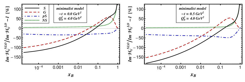
Figure 6: Relative NLO corrections to the imaginary part of the flavor singlet TFF ${\mathcal{F}}^{{\text{S}}}_{\text{V}}$ (solid) broken down to the gluon (dashed), pure singlet quark (dash-dotted) and ‘non-singlet’ quark (dotted) at $t=0\,{\rm GeV}^{2}$ (left panel) and $t=-0.5\,{\rm GeV}^{2}$ (right panel) at the initial scale ${\cal Q}_{0}^{2}=4\,{\rm GeV}^{2}$.

Our discussion of the imaginary part for the flavor singlet TFF, evaluated from the minimalist GPD model, is visualized in Fig. 6 for $t=0$ (left panel) and $t=-0.5\,{\rm GeV}^{2}$ (right panel). Here we display the relative NLO corrections, evaluated analogously to (5.38), that arise from the gluonic NLO coefficients (dashed curves), the pure singlet quark (short dash-dotted curves), the remaining quark part (dotted curves), and the net contribution (solid curves). Clearly, the large-$x_{\rm B}$ asymptotic arises from the valence content, compare with Fig. 4, where the contributions from the ‘non-singlet’ hard scattering amplitude dominate the net result. As stated, in the valence region the non-singlet contribution is moderately positive and the pure singlet is negative, while it turns out that in our model the gluonic one yields a rather sizeable positive correction. In the small-$x_{\rm B}$ region the gluons dominate in our model and their contributions are essentially governed by the $j=0$ pole. These large corrections increase further with growing $-t$ since the ‘pomeron’ pole at $j=0.247+0.15t$ gets slightly softer. Note that the shape of the curves in the small-$x_{\rm B}$ region is governed by the functional forms as it arises from the $j=0$ pole contributions, e.g., shown in (5.50), and R-ratios (5.41c). For our model the quark content vanishes in the $x_{\rm B}\to 0$ limit while the gluon ones is as sizable as $-144\%$ [$-233\%$] for $t=-0$ $[t=-0.5{\rm GeV}^{2}]$.

• Model dependency.

Finally, let us also demonstrate in Fig. 7 for the modulus (left panel) and the phase change (right panel), defined as in (5.27), that the NLO corrections in the flavor singlet sector are rather model dependent. We display again the minimalist model (solid curves) and the nnl-SO(3) PW model as specified in Tab. 7 (dashed curves) with the narrow DA (5.28) for $t=-0\,{\rm GeV}^{2}$ (thick curves) and $t=-0.5\,{\rm GeV}^{2}$ (thin curves). For the minimalist model the corrections to the modulus are smaller than $100\%$ and they become negative in the small $x_{\rm B}$ region. As we have discussed the reduction of relative NLO corrections to the modulus in the large-$x_{\rm B}$ region is a naturally consequence of analyticity, i.e., the validity of the DR. Compared to Fig. 6, the relative NLO corrections to the modulus in the small-$x_{\rm B}$ region are looking rather mild (solid curves). Note that this is caused by the negative size of the NLO contribution, dominated by the $j=0$ pole, which overcompensates the positive LO contribution and induces a phase difference of $\pi$ in the small-$x_{\rm B}$ asymptotic. Entirely different features appear for our nnl-SO(3) PW model. Here the size of NLO corrections is for $t=0$ positive in the small-$x_{\rm B}$ region and gets for a softer ‘pomeron’ behavior at $t=-0.5\,{\rm GeV}^{2}$ negative, where the phase difference slightly increases. On the other hand we have now huge corrections to the moduli around the valence region, see dashed curves, which are caused by strong evolution effects in the gluon sector.

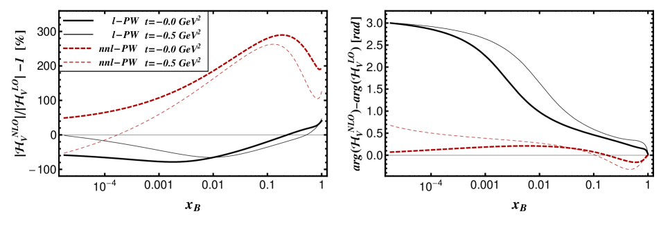
Figure 7: Relative NLO corrections to the modulus (left panel) and phase (right panel) for the flavor singlet TFF ${\mathcal{H}}^{\text{S}}_{V}$ for our minimalist (l-SO(3) PW, asymptotic DA) model (solid curves) and a nnl-SO(3) PW model with a narrow DA (dashed curves) at $t=0\,{\rm GeV}^{2}$ (thick curves) and $t=-0.5\,{\rm GeV}^{2}$ (thin curves) at the initial scale ${\cal Q}_{0}^{2}=4\,{\rm GeV}^{2}$.

5.3.3 Comparison of DVMP and DVCS NLO corrections

We add that an estimate of radiative corrections for DVCS can be generically done in an analog manner, providing us a deeper understanding of various model dependent studies [112, 113, 54, 114]. To adopt it to our notation here, we write the quark conformal moments (127,128) form [54] as

$${}^{\sigma}\!c_{j}^{\rm DVCS} \!\!\!=\!\!\! 1+\frac{\alpha_{s}(\mu_{\rm R})}{2\pi}C_{\text{F}}\,^{\sigma}\!c_{j}^{(1,\text{F})}+O(\alpha_{s}^{2})\,,$$ (5.51a)

$${}^{\sigma}\!c_{j}^{(1,\text{F})} \!\!\!=\!\!\! \bigg{[}\ln\frac{{\cal Q}^{2}}{\mu_{\rm F}^{2}}-\frac{\gamma^{(0,\text{F})}_{j}}{4}-\frac{3(j+1)_{2}+1}{2(j+1)_{2}}\bigg{]}\frac{(-1)\gamma^{(0,\text{F})}_{j}}{2}-\frac{27}{8}+\frac{(11+2\sigma)(j+1)_{2}+4}{4[(j+1)_{2}]^{2}}\,,\qquad\qquad$$ (5.51b)

where signature $\sigma=+1$ and $\sigma=-1$ applies for the twist-two CFFs ${\cal F}\in\{{\cal H},{\cal E}\}$ and ${\cal F}\in\{\widetilde{\cal H},\widetilde{\cal E}\}$, respectively. Already the similarity of the most singular terms with the TFF estimate (5.38) implies that the NLO corrections have similar features. This is not the case in the flavor singlet channel, where the conformal moments read as follows

$${}^{\sigma}\!\mbox{\boldmath$c$}_{j}^{\rm DVCS} \!\!\!=\!\!\! (1,0)+\frac{\alpha_{s}(\mu_{\rm R})}{2\pi}\left(C_{\text{F}}\,^{\sigma}\!c_{j}^{(1,\text{F})},\frac{2n_{f}}{j+3}\,^{\sigma}\!c_{j}^{(1,n_{f})}\right)+O(\alpha_{s}^{2})\,,$$ (5.52a)

$${}^{\sigma}\!c_{j}^{(1,n_{f})} \!\!\!=\!\!\! \left[\ln\frac{{\cal Q}^{2}}{\mu_{\rm F}^{2}}-\frac{\gamma^{(0,\text{F})}_{j}}{2}-\frac{5}{2}\right]\frac{j+3}{2}\,\frac{(-1)^{{\Sigma{\text{G}}}^{\sigma}}\!\gamma^{(0,nf)}_{j}}{2}+\frac{1+\sigma}{2(j+1)_{2}}\,,$$ (5.52b)

where we use the notation $${}^{{\Sigma{\text{G}}}^{+}}\!\gamma^{(0,nf)}_{j}\equiv^{{\Sigma{\text{G}}}}\!\gamma^{(0,nf)}_{j} {}^{{\Sigma{\text{G}}}^{-}}\!\gamma^{(0,nf)}_{j}=-2j/(j+1)_{2}$$ and  .

• Flavor non-singlet channel.

Replacing the anomalous dimensions in (5.51) by (5.14) yields the generic estimate

$$\frac{\Im{\rm m}\,^{\text{NS}}{\mathcal{F}}^{\rm NLO}_{\gamma}}{\Im{\rm m}\,^{\text{NS}}{\mathcal{F}}^{\rm LO}_{\gamma}}=1+\frac{\alpha^{\rm NLO}_{s}(\mu_{\rm R})}{2\pi}\,\frac{2}{3}\left\{\left(2\ln\frac{{\cal Q}^{2}}{\mu_{\rm F}^{2}}+\frac{\ell^{\prime\prime}_{F}(\xi,t)}{\ell^{\prime}_{F}(\xi,t)}-3\right)\ell^{\prime}_{F}(\xi,t)-\frac{27}{4}+\cdots\right\}$$ (5.53a)

for the DVCS flavor non-singlet channel. As in the TFF estimate (5.38), the behavior in the large-$$x_{\rm B} -\ell^{\prime}_{F}(\xi,t) \ell^{\prime\prime}_{F}(\xi,t)\approx\ell^{\prime\,2}_{F}(\xi,t)$$ region is dictated by a logarithmical growth of , where the squared term is universal. Furthermore, neglecting evolution effects, we find in the valence region a moderate NLO correction

$$\frac{\Im{\rm m}\,^{\text{NS}}{\mathcal{F}}^{\rm NLO}_{\gamma}}{\Im{\rm m}\,^{\text{NS}}{\mathcal{F}}^{\rm LO}_{\gamma}}-1\sim\frac{\alpha_{s}}{2\pi}(-9/2)\approx-25\%\quad\mbox{for}\quad{\cal Q}_{0}^{2}=4\,{\rm GeV}^{2}\,,$$ (5.53b)

which size is comparable with our findings for flavor non-singlet TFFs, however, it is now negative. In the small-$$x_{\rm B} j=-1 x_{\rm B}\to 0$$ region non-singular terms, which contain a pole at yield large relative NLO corrections, however, are phenomenological unimportant. The exact asymptotics for a minimal GPD model can be trivially found from the conformal moments,

$$\frac{\Im{\rm m}\,^{\text{NS}}{\mathcal{F}}^{\rm NLO}_{\gamma}}{\Im{\rm m}\,^{\text{NS}}{\mathcal{F}}^{\rm LO}_{\gamma}} \!\!\!\stackrel{{\scriptstyle x_{\rm B}\to 0}}{{=}}\!\!\! 1+\frac{\alpha_{s}}{2\pi}\,\frac{2}{3}\Bigg{\{}4\left[S_{1}(\alpha(t))\right]^{2}-\frac{2S_{1}(\alpha(t))}{\alpha(t)[1+\alpha(t)]}-9+\frac{(4+\sigma)\alpha(t)[1+\alpha(t)]+2}{\alpha^{2}(t)[1+\alpha(t)]^{2}}\Bigg{\}}.\qquad\quad$$ (5.53c)

Compared to the flavor non-singlet TFFs, given in (5.39), we have rather similar features, which, however, differ in some details. Again caused by the first and second order pole at $\alpha(t)=0$, they become huge and positive for smaller values of $\alpha(t)$, they vanish for $\alpha(t)\sim 0.5$, while for $\alpha(t)\sim 1$ we find that they are negative and smaller than in the valence region. The differences of even and odd signature sector are not essential.

• Flavor singlet channel for even signature.

In the large-$x_{\rm B}$ region the signature even singlet contribution is as in DVMP entirely determined by the valence quark content and is positive. Hence, its process independent features may be read off from (5.53a). In the valence region both the quark and gluonic component yields a negative correction, which looks rather harmless. For GPD models that only evolve weakly in the valence region we can immediately quote the crude approximation

$$\frac{\Im{\rm m}\,^{\text{S}}{\mathcal{F}}^{\rm NLO}_{\gamma}}{\Im{\rm m}\,^{\text{S}}{\mathcal{F}}^{\rm LO}_{\gamma}}-1\stackrel{{\scriptstyle x_{\rm B}=\overline{x}_{\rm B}}}{{\approx}}\frac{\alpha_{s}}{2\pi}\left\{-\frac{9}{2}-\frac{5}{4}\,\frac{n_{f}\,F^{\text{G}}(\xi,\xi,\cdots)}{F^{\Sigma}(\xi,\xi,\cdots)}+\cdots\right\}\quad\mbox{for}\quad{\cal Q}_{0}^{2}=4\,{\rm GeV}^{2}\,.$$ (5.54)

The gluonic induced correction is determined by the ratio $n_{f}F^{\text{G}}(\xi,\xi,\cdots)/F^{\Sigma}(\xi,\xi,\cdots)$. This model dependent ratio may be of order one and so the gluonic component gives a moderate contribution to the quark induced one, which decreases the flavor non-singlet estimate of $\sim-25\%$ further. Since a $j=0$ pole is absent in the conformal moments (5.52), also the corrections in the small-$x_{\rm B}$ region possess now different qualitative features than for DVMP. For the minimalist GPD model they are roughly given in the presence of a ‘pomeron’ pole by

$$\frac{\Im{\rm m}\,^{\text{S}}{\mathcal{F}}^{\rm NLO}_{\gamma}}{\Im{\rm m}\,^{\text{S}}{\mathcal{F}}^{\rm LO}_{\gamma}}-1\stackrel{{\scriptstyle x_{\rm B}\to 0}}{{\approx}}\frac{\alpha_{s}}{2\pi}\left\{-2-\frac{4}{3}\frac{n_{f}\,{\rm Res}F^{\text{G}}_{j}|_{j=\alpha^{\text{G}}-1}}{{\rm Res}F^{\Sigma}_{j}|_{j=\alpha^{\rm sea}-1}}\left(\frac{x_{\rm B}}{2}\right)^{\alpha^{\rm sea}-\alpha^{\text{G}}}+\cdots\right\}\,,$$ (5.55)

where different coefficients appear in other models. To describe DVCS or deep inelastic scattering data from the H1 and ZEUS collaboration in LO approximation, one has usually $\alpha^{\text{G}}>\alpha^{\rm sea}>1$ at our input scale and so the NLO corrections are sizeable and negative. In contrast to DVMP a ‘hard’ gluon yields now sizeable corrections. However, we should emphasize that the rather large LO value of $\alpha^{\text{G}}$ arise simply from the fact that the role of the $j=0$ pole in the evolution operator is then less important and so the pQCD ${\cal Q}^{2}$-evolution can be brought in agreement with the observed one in deep inelastic scattering. At NLO the gluon PDF/GPD is also directly controlled which leads in general to a smaller value of $\alpha^{\text{G}}$. Taking the PDF reparameterization consistently into account in building GPD models, one may expect smaller radiative corrections for DVCS. What matters for phenomenology is not the estimated size of radiative corrections of some GPD models, rather how pQCD connects the different processes of interest in the small-$x_{\rm B}$ region. This is a kind of fine tuning problem and only after data are successfully described on can quantify reparameterization effects.

6 Summary and conclusions

We have systematized the theoretical framework for the perturbative treatment of the DVMP process. In particular we have expressed the differential cross section in terms of physically motivated TFFs. We have also considered the case that the polarization of the final nucleon state is observed, which offers at least in principle the possibility for a complete measurement of the TFFs. Furthermore, we have recalculated the pure singlet quark part for DV​$V_{L}^{0}$P and presented a set of NLO formulae which allows to easily implement the radiative corrections, which are classified into flavor non-singlet contributions with defined signature and flavor singlet contributions. Also, we have considered besides the common momentum fraction representation the dispersive approach and conformal partial wave expansion in terms of a Mellin-Barnes integral. We have evaluated the imaginary parts of NLO hard scattering amplitudes and their conformal moments, which are needed for implementing the radiative corrections into an existing GPD fitting code. In this way, we represented the conformal moments by common Mellin moments, which allowed us to calculate them analytically in terms of rational functions and harmonic sums. We also pointed out that the analytic continuation can be numerically performed by means of single or double dispersion relations. Our presentation of the NLO corrections to the hard scattering amplitude, essentially given in terms of building blocks, can be easily adapted to mixed representations. This is possibly useful for the case that the meson DA is much broader or narrower than the asymptotic one.

NLO corrections to the hard scattering amplitudes for phenomenologically important DV$\!V_{L}$P and DV$\!P\!S$P reactions were presented in such a manner that they match existing conventions, used in DVCS and for the evolution operator or kernels. Here, only for DV$\!\eta$P, having odd $t$-channel charge parity and odd intrinsic parity, the NLO contributions to the hard scattering amplitudes for both the singlet quark DA, i.e., its pure singlet part $\gamma^{\ast}(q\bar{q})^{(-)}\to(q\bar{q})^{\mathrm{pS}}$, and gluonic DA are still missing. These reactions were measured or are planned to be measured in near future at COMPASS II and JLAB@12 ${\rm GeV}$. Consequently, for the more experimental challenging DV$\!h_{0}$P reaction ($h_{0}=1^{+-}$), having even $t$-channel charge parity and odd intrinsic parity, both the pure singlet quark-quark [$\gamma^{\ast}(q\bar{q})^{\mathrm{pS}}\to(q\bar{q})^{(-)}$] and the gluon-quark [$\gamma^{\ast}gg\to(q\bar{q})^{(-)}$] channel remain unknown at NLO. We also add that for DV$\!f_{0}$P ($f_{0}=0^{++}$), having odd $t$-channel charge parity and even intrinsic parity, all NLO ingredients including the corresponding pure singlet quark and gluon scalar meson DA contributions are obtained from those of DV$\!V_{L}^{0}$P by an exchange of the in- and out-momentum fraction variables. Whether these reactions can be accessed in high luminosity experiments at JLAB, remains so far unclear to us. Finally, we emphasize that the NLO formulae can be also utilized for crossed processes, e.g., for exclusive Drell-Yan processes $\pi N\to N^{\prime}\gamma^{\ast}_{L}$ [83]. So far, however, it remains questionable if such reactions can be observed in planned Drell-Yan measurements at COMPASS II.

Furthermore, we comprehensively analyzed the role of radiative NLO corrections that arises from the hard scattering part, where for the first time we also gave an analytical discussion that is based on generally expected GPD properties. We observed that perturbative corrections in the large-$x_{\rm B}$ asymptotics appear in the same manner in both DVCS and DVMP. We add that the resummation of so-called soft and collinear contributions, proposed for DVCS in [148], seems to be only useful in this region. For GPD models that evolve only weakly in the valence region we found that the corrections in the valence region in both DVCS and DVMP are more or less harmless, however, they have different sign. In the presence of ‘pomeron’ behavior the size of radiative corrections in the small-$x_{\rm B}$ region is very model dependent, since it is crucially governed by the effective ‘pomeron’ intercepts of both the quark singlet and gluon trajectories and also in a more moderate manner on the skewness effect. Hence, only a fit to data can tell us how large reparametrization effects are.

To get a handle on GPDs from present (and future) longitudinal DVMP and transversal DVCS measurements in a reliable manner, one certainly should in the first place utilize the collinear framework, where at least factorization was proven. In such analyses evolution must definitely be consistently included. We add that one usually assumes that the scheme (and framework) dependent meson DA is known, but even in the case of the pion DA rather different models were proposed [149, 150, 151, 152, 153, 131, 154, 155] which, unfortunately, can be discriminated only partially by present experimental pion form factor [156, 157, 158, 159] and pion-to-photon transition form factor [160, 161, 162, 163] data and lattice results [164]. For light vector meson DAs only QCD sum rule results [165, 166], see also references therein, and AdS/QCD model predictions [131] are known to us.

Based on present phenomenological experience in the description of DVCS and DV$\!V^{0}_{L}$P processes in the small-$x_{\rm B}$ region [55, 50] we are rather optimistic that a global description of these processes is reachable at NLO. One arrives at the same conclusion if one considers the results based on the handbag approach [51, 52] and their confrontation with DVCS data [50, 61]. Analogously, the phenomenological findings in the handbag approach [51, 52] and its confrontation with DVCS [50, 60, 61], which indicates that a description of such processes might be feasible in the valence region. The description of the DV$\!V^{0}_{L}$P data from the CLAS collaboration in the large-$x_{\rm B}$ region requires a separate study. In the case of DV$\!\pi^{+}$P we have also phenomenological constraints for the pion DA that arise from the electromagnetic pion and photon-to-pion transition form factor. A simultaneous description of these form factor and DV$\!\pi^{+}$P data in the pQCD framework remains an interesting problem.

Acknowledgements

We are indebted to K. Kumerički for many discussions and numerical implications of DVMP formulae, which were used by us for cross checks. We also like to thank H. Avakian, N. Kivel, P. Kroll, S.V. Mikhailov, A.V. Pimikov, and N. G. Stefanis for discussions one some selected topics. This work was supported in part by the Joint Research Activity Study of Strongly Interacting Matter (acronym HadronPhysics3, Grant Agreement No. 283286) under the Seventh Framework Program of the European Community; by the Croatian Ministry of Science, Education and Sport under the contract no. 098-0982930-2864; and by the German Ministry of Science and Education (BMBF grant OR 06RY9191 and 05P12WRFTE).

Appendix A Conventions

In order to use the results from the literature or to compare them to our results, it is important to be aware of the different conventions used. The definitions of GPDs and DAs uniquely determine the hard scattering amplitudes, evolution kernels and their anomalous dimensions. One often encounters these elements separately in the literature. In this section we spell out our definitions, adopted from [22, 107], and show how ours, those in [9], and in [10] are connected to each other.

A.1 GPD definitions

GPDs are defined as expectation values of renormalized light-ray operators, sandwiched between a polarized in- and out-proton state [1, 2, 3]. The most often encountered definitions for twist-two GPDs read in the notation of [22, 107] for unpolarized partons (parity even operators)

$$q(x,\eta,t,\mu^{2}) \!\!\!=\!\!\! \int\frac{d\kappa}{2\pi}\>e^{ix(P\cdot n)\kappa}\langle s_{2},p_{2}|\bar{q}(-\kappa n)\gamma^{+}q(\kappa n)|p_{1},s_{1}\rangle_{(\mu^{2})},$$ (A.1a)

$$G(x,\eta,t,\mu^{2}) \!\!\!=\!\!\! \frac{4}{P\cdot n}\int\frac{d\kappa}{2\pi}\>e^{ix(P\cdot n)\kappa}\langle s_{2},p_{2}|G^{+\mu}_{a}(-\kappa n)G_{a\mu}^{\;\;\>+}(\kappa n)|p_{1},s_{1}\rangle_{(\mu^{2})},$$ (A.1b)

and for polarized ones (parity odd operators)

$$\Delta q(x,\eta,t,\mu^{2}) \!\!\!=\!\!\! \int\frac{d\kappa}{2\pi}\>e^{ix(P\cdot n)\kappa}\langle s_{2},p_{2}|\bar{q}(-\kappa n)\gamma^{+}\gamma_{5}q(\kappa n)|p_{1},s_{1}\rangle_{(\mu^{2})},$$ (A.2a)

$$\Delta G(x,\eta,t,\mu^{2}) \!\!\!=\!\!\! \frac{4}{P\cdot n}\int\frac{d\kappa}{2\pi}\>e^{ix(P\cdot n)\kappa}\langle s_{2},p_{2}|G^{+\mu}_{a}(-\kappa n)i\epsilon^{\perp}_{\mu\nu}G_{a}^{\nu+}(\kappa n)|p_{1},s_{1}\rangle_{(\mu^{2})}.$$ (A.2b)

Here

$$P=p_{1}+p_{2}\;,\quad\Delta=p_{2}-p_{1}\;,\quad t\equiv\Delta^{2}\;,\qquad\eta=-\frac{\Delta\cdot n}{P\cdot n}\;,\quad\epsilon^{\perp}_{\mu\nu}=\epsilon_{\mu\nu\alpha\beta}\,n^{\ast\alpha}n^{\beta}\;,\quad\epsilon^{0123}=1,$$

$n^{\mu}$ and $n^{\ast\mu}$ are (conventional) light-like vectors with $n\cdot n^{\ast}=1$, where $a^{+}\equiv a\cdot n$ projects on the +-component. The quark GPD definitions are chosen in such a manner that they coincide with the PDF definitions in terms of light-ray operators in the forward limit $p_{2}\to p_{1}\equiv p$, i.e., $P=2p$, $s_{2}\to s_{1}\equiv s$, while for the gluon an additional factor $1/x$ appears in the PDF definition, see, e.g., [167]. We note that the momentum fraction $\eta$ is often equated with $\xi$, which plays in DVMP the role of a scaling variable and that this variable depends on the conventional choice of the light-cone vector. The sign in the $\eta$ definition is not chosen uniformly in the literature. Here, and in the following $\eta$ is taken to be non-negative. Furthermore, often one denotes with $P$ the average of $p_{1}$ and $p_{2}$. The target spin content of unpolarized (A.1) and polarized (A.2) GPDs is parameterized in terms of form factors

$$q \!\!\!=\!\!\! \overline{u}\,_{2}\!\left[\frac{\gamma^{+}}{P^{+}}H^{q}+\frac{i\sigma^{+\mu}\Delta_{\mu}}{P^{+}\,2M}E^{q}\right]\!u_{1}\,,\quad\phantom{\Delta}\;\;G=\overline{u}\,_{2}\!\left[\frac{\gamma^{+}}{P^{+}}H^{\text{G}}+\frac{i\sigma^{+\mu}\Delta_{\mu}}{P^{+}\,2M}E^{\text{G}}\right]\!u_{1}\,,$$ (A.3a)

$$\Delta q \!\!\!=\!\!\! \overline{u}\,_{2}\!\left[\frac{\gamma^{+}\gamma_{5}}{P^{+}}\widetilde{H}^{q}+\frac{\Delta^{+}\,\gamma_{5}}{P^{+}\,2M}\widetilde{E}^{q}\right]\!u_{1}\,,\quad\Delta G=\overline{u}\,_{2}\!\left[\frac{\gamma^{+}\gamma_{5}}{P^{+}}\widetilde{H}^{\text{G}}+\frac{\Delta^{+}\,\gamma_{5}}{P^{+}\,2M}\widetilde{E}^{\text{G}}\right]\!u_{1}\,,$$ (A.3b)

where Dirac spinors $u_{i}\equiv u(p_{i},s_{i})$ are normalized as $\overline{u}\,(p,s)\gamma^{\mu}u(p,s)=2p^{\mu}$. Hence, in the forward limit the form factors of the target helicity flip contributions vanish and $q=H^{q},{\text{G}}=H^{\text{G}}$ and $\Delta q=\widetilde{H}^{q},\Delta{\text{G}}=\widetilde{H}^{\text{G}}$ GPDs reduce as shown in (A.4,A.5) to unpolarized and polarized PDFs, respectively. These definitions agree with those in [9] and in [10]. See also remarks in [9] about some mismatches with other definitions.

Note that GPDs and PDFs from operator definitions have the support $x\in[-1,1]$ and, thus, a quark GPD/PDF contains both quark and antiquark contributions:

$$q(x\geq 0,\eta=0,t=0,\mu^{2}) \!\!\!=\!\!\! q(x,\mu^{2})\,,\phantom{\Delta}\quad q(x\leq 0,\eta=0,t=0,\mu^{2})=-\bar{q}(-x,\mu^{2})\,,\phantom{\Delta\Delta}$$ (A.4a)

$$\Delta q(x\geq 0,\eta=0,t=0,\mu^{2}) \!\!\!=\!\!\! \Delta q(x,\mu^{2})\,,\quad\Delta q(x\leq 0,\eta=0,t=0,\mu^{2})=\Delta\bar{q}(-x,\mu^{2})\,.\phantom{\Delta\Delta}$$ (A.4b)

In the forward limit the gluon GPD $(\Delta){\text{G}}$) as defined in (A.1b,A.2b) yields the standard unpolarized (polarized) gluon PDF $g$ ($\Delta g$) in both regions $x\geq 0$ and $x\leq 0$, where, however, gluon PDFs have an additional $x$ factor:

$$G(x\geq 0,\eta=0,t=0,\mu^{2})=xg(x,\mu^{2})\,,\quad\Delta G(x\geq 0,\eta=0,t=0,\mu^{2})=x\Delta g(x,\mu^{2})\,.$$ (A.5)

Because of Bose symmetry gluon GPDs (PDFs) have definite symmetry behavior under $x\to-x$ reflection,

$$G(-x,\cdots)=G(x,\cdots)\quad\mbox{and}\quad\Delta G(-x,\cdots)=-\Delta G(x,\cdots)\,.$$ (A.6)

Gluon GPDs have even charge parity, while a quark GPD basis (3.1) with definite charge parity reads explicitly as

$$F^{{q^{(\pm)}}}(x,\cdots) \equiv F^{q}(x,\cdots)\mp F^{q}(-x,\cdots)\quad\mbox{for}\quad F\in\{H,E\}\,,$$ (A.7a)

$$F^{{q^{(\pm)}}}(x,\eta,t) \equiv F^{q}(x,\cdots)\pm F^{q}(-x,\cdots)\quad\mbox{for}\quad F\in\{\widetilde{H},\widetilde{E}\}\,,$$ (A.7b)

where $F^{{q^{(+)}}}$ and $F^{{q^{(-)}}}$ refer to even and odd charge parity, respectively. A quark GPD $F^{q}$ can be decomposed in antiquark ($-1\leq x\leq-\eta$), meson-like ($-\eta\leq x\leq\eta$ ), and quark ($\eta\leq x\leq 1$) contributions, which one may write in analogy to PDF terminology (A.4) as

$$F^{q}(x,\cdots)=\mp F^{\overline{q}}(-x\geq\eta,\cdots)+F^{q}(|x|\leq\eta,\cdots)+F^{q}(x\geq\eta,\cdots)\,,$$ (A.8a)

where $$- + F\in\{H,E\} F\in\{\widetilde{H},\widetilde{E}\} \eta\leq x$$ and applies for unpolarized quark GPDs and polarized quark GPDs , respectively. Hence, charge even (odd) GPDs contain for the sum (difference) of quark and aniquark GPDs,

$$F^{{q^{(\pm)}}}(x\geq\eta,\cdots)=F^{q}(x\geq\eta,\cdots)\pm F^{\overline{q}}(x\geq\eta,\cdots)\,.$$ (A.8b)

We note that in PDF terminology a quark PDF is decomposed into valence and sea quark contributions, where the latter is equated with the antiquark ones. In phenomenology it is common to adopt this PDF terminology and we, therefore, write the charge even quantities in terms of valence quarks and antiquarks:

$$F^{q(+)}(x\geq\eta,\eta,\cdots) \!\!\!=\!\!\! F^{q^{\rm val}}(x,\eta,\cdots)+2F^{\bar{q}}(x,\eta,\cdots)\,,$$ (A.8c)

$$F^{q(-)}(x\geq\eta,\eta,\cdots) \!\!\!=\!\!\! F^{q^{\rm val}}(x,\eta,\cdots)\,,$$ (A.8d)

where charge odd GPDs have only valence quark content.

Finally, a group theoretical SU$(n_{f})$ decomposition of quark GPDs, e.g., for $n_{f}=3$ $(n_{f}=4)$

$$F^{0} \!\!\!=\!\!\! F^{u}+F^{d}+F^{s}\,(+F^{c})$$ (A.9a)

$$F^{3} \!\!\!=\!\!\! F^{u}-F^{d}$$ (A.9b)

$$F^{8} \!\!\!=\!\!\! F^{u}+F^{d}-2F^{s}$$ (A.9c)

$$(F^{15} \!\!\!=\!\!\! F^{u}+F^{d}+F^{s}-3F^{c})\,.$$ (A.9d)

is utilized to solve the mixing problem of charge even quark and gluon GPDs. For flavor singlet $0^{(+)}$ quark and gluon GPDs we utilize a vector valued GPD, defined in (3.5). Note that the unpolarized $0^{(+)}$ GPD in the charge even sector is labeled by the superscript $\Sigma$. Hard scattering amplitudes and evolution kernel may also contain a pure singlet quark part. In our notation $\Sigma$ refers always to the net contribution, containing both the group theoretical part $0^{(+)}$ and the pure singlet quark piece, see the TFF decomposition for a neutral vector meson TFF decomposition (2.23). The sum of gluon and $\Sigma$ contribution is labeled by superscript S.

A.2 Evolution kernels

The scale dependence of flavor non-singlet or charge odd DAs is governed by the well known Efremov-Radyushkin-Brodsky-Lepage (ER-BL) evolution equation which has the following form

$$\mu^{2}\frac{d}{d\mu^{2}}\varphi^{\text{A}}(u,\mu^{2})=V\left(u,v|\alpha_{s}(\mu)\right)\stackrel{{\scriptstyle v}}{{\otimes}}\varphi^{\text{A}}(v,\mu^{2})\,,\quad f\stackrel{{\scriptstyle v}}{{\otimes}}g\equiv\int_{0}^{1}\!dv\,fg$$ (A.10)

for $\text{A}\in\{{{\rm NS}^{(+)}},{q^{(-)}}\}$. In this case we have the restriction $0\leq v\leq 1$, and the support of the evolution kernel simplifies to

$$V(u,v|\alpha_{s})=\theta(v-u)f(u,v|\alpha_{s})+\theta(\overline{u}\,-v)\overline{f}(u,v|\alpha_{s})+\left\{{u\to\overline{u}\,\atop v\to\overline{v}\,}\right\}\,.$$ (A.11)

Here, the $\overline{f}$-part stems from quark-antiquark mixing and appears at NLO [1]. Due to the appearance of $\overline{f}$, the evolution kernels for symmetric or antisymmetric DAs differ in higher orders from each other, i.e., it depends on the signature. The LO approximation of the ER-BL kernel, known from 1980’s, (see [85] and references therein) is given in (3.23).

For flavor non-singlet or a charge odd GPD $F$ the evolution equation can be obtained from the quoted one by replacing the $0\leq v\leq 1$ restriction by the support of the kernel [104]:

$$\theta(v-u)\rightarrow\Theta(u,v)=\theta\!\left(1-\frac{u}{v}\right)\theta\!\left(\frac{u}{v}\right){\rm sign}(v)\,.$$

In the variables we are using, i.e., $u=(\eta+x)/2\eta$ and $v=(\eta+y)/2\eta$, the evolution equation reads

$$\mu^{2}\frac{d}{d\mu^{2}}F^{\text{A}}(x,\eta,t,\mu^{2})=\int_{-1}^{1}\!\frac{dy}{2\eta}\,^{\sigma}V\!\left(\!\frac{\eta+x}{2\eta},\frac{\eta+y}{2\eta}\Big{|}\alpha_{s}(\mu)\!\!\right)F^{\text{A}}(y,\eta,t,\mu^{2})$$ (A.12)

with the proper signature $\sigma(\text{A})$ for $\text{A}\in\{{\rm NS}^{(\pm)},{q^{(-)}}\}$.

In the flavor singlet channel the evolution of our vector valued GPD $F$, given in (3.5), reads

$$\mu^{2}\frac{d}{d\mu^{2}}\mbox{\boldmath$F$}(x,\eta,t,\mu^{2})=\int_{-1}^{1}\!\frac{dy}{2\eta}\,\mbox{\boldmath$V$}\!\left(\!\frac{\eta+x}{2\eta},\frac{\eta+y}{2\eta};\eta\Big{|}\alpha_{s}(\mu)\!\right)\cdot\mbox{\boldmath$F$}(y,\eta,t,\mu^{2})\,.$$ (A.13)

The quark entry of the GPD vector is the sum over all charge even quark GPDs (A.7) and it reads together with the evolution matrix as

$$\left(\sum_{q}{F^{q^{(+)}}}\atop{F^{\rm G}}\right)(\cdots)\quad\mbox{and}\quad\mbox{\boldmath$V$}(u,v;\eta|\alpha_{s})=\left(\!\!\!\begin{array}[]{cc}\phantom{2\eta\,}{{}^{\Sigma\Sigma}}V&{{}^{\Sigma{\text{G}}}}V/2\eta\\ 2\eta\,{{}^{{\text{G}}\Sigma}}V&{{}^{{\text{G}}{\text{G}}}V}\phantom{/2\eta}\end{array}\!\!\!\right)\!\!(u,v|\alpha_{s})\,,$$ (A.14a)

respectively. Exploiting symmetry of the GPDs the entries can be represented as

$${{}^{\text{AB}}V}(u,v|\alpha_{s})=\theta(v-u)\,{{}^{\text{AB}}}v(u,v|\alpha_{s})\pm\left\{{u\to\bar{u}\atop v\to\bar{v}}\right\}\mbox{\ for\ }\left\{{\text{A}=\text{B}\atop\text{A}\not=\text{B}}\right.,$$ (A.14b)

where the quark-quark channel consists of the charge even non-singlet, with definite signature, and the pure singlet part

$${{}^{\Sigma\Sigma}}v(u,v|\alpha_{s})={{}^{\sigma}}v(u,v|\alpha_{s})+{{}^{\mathrm{pS}}}v(u,v|\alpha_{s})\quad\sigma=\left\{{+\mbox{ for }F\in\{H,E\}\atop-\mbox{ for }F\in\{\widetilde{H},\widetilde{E}\}}\right..$$ (A.14c)

With the GPD conventions (A.1,A.2) the LO kernel reads as in [85], shown for unpolarized parton GPDs in (3.24). Various other authors published these LO kernels, too. Be aware that the functional form can differ, which only should affect the non-physical sector. Those in (3.24) are the kernels from [169], while the improved ones provide for both kinds of moments (even and odd) polynomials [170]. These kernels were used as one ingredient to construct the NLO corrections for the entries in (A.14a) [107].

With these specifications, we have checked that the forward limit of the evolution equation (A.13) yields for positive $x$ nothing but the flavor singlet DGLAP equation,

$$\mu^{2}\frac{d}{d\mu^{2}}\left({\Sigma(x,\mu^{2})\atop xg(x,\mu^{2})}\right)=\int_{x}^{1}\!\frac{dy}{y}\,\left(\!\!\!\begin{array}[]{cc}\phantom{2\eta\,}{{}^{\Sigma\Sigma}}p\big{(}\frac{x}{y}|\alpha_{s}\big{)}&\frac{1}{y}\,{{}^{\Sigma{\text{G}}}}p\big{(}\frac{x}{y}|\alpha_{s}\big{)}\\ x\,{{}^{{\text{G}}\Sigma}}p\big{(}\frac{x}{y}|\alpha_{s}\big{)}&\frac{x}{y}\,{{}^{{\text{G}}{\text{G}}}}p\big{(}\frac{x}{y}|\alpha_{s}\big{)}\end{array}\right)\cdot\left({\Sigma(y,\mu^{2})\atop y\,g(y,\mu^{2})}\right)\,,$$ (A.15)

where the well-known expressions of LO kernels, see, e.g. [171], follows from (3.24), showing that definitions and diagrammatical results as we use them here are consistent. The same holds true for the NLO corrections to the entries given in [107] and those for splitting kernels from Ref. [171]. Be aware that the flavor singlet evolution kernels for $H/E$ and $\widetilde{H}/\widetilde{E}$ type GPDs are different.

Other forms of evolution equations are also known, e.g., with non-symmetrized quark GPDs (A.1a,A.2a). However, as long as one respects the proper symmetry for gluon GPDs, only charge even quark GPDs have cross talk with gluonic GPDs, while the charge odd quark part decouples and evolves autonomously. Often the normalization remains confusing, if conventions are not entirely spelled out. By rescaling of quark and gluon GPDs with constants $a$ and $b$, respectively, the off diagonal entries in the evolution kernel change, too,

$$\left(\sum_{q}{F^{q^{(+)}}}\atop{F^{\rm G}}\right)\rightarrow\left(a\,\sum_{q}{F^{q^{(+)}}}\atop b\,{F^{\rm G}}\right)\;\;\mbox{implies:}\;\;\left(\!\!\!\begin{array}[]{cc}\phantom{2\eta\,}{{}^{\Sigma\Sigma}}V&{{}^{\Sigma{\text{G}}}}V/2\eta\\ 2\eta\,{{}^{{\text{G}}\Sigma}}V&{{}^{{\text{G}}{\text{G}}}V}\phantom{/2\eta}\end{array}\!\!\!\right)\rightarrow\left(\!\!\!\begin{array}[]{cc}\phantom{2\eta\,}{{}^{\Sigma\Sigma}}V&\frac{a}{b}\,{{}^{\Sigma{\text{G}}}}V/2\eta\\ 2\eta\,\frac{b}{a}\,{{}^{{\text{G}}\Sigma}}V&{{}^{{\text{G}}{\text{G}}}V}\phantom{/2\eta}\end{array}\!\!\!\right),$$ (A.16a)

and also the coefficient functions gets modified:

$$(T^{\Sigma},T^{\text{G}})\rightarrow(T^{\Sigma}/a,T^{\text{G}}/b)$$ (A.16b)

(analogous for singlet DAs, see e.g., Ref. [172]). Apart from checking factorization logarithms in hard scattering amplitudes by means of evolution kernels, one may take the forward limit of kernels or use the energy-momentum sum rule for $$H/E a=1,b=1 a=1,b=1/2 F^{{q^{(+)}}}(x,\eta,t)$$ GPDs. The case is taken in [101], too, while is quoted in [10] and we also use it in conformal space. In all cases the charge even quark GPDs are defined as in (A.7).

A.3 Anomalous dimensions

Local conformal operators in the flavor singlet sector may be defined as in [85]

$${\cal O}_{nl}=\left.\left({\hskip 14.22636pt\frac{1}{2}(i\partial_{+})^{l}C^{\frac{3}{2}}_{n}\!\left(\frac{\stackrel{{\scriptstyle\leftrightarrow}}{{\partial_{+}}}}{\partial_{+}}\right){{{}^{\Sigma}{\cal O}(\kappa_{1},\kappa_{2})}}\atop{(i\partial_{+})^{l-1}C^{\frac{5}{2}}_{n-1}\!\left(\frac{\stackrel{{\scriptstyle\leftrightarrow}}{{\partial_{+}}}}{\partial_{+}}\right){{}^{\text{G}}{\cal O}(\kappa_{1},\kappa_{2})}}}\right)\right|_{\kappa_{1}=\kappa_{2}=0},$$ (A.17a)

where $$\partial_{+}=\partial_{\kappa_{1}}+\partial_{\kappa_{2}} \stackrel{{\scriptstyle\leftrightarrow}}{{\partial_{+}}}=\partial_{\kappa_{1}}-\partial_{\kappa_{2}}$$, and the bare non-local light ray operators read in light-cone gauge as follows

$${\cal O}(\kappa_{1},\kappa_{2})\equiv\left({{{{}^{Q}{\cal O}(\kappa_{1},\kappa_{2})}}\atop{{}^{G}{\cal O}(\kappa_{1},\kappa_{2})}}\right)=\sum_{q}\left({\overline{q}(\kappa_{2}n)\gamma^{+}q(\kappa_{1}n)-\overline{q}(\kappa_{1}n)\gamma_{+}\psi(\kappa_{2}n)\atop\frac{1}{N_{f}}G^{+\mu}_{a}(\kappa_{2}n)g_{\mu\nu}G^{\nu+}_{a}(\kappa_{1}n)}\right),$$ (A.17b)

where its entries appear also in the GPD definition (A.1). An analogous definition holds true for operators with intrinsic odd parity ($\gamma^{+}\to\gamma^{+}\gamma_{5}$, $g_{\mu\nu}\to i\epsilon_{\mu\nu}^{\perp}$, symmetrized quark operator), see GPD definition (A.2). The matrix valued anomalous dimensions are defined by the renormalization group equation

$$\mu\frac{d}{d\mu}{\cal O}_{nl}(\mu)=-\frac{1}{2}\sum_{m=0\atop n-m\;{\rm even}}^{n}\mbox{\boldmath$\gamma$}^{\mbox{\tiny\cite[cite]{[\@@bibref{}{Belitsky:1998gc}{}{}]}}}_{nm}(\alpha_{s}(\mu)){\cal O}_{ml}(\mu)\,,$$ (A.18)

and read explicitly

$$\mbox{\boldmath$\gamma$}^{\mbox{\tiny\cite[cite]{[\@@bibref{}{Belitsky:1998gc}{}{}]}}}_{nm}(\alpha_{s})=\left(\begin{array}[]{cc}{{}^{QQ}}\gamma_{nm}&{{}^{QG}}\gamma_{nm}\\ {{}^{QG}}\gamma_{nm}&{{}^{GG}}\gamma_{nm}\end{array}\right)(\alpha_{s})\quad\mbox{with}\quad{{}^{QQ}}\gamma_{nm}={{}^{\sigma}}\gamma_{nm}^{\mbox{\tiny\cite[cite]{[\@@bibref{}{Belitsky:1998gc}{}{}]}}}+{{}^{\mathrm{pS}}}\gamma_{nm}^{\mbox{\tiny\cite[cite]{[\@@bibref{}{Belitsky:1998gc}{}{}]}}}\,.$$ (A.21)

Note that for flavor singlet operators with intrinsic even (odd) parity the non-negative integers $n$ and $m$ are odd (even) and the signature of the flavor non-singlet anomalous dimensions is $\sigma=+1$ ($\sigma=-1$). To LO accuracy the anomalous dimensions are diagonal while at NLO the off-diagonal entries are evaluated to NLO accuracy in [85]. The explicit expressions for the complete NLO result in the minimal subtraction scheme are summarized in [173].

The conformal moments of GPDs or DAs are the (reduced) expectation values of conformal operators. However, some care is needed here with respect to their overall normalization. Taking just Gegenbauer polynomials, entering in (A.17), it follows from the GPD definitions (A.1,A.2),

$$\frac{\langle s_{2},p_{2}|^{Q}{\cal O}_{nn}|p_{1},s_{1}\rangle_{(\mu^{2})}}{(P^{+})^{n+1}} \!\!\!=\!\!\! \frac{1}{2}\sum_{q}\int_{-1}^{1}\!dx\,\eta^{n}C_{n}^{3/2}(x/\eta)\,\left[q(x,\eta,t,\mu^{2})-q(-x,\eta,t,\mu^{2})\right],$$ (A.22a)

$$\frac{\langle s_{2},p_{2}|^{G}{\cal O}_{nn}|p_{1},s_{1}\rangle_{(\mu^{2})}}{(P^{+})^{n+1}} \!\!\!=\!\!\! \frac{1}{4}\int_{-1}^{1}\!dx\,\eta^{n-1}C_{n-1}^{5/2}(x/\eta)\,G(x,\eta,t,\mu^{2})\,,$$ (A.22b)

which satisfy the renormalization group equation (A.18). Note the factor $1/2$ in the quark singlet entry (A.17a) and the factor $4$ in the gluon GPD definitions (A.1b,A.2b) are explicitly displayed here. Consequently, one finds from the evolution equation (A.13) for quark singlet GPDs that the Gegenbauer moments of the evolution kernel (A.14) are given by the anomalous dimensions (A.21)

$$\int_{0}^{1}\!du\,C^{\nu(A)}_{n+3/2-\nu(A)}(2u-1)\,{{}^{AB}V}(u,v|\alpha_{s})=-\frac{1}{2}\sum_{m=0}^{n}{{}^{AB}\gamma}^{\mbox{\tiny\cite[cite]{[\@@bibref{}{Belitsky:1998gc}{}{}]}}}_{nm}(\alpha_{s})\,C^{\nu(B)}_{m+3/2-\nu(B)}(2v-1)\,,$$ (A.23)

where $\nu(\Sigma)=3/2$, $\nu({\text{G}})=5/2$, $Q\equiv\Sigma$, and $G\equiv{\text{G}}$.

As said in Sec. 3.3.1, our (integral) conformal GPD moments are defined in such a manner that in the forward limit they coincide with the common Mellin moments of PDFs. This is the convention of Ref. [54], where also the solution of the evolution equations is written down. Here we repeat only that the transformation from the reduced matrix elements (A.22) to our conformal GPD moments (3.59) is given by

$$\mbox{\boldmath$N$}_{j}=\frac{\Gamma(3/2)\Gamma(j+1)}{2^{j}\Gamma\left(j+3/2\right)}\left(\begin{array}[]{cc}1&0\\ 0&\frac{6}{j}\end{array}\right)\,,\quad\mbox{which implies}\quad\mbox{\boldmath$\gamma$}_{jk}=\mbox{\boldmath$N$}_{j}\mbox{\boldmath$\gamma$}_{jk}^{\mbox{\tiny{\cite[cite]{[\@@bibref{}{Belitsky:1998uk}{}{}]}}}}\mbox{\boldmath$N$}_{k}^{-1}$$ (A.24)

or explicitly written as

$$\mbox{\boldmath$\gamma$}_{jk}=\frac{2^{k}\Gamma(j+1)\Gamma(k+3/2)}{2^{j}\Gamma(k+1)\Gamma(j+3/2)}\left(\begin{array}[]{cc}{{}^{QQ}\!\gamma}_{jk}^{\mbox{\tiny\cite[cite]{[\@@bibref{}{Belitsky:1998uk}{}{}]}}}&\frac{k}{6}{{}^{QG}\!\gamma}_{jk}^{\mbox{\tiny\cite[cite]{[\@@bibref{}{Belitsky:1998uk}{}{}]}}}\\ \frac{6}{j}{{}^{GQ}\!\gamma}_{jk}^{\mbox{\tiny\cite[cite]{[\@@bibref{}{Belitsky:1998uk}{}{}]}}}&\frac{k}{j}{{}^{GG}\!\gamma}_{jk}^{\mbox{\tiny\cite[cite]{[\@@bibref{}{Belitsky:1998uk}{}{}]}}}\end{array}\right)\,.$$ (A.27)

For the case of interest here, i.e., for vector valued singlet GPDs $H/E$, assigned with signature $\sigma=+1$, they are obtained from the analytic continuation of odd moments. The diagonal entries

$$\mbox{\boldmath$\gamma$}_{jj}(\alpha_{s})=\left(\begin{array}[]{cc}{{}^{\Sigma\Sigma}}\gamma_{j}&{{}^{\Sigma{\text{G}}}}\gamma_{j}\\ {{}^{{\text{G}}\Sigma}}\gamma_{j}&{{}^{{\text{G}}{\text{G}}}}\gamma_{j}\end{array}\right)(\alpha_{s})\quad\mbox{with}\quad{{}^{\Sigma\Sigma}}\gamma_{j}(\alpha_{s})={{}^{+}}\gamma_{j}(\alpha_{s})+{{}^{\mathrm{pS}}}\gamma_{j}(\alpha_{s})$$ (A.30)

coincide with the anomalous dimensions as used in unpolarized deeply inelastic scattering and are to LO given in (3.46) and (3.61).

Appendix B Building blocks for separable contributions

In this appendix we study some single variable building blocks, which will appear in the perturbative expansion of (exclusive) hard scattering amplitudes. In particular, we consider powers of logarithms and dilog functions that are accompanied by negative powers of $u$ or $\overline{u}\,$,

$$f^{p}_{1}(u|a,b)=-\frac{\ln^{p}\overline{u}\,}{u^{a}\overline{u}\,^{b}}\,,\quad f^{1}_{2}(u|a,b)=\frac{{\rm Li}_{2}(u)}{u^{a}\overline{u}\,^{b}}\,,\quad\mbox{where}\quad a,b,p\in\{0,1,\cdots\}\,.$$ (B.1)

Our notation is adopted from the standard convention ${\rm Li}_{1}(u)\equiv-\ln\overline{u}\,$ and we may generalize these definitions to functions that include higher order polylogarithms, which appear beyond the NLO approximation. The building blocks possess $[1,\infty]$-cuts on the real axis in the complex $u$ plane and essentially behave at infinity as $u^{-a-b}$, modified by some logarithmic corrections (except for $p=0$). Moreover, they may possess poles at $u=0$, which we remove below by subtraction.

B.1 Relations among building blocks

Numerous relations among these building blocks (B.1) exist, which can be exploited:

• The algebraic decomposition of the denominator in these functions implies for $a\geq 1$ and $b\geq 1$ the recurrence relation

  $$f^{p}_{i}(u|a,b)=\sum_{m=1}^{a}f^{p}_{i}(u|m,b-1)+f^{p}_{i}(u|0,b)\,,\quad\mbox{for}\quad a\geq 1\quad\mbox{and}\quad b\geq 1,$$ (B.2a)

  which allows us to reduce immediately these functions to $f^{p}_{i}(u|a=0,b)$ and by successive application to $f^{p}_{i}(u|a,b=0)$ ones.

• $f^{p}_{1}$ functions, i.e., powers of logarithms, are generated from $f_{1}(u|a,\beta)\equiv f^{p=0}_{1}(u|a,\beta)$ functions by means of derivatives w.r.t. the parameter $\beta$ which is now taken as a continuous variable,

  $$f^{p}_{1}(u|a,b)=(-1)^{p}\frac{\partial^{p}}{\partial\beta^{p}}f_{1}(u|a,\beta)\Big{|}_{\displaystyle\beta=b}\,\quad\mbox{with}\quad f_{1}(u|a,\beta)=u^{-a}\exp\{-\beta\ln\overline{u}\,\}\,.$$ (B.2b)

• Differentiation (integration) w.r.t. $u$ can be used to reduce (increase) the power of logarithms in $f_{1}$ functions and to a simultaneously increase (decrease) of $b$,

  $$\frac{u^{-a}\,\overline{u}\,^{-b}}{p+1}\frac{d}{du}u^{a}\overline{u}\,^{b}f^{p+1}_{1}(u|a,b)=-\,f^{p}_{1}(u|a,b+1)\,.$$ (B.2c)

• Since $d{\rm Li}_{i+1}(u)/du={\rm Li}_{i}(u)/u$, we employ for the case $p=1$ integration (differentiation) w.r.t. $u$ to increase (reduce) the index $i\geq 1$ of $f^{p=1}_{i}$ functions and simultaneously decrease (increase) the value of $a$:

  $$f^{1}_{i+1}(u|a,b)=u^{-a}\overline{u}\,^{-b}\int_{0}^{u}\!dv\,v^{a}\overline{v}\,^{b}f^{1}_{i}(v|a+1,b)\quad\mbox{for}\quad i\geq 1$$ (B.2d)

  and

  $$\frac{d}{du}u^{a}\overline{u}\,^{b}f^{1}_{i+1}(u|a,b)=u^{a}\overline{u}\,^{b}f^{1}_{i}(u|a+1,b)\quad\mbox{for}\quad i\geq 1\,.$$ (B.2e)

Let us introduce a generating function for the building blocks (B.1) in which a subtraction of $u=0$ poles is performed in such a manner that the above quoted relations remain true,

$$f_{1,+}(u|a,\beta)=u^{-a}\left[\overline{u}\,^{-\beta}-\sum_{i=0}^{a-1}\frac{\Gamma(i+\beta)}{i!\Gamma(\beta)}u^{i}\right]=\frac{\Gamma(a+\beta)}{\Gamma(1+a)\Gamma(\beta)}\ {{}_{2}}F_{1}\!\left(\!{1,a+\beta\atop 1+a}\Big{|}u\!\right)\,.$$ (B.3)

This function is nothing but a hypergeometric function which for non integer $\beta$ possess only a $[1,\infty]$ cut. Note that the algebraic relation (B.2a) holds true for this subtracted functions, too, which proofs an identity for a finite sum of hypergeometric functions.

B.2 Values on the cut

We can easily find the value of the building blocks (B.1) on the cut by means off the generating function (B.3). On the real $u$ axis it reads for non integer $\beta$

$$f_{1,+}(u\pm i\epsilon|a,\beta)=u^{-a}\left[\theta(\overline{u}\,)\overline{u}\,^{-\beta}+\theta(-\overline{u}\,)\,\exp\{\mp i\beta\pi\}\,(-\overline{u}\,)^{-\beta}-\sum_{i=0}^{a-1}\frac{\Gamma(i+\beta)}{i!\Gamma(\beta)}u^{i}\right],$$ (B.4)

where the cut arises for $u\geq 1$ and the sign of its imaginary part depends on whether the cut is approached from above ($+i\epsilon$) or below ($-i\epsilon$).

For the $b=0$ case with arbitrary non-negative integer $a$ we find by differentiation w.r.t. $\beta$, see (B.2b), that powers of logarithms multiplied by $u^{-a}$ and subtracted $u=0$ poles have the values

$$-f^{p}_{1,+}(u\pm i\epsilon|a,0)=\theta(\overline{u}\,)\frac{\ln^{p}\overline{u}\,}{u^{a}}+\theta(-\overline{u}\,)\sum_{l=0}^{p}\left({p\atop l}\right)(\mp i\pi)^{l}\,\frac{\ln^{p-l}(-\overline{u}\,)}{u^{a}}+(-1)^{p}\sum_{i=1}^{a-1}\frac{u^{i-a}}{i!}\frac{d^{p}}{d\beta^{p}}\frac{\Gamma(\beta+i)}{\Gamma(\beta)}\Big{|}_{\beta=0}\,.$$

Consequently, the real and imaginary parts of these functions, introduced in Sec. 4.1.1 by the symbolic shorthand $$\left[\ln^{p}(\overline{u}\,\pm i\epsilon)/u^{a}\right]^{\rm sub}$$, read

$$\!\!\!\!\!\!\!\!\!\!\!\!\Re{\rm e}\left[\frac{\ln^{p}\overline{u}\,}{u^{a}}\right]^{\rm sub}=\frac{\ln^{p}|\overline{u}\,|}{u^{a}}+(-1)^{p}\sum_{i=1}^{a-1}\frac{u^{i-a}}{i!}\frac{d^{p}}{d\beta^{p}}e^{\ln\frac{\Gamma(\beta+i)}{\Gamma(\beta)}}\Big{|}_{\beta=0}+\theta(-\overline{u}\,)\sum_{{m=2\atop{\rm even}}}^{p}\left({p\atop m}\right)(i\pi)^{m}\;\frac{\ln^{p-m}|\overline{u}\,|}{u^{a}}\,,$$

and (B.5a)

$$\!\!\!\!\!\!\!\!\!\!\!\!\Im{\rm m}\left[\frac{\ln^{p}(\overline{u}\,\mp i\epsilon)}{u^{a}}\right]^{\rm sub}=\mp\pi\theta(-\overline{u}\,)\sum_{{m=1\atop{\rm odd}}}^{p}\left({p\atop m}\right)(i\pi)^{m-1}\;\frac{\ln^{p-m}|\overline{u}\,|}{u^{a}}\,,$$ (B.5b)

respectively, where as indicated the sum over $m$ is restricted to even and odd $m$ values. Note that apart from the additional subtraction term the sums arise also from the well known formula

$$\ln^{p}(\overline{u}\,\pm i\epsilon)=\left[\ln|\overline{u}\,|\pm i\pi\theta(-\overline{u}\,)\right]^{p}.$$

Employing the integration (B.2d), we can now successively generate from the $p=1$ case of (B.5) the value of $f^{1}_{i+1,+}(u|a,0)$, i.e., subtracted polylog functions. For the dilog we quote the real part while for the imaginary parts of polylogs a closed formula is quoted:

$$\Re{\rm e}\left[\frac{{\text{Li}_{2}}(u)}{u^{a}}\right]^{\rm sub} \!\!\!=\!\!\! \frac{\theta(\overline{u}\,){\text{Li}_{2}}(u)+\theta(-\overline{u}\,)\left[\zeta(2)-\ln u\ln|\overline{u}\,|-{\text{Li}_{2}}(\overline{u}\,)\right]}{u^{a}}-\sum_{i=0}^{a-2}\frac{u^{i-a}}{(i+1)^{2}}\,,$$

(B.6a)

$$\Im{\rm m}\left[\frac{{\rm Li}_{i+1}(u\pm i\epsilon)}{u^{a}}\right]^{\rm sub} \!\!\!=\!\!\! \pm\pi\theta(-\overline{u}\,)\frac{\ln^{i}u}{i!\,u^{a}}\quad\mbox{for}\quad i\in\{0,1,2,\cdots\}\,.$$ (B.6b)

Utilizing (B.2c), we can now obtain the $b>0$ cases. First, we remind that the generating functions for non-negative integer $b$ are considered as generalized functions in the mathematical sense, which are defined according to the $\pm i\epsilon$ prescription [108]. Therefore, in some given space of test functions $\tau(u)$, the relation (B.2c) reads for the $b=1$ case

$$\int_{-\infty}^{\infty}\!du\,f_{1,+}^{p}(u\pm i\epsilon,a,1)\tau(u)=\frac{1}{p+1}\int_{-\infty}^{\infty}\!du\,u^{a}f_{1,+}^{p+1}(u\pm i\epsilon,a,0)\frac{d\,u^{-a}\tau(u)}{du}\,.$$ (B.7)

Applying the differential operator to the generalized functions $u^{a}f_{1,+}^{p+1}(u\pm i\epsilon,a,0)$, in the following denoted for simplicity as $\theta(\overline{u}\,)f(u)+\theta(-\overline{u}\,)f(u)$, yields a new generalized function. We denote the differentiation in the region $u\geq 1$ as a $+$-prescription,

$$\big{[}\!\big{[}\theta(-\overline{u}\,)f^{\prime}(u)\big{]}\!\big{]}_{+} \!\!\!\equiv\!\!\! \frac{d}{du}\left[\theta(-\overline{u}\,)f(u)\right]=\lim_{\epsilon\to 0}\left[\theta(-\overline{u}\,)f^{\prime}(u+\epsilon)+\delta(\overline{u}\,)f(1+\epsilon)\right]\,,$$ (B.8a)

where the (infinite) constant, concentrated in $$u=1 \epsilon$$, is regularized by and can be represented as

$$f(1+\epsilon)=-\int^{u_{1}}_{1}\!du\,f^{\prime}(u+\epsilon)+c(u_{1})\quad\mbox{with}\quad c(u_{1})=f(u_{1})\,.$$ (B.8b)

Obviously, it cancels the non-integrable singularity at $u=1$ in the integral that contains $f^{\prime}(u)$ and so the limit $\epsilon\to 0$ can be interchanged with the integration. Certainly, some care is needed in formal manipulations. However, since one set of generalized functions, defined by the $\pm i\epsilon$ prescription, is expressed by another one, a potentially ambiguous constant that is concentrated in the point $u=1$ is actually fixed. Still we have the freedom to change the upper integration limit $u_{1}$ in (B.8b) which alters then also the value of the finite constant $c(u_{1})=f(u_{1})$. Finally, if we include the region $u\leq 1$, the differentiation provides us $\theta(\overline{u}\,)f^{\prime}(u)+\theta(-\overline{u}\,)f^{\prime}(u)$ for $\lim_{\epsilon\to 0}\left[f(1-\epsilon)-f(1+\epsilon)\right]=0$, which is nothing but the principal value prescription for $f^{\prime}(u)$,

$$\frac{d}{du}\left[\theta(\overline{u}\,)f(u)+\theta(-\overline{u}\,)f(u)\right] \!\!\!\equiv\!\!\! {\cal P}f^{\prime}(u)\,.$$ (B.9)

Utilizing (B.7), we are now in the position to express, e.g., the functions $f^{p}_{1,+}(u\pm i\epsilon|a,b)$ by differentiation of $f^{p+1}_{1,+}(u\pm i\epsilon|a,b-1)$ in terms of the $+$-prescription (B.8) and the principal value (B.9). Differentiation of (B.5) yields the real and imaginary parts for the $b=1$ and $a=0$ case:

$$\Re{\rm e}\frac{\ln^{p}(\overline{u}\,)}{\overline{u}\,} \!\!\!=\!\!\! {\cal P}\frac{\ln^{p}|\overline{u}\,|}{\overline{u}\,}+\sum_{{m=2\atop{\rm even}}}^{p}(i\pi)^{m}\left({p\atop m}\right)\;\bigg{[}\!\!\bigg{[}\frac{\theta(-\overline{u}\,)\ln^{p-m}|\overline{u}\,|}{\overline{u}\,}\bigg{]}\!\!\bigg{]}_{+}-\frac{\Re{\rm e}(i\pi)^{p+1}}{p+1}\delta(\overline{u}\,)\,,\qquad$$ (B.10a)

$$\Im{\rm m}\frac{\ln^{p}(\overline{u}\,\mp i\epsilon)}{\overline{u}\,\mp i\epsilon} \!\!\!=\!\!\! \pm\pi\sum_{{m=1\atop{\rm odd}}}^{p}\left({p\atop m}\right)(i\pi)^{m-1}\;\bigg{[}\!\!\bigg{[}\frac{\theta(-\overline{u}\,)\ln^{p-m}|\overline{u}\,|}{\overline{u}\,}\bigg{]}\!\!\bigg{]}_{+}\pm\frac{\Im{\rm m}(i\pi)^{p+1}}{p+1}\delta(\overline{u}\,)\,,$$ (B.10b)

where again the sum runs over even and odd $$m {\cal P}\log^{p}|\overline{u}\,|/\overline{u}\, b>1 + b-1 + [\![f^{\prime}]\!]_{+} u_{1}$$ values, respectively. Besides the principal value additional terms appear in the real part (B.10a). They are the difference to the principal value of our original function, which was not defined in terms of the modulus. Analogously, one may also derive the results for , which yields then -definitions that generate a truncated Taylor expansion of the order . The subtraction constant in this -prescription is fixed from the requirement (B.8b). It reads as function of the integral limit

$$c_{f^{\prime}}(u_{1})=\frac{\ln^{p+1}\!(u_{1}-1)}{p+1}\quad\mbox{for}\quad f^{\prime}=\frac{\ln^{p}(u-1)}{\overline{u}\,}\,.$$ (B.10c)

We can now employ the integral relation (B.2d), to find from the $p=1$ case of (B.10) the real and imaginary values of ${\text{Li}_{2}}(u\pm i\epsilon)/(\overline{u}\,\mp i\epsilon)$. Alternatively, we can use the identity (4.23) to evaluate both parts

$$\Re{\rm e}\frac{{\text{Li}_{2}}(u)}{\overline{u}\,} \!\!\!=\!\!\! {\cal P}\frac{\Re{\rm e}\,{\text{Li}_{2}}(u)}{\overline{u}\,}\,,\qquad$$ (B.11a)

$$\Im{\rm m}\frac{{\text{Li}_{2}}(u\pm i\epsilon)}{\overline{u}\,\mp i\epsilon} \!\!\!=\!\!\! \mp\theta(-\overline{u}\,)\frac{\pi\ln u}{-\overline{u}\,}\pm\frac{\pi^{3}}{6}\delta(\overline{u}\,)\,,$$ (B.11b)

where the imaginary part arises from $$\ln\overline{u}\,$$ and the real part of the dilogarithm can be written as

$$\Re{\rm e}\,{\text{Li}_{2}}(u)\equiv\theta(\overline{u}\,){\text{Li}_{2}}(u)+\theta(-\overline{u}\,)\left[\zeta(2)-\ln u\ln|\overline{u}\,|-{\text{Li}_{2}}(\overline{u}\,)\right].$$ (B.11c)

We also encounter the $b=2$ case in the flavor non-singlet channel. It can be treated in an analogous manner, most easily by considering the subtracted function (4.16),

$$\frac{{\text{Li}_{2}}(u)-\zeta(2)-\overline{u}\,\ln\overline{u}\,+\overline{u}\,}{\overline{u}\,^{2}}\,,$$

and the known results (B.10) for the subtraction terms ($b=1$, $a=0$, $p\in\{0,1\}$),

$$\Re{\rm e}\frac{{\text{Li}_{2}}(u)-\zeta(2)}{(\overline{u}\,)^{2}} \!\!\!=\!\!\! {\cal P}\frac{\Re{\rm e}\,{\text{Li}_{2}}(u)-\zeta(2)}{\overline{u}\,^{2}}+\frac{\pi^{2}}{2}\delta(\overline{u}\,)\,,$$ (B.12a)

$$\Im{\rm m}\frac{{\text{Li}_{2}}(u\pm i\epsilon)-\zeta(2)}{(\overline{u}\,\mp i\epsilon)^{2}} \!\!\!=\!\!\! \pm\theta(-\overline{u}\,)\frac{\pi[\ln u+\overline{u}\,]}{\overline{u}\,^{2}}\pm\pi\bigg{[}\!\!\bigg{[}\frac{\theta(-\overline{u}\,)}{-\overline{u}\,}\bigg{]}\!\!\bigg{]}_{+}\mp\pi\delta(\overline{u}\,)\,,$$ (B.12b)

where one subtraction is still used to remove the second order pole. Note that in convolution integrals the pole at $u=1$, appearing in the real parts (B.11a) and (B.12a), is treated as Cauchy’s principal value integral.

$\displaystyle\frac{f(u+i\epsilon)}{(u-i\epsilon)^{a}(\overline{u}\,-i\epsilon)^{b}}$	$\displaystyle\Re{\rm e}\frac{f(u+i\epsilon)}{(u-i\epsilon)^{a}(\overline{u}\,-i\epsilon)^{b}}$	$\displaystyle\frac{1}{\pi}\,\Im{\rm m}\frac{f(u+i\epsilon)}{(u-i\epsilon)^{a}(\overline{u}\,-i\epsilon)^{b}}$	$\displaystyle\frac{x}{2\xi\,\pi}\,\Im{\rm m}\frac{f(u+i\epsilon)}{(u-i\epsilon)^{a}(\overline{u}\,-i\epsilon)^{b}}$
$a\in\{0,1,2\},b=0$
$\displaystyle\frac{\ln(\overline{u}\,-i\epsilon)}{(u-i\epsilon)^{a}}$	$\displaystyle{\cal P}\frac{\ln|\overline{u}\,|}{u^{a}}$	$\displaystyle-\frac{\theta(-\overline{u}\,)}{u^{a}}-\delta_{a,2}\,\delta(u)$	$\displaystyle-\frac{(2r)^{a-1}}{(1+r)^{a}}+\delta_{a,2}\,\sigma\,\delta(1-r)$
$\displaystyle\frac{\ln^{2}(\overline{u}\,-i\epsilon)}{u^{a}}$	$\displaystyle\frac{\ln^{2}|\overline{u}\,|}{u^{a}}-\frac{\pi^{2}}{u^{a}}\,\theta(-\overline{u}\,)$	$\displaystyle-\frac{\theta(-\overline{u}\,)\,2\ln|\overline{u}\,|}{u^{a}}$	$\displaystyle-\frac{2(2r)^{a-1}\ln\frac{1-r}{2r}}{(1+r)^{a}}$
$\displaystyle\frac{{\text{Li}_{2}}(u+i\epsilon)}{(u-i\epsilon)^{a}}$	$\displaystyle{\cal P}\frac{\Re{\rm e}\,{\text{Li}_{2}}(u)}{u^{a}}$	$\displaystyle\frac{\theta(-\overline{u}\,)\,\ln u}{u^{a}}+\delta_{a,2}\,\delta(u)$	$\displaystyle\frac{(2r)^{a-1}\ln\frac{1+r}{2r}}{(1+r)^{a}}-\delta_{a,2}\,\sigma\,\delta(1-r)$
$a=0,b=1$
$\displaystyle\frac{1}{\overline{u}\,-i\epsilon}$	$\displaystyle{\cal P}\frac{1}{\overline{u}\,}$	$\delta(\overline{u}\,)$	$\delta(1-r)$
$\displaystyle\frac{\ln(\overline{u}\,-i\epsilon)}{\overline{u}\,-i\epsilon}$	$\displaystyle{\cal P}\frac{\ln|\overline{u}\,|}{\overline{u}\,}+\frac{\pi^{2}}{2}\delta(\overline{u}\,)$	$\displaystyle\bigg{[}\!\!\bigg{[}\frac{\theta(-\overline{u}\,)}{-\overline{u}\,}\bigg{]}\!\!\bigg{]}_{+}$	$\left\{\frac{1}{1-r}\right\}_{+}$
$\displaystyle\frac{\ln^{2}(\overline{u}\,-i\epsilon)}{\overline{u}\,-i\epsilon}$	$\displaystyle{\cal P}\frac{\ln^{2}|\overline{u}\,|}{\overline{u}\,}+\pi^{2}\bigg{[}\!\!\bigg{[}\frac{\theta(-\overline{u}\,)}{-\overline{u}\,}\bigg{]}\!\!\bigg{]}_{+}\!\!\!$	$\displaystyle\bigg{[}\!\!\bigg{[}\frac{\theta(-\overline{u}\,)\,2\ln|\overline{u}\,|}{-\overline{u}\,}\bigg{]}\!\!\bigg{]}_{+}\!\!\!-\frac{\pi^{2}}{3}\delta(\overline{u}\,)$	$\displaystyle\left\{\frac{2\ln\frac{1-r}{2r}}{1-r}\right\}_{+}$
$\displaystyle\frac{{\text{Li}_{2}}(u+i\epsilon)}{\overline{u}\,-i\epsilon}$	$\displaystyle{\cal P}\frac{\Re{\rm e}\,{\text{Li}_{2}}(u)}{\overline{u}\,}$	$\displaystyle\frac{\theta(-\overline{u}\,)\,\ln u}{\overline{u}\,}+\frac{\pi^{2}}{6}\delta(\overline{u}\,)$	$\displaystyle-\frac{\ln\frac{1+r}{2r}}{1-r}+\frac{\pi^{2}}{6}\delta(1-r)$
$a=0,b=2$
$\displaystyle\frac{{\text{Li}_{2}}(u+i\epsilon)-\zeta(2)}{(\overline{u}\,-i\epsilon)^{2}}$	$\displaystyle{\cal P}\frac{\Re{\rm e}\,{\text{Li}_{2}}(u)-\zeta(2)}{\overline{u}\,^{2}}$	$\displaystyle\frac{\theta(-\overline{u}\,)[\ln u+\overline{u}\,]}{\overline{u}\,^{2}}$	$\displaystyle\frac{2r\ln\frac{1+r}{2r}-1+r}{(1-r)^{2}}$
	$\displaystyle\phantom{\theta(-\overline{u}\,)}+\frac{\pi^{2}}{2}\delta(\overline{u}\,)$	$\displaystyle\phantom{\theta(-\overline{u}\,)}+\bigg{[}\!\!\bigg{[}\frac{\theta(-\overline{u}\,)}{-\overline{u}\,}\bigg{]}\!\!\bigg{]}_{+}-\delta(\overline{u}\,)$	$\displaystyle\phantom{\theta(-\overline{u}\,)}+\left\{\frac{1}{1-r}\right\}_{+}-\delta(1-r)$

Table 8: Equivalence of selected general functions, where the explicit expressions for real and imaginary parts arise from (B.5,B.6,B.10,B.11,B.12). The $[\![\cdots]\!]_{+}$-prescriptions is defined in (B.8). In the forth column we give the imaginary part in the notation of the main body of this paper for $0\leq r=\xi/x\leq 1$, see for example (3.32), and the $\sigma$ signature factor (3.10), where the $\{\cdots\}_{+}$-prescriptions are defined in (B.13) and they are explicitely given in (4.6). Note that the principal value is only needed to treat remaining $1/u$ or $1/\overline{u}\,$ singularities and that it can be dropped for $a\in\{0,1\}$ of the $b=0$ case.

In our NLO case, considered in Sec. 4.1.1, the non-negative integer $p$ of $f^{p}_{1}(u|a,b)$ is limited to $p\leq 2$ and we can restrict ourselves to the cases $a\leq 2$ for $b=0$ and $b\leq 1$ for $a=0$. The same choices we need for $f^{1}_{2}(u|a,b)$ and in addition the case $b=2$ for $a=0$. To be very explicit, we finally collect the results for the cases of interest in the common nomenclature in Tab. 8 for the original building blocks (B.1). Here, we take the $-i\epsilon$ prescription according to the variable $u=\frac{\xi+x-i\epsilon}{2(\xi-i\epsilon)}$, see Sec. 3.2. Consequently, we have $\overline{u}\,=\frac{\xi-x-i\epsilon}{2(\xi-i\epsilon)}$ and set

$$\frac{\ln^{p}(\overline{u}\,-i\epsilon)}{(u-i\epsilon)^{a}(\overline{u}\,-i\epsilon)^{b}}\,,\quad\mbox{however}\,,\quad\frac{{\text{Li}_{2}}(u+i\epsilon)}{(u-i\epsilon)^{a}(\overline{u}\,-i\epsilon)^{b}}\,.$$

In passing from the considered functions, having only a $[1,\infty]$ cuts, to the building blocks (B.1) we also include poles at $u=0$, which appear in the $a=2$ case:

$$\frac{\ln(\overline{u}\,-i\epsilon)}{(u-i\epsilon)^{2}}=\frac{\ln\overline{u}\,+u}{(u-i\epsilon)^{2}}-{\cal P}\frac{1}{u}-i\pi\delta(u)\,,\quad\frac{{\text{Li}_{2}}(u+i\epsilon)}{(u-i\epsilon)^{2}}=\frac{{\text{Li}_{2}}(u+i\epsilon)-u}{(u-i\epsilon)^{2}}+{\cal P}\frac{1}{u}+i\pi\delta(u).$$

We also include in the Tab. 8 the expressions for the imaginary part in terms of the variable $r=\xi/x$ as introduced in Sec. 3.2, i.e., $u=(1+r)/2r$, and used in the presentation of NLO corrections in Sec. 4. For convenience we use in the main body the $+$-prescriptions

$$\left\{\frac{\theta(r)}{1-r}\right\}_{+} \!\!\!=\!\!\! \frac{1}{2r}\bigg{[}\!\!\bigg{[}\frac{\theta(-\overline{u}\,)}{-\overline{u}\,}\bigg{]}\!\!\bigg{]}_{+}\qquad\mbox{with}\quad c_{f}=\ln\frac{1-\xi}{2\xi}\,,$$ (B.13a)

$$\left\{\frac{\theta(r)\ln\frac{1-r}{2r}}{1-r}\right\}_{+} \!\!\!=\!\!\! \frac{1}{2r}\bigg{[}\!\!\bigg{[}\frac{\ln|\overline{u}\,|\,\theta(-\overline{u}\,)}{-\overline{u}\,}\bigg{]}\!\!\bigg{]}_{+}-\zeta(2)\delta(\overline{u}\,)\qquad\mbox{with}\quad c_{f}=\frac{1}{2}\ln^{2}\frac{1-\xi}{2\xi}-\zeta(2)\,,\qquad\quad$$ (B.13b)

in which the additional $\zeta(2)$ term is absorbed in the subtraction constant $c_{f}$ and they are fixed in such a manner that GPD convolution integrals (4.6) take a simple form. Note that the support restriction $r\leq 1$ of $\{\cdots\}_{+}$ is not explicitly indicated.

Appendix C The non-separable function $L(u,v)/(u-v)$

As explained in the main text, in momentum fraction representation the non-separable contributions are proportional to $1/(u-v)^{n}$, which can be expressed in terms of the function

$$\frac{L(u,v)}{u-v}\quad\mbox{with}\quad L(u,v) \!\!\!=\!\!\! {\text{Li}_{2}}(\overline{v}\,)-{\text{Li}_{2}}(\overline{u}\,)+\ln\overline{u}\,\ln v-\ln u\ln\overline{u}\,\,,$$ (C.1)

$$\!\!\!=\!\!\! {\text{Li}_{2}}(\overline{v}\,)+{\text{Li}_{2}}(u)+\ln\overline{u}\,\ln v-\zeta(2)\,.$$

C.1 Representations and holomorphic properties

To introduce an integral representation of the function (C.1), we may follow [103] and expand this function as

$$\frac{L(u,v)}{u-v}=\sum_{m=0}^{\infty}\,\sum_{n=0}^{\infty}\left[\frac{1}{(n+m+1)^{2}}-\frac{\ln\overline{u}\,}{n+m+1}\right]\overline{u}\,^{m}\,\overline{v}\,^{n}\,.$$ (C.2)

To convert now this sum into an integral, we employ the “kernel” method. Expressing the coefficients in the expansion by the convenient integrals $\int_{0}^{1}dz\,z^{m+n}$ and $\int_{0}^{1}dz\,z^{m+n}\ln z$ and noticing that $\sum_{m=0}^{\infty}(\overline{u}\,z)^{m}=1/(1-\overline{u}\,z)$ one gets rid of the sums and we obtain

$$\frac{L(u,v)}{u-v}=-\int_{0}^{1}\!dz\,\frac{\ln(\overline{u}\,z)}{(1-\overline{u}\,z)(1-\overline{v}\,z)}\,.$$ (C.3)

Finally, to convert this integral into a double dispersion integral, we plug in the representation

$$\frac{\ln\overline{u}\,z}{1-\overline{u}\,z}=\int_{0}^{1}dy\frac{-1}{y+z-yz}\frac{1}{1-uy}=\int_{0}^{1}dy\frac{-1}{1-\overline{z}\,\overline{y}\,}\frac{1}{1-uy}$$ (C.4)

into the integral (C.3) and find the desired representation

$$\frac{L(u,v)}{u-v}=\int_{0}^{1}\!dy\int_{0}^{1}\!dz\,\frac{1}{1-uy}\,\frac{1}{1-\overline{z}\,\overline{y}\,}\,\frac{1}{1-\overline{v}\,z}\,,$$ (C.5)

where we use the shorthand notation $\overline{y}\,\equiv 1-y$ and $\overline{z}\,\equiv 1-z$. In this representation the $u\leftrightarrow\overline{v}\,$ symmetry is manifest.

We add that from the symmetric integral representation (C.5) one can easily write down a symmetric sum representation. The expansion of the integral kernel in (C.5) in powers of $\overline{z}\,\overline{y}\,$ yields simple integrals that allow to express the expansion coefficients of the sum representation in terms of hypergeometric ${{}_{3}}F_{2}$ functions

$$\frac{L(u,v)}{u-v}=\sum_{m=0}^{\infty}\,\sum_{n=0}^{\infty}{{}_{3}}F_{2}\!\left({1,1,1\atop m+2,n+2}\Big{|}1\!\right)\frac{u^{m}\,\overline{v}\,^{n}}{(m+1)(n+1)}\,.$$ (C.6)

In the class of ${{}_{3}}F_{2}$ functions with unit argument this function can be represented in various manner, e.g.,

$${{}_{3}}F_{2}\!\left({1,1,1\atop m+2,n+2}\Big{|}1\!\right)=\frac{\Gamma(m+2)\Gamma(n+2)}{(2+m+n)\Gamma(2+m+n)}\,{{}_{3}}F_{2}\!\left({m+1,n+1,m+n+1\atop m+n+2,m+n+2}\Big{|}1\!\right)\,,$$

which follows from Thomae’s identity. However, it is not given as a ratio of $\Gamma$ functions rather it can be expanded in terms of subtracted harmonic sums.

Next the unsubtracted double dispersion relation (C.5) can be derived in the common manner where one may start from

$$\frac{L(u,v)}{u-v}=\int_{-\infty}^{\infty}\!du^{\prime}\!\int_{-\infty}^{\infty}\!dv^{\prime}\,\frac{1}{u^{\prime}-u}\left(\frac{1}{\pi^{2}}\Im{\rm m}_{u^{\prime}}\Im{\rm m}_{v^{\prime}}\frac{L(u^{\prime},v^{\prime})}{u^{\prime}-v^{\prime}}\right)\frac{1}{v^{\prime}-v}\,.$$ (C.7)

Obviously, (C.5) tells us that the function $L(u,v)/(u-v)$ contains in the complex $u$ and $v$ planes cuts along on the real axes $u\geq 1$ and $v\leq 0$, which we may directly evaluate from the $\ln\overline{u}\,\ln v$ term of the representation (C.1),

$$\frac{1}{\pi^{2}}\Im{\rm m}_{u}\left(\Im{\rm m}_{v}\frac{L(u,v)}{u-v}\right)=\frac{1}{\pi^{2}}\Im{\rm m}_{u}\Im{\rm m}_{v}\frac{\ln\overline{u}\,\ln v}{u-v}=\frac{\theta(u-1)\theta(-v)}{u-v}\,,$$

where we used $u\pm i\epsilon$ (or $\overline{u}\,\mp i\epsilon$) and $v\pm i\epsilon$ prescriptions. Plugging this into the dispersion relation (C.7) and mapping the integral regions $0\leq u^{\prime}\leq\infty$ and $-\infty\leq v^{\prime}\leq 0$ to $0\leq y\leq 1$ and $0\leq z\leq 1$ by the SL$(2,\mathbb{R})$ transformations

$$u^{\prime}=\frac{1}{y}\quad\mbox{and}\quad v^{\prime}=-\frac{1-z}{z},$$

respectively, yields the integral (C.5), where the imaginary part, i.e., $1/(u^{\prime}-v^{\prime})$, translates into the integral kernel $1/(1-\overline{y}\,\overline{z}\,)$.

The double dispersion relation (C.5), used here to represent $L(u,v)/(u-v)$, appears in the first place as a mathematical construct. We are interested on its physical value on the branch cut $u\geq 1$ (or positive $x\geq\xi$) for $0\leq v\leq 1$, which arises from the $\xi-i\epsilon$ prescription. Hence, the following term in the double DR (C.5) has to be decorated with a $-i\epsilon$ prescription

$$\frac{1}{1-uy}\Rightarrow\frac{1}{1-\frac{\xi-i\epsilon+x}{2(\xi-i\epsilon)}y}\Rightarrow\frac{1}{1-uy-i\epsilon^{\prime}}\,,$$

where $\epsilon^{\prime}=\epsilon(2-y)/2\xi$ is a positive quantity in the integration region. Consequently, the imaginary part of the integrand is $i\pi\delta(1-uy)$ and we obtain

$$\frac{1}{\pi}\Im{\rm m}\frac{L(u,v)}{u-v}=\theta(u-1)\int_{0}^{1}\!dz\,\frac{1}{1-\overline{u}\,z}\,\frac{1}{1-\overline{v}\,z}=\frac{\theta(u-1)}{u-v}\ln\frac{u}{v}\,.$$ (C.8)

According to this finding, the physical value of the $L(u,v)$ function is given by the prescription

$$L(u,v) \!\!\!=\!\!\! {\text{Li}_{2}}(\overline{v}\,)+{\text{Li}_{2}}(u+i\epsilon)+\ln(\overline{u}\,-i\epsilon)\ln\overline{v}\,-\zeta(2)\,,$$ (C.9)

$$\!\!\!=\!\!\! {\text{Li}_{2}}(\overline{v}\,)-{\text{Li}_{2}}(\overline{u}\,+i\epsilon)+\ln(\overline{u}\,-i\epsilon)\ln v-\ln u\ln(\overline{u}\,-i\epsilon)\,.$$

We add that the same exercise can be repeated for the function $L(\overline{u}\,,\overline{v}\,)/(\overline{u}\,-\overline{v}\,)$, which now possess an imaginary part for negative $u\leq 0$ or for negative $x\leq-\xi$. The result for the physical value of this function arises simply from (C.9) by the replacement $u\to\overline{u}\,$ and $v\to\overline{v}\,$. For the function $H_{0}(u,v)=L(u,v)-L(\overline{u}\,,\overline{v}\,)$, we have then

$$H_{0}(u,v)={\text{Li}_{2}}(u+i\epsilon)-{\text{Li}_{2}}(\overline{u}\,+i\epsilon)-{\text{Li}_{2}}(v)+{\text{Li}_{2}}(\overline{v}\,)-\ln(u-i\epsilon)\ln\overline{v}\,+\ln(\overline{u}\,-i\epsilon)\ln v\,,\qquad$$ (C.10)

and thus the imaginary part of

$$\frac{1}{\pi}\Im{\rm m}\frac{H_{0}(u,v)}{u-v}=\frac{\theta(u-1)}{u-v}\ln\frac{u}{v}-\frac{\theta(-u)}{u-v}\ln\frac{\overline{u}\,}{\overline{v}\,}=\frac{\theta(-\overline{u}\,)}{u-v}\ln\frac{u}{v}+\frac{\theta(-u)}{\overline{u}\,-\overline{v}\,}\ln\frac{\overline{u}\,}{\overline{v}\,}\,.$$ (C.11)

is symmetric under $u\to\overline{u}\,,v\to\overline{v}\,$ exchange. Note that the non-separable terms in the diagrammatical results can be expressed also in terms of the antisymmetric function (C.10) which has now $[-\infty,0]$ and $[1,\infty]$ cuts on both sides of the real axes. If we allow for an analytic extension in $v$, the function can be also understood as symmetric under $u\leftrightarrow v$ exchange. This is explicitly implemented in the DR representation,

$$\frac{H_{0}(u,v)}{u-v}=\int_{0}^{1}\!dy\!\int_{0}^{1}\!dz\frac{1}{1-\overline{z}\,\overline{y}\,}\left(\!\frac{1}{1-uy-i\epsilon}\frac{1}{1-\overline{v}\,z-i\epsilon}+\frac{1}{1-\overline{u}\,z-i\epsilon}\frac{1}{1-vy-i\epsilon}\!\right).$$ (C.12)

C.2 Diagrammatical origin

The origin of non-separable terms in the hard scattering amplitude can be traced back to the appearance of scalar three-point Feynman integrals that occur in several Feynman diagrams contributing to $\gamma^{\ast}_{L}q\to(q\bar{q})q$ and $\gamma^{\ast}_{L}g\to(q\bar{q})g$ subprocesses.

The scalar three-point integral

$$I_{3}(p^{2},k^{2},2pk)=\int\frac{d^{4}l}{(2\pi)^{4}}\frac{1}{[l^{2}+i\epsilon][(l-p)^{2}+i\epsilon][(l-k)^{2}+i\epsilon]}$$ (C.13)

with $p^{2}\neq 0$, $k^{2}\neq 0$, $2p\cdot k\neq 0\neq p^{2}+k^{2}$, i.e., $(p-k)^{2}\neq 0$ is a (UV and IR) finite integral. We give here the most simple form derived in [174]:

$$I_{3} = \frac{i}{(4\pi)^{2}}\,\frac{1}{\nu_{3}(x_{1}-x_{2})}\,\left\{2\mathrm{Li}_{2}\left(\frac{1}{x_{2}}\right)-2\mathrm{Li}_{2}\left(\frac{1}{x_{1}}\right)\right.$$ (C.14a)

$$\left.+\mathrm{ln}(x_{1}x_{2}+i\epsilon\,\mathrm{sign}\,\nu_{3})\left[\mathrm{ln}\frac{1-x_{1}}{-x_{1}}-\mathrm{ln}\frac{1-x_{2}}{-x_{2}}\right]\right\}\,,\qquad$$

where $$x_{1,2}$$ are solutions of the equation

$$x\nu_{1}+(1-x)\nu_{2}-x(1-x)\nu_{3}=0\,,$$ (C.14b)

$$D$$ is its discriminant, while

$$\{\nu_{1},\nu_{2},\nu_{3}\}={\cal P}(p^{2},k^{2},(p-k)^{2})\,,$$ (C.14c)

is a permutation chosen such that $$x_{1,2}\not\in[0,1] \nu_{3} \nu_{3}(x_{1}-x_{2})=\sqrt{D}=\nu_{1}^{2}+\nu_{2}^{2}+\nu_{3}^{2}-2\nu_{1}\nu_{2}-2\nu_{1}\nu_{3}-2\nu_{2}\nu_{3} \nu_{1,2,3} x_{1}x_{2}=\nu_{2}/\nu_{3}$$ – in practice, should have the smallest absolute value or opposite sign. Note, is invariant under permutations, and .

Alternatively, one can express (C.14b) as

$$(q_{2}+xq_{3})^{2}=0\,,$$ (C.15a)

where $$q_{1}+q_{2}+q_{3}=0$$ and

$$\{q_{1},q_{2},q_{3}\}={\cal P}(p,-k,-(p-k))\,,$$ (C.15b)

while $$q_{i}^{2}=\nu_{i}$$.

In our process of interest one encounters $\{\nu_{1},\nu_{2},\nu_{3}\}={\cal P}(-Q^{2},-uvQ^{2},-\overline{u}\,\overline{v}\,Q^{2})$ and one can take $\nu_{3}=-\overline{u}\,\overline{v}\,Q^{2}$ or $\nu_{3}=-uvQ^{2}$. For $u\in\mathbb{R}$ while $0<v<1$, the result takes the form

$$I_{3} = \frac{i}{(4\pi)^{2}}\frac{1}{u-v}\big{[}\mbox{Li}_{2}(v)-\mbox{Li}_{2}(1-v)-\mbox{Li}_{2}(u+i\epsilon)-\mbox{Li}_{2}(1-u+i\epsilon)$$

$$+\mbox{ln}(u-i\epsilon)\,\mbox{ln}(1-v)-\mbox{ln}(1-u-i\epsilon)\,\mbox{ln}(v)\big{]}\,,$$

i.e.,

$$I_{3}=-\frac{i}{(4\pi)^{2}}\frac{H_{0}(u,v)}{u-v}\,,$$ (C.16)

with $H(u,v)$ given by (C.10) (i.e., the expression is in agreement with the $\xi-i\epsilon$ prescription).

References

• [1] D. Müller, D. Robaschik, B. Geyer, F.-M. Dittes, and J. Hořejši, Fortschr. Phys. 42, 101 (1994), hep-ph/9812448.
• [2] A. V. Radyushkin, Phys. Lett. B380, 417 (1996), hep-ph/9604317.
• [3] X. Ji, Phys. Rev. D55, 7114 (1997), hep-ph/9609381.
• [4] J. Collins, L. Frankfurt, and M. Strikman, Phys. Rev. D56, 2982 (1997), hep-ph/9611433.
• [5] M. Burkardt, Phys. Rev. D62, 071503 (2000), hep-ph/0005108, Erratum-ibid.D66:119903,2002.
• [6] J. P. Ralston and B. Pire, Phys. Rev. D66, 111501 (2002), hep-ph/0110075.
• [7] M. Diehl, Eur. Phys. J. C25, 223 (2002), hep-ph/0205208, Erratum-ibid. C31 (2003) 277.
• [8] X. Ji, Phys. Rev. Lett. 78, 610 (1997), hep-ph/9603249.
• [9] M. Diehl, Phys. Rept. 388, 41 (2003), hep-ph/0307382.
• [10] A. V. Belitsky and A. V. Radyushkin, Phys. Rept. 418, 1 (2005), hep-ph/0504030.
• [11] L. Frankfurt, W. Koepf, and M. Strikman, Phys. Rev. D54, 3194 (1996), hep-ph/9509311.
• [12] A. V. Radyushkin, Phys. Lett. B385, 333 (1996), hep-ph/9605431.
• [13] L. Frankfurt, W. Koepf, and M. Strikman, Phys.Rev. D57, 512 (1998), hep-ph/9702216.
• [14] L. Mankiewicz, G. Piller, and T. Weigl, Eur. Phys. J. C5, 119 (1998), hep-ph/9711227.
• [15] L. Mankiewicz, G. Piller, and T. Weigl, Phys. Rev. D59, 017501 (1999), hep-ph/9712508.
• [16] L. Mankiewicz, G. Piller, and A. Radyushkin, Eur. Phys. J. C 10, 307 (1999), hep-ph/9812467.
• [17] L. L. Frankfurt, M. V. Polyakov, M. Strikman, and M. Vanderhaeghen, Phys. Rev. Lett. 84, 2589 (2000), hep-ph/9911381.
• [18] L. L. Frankfurt, P. V. Pobylitsa, M. V. Polyakov, and M. Strikman, Phys. Rev. D60, 0140010 (1999), hep-ph/9901429.
• [19] A. V. Belitsky and D. Müller, Phys. Lett. B513, 349 (2001), hep-ph/0105046.
• [20] D. Y. Ivanov, L. Szymanowski, and G. Krasnikov, JETP Lett. 80, 226 (2004), hep-ph/0407207, Pisma Zh. Eksp. Teor. Fiz 80 (2004) 255.
• [21] A. V. Belitsky and D. Müller, Phys. Lett. B417, 129 (1998), hep-ph/9709379.
• [22] L. Mankiewicz, G. Piller, E. Stein, M. Vänttinen, and T. Weigl, Phys. Lett. B425, 186 (1998), hep-ph/9712251.
• [23] X. Ji and J. Osborne, Phys. Rev. D 57, 1337 (1998), hep-ph/9707254.
• [24] X. Ji and J. Osborne, Phys. Rev. D58, 094018 (1998), hep-ph/9801260.
• [25] B. Pire, L. Szymanowski, and J. Wagner, Phys.Rev. D83, 034009 (2011), 1101.0555.
• [26] M. Vanderhaeghen, P. A. M. Guichon, and M. Guidal, Phys. Rev. D60, 094017 (1999), hep-ph/9905372.
• [27] V. M. Braun and A. N. Manashov, Phys. Rev. Lett. 107, 202001 (2011), 1108.2394.
• [28] V. M. Braun and A. N. Manashov, JHEP 01, 085 (2012), 1111.6765.
• [29] V. Braun, A. Manashov, and B. Pirnay, (2012), 1209.2559.
• [30] V. Braun, A. Manashov, and B. Pirnay, Phys.Rev. D86, 014003 (2012), 1205.3332.
• [31] H1, S. Aid et al., Nucl.Phys. B468, 3 (1996), hep-ex/9602007.
• [32] H1 Collaboration, C. Adloff et al., Z.Phys. C75, 607 (1997), hep-ex/9705014.
• [33] H1 Collaboration, F. Aaron et al., JHEP 1005, 032 (2010), 0910.5831.
• [34] ZEUS, J. Breitweg et al., Eur. Phys. J. C6, 603 (1999), hep-ex/9808020.
• [35] ZEUS, J. Breitweg et al., Phys. Lett. B487, 273 (2000), hep-ex/0006013.
• [36] ZEUS Collaboration, S. Chekanov et al., Nucl.Phys. B718, 3 (2005), hep-ex/0504010.
• [37] ZEUS Collaboration, S. Chekanov et al., PMC Phys. A1, 6 (2007), 0708.1478.
• [38] HERMES, A. Airapetian et al., Eur. Phys. J. C17, 389 (2000), hep-ex/0004023.
• [39] HERMES Collaboration, A. Airapetian et al., Phys.Lett. B679, 100 (2009), 0906.5160.
• [40] HERMES, A. Airapetian et al., Phys. Lett. B659, 486 (2008), 0707.0222 [hep-ex].
• [41] HERMES Collaboration, A. Airapetian et al., Phys.Lett. B682, 345 (2010), 0907.2596.
• [42] CLAS, C. Hadjidakis et al., Phys. Lett. B605, 256 (2005), hep-ex/0408005.
• [43] CLAS, L. Morand et al., Eur. Phys. J. A24, 445 (2005), hep-ex/0504057.
• [44] CLAS, S. A. Morrow et al., Eur. Phys. J. A39, 5 (2009), 0807.3834.
• [45] CLAS, J. P. Santoro et al., Phys. Rev. C78, 025210 (2008), 0803.3537.
• [46] CLAS Collaboration, R. De Masi et al., Phys.Rev. C77, 042201 (2008), 0711.4736.
• [47] CLAS Collaboration, I. Bedlinskiy et al., Phys.Rev.Lett. 109, 112001 (2012), 1206.6355.
• [48] Jefferson Lab Hall C, H. P. Blok et al., Phys. Rev. C78, 045202 (2008), 0809.3161.
• [49] C. Bechler and D. Müller, (2009), 0906.2571.
• [50] M. Meskauskas and D. Müller, (2011), 1112.2597.
• [51] S. V. Goloskokov and P. Kroll, Eur. Phys. J. C42, 281 (2005), hep-ph/0501242.
• [52] S. V. Goloskokov and P. Kroll, Eur. Phys. J. C53, 367 (2008), 0708.3569.
• [53] S. V. Goloskokov and P. Kroll, Eur. Phys. J. C65, 137 (2010), 0906.0460.
• [54] K. Kumerički, D. Müller, and K. Passek-Kumerički, Nucl. Phys. B 794, 244 (2008), hep-ph/0703179.
• [55] K. Kumerički and D. Müller, Nucl. Phys. B841, 1 (2010), 0904.0458.
• [56] K. Kumericki, D. Müller, and M. Murray, (2013), 1301.1230.
• [57] K. Kumerički, D. Müller, and K. Passek-Kumerički, Eur. Phys. J. C58, 193 (2008), 0805.0152.
• [58] M. Guidal, H. Moutarde, and M. Vanderhaeghen, (2013), 1303.6600.
• [59] A. V. Radyushkin, Phys. Rev. D56, 5524 (1997), hep-ph/9704207.
• [60] K. Kumerički et al., (2011), 1105.0899.
• [61] P. Kroll, H. Moutarde, and F. Sabatie, (2012), 1210.6975.
• [62] J. C. Collins and M. Diehl, Phys.Rev. D61, 114015 (2000), hep-ph/9907498.
• [63] P. Hoodbhoy, Phys.Rev. D65, 077501 (2002), hep-ph/0108214.
• [64] M. Diehl, Eur. Phys. J. C19, 485 (2001), hep-ph/0101335.
• [65] J. Koempel, P. Kroll, A. Metz, and J. Zhou, Phys.Rev. D85, 051502 (2012), 1112.1334.
• [66] A. V. Belitsky, D. Müller, and A. Kirchner, Nucl. Phys. B629, 323 (2002), hep-ph/0112108.
• [67] A. V. Belitsky, D. Müller, and Y. Ji, (2012), 1212.6674.
• [68] L. Hand, Phys.Rev. 129, 1834 (1963).
• [69] S. Goloskokov and P. Kroll, Eur.Phys.J. C59, 809 (2009), 0809.4126.
• [70] V. Baier and A. Grozin, Sov.J.Nucl.Phys. 35, 596 (1982).
• [71] V. Baier and A. Grozin, Z.Phys. C29, 161 (1985).
• [72] X.-D. Ji and R. F. Lebed, Phys. Rev. D63, 076005 (2001), hep-ph/0012160.
• [73] E665 Collaboration, M. Adams et al., Z.Phys. C74, 237 (1997).
• [74] New Muon Collaboration, M. Arneodo et al., Nucl.Phys. B429, 503 (1994).
• [75] C. Adolph et al., Nucl.Phys. B865, 1 (2012), 1207.4301.
• [76] D. Cassel et al., Phys.Rev. D24, 2787 (1981).
• [77] K. Goeke, M. V. Polyakov, and M. Vanderhaeghen, Prog. Part. Nucl. Phys. 47, 401 (2001), hep-ph/0106012.
• [78] I. Anikin, B. Pire, L. Szymanowski, O. Teryaev, and S. Wallon, Phys.Rev. D70, 011501 (2004), hep-ph/0401130.
• [79] I. Anikin, B. Pire, L. Szymanowski, O. Teryaev, and S. Wallon, Phys.Rev. D71, 034021 (2005), hep-ph/0411407.
• [80] N. Kivel, Phys.Rev. D65, 054010 (2002), hep-ph/0107275.
• [81] H. W. Huang, R. Jakob, P. Kroll, and K. Passek-Kumericki, Eur. Phys. J. C33, 91 (2004), hep-ph/0309071.
• [82] W. Furmanski and R. Petronzio, Z.Phys. C11, 293 (1982).
• [83] D. Müller, B. Pire, L. Szymanowski, and J. Wagner, Phys.Rev. D86, 031502 (2012), 1203.4392.
• [84] P. Ball, V. M. Braun, and A. Lenz, JHEP 05, 004 (2006), hep-ph/0603063.
• [85] A. V. Belitsky and D. Müller, Nucl. Phys. B537, 397 (1999), hep-ph/9804379.
• [86] O. V. Teryaev, Analytic properties of hard exclusive amplitudes, 2005, hep-ph/0510031, hep-ph/0510031.
• [87] M. Diehl and D. Y. Ivanov, Eur. Phys. J. C52, 919 (2007), 0707.0351.
• [88] S. J. Brodsky and F. J. Llanes-Estrada, Eur. Phys. J. C46, 751 (2006), hep-ph/0512247.
• [89] M. V. Polyakov and C. Weiss, Phys. Rev. D60, 114017 (1999), hep-ph/9902451.
• [90] A. V. Belitsky, D. Müller, A. Kirchner, and A.Schäfer, Phys. Rev. D64, 116002 (2001), hep-ph/0011314.
• [91] O. V. Teryaev, Phys. Lett. B510, 125 (2001), hep-ph/0102303.
• [92] B. C. Tiburzi, W. Detmold, and G. A. Miller, Phys. Rev. D70, 093008 (2004), hep-ph/0408365.
• [93] D. S. Hwang and D. Müller, Phys. Lett. B660, 350 (2008), 0710.1567.
• [94] V. M. Braun, G. P. Korchemsky, and D. Müller, Prog. Part. Nucl. Phys. 51, 311 (2003), hep-ph/0306057.
• [95] S. Mikhailov and A. Radyushkin, Nucl.Phys. B254, 89 (1985).
• [96] D. Müller, Phys. Rev. D49, 2525 (1994).
• [97] D. Müller and A. Schäfer, Nucl. Phys. B739, 1 (2006), hep-ph/0509204.
• [98] F. Carlson, Sur une classe de séries de Taylor, PhD thesis, Uppsala University, 1914.
• [99] B. Melić, D. Müller, and K. Passek-Kumerički, Phys. Rev. D68, 014013 (2003), hep-ph/0212346.
• [100] M. Abramowitz and I. Stegun, Handbook of Mathematical Functions (Dover Publications, New York, 1970).
• [101] M. Diehl and W. Kugler, Eur. Phys. J. C52, 933 (2007), 0708.1121.
• [102] B. Melić, B. Nižić, and K. Passek, Phys.Rev. D60, 074004 (1999), hep-ph/9802204.
• [103] D. Müller, Phys. Rev. D59, 116003 (1999), hep-ph/9812490.
• [104] F.-M. Dittes, D. Müller, D. Robaschik, B. Geyer, and J. Hořejši, Phys. Lett. 209B, 325 (1988).
• [105] F. Dittes and A. Radyushkin, Phys.Lett. B134, 359 (1984).
• [106] M. Sarmadi, Phys.Lett. B143, 471 (1984).
• [107] A. V. Belitsky, A. Freund, and D. Müller, Nucl. Phys. B574, 347 (2000), hep-ph/9912379.
• [108] I. M. Gelfand and G. E. ShilovGeneralized Functions Vol. I (Academic Press, New York, 1964).
• [109] J. A. M. Vermaseren, Int. J. Mod. Phys. A14, 2037 (1999), hep-ph/9806280.
• [110] J. Blümlein and S. Kurth, Phys. Rev. D60, 014018 (1999), hep-ph/9810241.
• [111] I. Musatov and A. Radyushkin, Phys.Rev. D61, 074027 (2000), hep-ph/9905376.
• [112] A. V. Belitsky, D. Müller, L. Niedermeier, and A. Schäfer, Phys. Lett. B474, 163 (2000), hep-ph/9908337.
• [113] A. Freund and M. McDermott, Phys. Rev. D65, 074008 (2002), hep-ph/0106319.
• [114] H. Moutarde, B. Pire, F. Sabatie, L. Szymanowski, and J. Wagner, Phys.Rev. D87, 054029 (2013), 1301.3819.
• [115] E.-C. Aschenauer, S. Fazio, K. Kumericki, and D. Müller, (2013), 1304.0077.
• [116] T. Lautenschlager, D. Müller, and A. Schäfer, in preparation.
• [117] A. D. Martin, R. Roberts, W. J. Stirling, and R. Thorne, Eur.Phys.J. C4, 463 (1998), hep-ph/9803445.
• [118] S. J. Brodsky, M. Burkardt, and I. Schmidt, Nucl. Phys. B441, 197 (1995), hep-ph/9401328.
• [119] M. Diehl, T. Feldmann, R. Jakob, and P. Kroll, Eur. Phys. J. C39, 1 (2005), hep-ph/0408173.
• [120] M. Guidal, M. V. Polyakov, A. V. Radyushkin, and M. Vanderhaeghen, Phys. Rev. D72, 054013 (2005), hep-ph/0410251.
• [121] M. Diehl and P. Kroll, (2013), 1302.4604.
• [122] S. Alekhin, Phys. Rev. D68, 014002 (2003), hep-ph/0211096.
• [123] J. J. Kelly, Phys. Rev. C70, 068202 (2004).
• [124] M. V. Polyakov, Nucl. Phys. B555, 231 (1999), hep-ph/9809483.
• [125] R. Field, R. Gupta, S. Otto, and L. Chang, Nucl. Phys. B186, 429 (1981).
• [126] F. Dittes and A. Radyushkin, Sov.J.Nucl.Phys. 34, 293 (1981).
• [127] R. Khalmuradov and A. Radyushkin, Sov.J.Nucl.Phys. 42, 289 (1985).
• [128] E. Braaten and S.-M. Tse, Phys. Rev. D35, 2255 (1987).
• [129] V. M. Braun, A. Khodjamirian, and M. Maul, Phys. Rev. D61, 073004 (2000), hep-ph/9907495.
• [130] A. Bakulev, K. Passek-Kumericki, W. Schroers, and N. Stefanis, Phys.Rev. D70, 033014 (2004), hep-ph/0405062.
• [131] S. J. Brodsky and G. F. de Teramond, Phys. Lett. B582, 211 (2004), hep-th/0310227.
• [132] M. V. Polyakov and A. G. Shuvaev, On ’dual’ parametrizations of generalized parton distributions, hep-ph/0207153, 2002.
• [133] M. V. Polyakov, Educing GPDs from amplitudes of hard exclusive processes, 0711.1820, 2007.
• [134] M. V. Polyakov and K. M. Semenov-Tian-Shansky, Eur.Phys.J. A40, 181 (2009), 0811.2901.
• [135] A. G. Shuvaev, Phys. Rev. D60, 116005 (1999), hep-ph/9902318.
• [136] A. G. Shuvaev, K. J. Golec-Biernat, A. D. Martin, and M. G. Ryskin, Phys. Rev. D60, 014015 (1999), hep-ph/9902410.
• [137] K. Kumerički and D. Müller, (2009), 0907.1207.
• [138] A. D. Martin, C. Nockles, M. G. Ryskin, A. G. Shuvaev, and T. Teubner, Eur. Phys. J. C63, 57 (2009).
• [139] H.-N. Li and G. Sterman, Nucl. Phys. B381, 129 (1992).
• [140] I. Musatov and A. Radyushkin, Phys. Rev. D56, 2713 (1997), hep-ph/9702443.
• [141] I. Anikin, B. Pire, L. Szymanowski, O. Teryaev, and S. Wallon, Eur.Phys.J. C42, 163 (2005), hep-ph/0411408.
• [142] S. Brodsky, G. Lepage, and P. Mackenzie, Phys. Rev. D28, 228 (1983).
• [143] D. Shirkov and I. Solovtsov, Phys.Rev.Lett. 79, 1209 (1997), hep-ph/9704333.
• [144] S. J. Brodsky, C.-R. Ji, A. Pang, and D. G. Robertson, Phys. Rev. D57, 245 (1998), hep-ph/9705221.
• [145] Y. Dokshitzer, Sov. Phys. JETP 46, 641 (1977).
• [146] A. Bukhvostov, G. Frolov, E. Kuraev, and L. Lipatov, Nucl. Phys. B 258, 601 (1985).
• [147] A. Belitsky, D. Müller, and A. Schäfer, Phys. Lett. B450, 126 (1999), hep-ph/9811484.
• [148] T. Altinoluk, B. Pire, L. Szymanowski, and S. Wallon, JHEP 1210, 049 (2012), 1207.4609.
• [149] A. Efremov and A. Radyushkin, (1978).
• [150] G. Lepage and S. Brodsky, Phys. Rev. D22, 2157 (1980).
• [151] V. Chernyak and A. Zhitnitsky, Phys.Rept. 112, 173 (1984).
• [152] A. P. Bakulev, S. V. Mikhailov, and N. G. Stefanis, Phys. Rev. D73, 056002 (2006), hep-ph/0512119.
• [153] A. P. Bakulev, S. V. Mikhailov, and N. G. Stefanis, Phys. Lett. B508, 279 (2001), hep-ph/0103119, Erratum-ibid.B590:309-310,2004.
• [154] I. Clo t, L. Chang, C. Roberts, S. Schmidt, and P. Tandy, (2013), 1306.2645.
• [155] A. Radyushkin, Phys.Rev. D80, 094009 (2009), 0906.0323.
• [156] G. R. Farrar and D. R. Jackson, Phys.Rev.Lett. 43, 246 (1979).
• [157] Jefferson Lab F(pi) Collaboration, J. Volmer et al., Phys.Rev.Lett. 86, 1713 (2001), nucl-ex/0010009.
• [158] Jefferson Lab F(pi)-2 Collaboration, T. Horn et al., Phys.Rev.Lett. 97, 192001 (2006), nucl-ex/0607005.
• [159] Jefferson Lab, G. Huber et al., Phys.Rev. C78, 045203 (2008), 0809.3052.
• [160] H.J. Behrend et al. (CELLO Coll.), Z. Phys. C49, 401 (1991).
• [161] CLEO Collaboration, J. Gronberg et al., Phys.Rev. D57, 33 (1998), hep-ex/9707031.
• [162] The BABAR Collaboration, B. Aubert et al., Phys.Rev. D80, 052002 (2009), 0905.4778.
• [163] Belle Collaboration, S. Uehara et al., Phys.Rev. D86, 092007 (2012), 1205.3249.
• [164] V. Braun et al., Phys.Rev. D74, 074501 (2006), hep-lat/0606012.
• [165] P. Ball and V. M. Braun, Phys. Rev. D54, 2182 (1996), hep-ph/9602323.
• [166] P. Ball, V. M. Braun, Y. Koike, and K. Tanaka, Nucl.Phys. B529, 323 (1998), hep-ph/9802299.
• [167] CTEQ Collaboration, R. Brock et al., Rev. Mod. Phys. (1994).
• [168] A. V. Vinnikov, Code for prompt numerical computation of the leading order GPD evolution, hep-ph/0604248, 2006.
• [169] M. Chase, Nucl. Phys. B174, 109 (1980).
• [170] A. V. Belitsky and D. Müller, Nucl. Phys. B527, 207 (1998), hep-ph/9802411.
• [171] W. Furmanski and R. Petronzio, Phys.Lett. B97, 437 (1980).
• [172] P. Kroll and K. Passek-Kumericki, Phys.Rev. D67, 054017 (2003), hep-ph/0210045.
• [173] A. Belitsky, D. Müller, L. Niedermeier, and A. Schäfer, Nucl. Phys. B546, 279 (1999), hep-ph/9810275.
• [174] G. Duplancic and B. Nizic, Eur.Phys.J. C24, 385 (2002), hep-ph/0201306.