The motion of a single heavy sphere in ambient fluid:
a benchmark for interface-resolved particulate flow simulations with significant relative velocities

Abstract

Detailed data describing the motion of a rigid sphere settling in unperturbed fluid is generated by means of highly-accurate spectral/spectral-element simulations with the purpose of serving as a future benchmark case. A single solid-to-fluid density ratio of 1.5 is chosen, while the value of the Galileo number is varied from 144 to 250 such as to cover the four basic regimes of particle motion (steady vertical, steady oblique, oscillating oblique, chaotic). This corresponds to a range of the particle Reynolds number from 185 to 365. In addition to the particle velocity data, extracts of the fluid velocity field are provided, as well as the pressure distribution on the sphere’s surface. Furthermore, the same solid-fluid system is simulated with a particular non-boundary-conforming approach, i.e. the immersed boundary method proposed by Uhlmann (2005a), using various spatial resolutions. It is shown that the current benchmark case allows to adjust the resolution requirements for a given error tolerance in each flow regime.

1 Introduction

The gravity-induced settling or rising of a spherical rigid body in a viscous fluid exhibits a rich set of dynamical features, involving a variety of patterns of motion from steady vertical to fully chaotic in different regions of the parameter space. Many aspects of the flow physics have been discussed in a recent review by Ern et al. (2012). When considering spheres settling in a priori ambient surroundings all deviations from a straight vertical path as well as all unsteadiness originate from the characteristics of the fluid motion in the near-field around the immersed object and in its wake. Therefore, the analysis of the motion of settling/rising objects really implies an investigation of the features of particle wakes.

Beyond their relevance to particle trajectories, wakes generated by moving particles are of significance in the context of particle-induced turbulence generation and modification. One question which is often posed in particulate flow systems pertains to the amount of turbulence enhancement or attenuation due to the addition of particles to a given fluid flow. Elucidating the physics of wakes shed by single (and multiple) mobile particles is expected to contribute to a better understanding of the technologically important problem of turbulence-particle interaction to which a considerable effort has been devoted (Balachandar and Eaton, 2010).

As a complement to modern experimental techniques, it has now become feasible to simulate numerically the flow around a reasonably large amount of moving immersed objects based upon the Navier-Stokes equations (e.g. Ten Cate et al., 2004; Uhlmann, 2008; Lucci et al., 2010, 2011; García-Villalba et al., 2012; Gao et al., 2013). For reasons of computational efficiency, most of the simulations of this kind employ numerical techniques which do not rely on geometry-conforming grids, thereby avoiding the necessity for repeated remeshing and complex data structures. Instead, the general idea of these methods is to allow for the treatment of a single medium throughout the domain occupied by both the fluid and the solid, while imposing locally the constraint of rigid body motion through some kind of manipulation of the Navier-Stokes equations. While the general concept of these non-conforming methods as well as their efficiency has now been widely established, it is felt that rigorous resolution criteria have not yet been determined in all situations.

Typically, finite-size particle flow simulation codes are validated with respect to a sub-set of the following test cases:

1. Flow around a fixed sphere with uniform, steady inflow versus standard drag correlations (such as Clift et al., 1978) or high-fidelity numerical data (e.g. Johnson and Patel, 1999; Bouchet et al., 2006).

2. Gravitational settling of a single heavy sphere versus reference data, e.g. by Mordant and Pinton (2000).

3. “Drafting-kissing-tumbling”: gravitational settling of a pair of cylinders (in two space dimensions) or spheres initially trailing each other, for which no rigorous reference data exists to our knowledge.

4. Rotation of a single fixed cylinder (in two space-dimensions) or ellipsoid in Couette flow versus reference data from experiments (Zettner and Yoda, 2001), analytical solutions (Jeffery, 1922) or numerical reference data (e.g. Ding and Aidun, 2000).

5. Lateral migration of a single neutrally-buoyant particle in laminar Hagen-Poiseuille flow versus analytical results (Asmolov, 1999) and experimental data (Matas et al., 2004). For this case numerical reference data is available (e.g. Yang et al., 2005). The computationally less demanding case of two-dimensional flow around migrating circular disks in plane channel flow has been studied numerically by Inamuro et al. (2000), Pan and Glowinski (2002) and Joseph and Ocando (2002).

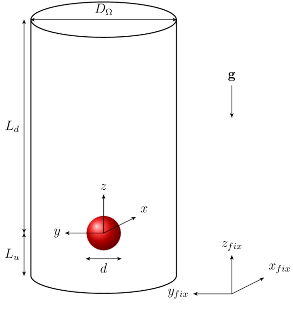
Figure 1: The geometry of the problem and the computational domain as employed in the reference method described in § 2.

$\displaystyle\frac{\rho_{p}}{\rho_{f}}$

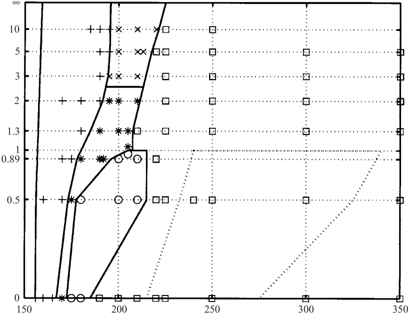
$G$

Figure 2: Diagram of flow regimes in the $(G,\rho_{p}/\rho_{f})$ parameter plane (Jenny et al., 2004). To the left of the leftmost line the wake is axisymmetric and the particle trajectory is steady and vertical. The different symbols correspond to simulations classified as: $+$, steady oblique path; $\ast$, oscillating oblique path with low frequency; $\times$, oscillating oblique path with high frequency; $\circ$, periodic zigzagging trajectory; $\Box$, three-dimensional chaotic trajectory. The dotted line delimits the region of coexistence of a chaotic and a periodic zigzagging state. The parameter values considered in the present work all lie on a horizontal line at $\rho_{p}/\rho_{f}=1.5$.

Concerning flows with significant relative velocities between the solid and the fluid phase (e.g. due to buoyancy effects as in sedimentation systems), our personal experience has shown that the above array of validation tests might not be representative of all relevant flow features. In particular, the subtle dynamics of particle motion due to differences in wake characteristics in the various regions of the parameter space may not be sufficiently captured by a numerical code at a given resolution although it might perform reasonably well in the above cases. Therefore, the purpose of the present work is to provide a further benchmark configuration serving as a test of simulation tools for fully-resolved fluid-particle motion.

The case of a single settling unconfined sphere in the absence of solid boundaries appears an attractive configuration in this context. On one hand, high-fidelity data can be generated by means of relatively efficient reference simulations with spectral accuracy (Jenny and Dušek, 2004). In the reference method, the mesh is translated with the immersed object which avoids remeshing (Mougin and Magnaudet, 2002). On the other hand, as mentioned above, the settling process of a single sphere covers all the essential dynamics involved in general sedimentation problems, including very subtle effects of wake-induced non-trivial trajectories, while excluding additional complexity due to inter-particle collisions. It is as such a challenging and rigorous test case for any non-geometry-conforming numerical simulation method. At the same time the benchmark simulations need not be excessively demanding, since the size of the computational domain can be kept relatively small. Furthermore, the initial state and the boundary conditions of the problem are simple and well-defined.

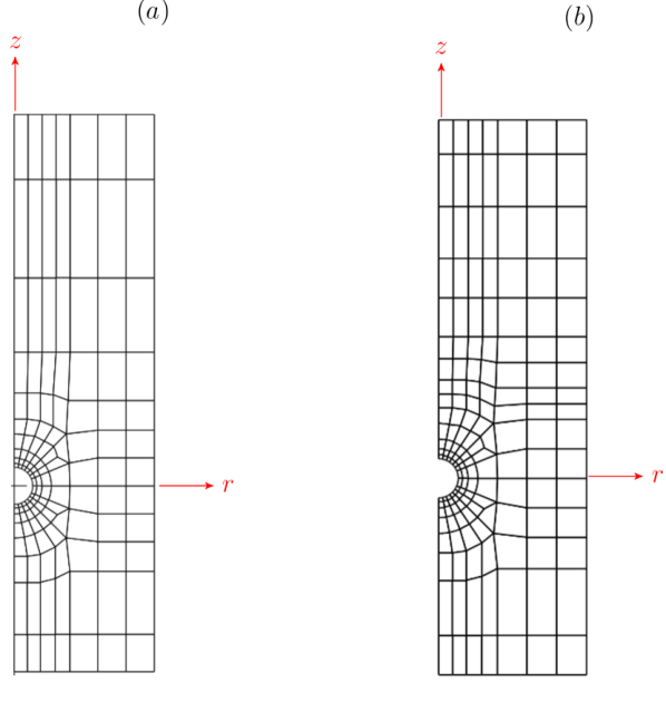
Figure 3: The spectral element meshes used in the axial/radial plane of the coordinate system attached to the particle in cases with lateral domain size $D_{\Omega}=7.54$: $(a)$ mesh with 134 elements, used for simulations with $G=\{144,178.46\}$; $(b)$ mesh with 169 elements, used for $G=\{190,250\}$.

For this purpose we have generated detailed data for the flow field and the rigid body motion in the case of a single heavy sphere settling in quiescent surroundings, using a highly accurate spectral/spectral-element method. The simulations are similar to those performed by and described in Jenny et al. (2004). However, in the present work the computational domain was purposefully kept small, thereby requiring new simulations. Furthermore, in the present paper we aim at reporting a complete set of data (contrary to the previous publication of Jenny et al., 2004) for the purpose of validating alternative numerical methods.

In parallel, we report results from computations of the same flow configuration obtained by means of a non-geometry-conforming code based upon an immersed boundary method (IBM, Uhlmann, 2005a). We have performed refinement tests from which the required small-scale resolution can be deduced in each flow regime.

The outline of the paper is the following. In § 2 the flow geometry, boundary conditions and the numerical method used to generate the reference data is described, before we proceed to present the benchmark data. In § 3 we further illustrate the validation procedure by describing simulations performed with an immersed boundary method; the numerical approach is first summarized (§ 3.1) and then the results are compared to the reference data (§ 3.2). The paper closes with a summary and discussion in § 4.

2 Reference case

2.1 Flow configuration and governing equations

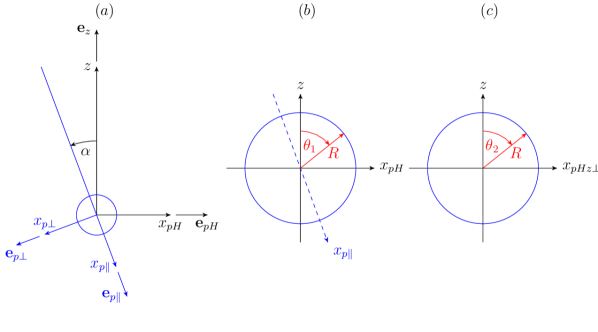
Figure 4: $(a)$ Sketch of the notation concerning directional unit vectors and coordinates in the plane spanned by the vertical axis $\mathbf{e}_{z}$ and the direction of the particle motion $\mathbf{e}_{p\parallel}$, as defined in § 2.4.1. Note that the direction $\mathbf{e}_{pHz\perp}$ is perpendicular to the plane of the sketch which corresponds to the plane defined by the trajectory and the vertical direction. The axes $\mathbf{e}_{pH}$, $\mathbf{e}_{pHz\perp}$ and $\mathbf{e}_{z}$ (as well as $\mathbf{e}_{p\perp}$, $\mathbf{e}_{pHz\perp}$, $\mathbf{e}_{p\parallel}$) form a right-handed coordinate system. $(b,c)$ Definition of two great circles on the sphere (located in two planes which are perpendicular to each other), as used for the presentation of the pressure coefficient below. These graphs define the angles $\theta_{1}$ and $\theta_{2}$ along the great circles.

We are considering the motion of a spherical solid body with diameter $d$ immersed in a fluid under the action of a gravitational field. Figure 1 illustrates the geometry of the problem as well as the definition of the different coordinate systems which will be used in the following. The first set of Cartesian coordinates $(x,y,z)$ describes a position with respect to the center of the sphere. Secondly, the Cartesian coordinates with respect to a fixed origin are denoted as $(x_{fix},y_{fix},z_{fix})$. The directions of the axes in both of these Cartesian coordinate systems are the same, with the $z$ and $z_{fix}$ axes pointing into the direction opposite to gravity. The position of the sphere in the fixed coordinate system is henceforth denoted as $\mathbf{x}_{sphere}$. Alternatively, we use a cylindrical coordinate system (the origin of which is attached to the center of the particle), with the coordinates denoted as $(z,r,\theta)$, $r$ being the radial coordinate and $\theta$ the azimuthal angle in the horizontal plane.

The equations for the flow of a viscous incompressible fluid can be written as

$$\partial_{t}\mathbf{u}+\left(\left[\mathbf{u}-\mathbf{u}_{p}\right]\cdot\nabla\right)\mathbf{u}+\nabla p = \frac{1}{G}\nabla^{2}\mathbf{u}\,,$$ (1a)

$$\nabla\cdot\mathbf{u} = 0\,.$$ (1b)

In (1) the fluid velocity vector with respect to the fixed frame is denoted by $\mathbf{u}$, $\mathbf{u}_{p}$ is the sphere’s translational velocity vector in the fixed frame (with components $u_{p},v_{p},w_{p}$), and $p$ is the hydrodynamic pressure without the hydrostatic part. The equations given in (1) have been made dimensionless by means of the reference scales $\ell_{ref}=d$, $u_{ref}=(a_{ref}\ell_{ref})^{1/2}$, $t_{ref}=\ell_{ref}/u_{ref}$ and $p_{ref}=\rho_{f}u_{ref}^{2}$ for length, velocity, time and pressure, respectively. In doing so, the characteristic acceleration $a_{ref}=|\rho_{p}/\rho_{f}-1|g$ has been used, where $\rho_{f}$ is the fluid density, $\rho_{p}$ the sphere’s density and $g$ the magnitude of the vector of gravitational acceleration, i.e. $g=|\mathbf{g}|$. The dimensionless parameter $G$ appearing in the Navier-Stokes equations (1) under this choice of reference scales is the Galileo number defined as:

$$G=\frac{\sqrt{\left|\frac{\rho_{p}}{\rho_{f}}-1\right|\,g\,d^{3}}}{\nu}\,.$$ (2)

Note that the Galileo number is equivalent to a Reynolds number defined with the sphere diameter as the length scale and the gravitational velocity $u_{ref}=(|\rho_{p}/\rho_{f}-1|gd)^{1/2}$ as the velocity scale. At a point on the sphere surface ${\cal S}$, the no-slip boundary condition accounting for the sphere translation and rotation reads:

$$\mathbf{u}|_{\cal S}=\mathbf{u}_{p}\,+\,\boldsymbol{\omega}_{p}\times\mathbf{r}_{\cal S}\,,$$ (3)

where $\boldsymbol{\omega}_{p}$ is the angular velocity vector describing the rotation of the sphere with respect to its center and $\mathbf{r}_{\cal S}$ the position vector at the sphere surface with respect to the center.

The motion of the immersed solid sphere is described by the following equations

$$\frac{\rho_{p}}{\rho_{f}}\frac{\mbox{d}\mathbf{u}_{p}}{\mbox{d}t} = \frac{6}{\pi}\oint_{\cal S}\left(\boldsymbol{\tau}\cdot\mathbf{n}-p\mathbf{n}\right)\,\mbox{d}S-\mathbf{i}\,,$$ (4a)

$$\frac{\rho_{p}}{\rho_{f}}\frac{\mbox{d}\boldsymbol{\omega}_{p}}{\mbox{d}t} = \frac{60}{\pi}\oint_{\cal S}\mathbf{r}_{S}\times\left(\boldsymbol{\tau}\cdot\mathbf{n}\right)\,\mbox{d}S\,,$$ (4b)

where the same reference quantities as in (1) have been used. In (4) the angular velocity vector $\boldsymbol{\omega}_{p}$ has components $\omega_{px},\omega_{py},\omega_{pz}$, $\boldsymbol{\tau}$ is the viscous stress tensor whose components are given by $\tau_{ij}=(\partial u_{i}/\partial x_{j}+\partial u_{j}/\partial x_{i})/G$, $\mathbf{n}$ denotes the outward pointing unit vector normal to the surface ${\cal S}$ of the sphere and $\mathbf{i}$ is the unit vector pointing in the vertical direction.

The coupled system of field equations for the fluid flow (1) and ordinary differential equations for the sphere motion (4) is fully characterized by two non-dimensional numbers, namely the Galileo number $G$ (as defined in 2) and the density ratio $\rho_{p}/\rho_{f}$. Note that for steady motion of the sphere the value of the density ratio is not relevant any more and the problem is fully determined by the value of the Galileo number. Figure 2 gives an overview of the features exhibited by the motion of an immersed sphere in the parameter space spanned by the values of $G$ and $\rho_{p}/\rho_{f}$ (Jenny et al., 2004). It will be further discussed in § 2.3 below.

2.2 Numerical method

case	$\rho_{p}/\rho_{f}$	$G$	$D_{\Omega}$
AS	$1.5$	$144$	$5.34$
AL	$1.5$	$144$	$7.54$
BS	$1.5$	$178.46$	$5.34$
BL	$1.5$	$178.46$	$7.54$
CS	$1.5$	$190$	$5.34$
CL	$1.5$	$190$	$7.54$
DS	$1.5$	$250$	$5.34$
DL	$1.5$	$250$	$7.54$

Table 1: Parameter points in the $(G,\rho_{p}/\rho_{f})$ plane and diameter $D_{\Omega}$ of the cylindrical domain in the present reference simulations. In the descriptive name of each case (first column), “S” refers to the smaller domain with $D_{\Omega}=5.34$ and “L” to $D_{\Omega}=7.54$.

The numerical method used as the basis for the present development has been described in Ghidersa and Dušek (2000) and Jenny and Dušek (2004). The spatial discretization takes advantage of the axisymmetry of the computational domain for expanding the variables into a rapidly converging azimuthal Fourier series. The so obtained azimuthal Fourier modes are functions of only the radial distance $r$ and of the axial projection $z$. They obey a set of two-dimensional equations coupled via the advective terms. The discretization in the radial–axial plane $(r,z)$ uses the spectral element decomposition (Patera, 1984). The time discretization is chosen in view of solving high Reynolds number flows. In this case the adopted time splitting approach, used already in Patera (1984), is both accurate and efficient. The non-linear terms are treated explicitly (in our case we use the third order Adams-Bashforth method), which un-couples linear two-dimensional Stokes-like problems in individual azimuthal subspaces numbered by the azimuthal wavenumber $m$. The latter are solved by splitting the pressure–velocity coupling into a Poisson pressure equation and a Helmholtz equation for the velocity. In the literature (e.g. Karniadakis et al., 1991), the splitting is considered before the discretization. Kotouč et al. (2008) have noted that, if the whole augmented matrix of the Stokes–like problem is created, the matrix obtained by multiplying the discretized divergence by the discretized gradient is not exactly the same as that of the diffusion operator. The so obtained improvement of accuracy was combined with a considerable reduction of computational costs achieved by replacing the iterative (conjugate gradient) pressure solver by a direct method.

At the inflow (bottom) cylinder basis the velocity is set equal to zero to simulate an asymptotically quiescent fluid. At the outflow (top) cylinder basis and at its side a no stress Neumann boundary condition is imposed on the velocity field and a zero pressure is set.

In the present simulations we have employed grids with different numbers of spectral elements: for the small domain size, the radial/axial plane was tesselated with 129 elements; for the tesselation of the larger domain size 134 elements were used at the lower Galileo number values ($G=144$ and $G=178$), while 169 elements were used at $G=190$ and $G=250$. Figure 3 shows these grids.

In all cases 6 collocation points in each of the two spatial directions internal to each element were used. Furthermore, the azimuthal Fourier expansion was truncated above mode 7. Finally, the time step has been adjusted such that the CFL number takes a value of 0.25. Extensive validation and grid convergence studies (Jenny and Dušek, 2004; Bouchet et al., 2006) have demonstrated the adequacy of this spatial and temporal resolution in the present parameter range.

2.3 Overview of sphere dynamics and flow regimes

The state diagram in figure 2 features 5 different symbols corresponding to the following classification.

case	$u_{pV}$	$L_{r}$	$Re_{\parallel}$
AS	$-1.292$	$1.385$	$186.05$
AL	$-1.285$	$1.383$	$185.08$

Table 2: Reference results for flow cases in the steady axi-symmetrical flow regime ($G=144$).

For Galileo numbers below a value of approximately 155 (at all density ratios, cf. also Fabre et al., 2012), steady vertical particle motion with full axisymmetry in the horizontal plane is obtained. When increasing the Galileo number beyond the threshold of that primary bifurcation, the axisymmetry of the wake is broken, and a regime with steady oblique particle motion exists. Further increasing the Galileo number for a given density ratio, a Hopf bifurcation occurs, leading to oscillating oblique paths; the diagram in figure 2 actually shows two such oscillating oblique regimes, distiguished by the value of the oscillation frequency, roughly occurring for $\rho_{p}/\rho_{f}$ above or below a value of 2.5. For density ratios smaller than unity (i.e. rising spheres) the oblique oscillating state was found to give way to a ‘zig-zagging’ state (marked by open circles in figure 2), i.e. to a rise along a periodic and wavy trajectory remaining vertical in the mean. The frequency was shown to be about three times smaller than that of the low frequency oblique oscillating state. For $\rho_{p}/\rho_{f}>1$ (for falling spheres) the oblique oscillating state becomes directly chaotic when further increasing the Galileo number. Conversely, for rising spheres intermittent chaos was shown to arise from the zig-zagging state. The chaotic states are all marked by the same symbol in figure 2, although there are significant qualitative differences between highly intermittent states close to the right limit (upper limit in terms of the Galileo number) of the stability of the periodic zig-zagging state and much less ordered states at high Galileo numbers and high density ratios. In view of subsequent experimental observations (Veldhuis and Biesheuvel, 2007; Horowitz and Williamson, 2010), the region delimited (roughly) by the dotted line in figure 2 is especially noteworthy. It corresponds to the region of bi-stability between chaotic and periodic states. The periodic states are, again, vertical in the mean (zig-zagging), however, their frequency is significantly higher than that of the states marked by open circles. The frequency is close to that evidenced in Veldhuis and Biesheuvel (2007) and Horowitz and Williamson (2010) for experimental zig-zagging trajectories. The low-frequency zig-zagging state has never been observed experimentally, very likely because of its weak stability (Jenny et al., 2004).

2.4 Reference data

$(a)$

$(b)$

$z$

$(c)$

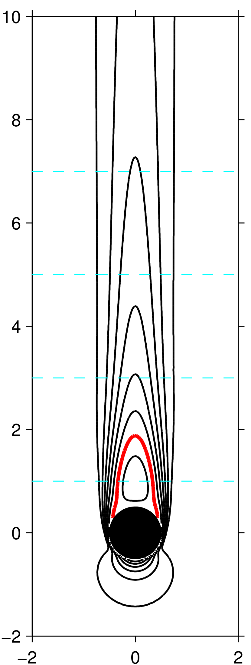
$r$

Figure 5: Reference results for case AL ($G=144$). $(a)$ The surface where the vertical relative velocity $u_{r\parallel}=1.2$ (corresponding to $0.93|u_{pV}|$). $(b)$ The surface where $\lambda_{2}=-0.015$ (cf. definition in the text). $(c)$ Contours of the vertical relative velocity $u_{r\parallel}$ in the vertical/radial plane passing through the particle center. Contours are shown for values (-0.2:0.2:1.2); the red line marks the extent of the recirculation region (i.e. $u_{r\parallel}=0$). The cyan colored dashed lines indicate the positions of the velocity profiles which are given in the supplementary data and which are compared to the IBM results in figure 20.

With the purpose of providing data for validation and benchmarking of numerical simulation codes, we have selected a set of parameter points which are representative of the different regimes of sphere motion. With the aim of keeping the data-set tractable, we have considered a single density ratio which was chosen as $\rho_{p}/\rho_{f}=1.5$. This value corresponds to particles with a moderately higher density than the fluid (e.g. polyester in water). Concerning the Galileo number, four values were considered such that each case corresponds to one of the observed regimes of motion of falling spheres:

• $G=144$: steady vertical fall, axi-symmetric wake (case A);

• $G=178$: steady oblique fall, double-threaded wake (case B);

• $G=190$: oscillating oblique fall (case C);

• $G=250$: chaotic motion (case D).

Therefore, the chosen parameter points sample a cross-section of the parameter map shown in figure 2 at $\rho_{p}/\rho_{f}=1.5$. With increasing $G$ these parameter points represent a sequence of flow cases with increasing physical complexity and – due to the onset of unsteadiness and further bifurcations – of increasing demand from the point of view of a numerical method.

In the present work we have strived to use a relatively small computational domain in order to maintain the computational effort in subsequent studies, where successive refinement will be performed, manageable. As a consequence, we have chosen two values for the horizontal diameter of the cylindrical domain, $D_{\Omega}=\{5.34,7.54\}$, cf. sketch in figure 1, while maintaining the vertical length fixed at $L_{x}=15$ (with $L_{u}=5$ and $L_{d}=10$ the vertical length upstream and downstream of the particle center, respectively). All reference simulations were run in both, the wider and the smaller cylindrical domains. As a side effect, the sensitivity of the results with respect to the domain size can be gauged.

Please refer to table 1 for a summary of the parameter values which have been simulated in the present work. The table also shows the two-letter abbreviations which will be used in the following when referring to the respective flow cases: the first letter denotes the flow regime (from A to D), the second one designates the lateral domain size (S or L, i.e. “small” or “large”).

$y$

$(a)$

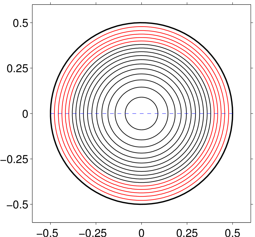
$x$

$(b)$

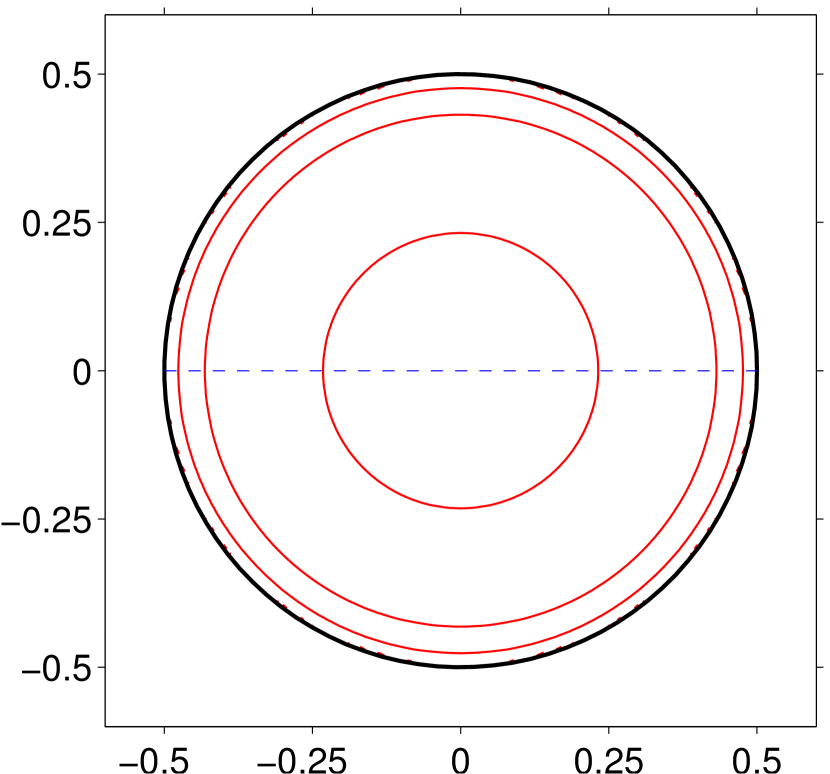
$x$

Figure 6: Reference results for case AL showing the pressure coefficient $c_{p}$. $(a)$ Contours of $c_{p}$ on the surface of the sphere, projected upon the horizontal plane through the sphere’s center (upstream-facing side). Contours are shown for values (-0.5:0.1:1.1), with negative values being indicated by red color. $(b)$ The same as $(a)$, but for the downstream-facing side of the sphere.

2.4.1 Geometric definitions and notation

Let us first fix the notation used in the subsequent presentation of flow and particle data. The particle velocity relative to the ambient fluid velocity $\mathbf{u}_{\infty}$ is defined as

$$\mathbf{u}_{pr}=\mathbf{u}_{p}-\mathbf{u}_{\infty}\,,$$ (5)

with Cartesian components $\mathbf{u}_{pr}=(u_{pr},v_{pr},w_{pr})^{T}$. Note that throughout § 2.4 we have $\mathbf{u}_{\infty}=0$. The Reynolds number based upon the magnitude of the relative particle velocity is simply obtained as follows

$$Re_{\parallel}=\frac{|\mathbf{u}_{pr}|\,u_{ref}\,d}{\nu}=|\mathbf{u}_{pr}|\,G\,.$$ (6)

Its values will be listed in the tables below for convenience.

case	$u_{pV}$	$u_{pH}$	$\omega_{pH}$	$L_{r}$	$Re_{\parallel}$
BS	$-1.363$	$0.1270$	$0.0136$	$1.631$	$244.29$
BL	$-1.356$	$0.1245$	$0.0137$	$1.629$	$243.01$

Table 3: Reference results for flow cases in the steady oblique flow regime ($G=178.46$).

$(a)$

$(b)$

$(c)$

$(d)$

Figure 7: Reference results for case BL ($G=178.46$). Graphs $(a)$ and $(b)$ show the surface where $u_{r\parallel}=1.2$ (corresponding to $0.88|\mathbf{u}_{pr}|$), Graphs $(c)$ and $(d)$ show the surface where $\lambda_{2}=-0.015$ (cf. definition in the text). In $(a)$ and $(c)$ the view is directed along $\mathbf{e}_{pHz\perp}$; in $(b)$ and $(d)$ it is directed along $\mathbf{e}_{pH}$.

The magnitude of the particle velocity (relative to the ambient) in the horizontal plane is denoted as $u_{pH}$, defined through

$$u_{pH}=\sqrt{u_{pr}^{2}+v_{pr}^{2}}\,.$$ (7)

The vertical component of the particle velocity relative to the ambient fluid velocity is given by

$$u_{pV}=w_{pr}\,.$$ (8)

$z$

$(a)$

${x}_{pH}$

$x_{p\parallel}$

$(b)$

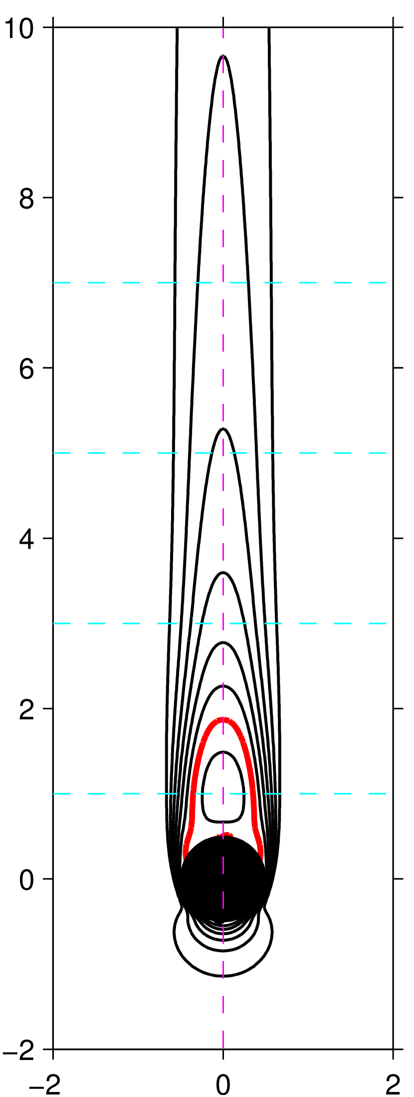
${x}_{pHz\perp}$

Figure 8: Reference results for case BL ($G=178.46$). $(a)$ Contours of the projected relative velocity $u_{r\,\parallel}$ in the plane which is spanned by the vertical direction $\mathbf{e}_{z}$ and the direction of the particle motion $\mathbf{e}_{p\parallel}$, passing through the sphere’s center. Contours are shown for values (-0.4:0.2:1.2); the red line marks the extent of the recirculation region (i.e. $u_{r\,\parallel}=0$). The blue cross marks the location which defines the recirculation length $L_{r}$. The magenta colored dashed line indicates the direction of the particle motion given by the unit vector $\mathbf{e}_{p\,\parallel}$. $(b)$ Same as $(a)$, but in the plane spanned by $\mathbf{e}_{pHz\perp}$ and $\mathbf{e}_{p\parallel}$, passing through the sphere’s center. The cyan colored dashed lines in $(a)$ and $(b)$ indicate the positions of the velocity profiles which are given in the supplementary data and which are compared to the IBM results in figure 25.

The horizontal ($\omega_{pH}$) and vertical components ($\omega_{pV}$) of the angular particle velocity are similarly defined as

$$\omega_{pH} = \sqrt{\omega_{px}^{2}+\omega_{py}^{2}}\,,$$ (9a)

$$\omega_{pV} = \omega_{pz}\,.$$ (9b)

The directional unit vector $\mathbf{e}_{pH}$ of the particle motion in the horizontal plane (in cases of non-vertical motion, $u_{pH}>0$) is given by

$$\mathbf{e}_{pH}=\left(u_{pr},v_{pr},0\right)^{T}/u_{pH}\,.$$ (10)

The component of the position vector in the direction $\mathbf{e}_{pH}$ (measured from the sphere’s center) will be denoted by $x_{pH}$; the direction perpendicular to $\mathbf{e}_{pH}$ in the horizontal plane (i.e. also perpendicular to $\mathbf{e}_{z}$) is referred to as

$$\mathbf{e}_{pHz\perp}=\left(-v_{pr},u_{pr},0\right)^{T}/u_{pH}\,,$$ (11)

(with associated coordinate $x_{pHz\perp}$) in the following. In the case of purely vertical motion (corresponding to purely axi-symmetric flow), the definitions (10) and (11) do not apply; cylindrical coordinates $(z,r,\theta)$ will be chosen instead, as defined in § 2.1.

$x_{pH}$

$(a)$

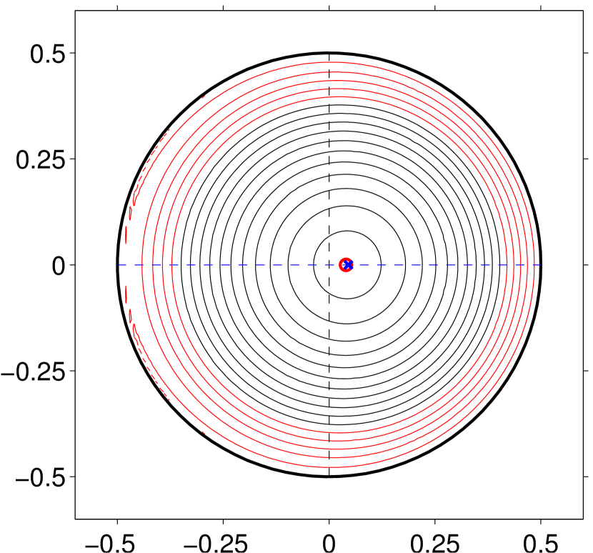
$x_{pHz\perp}$

$(b)$

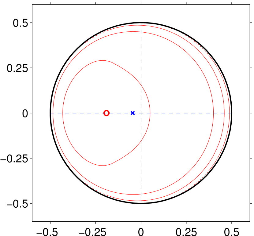
$x_{pHz\perp}$

Figure 9: Reference results for case BL showing the pressure coefficient $c_{p}$. $(a)$ Contours of $c_{p}$ on the surface of the sphere, projected upon the horizontal plane through the sphere’s center (upstream-facing side). Contours are shown for values (-0.5:0.1:1.1), with negative values being indicated by red color. The blue cross marks the point where the axis of motion, $\mathbf{e}_{p\parallel}$, crosses the sphere’s surface. The red circle marks the location of the local pressure maximum on the depicted hemisphere. $(b)$ The same as $(a)$, but for the downstream-facing side of the sphere.

The fluid velocity field expressed in the coordinate system attached to the particles (i.e. the fluid velocity relative to the particle motion) is defined as

$$\mathbf{u}_{r}(\mathbf{x},t)=\mathbf{u}(\mathbf{x},t)-\mathbf{u}_{p}(t)\,,$$ (12)

with Cartesian components $\mathbf{u}_{r}=(u_{r},v_{r},w_{r})^{T}$. The unit vector pointing in the direction of the particle motion relative to the ambient is defined as

$$\mathbf{e}_{p\,\parallel}=\mathbf{u}_{pr}/||\mathbf{u}_{pr}||\,,$$ (13)

and the distance from the sphere’s center along this direction is denoted by $x_{p\,\parallel}$. The direction which is perpendicular to both $\mathbf{e}_{pHz\perp}$ and $\mathbf{e}_{p\,\parallel}$ is given by

$$\mathbf{e}_{p\,\perp}=\mathbf{e}_{pHz\perp}\times\mathbf{e}_{p\,\parallel}\,,$$ (14)

again with corresponding coordinate $x_{p\,\perp}$. A sketch of these geometrical definitions in the plane given by the vertical coordinate direction and the particle velocity vector is shown in figure 4.

The relative fluid velocity projected upon the direction opposite to the particle velocity vector (relative to the ambient) is given by

$$u_{r\,\parallel}=\mathbf{u}_{r}\cdot\left(-\mathbf{e}_{p\,\parallel}\right)\,,$$ (15)

(note the negative sign), and the components in the two remaining coordinate directions of the frame ($\mathbf{e}_{p\perp}$,$\mathbf{e}_{pHz\perp}$,$\mathbf{e}_{p\parallel}$) are denoted as:

$$u_{r\,\perp} = \mathbf{u}_{r}\cdot\mathbf{e}_{p\perp}\,,$$ (16a)

$$u_{r\,Hz\perp} = \mathbf{u}_{r}\cdot\mathbf{e}_{pHz\perp}\,.$$ (16b)

The quantity $u_{r\,\parallel}$ is used for the definition of the sphere wake recirculation length which is determined as follows. Let us define a curve ${\cal C}$ as the connection of locations where the projected relative velocity $u_{r\,\parallel}$ changes sign in a plane passing through the sphere center and which is parallel to both the vertical direction $\mathbf{e}_{z}$ and the direction of the sphere’s translational velocity $\mathbf{e}_{p\,\parallel}$. Then the recirculation length $L_{r}$ is measured as the largest distance between the sphere’s surface and any point on the curve ${\cal C}$. A graphical impression of our definitions of the recirculation length can be gathered from figure 8 which will be discussed in § 2.4.3. With the present notation, the pressure coefficient can be defined as follows:

$$c_{p}=\frac{p-p_{\infty}}{|\mathbf{u}_{pr}|^{2}/2}\,,$$ (17)

where $p_{\infty}$ is the pressure of the ambient fluid, and the relative particle velocity $\mathbf{u}_{pr}$ is defined in (5). Note that the fluid density is absent in the denominator of (17) due to the choice of reference quantities (cf. § 2.1).

2.4.2 Steady axi-symmetric regime

case	$\overline{u}_{pV}$	$\overline{u}_{pH}$	$\overline{\omega}_{pH}$	$u_{pV}^{\prime}$	$u_{pH}^{\prime}$	$\omega_{pH}^{\prime}$	$f$	$\overline{L}_{r}$	${L}_{r}^{\prime}$	$Re_{\parallel}$
CS	$-1.383$	$0.137$	$0.013$	$0.010$	$0.040$	$0.010$	$0.068$	–	–	$264.06$
CL	$-1.376$	$0.136$	$0.012$	$0.008$	$0.033$	$0.008$	$0.071$	$1.681$	$0.069$	$262.71$

Table 4: Reference results for flow cases in the oscillating oblique flow regime ($G=190$). Overbars stand for mean values and primes for fluctuation amplitudes, as defined in (19-20). The Reynolds number $Re_{\parallel}$ (defined in 6) is computed from the mean velocity values.

$u_{pV}$

$(a)$

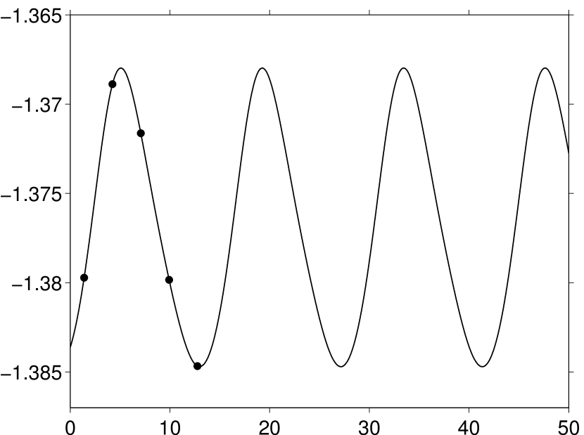
$t$

$u_{pH}$

$(b)$

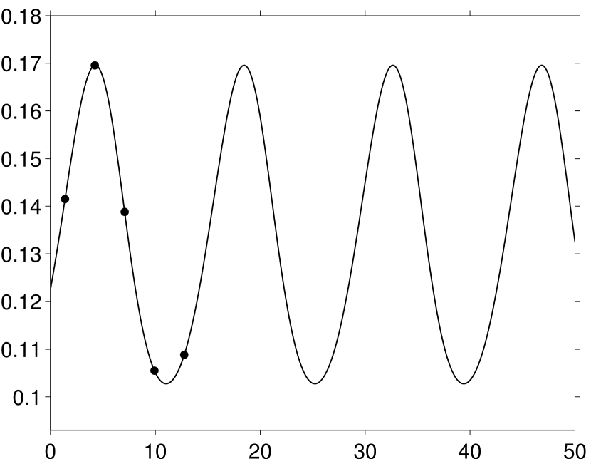
$t$

Figure 10: Reference results for case CL ($G=190$), exhibiting time-periodic dynamics. The graphs show the temporal evolution of: $(a)$ the vertical particle velocity component; $(b)$ the horizontal particle velocity component. The symbols indicate the time instants corresponding to the flow fields shown in figures 11 and 12.

When the Galileo number is set to $G=144$ the particle wake under fully established conditions is axi-symmetric, the particle motion is steady and it follows a straight vertical path. Therefore, the angular particle velocity is identically zero, and its translational velocity only has one non-zero component, $u_{pV}$. Table 2 lists the asymptotic, steady-state values of $u_{pV}$ obtained for the two domain sizes which have been simulated. It can be seen that the difference is small (approximately $0.5$%), which implies that a variation of the domain size in the present range ($D_{\Omega}=5.34$ to $7.54$) has an almost negligible influence on the particle motion.

Figure 5 gives a visual impression of the flow field around the particle in steady-state motion for case AL. The graph in figure 5$(a)$ shows an iso-surface of the vertical component of the flow velocity relative to the particle motion. It can be seen that after approximately one diameter downstream of the rear stagnation point, the wake is almost aligned with the vertical direction. Also included in the figure is an iso-surface plot of the second largest eigenvalue of the tensor $\mathbf{S}^{2}+\boldsymbol{\Omega}^{2}$ (where $\mathbf{S}$ and $\boldsymbol{\Omega}$ are the symmetrical and anti-symmetrical parts of the velocity gradient tensor, respectively), henceforth denoted as $\lambda_{2}$. It has been proposed by Jeong and Hussain (1995) that vortical structures can be identified with regions where the quantity $\lambda_{2}$ takes negative values. Figure 5$(b)$ shows that vortical motion in the present case is concentrated in a thin torus-shaped region enclosing the sphere.

Contours of the fluid velocity relative to the particle motion, $u_{r\parallel}$ (cf. definition in equ. 15), are shown in figure 5$(c)$. The extent of the region where $u_{r\parallel}<0$ is marked in red therein. The length of this recirculation region is given in table 2. Again, it can be seen that the influence of the lateral domain size is almost negligible (less than $0.2$%). The vertical component of the relative fluid velocity along the vertical axis through the sphere’s center (i.e. along a vertical cut through figure 5$c$) exhibits the expected rapid deceleration when approaching the front stagnation point, takes negative values in the recirculation region, and has a slower recovery (proportional to the inverse of the distance from the downstream stagnation point) further downstream along the axis. This information is included in the supplementary data and it is compared to the IBM results in figure 20 below. Furthermore, radial profiles of the two non-zero velocity components in the cylindrical coordinate system attached to the particle center (the axial component $u_{r\parallel}$ and the radial component, henceforth denoted as $u_{rad}$) at four different axial locations: $x_{p\parallel}=\{-1,-3,-5,-7\}$ (along the dashed lines marked in figure 5$c$) are provided in the supplementary data.

$(a)$

$(b)$

$(c)$

$(d)$

$(e)$

$(f)$

$(g)$

$(h)$

$(i)$

$(j)$

Figure 11: Reference results for case CL ($G=190$, time-periodic dynamics), showing instantaneous flow fields, with time increasing from left to right by increments of $T/5$ ($T$ being the period). The surface where $\lambda_{2}=-0.005$ (cf. definition in the text) is visualized. In $(a$-$e)$ the view is directed along $\mathbf{e}_{pHz\perp}$; in $(f$-$j)$ it is directed along $\mathbf{e}_{pH}$.

Finally, in figure 6 we report data for the pressure on the sphere’s surface. Contours of the pressure coefficient $c_{p}$ (cf. definition in 17) projected upon a horizontal plane (on the upstream and downstream sides of the sphere) are presented. From the different density of contour-lines along the radial direction it can be inferred that the pressure gradients are much larger on the upstream side as compared to the downstream side, clearly showing the incomplete pressure recovery in the recirculation zone. The values of the pressure coefficient along a great circle are included in the supplementary material; they will be compared to the IBM data in figure 21 below.

2.4.3 Steady oblique regime

$z$

$(a)$

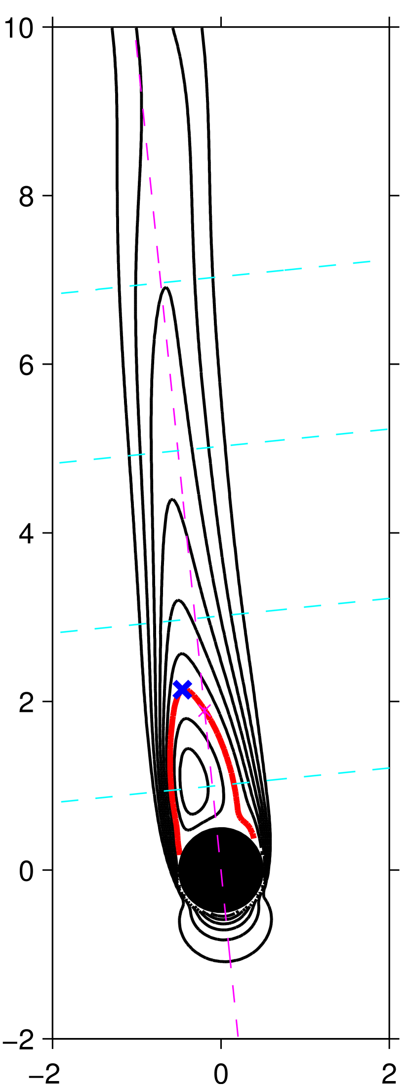
${x}_{pH}$

$(b)$

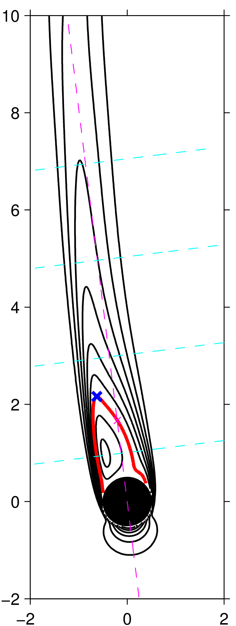
${x}_{pH}$

$(c)$

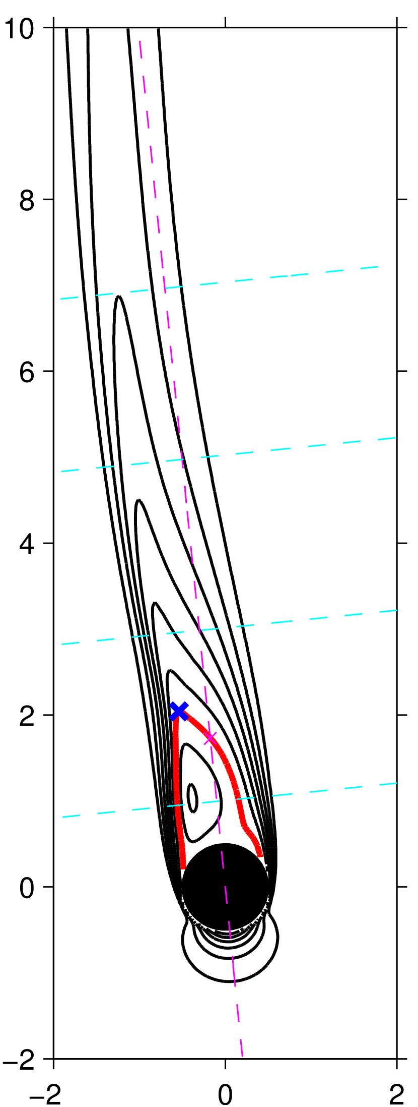
${x}_{pH}$

$(d)$

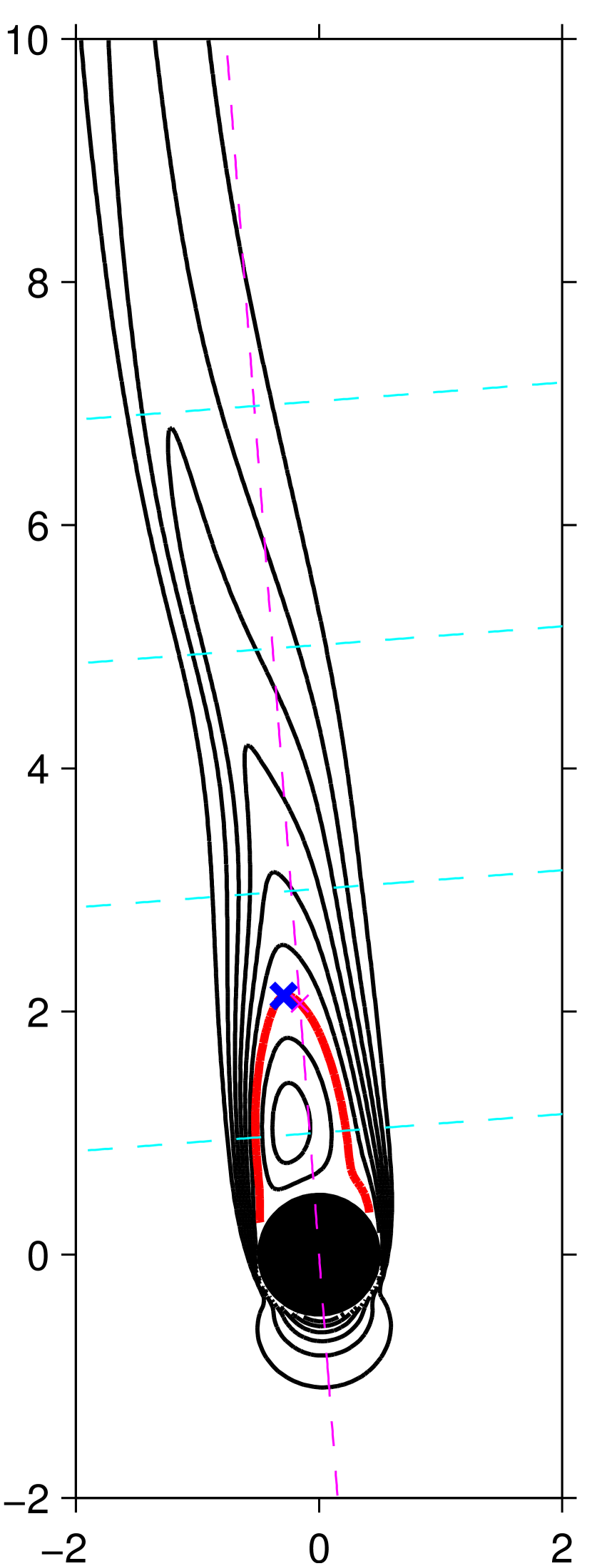
${x}_{pH}$

$(e)$

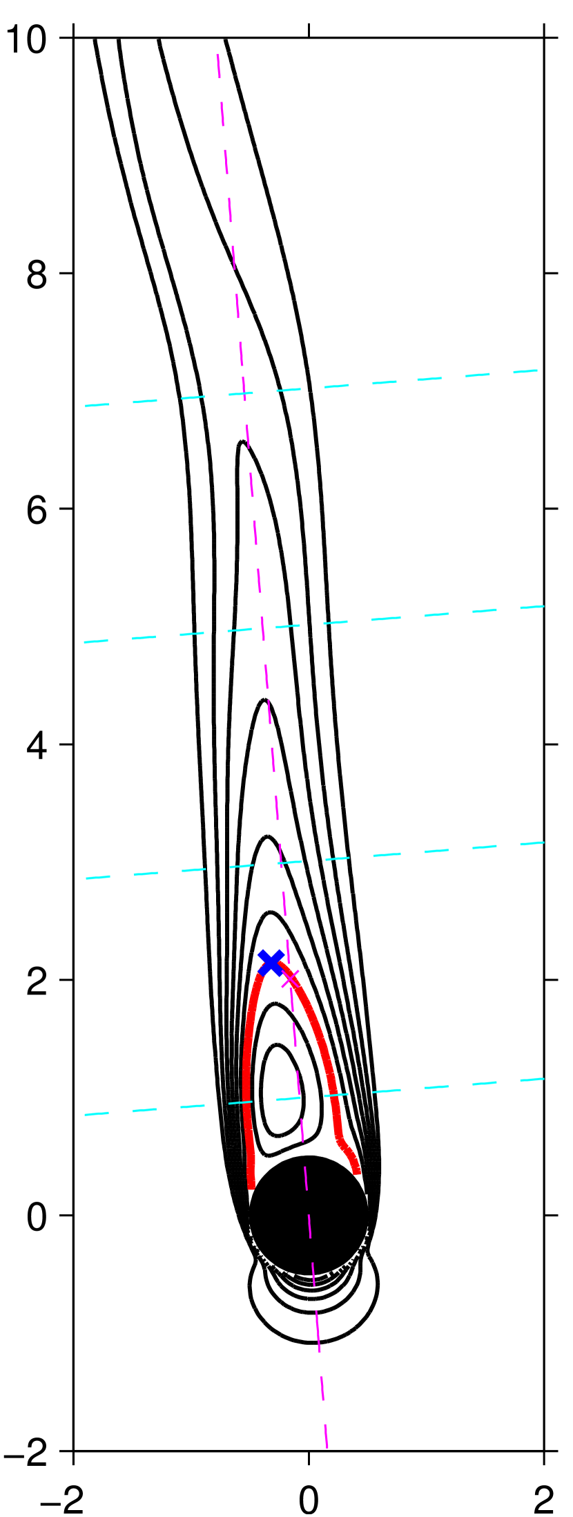
${x}_{pH}$

$x_{p\parallel}$

$(f)$

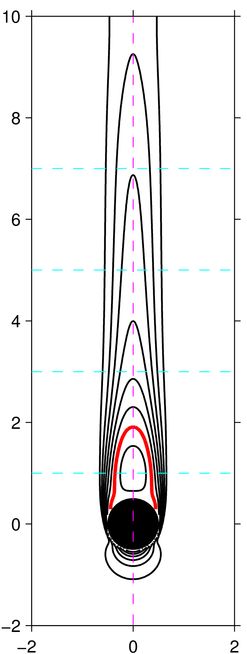
${x}_{pHz\perp}$

$(g)$

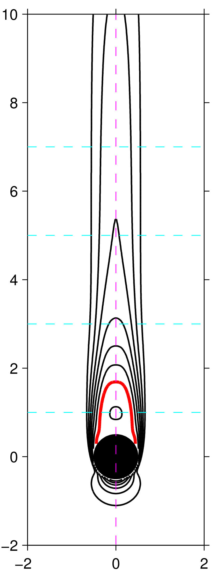
${x}_{pHz\perp}$

$(h)$

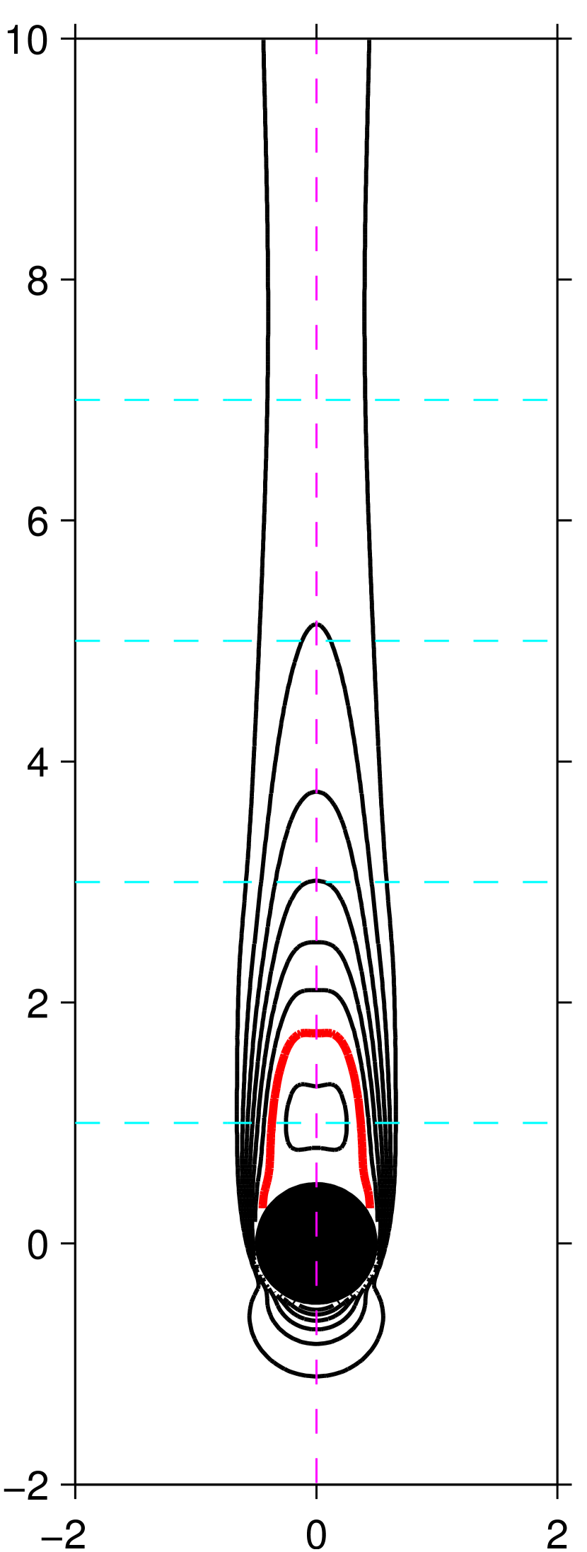
${x}_{pHz\perp}$

$(i)$

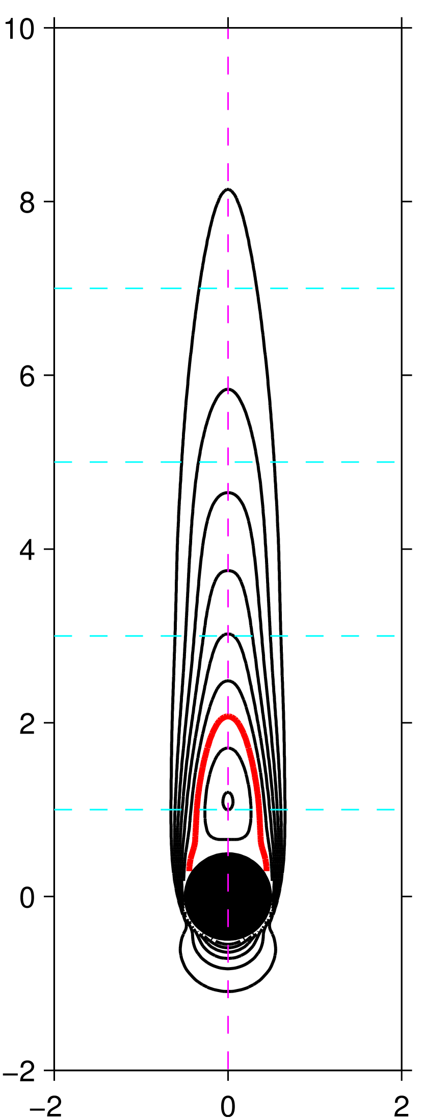
${x}_{pHz\perp}$

$(j)$

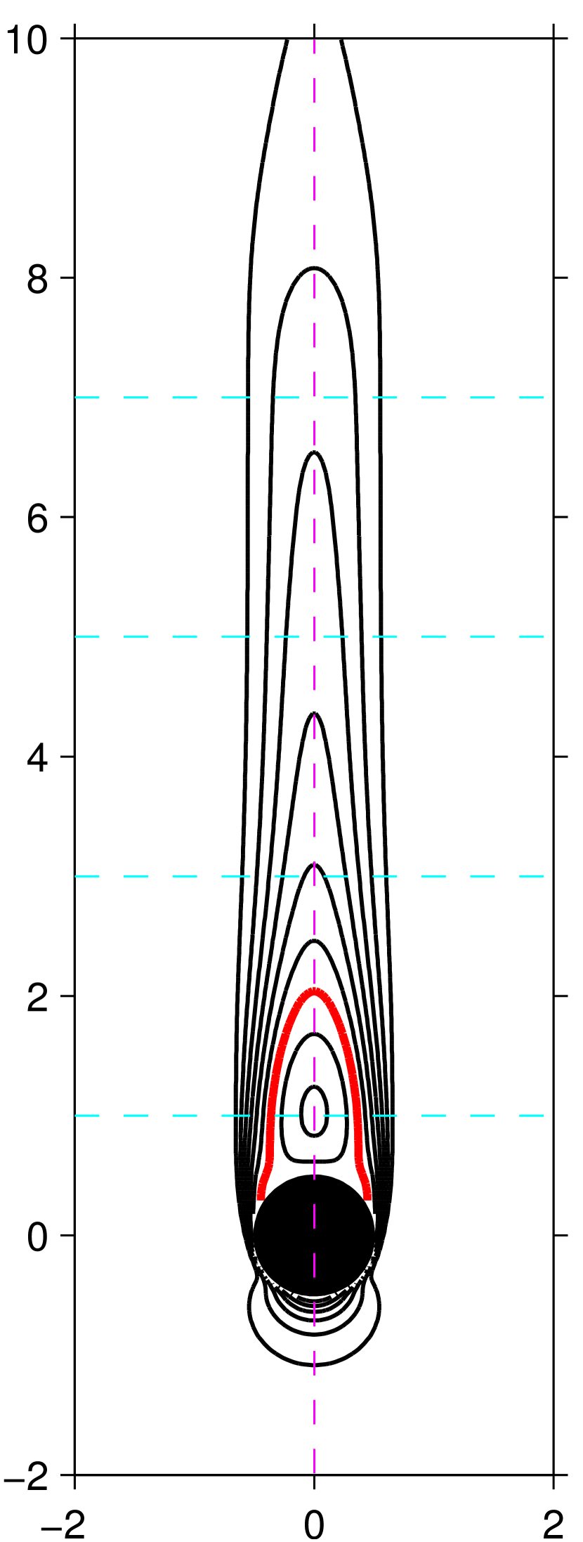
${x}_{pHz\perp}$

Figure 12: As figure 11, but showing contours of the projected relative velocity $u_{r\,\parallel}$. In $(a$-$e)$ a plane spanned by the vertical direction $\mathbf{e}_{z}$ and the direction of the particle motion $\mathbf{e}_{p\parallel}$, passing through the sphere’s center, is chosen. In $(f$-$j)$ the plane spanned by $\mathbf{e}_{pHz\perp}$ and $\mathbf{e}_{p\parallel}$, passing through the sphere’s center, is chosen. The red line marks the instantaneous extent of the recirculation region (i.e. $u_{r\,\parallel}=0$). The magenta colored dashed line indicates the direction of the particle motion given by the unit vector $\mathbf{e}_{p\,\parallel}$.

In the second regime, here simulated with a Galileo value of $G=178.46$, the particle wake (in the fully developed state) is no longer axi-symmetric, but still steady. Therefore, the particle motion is along a non-vertical straight path. Consequently, in addition to the vertical particle velocity component, $u_{pV}$, the horizontal one ($u_{pH}$, along unit vector $\mathbf{e}_{pH}$) is non-zero; furthermore, the particle rotates with angular velocity $\omega_{pH}$ around the horizontal axis $\mathbf{e}_{pHz\perp}$ (i.e. perpendicular to $\mathbf{e}_{pH}$). Table 3 lists the numerical values obtained in our simulations for both domain sizes. Again, it is found that the influence of the domain size is very small. An interesting parameter is the angle of particle motion with respect to the vertical, whose tangent is given by the ratio of horizontal to vertical amplitude, viz.

$$\tan(\alpha)=\frac{u_{pH}}{|u_{pV}|}\,.$$ (18)

The values for the angle $\alpha$ are $5.323$ and $5.225$ degrees for case BS and BL, respectively.

Figure 7 provides an impression of the flow field around the sphere in case BL, showing iso-surfaces of the relative velocity $u_{r\parallel}$ and of $\lambda_{2}$ as seen from two different angles. In particular, the iso-surface plot of $\lambda_{2}$ reveals the double-threaded structure of the wake, with both threads lying slightly off-center, therefore generating a horizontal force component upon the sphere. This observation is confirmed in figure 8$(a,b)$, where contours of the relative velocity (projected upon the direction opposite to the sphere’s velocity relative to the ambient fluid) are shown in two perpendicular planes. The maximum extent of the recirculation region is found off center (i.e. the recirculation length $L_{r}$ is larger than $L_{r\parallel}$, cf. table 3). The relative fluid velocity $u_{r\parallel}$ along the axis defined by the particle velocity (i.e. along $\mathbf{e}_{p\parallel}$ through the sphere’s center) is included in the supplementary data-set; it will also be used in the comparison with the IBM data below (cf. figure 23 and 24).

$w_{pr}$

$(a)$

$t$

$u_{pr}$

$(b)$

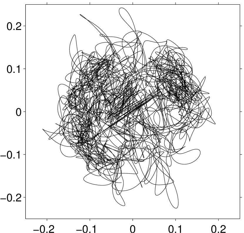
$v_{pr}$

Figure 13: Reference results for case DL ($G=250$), exhibiting chaotic dynamics. $(a)$ Temporal evolution of the vertical particle velocity component (measured relative to the ambient fluid velocity). $(b)$ Phase-space plot in the two-dimensional space spanned by the two horizontal particle velocity components.

Note that relative velocity profiles along the directions $\mathbf{e}_{pHz\perp}$ (at $x_{p\perp}=0$) and along $\mathbf{e}_{p\perp}$ (at $x_{pHz\perp}=0$) at various distances $x_{p\parallel}=\{-1,-3,-5,-7\}$ downstream of the rear stagnation point are included in the supplementary data-set. This information is used in the comparison with the IBM data in figure 25 below.

The surface pressure data for case BL is visualized in figure 9. The contours projected upon the horizontal plane are roughly similar to the axi-symmetric case (cf. figure 6). However, the pressure maximum on the upstream side is now shifted towards a small positive value of $x_{pHz\perp}$ (approximately coinciding with the point where the axis of motion crosses the sphere’s surface, cf. blue cross in figure 9$a$). Contrarily, on the downstream side – due to the non-axi-symmetric wake – the local pressure maximum considerably moves off center (red circle in figure 9$b$), much more than the inclination of the sphere’s axis of motion (blue cross in figure 9$b$).

2.4.4 Oscillating oblique regime

At a value of the Galileo number of $G=190$ the asymptotic state of the particle motion is characterized by a periodic temporal evolution. Particle motion still takes place in a single plane given by the (time-independent) vectors $\mathbf{e}_{z}$ and $\mathbf{e}_{pH}$ (as in the steady oblique regime of § 2.4.3), but the quantities themselves are time-dependent. Therefore, in this regime there are three non-zero, time-dependent components of the translational and angular particle velocity, i.e. $u_{pH}(t)$, $u_{pV}(t)$ and $\omega_{pH}(t)$. As can be seen from figure 10, the signals of these quantities are similar to a single harmonic, but a closer analysis reveals that they are in fact anharmonic. Instead of providing a complete fit to a multicomponent sine base (which appears to converge only slowly), we provide simple measures of the oscillating signals as follows. The mean and the amplitude of a particle-related quantity $\phi(t)$ are defined from the maxima and minima as

$$\overline{\phi}\equiv\frac{\phi_{max}+\phi_{min}}{2}\,,$$ (19)

and

$$\phi^{\prime}\equiv\frac{\phi_{max}-\phi_{min}}{2}\,,$$ (20)

respectively. The oscillation period $T$ is determined from a count of the zero-crossings of the fluctuation values $\phi-\overline{\phi}$ over a time sufficiently larger than (i.e. several multiples of) the period. The oscillation frequency $f$ is then simply obtained as the inverse of $T$.

Table 4 lists the numerical values describing the oscillating signals. First, it is once more observed that the lateral domain size does not play a significant role, as the difference between choosing $D_{\Omega}=5.34$ and $7.54$ is below 0.5% (0.2%) of the value $u_{pV}$ in case CS for the translational (angular) velocity components. The oscillation frequency $f$ differs by approximately 4% between cases CS and CL. Secondly, it is found that the mean values for translational and angular particle velocities are similar to the steady-state values obtained at $G=178.46$. Note that the oscillation frequency is indeed small. The observed period $T$ corresponds roughly to the time during which the sphere has covered a vertical distance of 20 diameters.

The graphs in figure 11 show visualizations of the flow field in terms of iso-surfaces of $\lambda_{2}$ for five snapshots equally distributed over one oscillation cycle. It can be seen that the shape of the wake significantly varies over the oscillation period. Although the vortical structure in the near-field of the sphere still principally exhibits a double-threaded character (much alike case BL), over one oscillation period the vortex threads first grow in axial length, then detach from the sphere, whence a new double thread is formed.

A more detailed picture of the cycle is provided by the sequence of graphs of the contours of the projected relative velocity $u_{r\parallel}$ shown in figure 12. The swaying in direction $\mathbf{e}_{p\perp}$ is confirmed, while the simultaneous temporal evolution of the recirculation region can be observed (figure 12$a$-$e$). In the plane given by $\mathbf{e}_{p\parallel}$ and $\mathbf{e}_{pHz\perp}$ (figure 12$f$-$j$), on the other hand, it can be seen that the axial growth of the vortical structures in the wake first causes a stretching and thinning of the wake, and then a subsequent retraction and further growth in axial extent. In order to quantify the variation of the recirculation length $L_{r}$ over each period, we have defined an average and a fluctuation value, henceforth denoted by $\overline{L}_{r}$ and $L_{r}^{\prime}$, respectively, using the definitions given in (19) and (20), and using data from the five snapshots shown in figure 12. The values for case CL are listed in table 4. We observe that the mean recirculation length $\overline{L}_{r}$ is slightly larger than in case BL (same domain, but $G=178.46$). The amplitude of the fluctuations $L_{r}^{\prime}$ measures approximately 4% of the mean value.

Note that the surface pressure variation along two perpendicular great circles for the same sequence of snapshots is contained in the supplementary data-set (figure omitted).

2.4.5 Chaotic regime

case	$\langle{u}_{pV}\rangle$	$\langle u_{pV}^{\prime\prime}u_{pV}^{\prime\prime}\rangle^{1/2}$	$\langle u_{pr}^{\prime\prime}u_{pr}^{\prime\prime}\rangle^{1/2}$	$\langle\omega_{pV}^{\prime\prime}\omega_{pV}^{\prime\prime}\rangle^{1/2}$	$\langle\omega_{px}^{\prime\prime}\omega_{px}^{\prime\prime}\rangle^{1/2}$	$Re_{\parallel}$
DL	$-1.4604$	$0.0087$	$0.0854$	$0.0013$	$0.0067$	$365.10$

Table 5: Reference results for cases DL in the chaotic flow regime ($G=250$), accumulated over a sampling period of $2250$ time units. The Reynolds number $Re_{\parallel}$ (defined in 6) is computed from the average velocity value.

$(a)$

$(b)$

$(c)$

$(d)$

Figure 14: Reference results for case DL ($G=250$, chaotic dynamics), showing an instantaneous flow field. Graphs $(a)$ and $(b)$ show the surface where $u_{r\parallel}=1.2$ (corresponding to $0.82|\langle{u}_{pV}\rangle|$). Graphs $(c)$ and $(d)$ show the surface where $\lambda_{2}=-0.2$ (cf. definition in the text). In $(a)$ and $(c)$ the view is directed along $\mathbf{e}_{pHz\perp}$; in $(b)$ and $(d)$ it is directed along $\mathbf{e}_{pH}$. Note that some spectral-element boundaries are visible in $(c)$ and $(d)$.

$(a)$

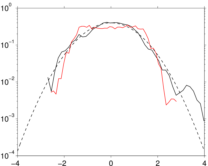
$u_{p\alpha}^{\prime\prime}/\sigma$

$\sigma\cdot pdf$

$\sigma\cdot pdf$

$(b)$

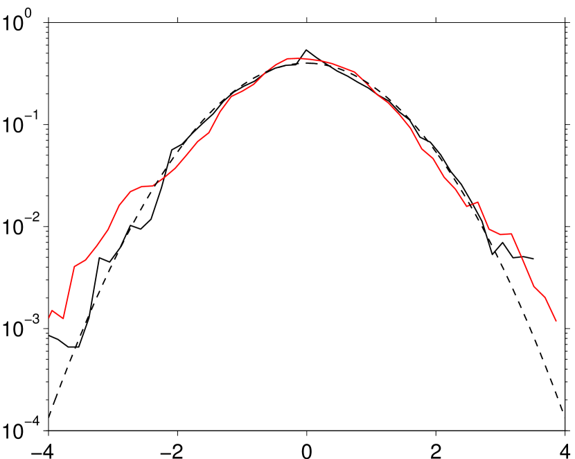
$\omega_{p\alpha}^{\prime\prime}/\sigma$

Figure 15: Reference results for case DL ($G=250$). Probability density functions of: $(a)$ translational particle velocity; $(b)$ angular particle velocity. The line-styles are as follows: ——–, vertical component; ——–, horizontal component; – – – –, Gaussian reference curve.

$(a)$

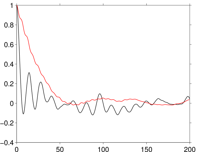
$\tau_{sep}$

$R_{u_{p\alpha}u_{p\alpha}}$

$R_{\omega_{p\alpha}\omega_{p\alpha}}$

$(b)$

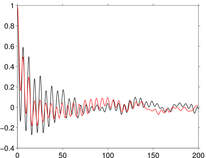
$\tau_{sep}$

Figure 16: Reference results for case DL ($G=250$). Temporal auto-correlations of: $(a)$ translational particle velocity; $(b)$ angular particle velocity. The line-styles are as follows: ——–, vertical component; ——–, horizontal component.

We have observed that the system settles into a chaotic state when the Galileo number is set to $G=250$ and the larger computational domain is used (case DL). Contrarily, in the smaller domain (case DS) the system remains in a state characterized by zig-zagging motion in a vertical plane. It is interesting to note that the zig-zagging state is that co-existing with the chaotic one and having the high, experimentally evidenced, frequency $0.147$. At this Galileo number it is slightly quasi-periodic. The chaotic and zig-zagging states do not co-exist with the considered confinements. We will henceforth concentrate upon case DL, which exhibits chaotic dynamics.

The temporal evolution of the vertical particle velocity component in case DL is shown in figure 13$(a)$, while figure 13$(b)$ depicts a phase-space diagram of the two horizontal velocity components. Substantial fluctuations of all degrees of freedom are recorded. Figure 14 shows the flow field at one instant during the chaotic particle motion in case DL (again showing iso-surfaces of the relative velocity $u_{r\parallel}$ and of $\lambda_{2}$ from two different view angles). It can be seen that in the near-field of the particle (up to approximately $4$ diameters downstream) the wake remains qualitatively similar to the above cases at lower Galileo number, still exhibiting two principal threads. However, further downstream the shape of the wake becomes considerably more bent and twisted away from the direction of the instantaneous particle motion. In particular, the vortical structure exhibits a clear hairpin-like reconnection.

In order to characterize the chaotic motion quantitatively, let us define an average value of a particle-related quantity $\phi$ which is expected to converge to the statistical average when a sufficiently large number of samples is chosen, viz.

$$\langle\phi\rangle\equiv\frac{1}{\sum_{j=1}^{N_{runs}}N_{t}(j)}\sum_{j=1}^{N_{runs}}\sum_{i=1}^{N_{t}(j)}\phi(t_{i}^{(j)})\,.$$ (21)

In (21) the number of repetitions of the “experiment” is denoted by $N_{runs}$, the number of samples taken in the $j$th “experiment” by $N_{t}(j)$, and $t_{i}^{(j)}$ is the time at which the $i$th sample is taken in the $j$th “experiment”. Note that the reference computation was only run once (i.e. $N_{runs}=1$), generating samples over an interval of approximately $2250$ time units. In the chaotic regime the only particle velocity component which has a non-zero mean is the vertical one; the mean angular particle velocity is zero. Based upon the average defined in (21), we can define an instantaneous fluctuation around the mean value, i.e.

$$\phi^{\prime\prime}(t)\equiv\phi(t)-\langle\phi\rangle\,.$$ (22)

Table 5 lists the averages and fluctuation amplitudes recorded in our simulation case DL. It can be seen that the fluctuations of the translational particle velocity in the horizontal plane are roughly a factor of ten more intense than those of the vertical component. Please note that the quantity $\langle u_{pr}^{\prime\prime}u_{pr}^{\prime\prime}\rangle^{1/2}$ measures the amplitude of the fluctuations of a velocity component along one (fixed, but arbitrary) direction in the horizontal plane, which is not the same as computing the rms of $u_{pH}$. Concerning the angular particle velocity, the ratio between a component in the horizontal plane and the vertical component roughly measures $5.2$. This result is interesting, since the large discrepancy between the components should be measurable in laboratory experiments, where it could equally serve for the purpose of validation.

Normalized probability density functions of the velocity components are shown in figure 15. It can be seen that the vertical component of the (translational) particle velocity as well as all components of the angular particle velocity are approximately Gaussian distributed. Interestingly, however, the horizontal component of the translational particle velocity exhibits a plateau in the interval $u^{\prime\prime}_{pr}/\sigma(u^{\prime\prime}_{pr})\in[-1.4,1.4]$. For values outside this interval the probability drops off sharply. This feature is due to a slow rotation of the original symmetry plane found at these Galileo number values, with a near-helical trajectory (cf.  Jenny and Dušek, 2004).

The Lagrangian auto-correlation function of a particle-related quantity $\phi(t)$ is defined as

$$R_{\phi\phi}(\tau_{sep})\equiv\frac{1}{\int_{T_{1}}^{T_{2}}\phi(t)\,\phi(t)\,\mbox{d}t}\int_{T_{1}}^{T_{2}}\phi(t)\,\phi(t+\tau_{sep})\,\mbox{d}t\,.$$ (23)

This quantity can provide the information on the temporal correlation of the signals which has not been discussed up to this point. Figure 16 shows the correlation functions for the translational and angular velocity components. Again, the data for the vertical and horizontal components of the translational particle velocity are fundamentally different. Whereas the former rapidly drops to zero (first zero-crossing at $\tau_{sep}\approx 6$), the latter decays at a much slower rate (first zero-crossing at $\tau_{sep}\approx 57$). Furthermore, the auto-correlation function of the vertical component of the translational particle velocity has a marked superposed oscillation with a period of approximately $13$ time units. This oscillating feature is discernible for as long as $150$ time units. The horizontal component, on the other hand, exhibits only very weak oscillations. Turning to the angular velocity signals, it can be observed from figure 16$(b)$ that both vertical and horizontal components show similar overall features, with a rapid decay (first zero-crossing at $\tau_{sep}\approx 2.5$ and $9$, respectively) and marked superposed oscillations with a period of approximately $6.5$ time units for both components. This latter oscillation period corresponds to the frequency characterizing the ordered zig-zagging state coexisting with chaos at lower density ratios Jenny and Dušek (2004). Note that the oscillation period of the auto-correlation of the angular particle components is half the value of the oscillation period of the auto-correlation of the vertical component of the translational particle velocity.

3 Immersed boundary computations

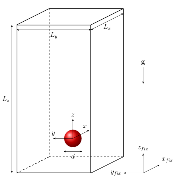
Figure 17: The computational domain as employed in the IBM computations described in § 3. The side-lengths of the cuboid were chosen as $L_{x}=L_{y}=5.34$ and $L_{z}=16$.

3.1 Numerical method

The numerical method employed in the current simulations is identical to the one presented in Uhlmann (2005a). The incompressible Navier-Stokes equations are solved by a fractional step approach with implicit treatment of the viscous terms (Crank-Nicolson) and a three-step Runge-Kutta scheme for the non-linear terms. The spatial discretization employs second-order central finite-differences on a staggered mesh; the mesh is uniform and isotropic. The no-slip condition at the surface of moving solid particles is imposed by means of a specifically designed immersed boundary technique (Uhlmann, 2005a). The motion of the particles is computed from the Newton equations for translational and angular motion of rigid bodies, driven by gravity and hydrodynamic forces/torque. The solid-fluid coupling assures that the interaction forces cancel identically when integrating over both phases.

The numerical approach has been previously validated over a wide range of flow configurations (Uhlmann, 2005a, 2006, 2007). It has been successfully employed for the simulation of various large-scale systems involving many mobile particles (Uhlmann, 2008; Uhlmann and Doychev, 2012; García-Villalba et al., 2012; Kidanemariam et al., 2013).

The immersed boundary representation of particles allows for arbitrary solid body motion with respect to the fixed computational grid. It is this feature which makes the method suitable for the simulation of many-body problems, where approaches such as the one employed in § 2 are not applicable. At the same time, the accuracy of the representation of moving particles in the framework of non-conforming methods, such as the IBM, needs to be carefully established. For this purpose, we simulate the motion of a single heavy sphere on a computational grid which is fixed in an inertial frame. Consequently, the sphere is free to move across the computational grid, and possible numerical perturbations due to the sphere’s translation are part of the errors to be gauged through the validation process.

The computational domain used in the IBM simulations is sketched in figure 17. The horizontal cross-section of the cuboid is square, with a side-length $L_{x}=L_{y}=5.34$, while the vertical length of the domain measures $L_{z}=16$. This latter dimension is slightly larger than the one used in the reference simulation of § 2. Concerning the horizontal cross-section, the smaller domain used in the reference simulations corresponds to the inscribed circle of the IBM domain, while the larger domain in that series is the circumscribed circle.

In the IBM simulations the flow velocity at the horizontal inflow plane (located at $z_{fix}=0$ in the inertial frame) is imposed, i.e.

$$\mathbf{u}(x_{fix},y_{fix},z_{fix}=0,t)=\mathbf{u}_{\infty}=(0,0,w_{\infty})\,.$$ (24)

At the horizontal outflow plane ($z_{fix}=L_{z}$) a convective outflow condition is employed (Uhlmann, 2005a). The pressure field is solved with a zero-gradient condition at the inflow and outflow planes. In both horizontal directions periodicity of the flow field over the periods $L_{x}$ and $L_{y}$, respectively, is imposed.

It should be noted that the outer geometry and boundary conditions used in the reference simulation and the IBM approach do not match in the lateral directions. However, since the reference data shows that the influence of the lateral domain size on the particle motion is rather weak (cf. tables 2-5), it is expected that the comparison is still conclusive.

The grid width $\Delta x$ has been varied in the range $D/\Delta x=15$ to $48$, as given in tables 6 to 10. This corresponds to grid sizes from $241\times 80\times 80$ up to $769\times 256\times 256$. The time step was adjusted such that the maximum CFL number was approximately $0.3$, except where stated otherwise. Henceforth, the flow cases simulated with the IBM approach are denoted with two letters (the first indicating the flow regimes A to D, the second reading “C” as in “Cartesian”) and two digits (for the number of mesh widths per sphere diameter) as in “AC-15”.

	$D/\Delta x$	$G$	$u_{pV}$	${\cal E}(u_{pV})$	$L_{r}$	${\cal E}(L_{r})$
AC-15	$15$	$144.13$	$-1.2063$	$0.0612$	$1.3431$	$0.0289$
AC-18	$18$	$144.18$	$-1.2131$	$0.0560$	$1.3688$	$0.0102$
AC-24	$24$	$143.39$	$-1.2199$	$0.0507$	$1.3785$	$0.0056$
AC-36	$36$	$142.91$	$-1.2274$	$0.0448$	$1.3835$	$0.0004$

Table 6: Results from IBM computations of case A (cf. table 1), where $\rho_{p}/\rho_{f}=1.5$ and the nominal value of the Galileo number is $G=144$. The error is computed with respect to the results of the reference case AL (cf. table 2).

$z$

$(a)$ AC-15

$r$

$(b)$ AC-18

$r$

$(c)$ AC-24

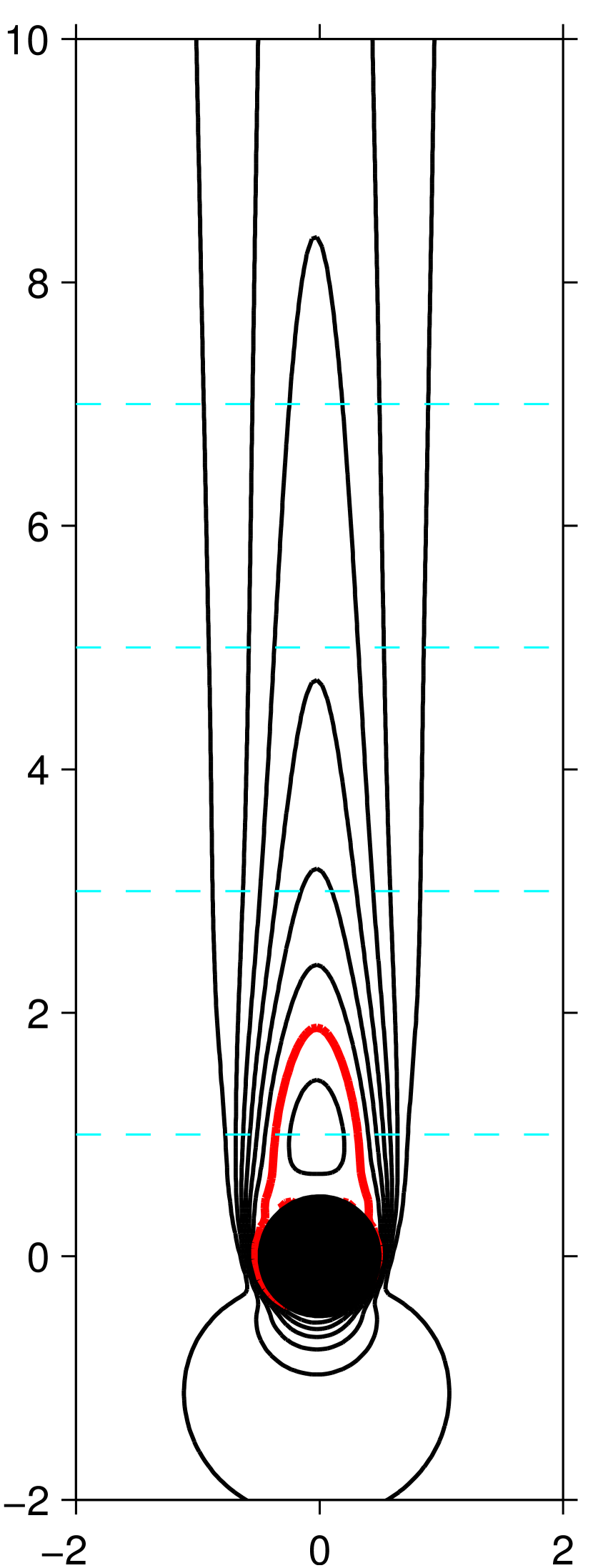
$r$

$(d)$ AC-36

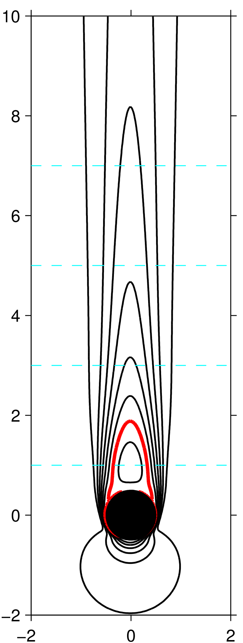
$r$

Figure 18: Data from IBM computations (at different spatial resolutions) of the steady axisymmetric case ($G=144$). The graphs show contours of the vertical relative velocity $u_{r\parallel}$ in the vertical/radial plane passing through the particle center. Contours are shown for values (-0.2:0.2:1.2); the red line marks the extent of the recirculation region (i.e. $u_{r\parallel}=0$).

The IBM simulations were initialized with a fixed particle (particle location at a distance of $5.34$ from the inflow plane), imposing a value for the Reynolds number $Re_{\infty}=|\mathbf{u}_{\infty}|D/\nu$ by adjustment of the viscosity value. After the flow around the fixed sphere was fully established, the simulation was restarted based upon the latest flow field, but now letting the sphere move freely. For the mobile case two additional parameters then need to be prescribed, namely the density ratio (which was chosen identical to the corresponding reference cases) and the value of the gravitational acceleration. In order to allow for relatively long-time integration in a fixed domain of limited extent, the buoyancy was chosen in order to approximately match the magnitude of the drag force. Therefore, the particle – once released – will not rapidly drift towards either the inflow or the outflow plane, requiring a premature termination of the simulation. In particular, the balance between drag and buoyancy yields for the value of the gravitational acceleration

$$|\mathbf{g}|=\frac{|F_{z}^{(fix)}|}{\left(\rho_{p}-\rho_{f}\right)D^{3}\pi/6}\,,$$ (25)

where $F_{z}^{(fix)}$ is the drag force acting on the particle as obtained from the fixed-particle simulation (while the values for $D$, $\nu$ and $\rho_{f}$ are kept fixed). With the value of the gravitational acceleration given by (25) the Galileo number can then be computed from its definition (2). Although the value of $G$ can be estimated, its precise magnitude is not known beforehand, therefore requiring a certain amount of experimentation in order to obtain a desired value. With the purpose of limiting the number of trials, we have allowed for small deviations with respect to the reference value of the Galileo number. This is reflected in tables 6 to 10 where the actual values are listed. It can be seen that the deviations from the nominal values are indeed small (below 1.5%).

The above described procedure does not avoid vertical drift (even in the regime where the particle motion is steady), since mobility affects the wake characteristics and, therefore, leads to modified hydrodynamic forces once the sphere is released. It simply serves the purpose of maintaining the vertical drift relatively low, thereby allowing for larger residence times of the particle inside the computational domain. Note that in all wake regimes, except for the axisymmetric one, there exists additionally a significant particle drift velocity in the horizontal plane.

$\frac{u_{r\,\parallel}}{u_{r\parallel\infty}}$

$(a)$

$z$

$(b)$

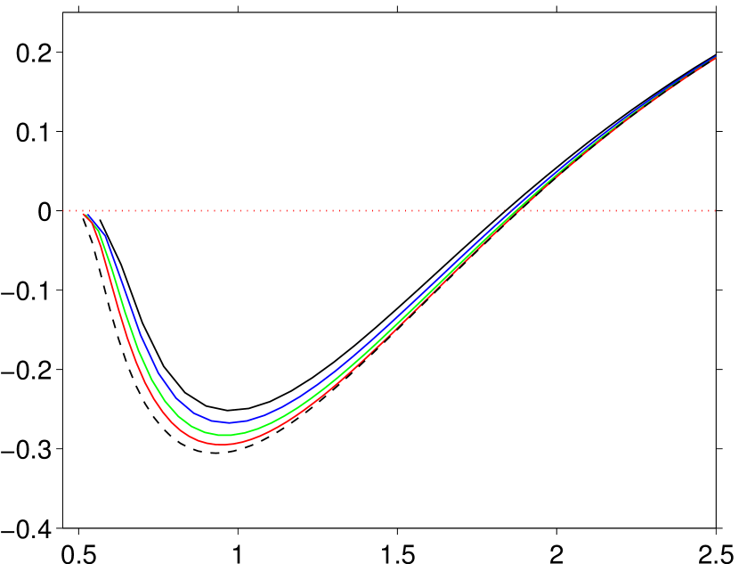
$z$

Figure 19: Data from IBM computations of the steady axisymmetric case ($G=144$), showing the quantity $u_{r\parallel}$ on the vertical axis through the particle center. The graph in $(b)$ is a close-up of the same data in the recirculation region. Line styles and color-coding indicate: ——–, case AC-15; ——–, case AC-18; ——–, case AC-24; ——–, case AC-36; – – – –, reference case AL (vertical cut through figure 5$c$).

$u_{r\,\parallel}$

$(a)$ AC-15

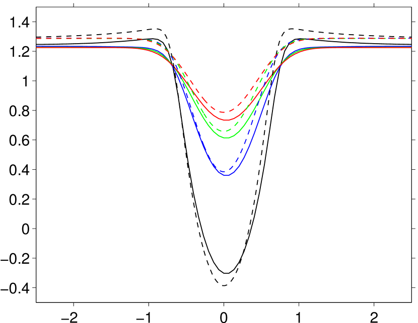
$r$

$u_{rad}$

$(b)$ AC-15

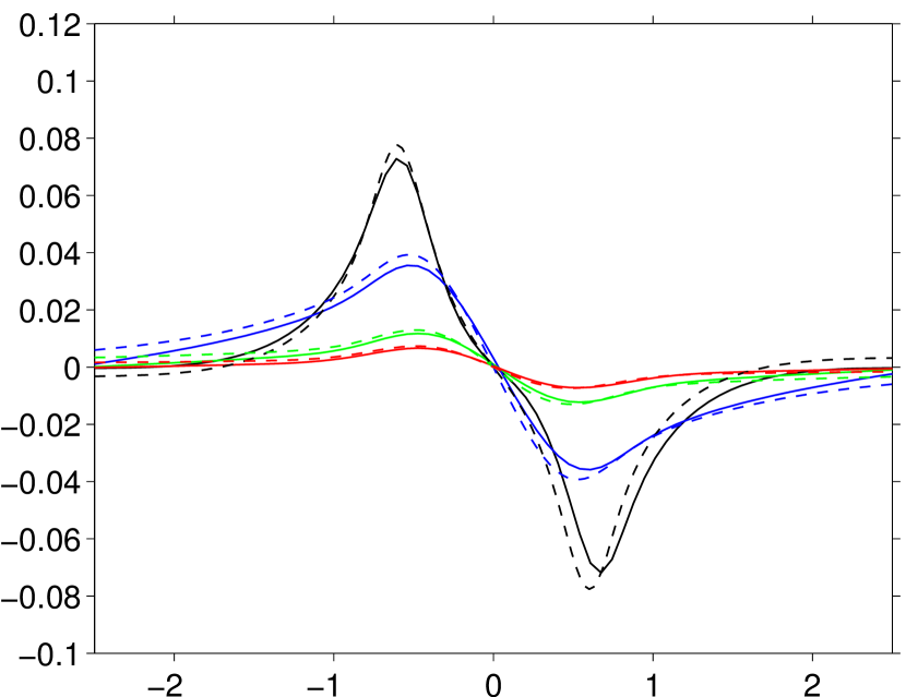
$r$

$u_{r\,\parallel}$

$(c)$ AC-36

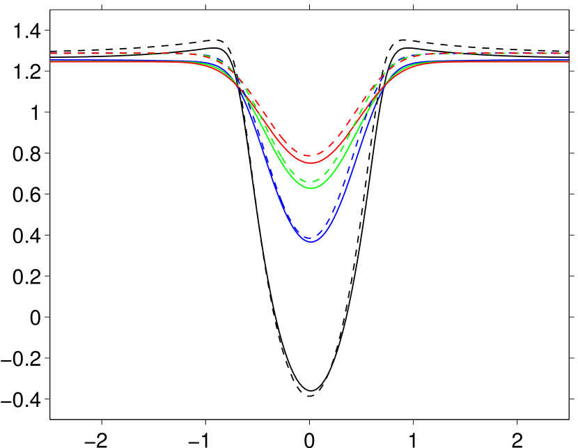
$r$

$u_{rad}$

$(d)$ AC-36

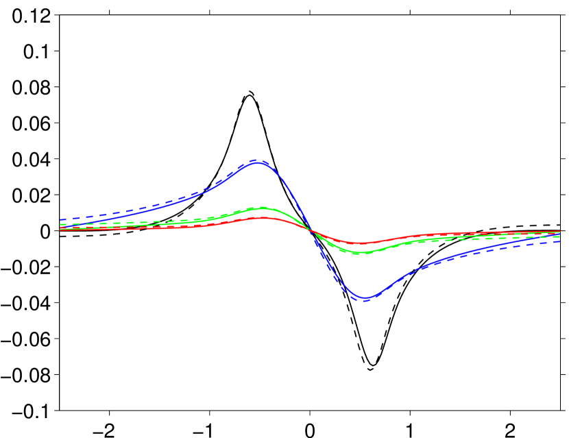
$r$

Figure 20: Radial profiles of the relative flow velocity obtained with the IBM method in case AC ($G=144$), taken along the cyan-colored dashed lines in figure 18. $(a,c)$ shows the axial velocity component $u_{r\,\parallel}$; $(b,d)$ the radial velocity component $u_{rad}$. $(a,b)$ are for case AC-15, $(c,d)$ are for case AC-36. The color code indicates the distance downstream of the sphere: ——–, $x_{p\,\parallel}=-1$; ——–, $x_{p\,\parallel}=-3$; ——–, $x_{p\,\parallel}=-5$; ——–, $x_{p\,\parallel}=-7$; the reference data (case AL) is indicated by dashed lines.

3.2 Results

$c_{p}$

$\theta$

Figure 21: Data from IBM computations of the steady axisymmetric case ($G=144$). The graph shows a profile of the pressure coefficient $c_{p}$ along a great circle on the sphere. The upstream stagnation point corresponds to a value of the angle $\theta=\pm\pi$. Please refer to figure 4 for the definition of the angle $\theta$. Line styles and symbols indicate: $\bullet$, case AC-15; $\bullet$, case AC-36; ——–, reference case AL (along blue dashed lines in figure 6).

In the following discussion we will measure the difference between a particle-related quantity $\phi$ obtained from a given simulation using the present immersed boundary method on the one hand and the reference results of § 2.4 on the other hand through a relative error ${\cal E}$ defined as

$${\cal E}(\phi)=\frac{\left|\phi-\phi^{(ref)}\right|}{\left|\phi^{(ref)}\right|}\,.$$ (26)

In the definition (26) we use the reference result $\phi^{(ref)}$ for the purpose of normalization.

At this point it should be emphasized that the present work deals with instabilities triggered by bifurcations having definite thresholds expressed by critical Galileo numbers which are very sensitive to numerical accuracy. For this reason the numerical convergence of the threshold values has been systematically used to test the numerical parameters of the spectral/spectral-element code used for generating the reference results (cf.  Ghidersa and Dušek, 2000; Jenny et al., 2004). In particular, it does not make sense to normalize relative errors by quantities becoming non-zero at instability thresholds while investigating a parameter domain in which the instabilities set in. In some instances it would amount to dividing by zero. For this reason all relative errors of non-dimensional quantities are normalized by the non-dimensional vertical velocity, i.e. we use the reference value of the vertical component, $u_{pV}^{ref}$, for computing the error of $u_{pH}$ and $\omega_{pH}$ in the denominator of (26).

The reference data used for the present comparison is taken from the results presented in § 2.4, as obtained in the larger domain with $D_{\Omega}=7.54$, i.e. cases AL, BL, CL, DL (cf. tables 1–5).

3.2.1 Steady axi-symmetric regime

$(a)$

$(b)$

$z$

$(c)$

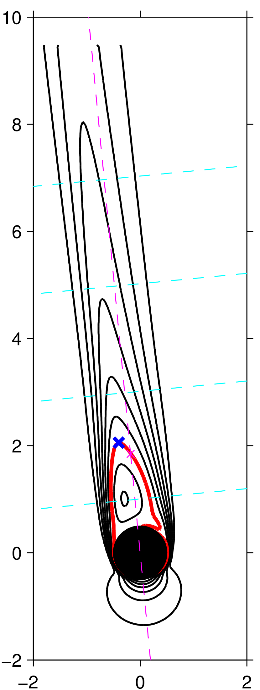
${x}_{pH}$

$z$

$(d)$

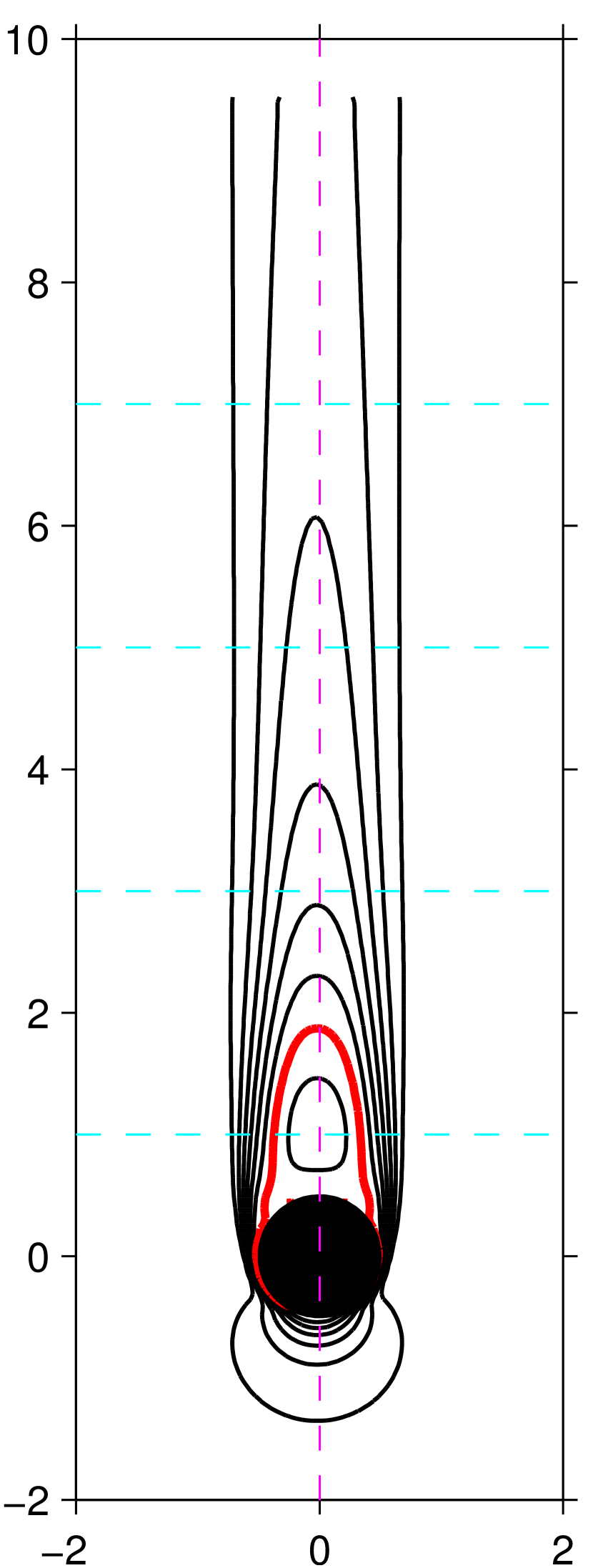
${x}_{pHz\perp}$

Figure 22: Results from IBM computation in case BC-24 ($G=178.46$). $(a)$, $(b)$ shows the surface where $\lambda_{2}=-0.015$. $(c)$, $(d)$ depict contours of the projected relative velocity $u_{r\,\parallel}$ in the plane which is spanned by the vertical direction $\mathbf{e}_{z}$ and the direction of the particle motion $\mathbf{e}_{p\parallel}$, passing through the sphere’s center. Contours are shown for values (-0.4:0.2:1.2); the red line marks the extent of the recirculation region (i.e. $u_{r\,\parallel}=0$). The blue cross in $(c)$ marks the location which defines the recirculation length $L_{r}$. The magenta colored dashed line indicates the direction of the particle motion given by the unit vector $\mathbf{e}_{p\,\parallel}$. In $(a)$ and $(c)$ the view is directed along $\mathbf{e}_{pHz\perp}$; in $(b)$ and $(d)$ it is directed along $\mathbf{e}_{pH}$.

Table 6 shows the steady-state results for the particle motion obtained with four different spatial resolutions, ranging from $D/\Delta x=15$ to $36$. It can be seen that the vertical particle velocity relative to the ambient fluid, $u_{pV}$, is slightly over-predicted by the present immersed boundary method, with the error decreasing from approximately 6% at $D/\Delta x=15$ to 4.5% at $D/\Delta x=36$. The particle wake obtained by the IBM simulation at these spatial resolutions is illustrated in figure 18 which shows contours of the vertical component of the relative flow velocity $u_{r\parallel}$ at the same levels chosen in figure 5$(c)$ for the reference case. The visual impression is that of a very good match, with the wake spreading slightly over-predicted at the lower spatial resolutions. Figure 19 shows profiles of $u_{r\parallel}$ on the vertical axis passing through the sphere’s center, allowing for a direct comparison with the reference results. Noticeable discrepancies are only found in the recirculation region. The close-up in figure 19$(b)$ illustrates the convergence towards the reference case results with increasing spatial resolution. This comparison can be made quantitative by considering the prediction of the recirculation length, $L_{r}$, the error of which is given in table 6. It is found that the relative error decreases from approximately 3% at $D/\Delta x=15$ to 0.04% at $D/\Delta x=36$.

Radial profiles of the two non-zero components of the relative flow velocity $\mathbf{u}_{r}$ in this axisymmetric case are shown in figure 20 for the two spatial resolutions $D/\Delta x=15$ and 36. The comparison with the reference results demonstrates the quality of the predictions and the convergence with increasing spatial resolution. Note that the residual difference in $u_{r\parallel}$ at large radial distances from the sphere directly reflects the respective difference in the obtained settling velocity (cf. table 6).

Finally, the pressure coefficient $c_{p}$ along a great circle (as defined in figure 4$b$) is shown in figure 21. Note that the IBM simulation (in the finite-difference context) yields values of the pressure field at the nodes of the global grid which are by definition not conforming to the spherical particle surface. Therefore, the surface pressure is not defined without ambiguity. In practice we have taken the approach of Uhlmann (2005a), plotting the pressure at the first grid node (along each grid line in one direction in the plane of the chosen great circle) outside the range of the discrete delta function, i.e. for which $|\mathbf{x}_{ijk}-\mathbf{x}_{sphere}|\geq D/2+3\Delta x/2$. The comparison in figure 21 shows that the general agreement is good even at a resolution of $D/\Delta x=15$, with the largest discrepancies occurring around the upstream stagnation point. At a spatial resolution of $D/\Delta x=36$ the match with the reference data from the spectral element method can be described as excellent.

3.2.2 Steady oblique regime

$\frac{u_{r\,\parallel}}{u_{r\parallel\infty}}$

$(a)$

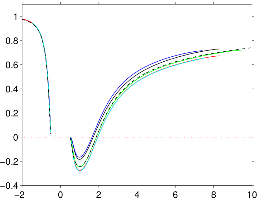
$x_{p\,\parallel}$

$(b)$

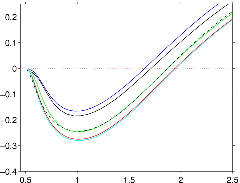
$x_{p\,\parallel}$

Figure 23: Data from IBM computations (at different spatial resolutions) of the steady oblique case ($G=178.46$), showing the quantity $u_{r\parallel}$ along the axis passing through the particle center and following the direction of the particle motion (along the magenta-colored dashed line in figure 22$c,d$). The graph in $(b)$ is a close-up of the same data in the recirculation region. Line styles and color-coding indicate: ——–, case BC-15; ——–, case BC-18; ——–, case BC-24; ——–, case BC-36; ——–, case BC-48; – – – –, reference case BL (cf. figure 8).

$\frac{u_{r\,\parallel}}{u_{r\parallel\infty}}$

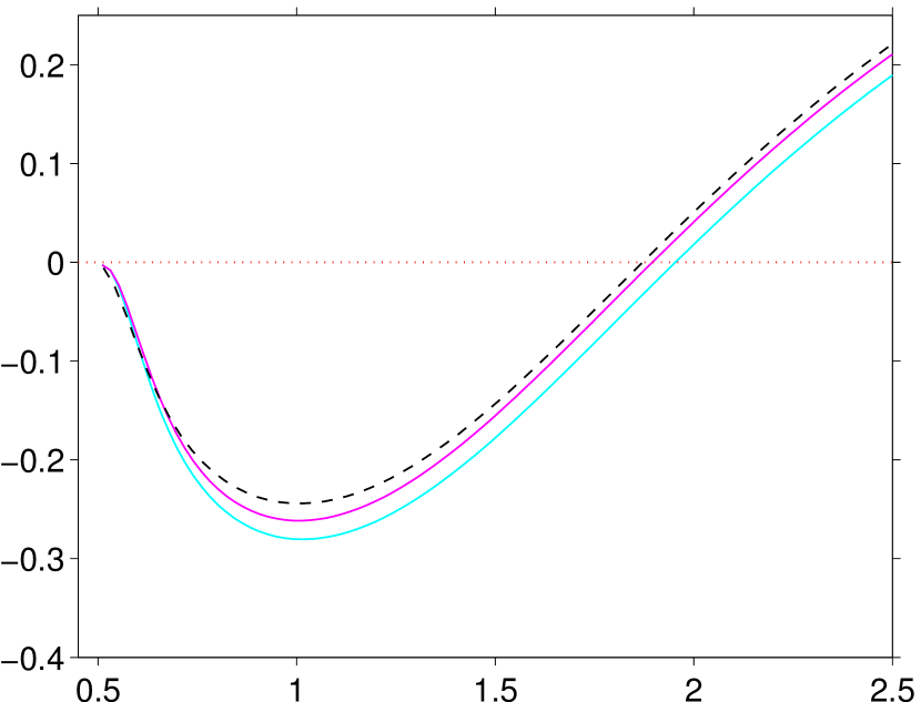
$x_{p\,\parallel}$

Figure 24: As figure 23$(b)$, comparing the IBM result with spatial resolution $D/\Delta x=48$ for two different time steps. Line styles and color-coding indicate: ——–, case BC-48 ($CFL=0.3$); ——–, case BC-48h ($CFL=0.15$); – – – –, reference case BL (cf. figure 8).

The simulations with the present immersed boundary method capture the oblique particle motion at a (nominal) Galileo number of $G=178.46$ at all chosen grid resolutions $D/\Delta x=15$ to $48$. Figure 22$(a,b)$ shows an iso-surface of $\lambda_{2}$ for case B1C-24, visualizing the same value as for the reference case in figure 7. It can be observed that the double-threaded wake structure and its inclination with respect to the vertical axis is faithfully reproduced. The same observation holds for the contours of the parallel component of the relative flow velocity, $u_{r\parallel}$, shown in figure 22$(c,d)$ which should be compared to the reference result depicted in figure 8$(a,b)$.

Profiles of the projected relative velocity $u_{r\parallel}$ along an axis parallel to $\mathbf{e}_{p\parallel}$ through the sphere’s center are shown in figure 23. It can be seen that the match with the reference data is good, with some discrepancies downstream of the particle. At this point it should be mentioned that the profiles taken along the chosen axis $\mathbf{e}_{p\parallel}$ are highly sensitive to small changes in the location of the double-threaded vortices in the wake which are attached to the particle off-center, cf. discussion in § 2.4.3. The close-up of the recirculation region provided in figure 23$(b)$ suggests that the predictions become better with refinement up to $D/\Delta x=24$ (where an excellent match is observed), and then – surprisingly – appear to converge to a profile which is slightly off the reference result (with virtually no further change when refining from $D/\Delta x=36$ to 48). We will return to this point shortly.

$u_{r\,\parallel}$

$(a)$

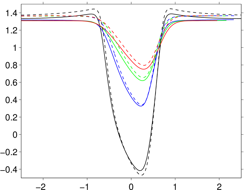
$x_{p\,\perp}$

$(b)$

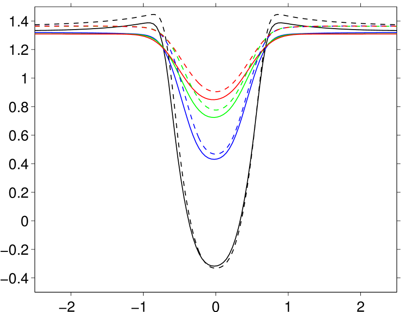
$x_{pHz\perp}$

$u_{r\,\perp}$

$(c)$

$x_{p\,\perp}$

$(d)$

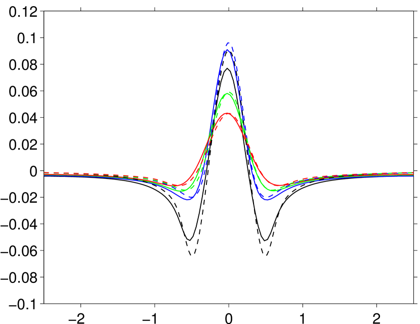
$x_{pHz\perp}$

$u_{rHz\perp}$

$(e)$

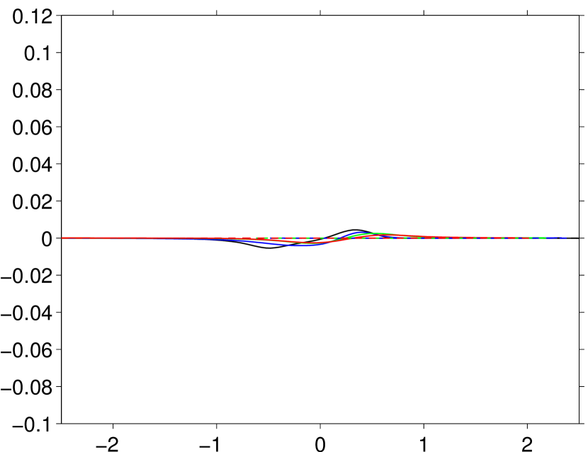
$x_{p\,\perp}$

$(f)$

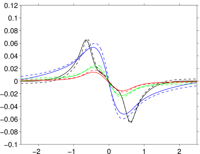
$x_{pHz\perp}$

Figure 25: Cross-profiles of the relative velocity components in local coordinates for the IBM computations in case BC-24, given along the lines indicated in cyan color in figures 8 and 22$(c,d)$. The color code indicates the distance downstream of the sphere: ——–, $x_{p\,\parallel}=-1$; ——–, $x_{p\,\parallel}=-3$; ——–, $x_{p\,\parallel}=-5$; ——–, $x_{p\,\parallel}=-7$. The reference data is shown as dashed lines with the same color code.

	$D/\Delta x$	$G$	$u_{pV}$	$u_{pH}$	$\omega_{pH}$	$L_{r}$
BC-15	$15$	$177.67$	$-1.2514$	$0.1787$	$0.0997$	$1.4983$
${\cal E}^{(BC-15)}$			$0.0771$	$0.0400$	$0.0634$	$0.0802$
BC-18	$18$	$177.42$	$-1.2695$	$0.1518$	$0.0700$	$1.5726$
${\cal E}^{(BC-18)}$			$0.0638$	$0.0201$	$0.0415$	$0.0346$
BC-24	$24$	$178.46$	$-1.2846$	$0.1242$	$0.0376$	$1.5953$
${\cal E}^{(BC-24)}$			$0.0527$	$0.0002$	$0.0176$	$0.0207$
BC-36	$36$	$176.93$	$-1.2965$	$0.1081$	$0.0162$	$1.6215$
${\cal E}^{(BC-36)}$			$0.0439$	$0.0121$	$0.0018$	$0.0046$
BC-48	$48$	$176.95$	$-1.3010$	$0.1028$	$0.0089$	$1.6291$
${\cal E}^{(BC-48)}$			$0.0406$	$0.0160$	$0.0035$	$0.0000$

Table 7: Results from IBM computations of case B (cf. table 1), where $\rho_{p}/\rho_{f}=1.5$ and the nominal value of the Galileo number is $G=178.46$. The error is computed with respect to the results of the reference case BL (cf. table 3).

	$D/\Delta x$	$G$	$u_{pV}$	$u_{pH}$	$\omega_{pH}$	$L_{r}$
BC-15h	$15$	$177.01$	$-1.2434$	$0.2090$	$0.1293$	$1.4479$
${\cal E}^{(BC-15h)}$			$0.0830$	$0.0623$	$0.0853$	$0.1112$
BC-18h	$18$	$176.72$	$-1.2668$	$0.1735$	$0.0915$	$1.5167$
${\cal E}^{(BC-18h)}$			$0.0658$	$0.0361$	$0.0574$	$0.0689$
BC-24h	$24$	$176.12$	$-1.2867$	$0.1375$	$0.0497$	$1.5665$
${\cal E}^{(BC-24h)}$			$0.0511$	$0.0096$	$0.0265$	$0.0384$
BC-36h	$36$	$176.15$	$-1.3005$	$0.1161$	$0.0236$	$1.5981$
${\cal E}^{(BC-36h)}$			$0.0409$	$0.0062$	$0.0073$	$0.0190$
BC-48h	$48$	$176.72$	$-1.3067$	$0.1110$	$0.0153$	$1.6109$
${\cal E}^{(BC-48h)}$			$0.0364$	$0.0100$	$0.0012$	$0.0107$

Table 8: As table 7, but computed with half the time step (i.e. $CFL\approx 0.15$).

$c_{p}$

$(a)$

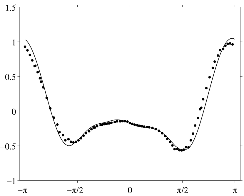
$\theta_{1}$

$(b)$

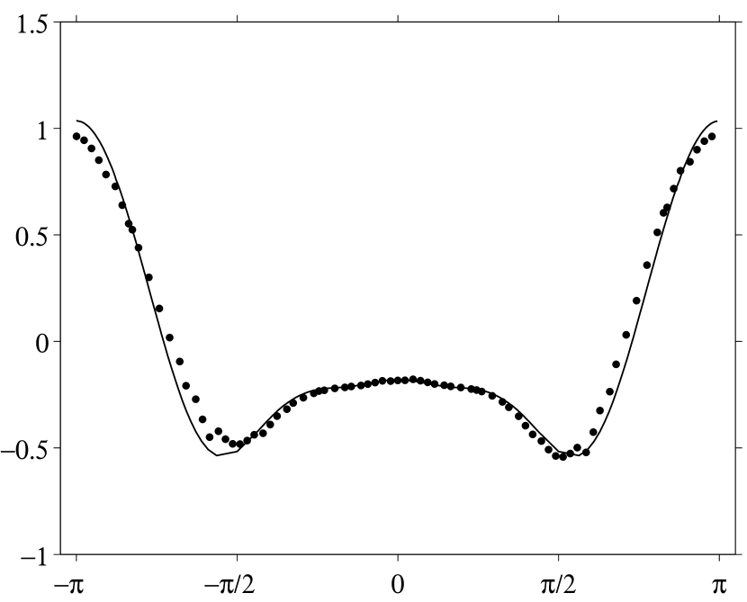
$\theta_{2}$

Figure 26: Data from IBM computations of the steady axisymmetric case ($G=144$). The graphs show profiles of the pressure coefficient $c_{p}$ along two perpendicular great circles on the sphere surface. $(a)$ in a plane given by the vertical direction $\mathbf{e}_{z}$ and $\mathbf{e}_{pH}$; $(b)$ in a plane given by the vertical direction $\mathbf{e}_{z}$ and $\mathbf{e}_{pHz\perp}$. The upstream stagnation point corresponds to a value of the angle $\theta\approx\pm\pi$. Please refer to figure 4 for the location of the great circles and the definition of the angles $\theta_{1}$, $\theta_{2}$. Line styles and symbols indicate: $\bullet$, case BC-24; ——–, reference case BL (taken along dashed lines in figure 9).

Let us now turn to the steady-state results pertaining to the particle motion relative to the ambient fluid, as given in table 7. Here it is again found that the vertical component of the relative velocity, $u_{pV}$, is increasingly well predicted when refining in space. The relative error amounts to 7.7% at $D/\Delta x=15$, to 5.3% at $D/\Delta x=24$ and to 4% at $D/\Delta x=48$. The horizontal component $u_{pH}$, which is non-zero at this Galileo number value, first appears to converge (error decreasing from 4% at $D/\Delta x=15$ to practically zero at $D/\Delta x=24$), but then tends towards a value which is somewhat smaller than the reference result (error of 1.6% at $D/\Delta x=48$). A similar result holds for the angular particle velocity around the horizontal axis perpendicular to the particle motion, $\omega_{pH}$: here the best match is obtained with $D/\Delta x=36$ (error of 0.2%). Finally, it can be seen from table 7 that the error in the prediction of the length of the recirculation region, $L_{r}$, monotonically decreases with spatial resolution (error insignificant at $D/\Delta x=48$). Note that this latter observation is not in contrast to the small discrepancy observed in the projected recirculation length at the highest spatial resolution in figure 23$(b)$, since $L_{r}$ is taken as the maximum extension of the contour with $u_{r\parallel}=0$ downstream of the particle (cf. § 2.4.1).

In order to clarify the non-monotonic behavior of the error with spatial refinement (while keeping the CFL number fixed) observed for $u_{pH}$, $\omega_{pH}$ and for the profile of $u_{r\parallel}$ (taken along the axis parallel to $\mathbf{e}_{p\parallel}$ and passing through the sphere’s center), we have repeated the above simulations with the time step reduced by a factor of 2, i.e. with a maximum CFL number of approximately 0.15. The results for the particle velocities at steady state, obtained with the reduced time step and otherwise identical conditions, are given in table 8 and the axial velocity along the axis downstream of the particle is shown in figure 24. Note that although the particle motion is steady, the results obtained with the present methodology still depend upon the numerical time step $\Delta t$ for two reasons: first, the particle still undergoes a motion with respect to the finite-difference grid, i.e. the flow is non-trivially unsteady in the fixed frame of reference; secondly, the use of a fractional step method introduces a “slip error” on the fluid-solid interface which is of order $\Delta t$ (cf. discussion in Uhlmann, 2005b). From table 8 it can be seen that the respective errors of all particle-related degrees of freedom (except for $u_{pH}$ at $D/\Delta x=48$) behave in a monotonic fashion at this lower value of the CFL number, i.e. decreasing with decreasing grid width $\Delta x$. The observed convergence behavior suggests that there is one contribution to the overall numerical error which is proportional to the ratio $\Delta t/\Delta x$.

The profiles of the three components of the relative velocity $\mathbf{u}_{r}$ in the three local coordinate directions $\mathbf{e}_{p\perp}$, $\mathbf{e}_{pHz\perp}$, $\mathbf{e}_{p\parallel}$ along the lines perpendicular to the axis of particle motion (as indicated by the magenta-colored dashed lines in figure 22$c,d$) are shown in figure 25 for one spatial resolution ($D/\Delta x=24$). The graphs confirm that all aspects of the wake flow are captured with high accuracy by the IBM simulation when a sufficient spatial resolution is applied.

Finally, the surface pressure on the sphere is illustrated in figure 26 by way of the coefficient $c_{p}$ taken along the previously defined two great circles (cf. sketch in figure 4$b,c$). It can be seen that the simulation is able to faithfully capture the shift of the local pressure maximum on the downstream side of the sphere along the great circle which is parallel to $\mathbf{e}_{pHz\perp}$ (i.e. towards small negative values of $\theta_{1}$).

3.2.3 Oscillating oblique regime

$u_{pV}$

$(a)$

$t$

$u_{pH}$

$(b)$

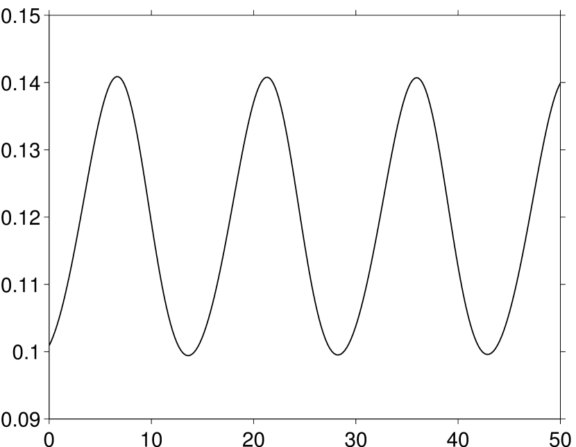
$t$

Figure 27: IBM results for case CC-48 ($G=190.96$, $D/\Delta x=48$), exhibiting time-periodic dynamics. The graphs show the temporal evolution of: $(a)$ the vertical particle velocity component; $(b)$ the horizontal particle velocity component. The corresponding reference data is shown in figure 10.

The extent of the regime in which the particle motion is oblique (with respect to the vertical direction), restricted to a plane in space, and where it is time-periodic spans a relatively narrow range of values of the Galileo number, $185\lesssim G\lesssim 215$ (according to our data from the spectral-element simulations of § 2.4). While defining the relative error at the beginning of § 3.2 we have mentioned the sensitivity of thresholds of bifurcation to numerical accuracy. This is the more true the higher the order of the bifurcation. Since the oscillating oblique regime arises as the result of a secondary bifurcation, a small inaccuracy can induce an upward shift of its threshold by several Galileo number units. Using the present immersed boundary method, simulations using spatial resolutions of $D/\Delta x=24$ and $36$ fail to capture the secondary instability at $G=190$. These simulations yield exponentially decaying oscillations at the correct frequencies showing that the threshold lies above $G=190$. In the following we will present results obtained with a spatial resolution of $D/\Delta x=48$.

The shape of the signals of the translational velocity components ($u_{pV}$ and $u_{pH}$) is shown in figure 27. Comparing the time evolution with the one of the reference signals (cf. figure 10) reveals a very close match. The mean values and fluctuation amplitudes of these periodic signals, as defined in (19-20), as well as the oscillation frequency are shown in table 9. All quantities (including the frequency) are predicted with errors below 4%.

	$D/\Delta x$	$G$	$\overline{u}_{pV}$	$\overline{u}_{pH}$	$\overline{\omega}_{pH}$	$u_{pV}^{\prime}$	$u_{pH}^{\prime}$	$\omega_{pH}^{\prime}$	$f$
CC-48	$48$	$190.96$	$-1.3233$	$0.1201$	$0.0061$	$0.0049$	$0.0207$	$0.0051$	$0.0683$
${\cal E}^{(CC-48)}$			$0.0383$	$0.0116$	$0.0043$	$0.0023$	$0.0089$	$0.0021$	$0.0380$

Table 9: Results from IBM computations of case C (cf. table 1), where $\rho_{p}/\rho_{f}=1.5$ and the nominal value of the Galileo number is $G=190$. The error is computed with respect to the results of the reference case CL (cf. table 4).

$u_{pH}$

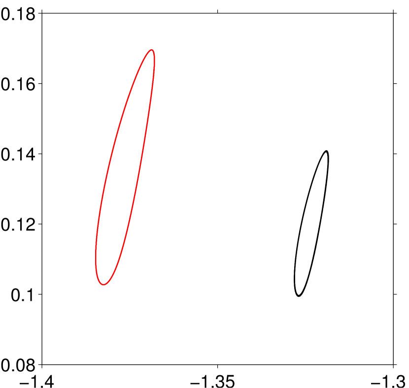
$u_{pV}$

Figure 28: IBM results for case CC ($G=190$), exhibiting time-periodic dynamics. Phase-space plot in the two-dimensional space spanned by the vertical and horizontal particle velocity components. ——–, case CC-48; ——–, reference data (case CL).

Finally, a phase-space plot of horizontal versus vertical particle velocity is shown in figure 28. When equal scaling of the axis is used (as in that figure), the trajectories in phase space have a roughly elliptic shape, with a strong vertical elongation (the fluctuations of the horizontal component are much larger than those of the vertical one), and with a slight inclination with respect to the vertical direction. The IBM results reproduce the shape of the phase-space trajectory very well, albeit at a somewhat smaller scale, i.e. the fluctuation amplitude is generally under-predicted, as obvious from the results shown in table 9. The smaller secondary instability amplitude is to be put, again, on account of the upward shift of the instability threshold.

3.2.4 Chaotic regime

$w_{pr}$

$(a)$

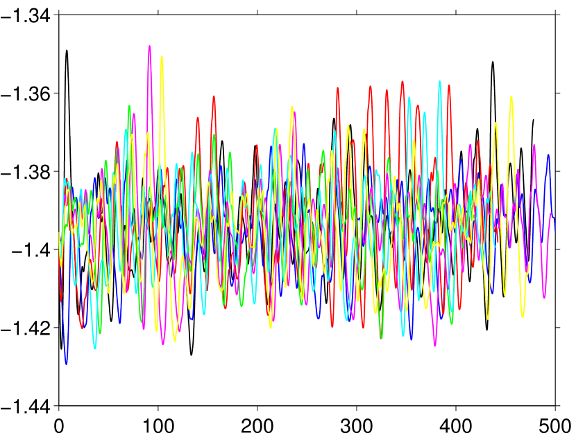
$t$

$u_{pr}$

$(b)$

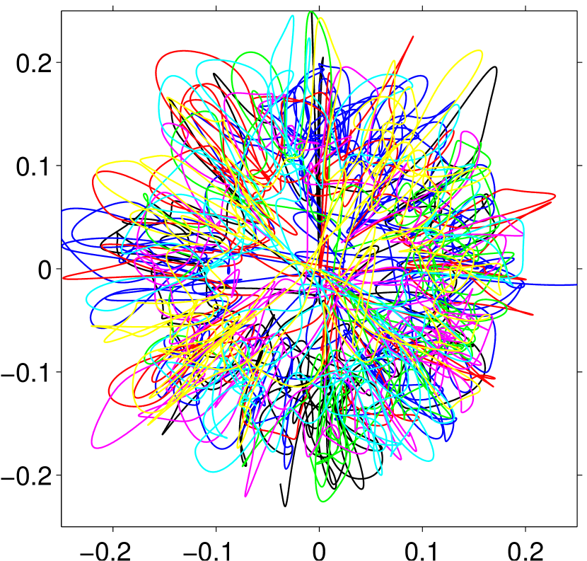
$v_{pr}$

Figure 29: IBM results for case DC-36 ($G=250$), exhibiting chaotic dynamics. $(a)$ Temporal evolution of the vertical particle velocity component (measured relative to the ambient fluid velocity). $(b)$ Phase-space plot in the two-dimensional space spanned by the two horizontal particle velocity components. Each color corresponds to one realization under identical physical and numerical conditions, but starting with different initial fields.

$(a)$

$(b)$

$(c)$

$(d)$

Figure 30: IBM results for case DC-36 ($G=250$), showing an instantaneous flow field. Graphs $(a)$ and $(b)$ show the surface where $u_{r\parallel}=1.2$. Graphs $(c)$ and $(d)$ show the surface where $\lambda_{2}=-0.2$. In $(a)$ and $(c)$ the view is directed along $\mathbf{e}_{pHz\perp}$; in $(b)$ and $(d)$ it is directed along $\mathbf{e}_{pH}$.

In order to capture the chaotic particle motion observed at $G=250$ (cf. § 2.4.5) it was found that a spatial resolution of $D/\Delta x\leq 24$ is not sufficient when employing the present immersed boundary technique. Therefore, we have computed this case with $D/\Delta x=36$.

A number of $N_{runs}=7$ independent realizations has been simulated, each at identical physical and numerical conditions, but starting from a different initial field. The total time simulated amounts to 3570 units. Figure 29$(a)$ shows the time history of the vertical component of the particle velocity relative to the ambient fluid, $w_{pr}$, over the various simulations; figure 29$(b)$ gives an impression of the corresponding trajectories in phase space spanned by the two horizontal components $u_{pr}$ and $v_{pr}$. Both graphs have a similar appearance as the counterparts obtained with the spectral-element method (cf. figure 13). Additionally, the flow field for one snapshot is visualized in figure 30, where iso-surfaces of the relative velocity projected upon the instantaneous particle motion, $u_{r\parallel}$, as well as of $\lambda_{2}$ are shown. Clearly, a similar wake as in the reference case (cf. figure 14) is obtained.

	$D/\Delta x$	$G$	$\langle u_{pV}\rangle$	$\langle u_{pV}^{\prime\prime}u_{pV}^{\prime\prime}\rangle^{1/2}$	$\langle u_{pr}^{\prime\prime}u_{pr}^{\prime\prime}\rangle^{1/2}$	$\langle\omega_{pV}^{\prime\prime}\omega_{pV}^{\prime\prime}\rangle^{1/2}$	$\langle\omega_{px}^{\prime\prime}\omega_{px}^{\prime\prime}\rangle^{1/2}$
DC-36	$36$	$250.00$	$-1.3946$	$0.0129$	$0.0959$	$0.0012$	$0.0136$
${\cal E}^{(DC-36)}$			$0.0451$	$0.0029$	$0.0072$	$0.0000$	$0.0047$

Table 10: Results from IBM computations of case D (cf. table 1), where $\rho_{p}/\rho_{f}=1.5$ and the nominal value of the Galileo number is $G=250$. Note that an ensemble of $N_{runs}=7$ particle paths was analyzed with a total averging interval of $3570$ non-dimensional time units. The error is computed with respect to the results of the reference case DL (cf. table 5).

The mean value of the vertical particle velocity component (relative to the ambient fluid) as well as the rms values of all translational and angular velocity components computed according to the definitions (21-22) are shown in table 10. It is found that the agreement with the reference data is very good. The relative error associated to the mean settling velocity measures 4.5%, while the remaining components are all predicted with errors below one percent. In particular, the rms values are systematically higher in the IBM simulation (except for $\langle\omega_{pV}^{\prime\prime}\omega_{pV}^{\prime\prime}\rangle^{1/2}$). This can be explained by a less chaotic behavior as compared to the reference simulation due to an upward shift of the onset of chaos.

$(a)$

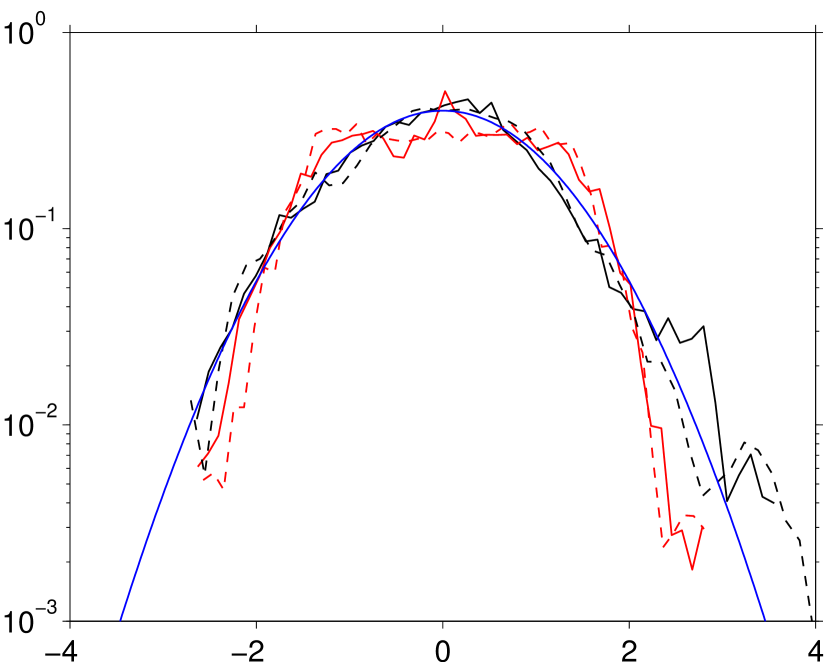
$u_{p\alpha}^{\prime\prime}/\sigma$

$\sigma\cdot pdf$

$\sigma\cdot pdf$

$(b)$

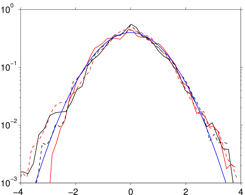
$\omega_{p\alpha}^{\prime\prime}/\sigma$

Figure 31: IBM results for case DC-36 ($G=250$). Probability density functions of: $(a)$ translational particle velocity; $(b)$ angular particle velocity. The line-styles are as follows: ——–, vertical component; ——–, horizontal component; ——–, Gaussian reference curve. The reference data is shown as dashed lines.

The normalized probability density functions corresponding to the translational and angular velocity components are shown in figure 31 alongside the reference data which is included in order to facilitate a direct comparison. It can be seen that – up to the statistical uncertainty inherent in both data-sets – all significant features found in the reference data are reproduced faithfully by the IBM simulation using a spatial resolution of $D/\Delta x=36$. In particular, the plateau-like shape of the pdf of $u_{pH}$ and its sharp drop-off around approximately twice the standard deviation is captured; the same is true for the roughly Gaussian-shaped pdf of $u_{pV}$ and the mild peak around the mean value in $\omega_{pV}$. On the other hand, it can be observed that the horizontal components of the translational and angular particle velocity, $u_{pH}$ and $\omega_{pH}$, exhibit mild peaks around their mean values which are not present in the reference data.

$(a)$

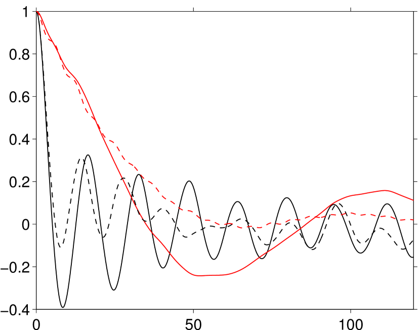
$\tau_{sep}$

$R_{u_{p\alpha}u_{p\alpha}}$

$R_{\omega_{p\alpha}\omega_{p\alpha}}$

$(b)$

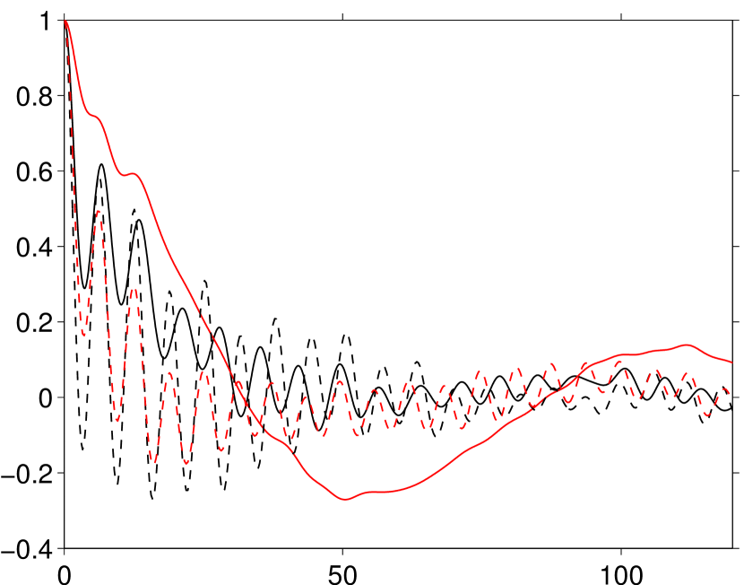
$\tau_{sep}$

Figure 32: IBM results for case DC-36 ($G=250$). Temporal auto-correlations of: $(a)$ translational particle velocity; $(b)$ angular particle velocity. The line-styles are as follows: ——–, vertical component; ——–, horizontal component. The reference data is shown as dashed lines.

Finally, let us turn to the auto-correlations (defined in eqn. 23) of the different particle velocity components shown in figure 32. The auto-correlations of the IBM simulation are characterized by a slower decay as compared to the reference case. This confirms the conjecture that, in the IBM simulation, the threshold of chaos lies closer. Nevertheless, qualitatively the characteristic features of the auto-correlation functions are well reproduced except for that of the horizontal component of the angular velocity. First, the decay rate for short times is very well predicted for both (horizontal and vertical) components. Second, the frequencies of the dominant oscillations are relatively well predicted; in particular, this is true for the fact that the frequency of the oscillation of the vertical component is approximately eight times larger than the one of the horizontal component. It can be observed that the amplitude of the oscillations of the auto-correlation for both translational velocity components is overestimated in the simulations with the immersed boundary method, which is related to a less disordered behavior.

4 Conclusion

We have presented data for the motion of a single solid sphere settling in ambient fluid. The solid to fluid density ratio has been set to $\rho_{p}/\rho_{f}=1.5$, while the Galileo number was varied from 144 to 250 such as to cover all four regimes of sphere motion. The data was generated by means of high-fidelity numerical simulation employing a Fourier/spectral-element method applied to the problem formulated in a coordinate system attached to the sphere, thereby avoiding remeshing (Jenny and Dušek, 2004). A moderately-sized computational domain was chosen in order to keep the computational cost of grid convergence studies tractable.

The data-set provided includes the sphere’s degrees of freedom as well as extracts of the flow field: the recirculation length, the relative velocity along the axis of particle motion and along various cross-profiles, the pressure on the sphere’s surface. In the case of time-periodic motion, the time-evolution of the particle motion as well as that of the flow field in its wake is analyzed in detail. In the case of chaotic particle motion, a statistical analysis of the translational and angular particle velocity is performed, presenting moments, probability density functions and Lagrangian auto-correlation data.

In the second part of this contribution we have presented results of simulations of the above solid-fluid system performed with an immersed boundary method (Uhlmann, 2005a) and using various spatial resolutions varying from 15 points per diameter up to 48. The errors with respect to the reference solution (obtained with the Fourier/spectral-element method) were presented. It was found that a spatial resolution of $D/\Delta x=15$ is capable of reproducing the particle motion in the steady axi-symmetric regime (at $G=144$) with the dominant error measuring approximately 6%. In the steady oblique regime ($G=178.46$) the particular IBM requires a higher resolution of 24 points per diameter in order to produce results of comparable quality. In this case we have also observed that for the immersed boundary method applied in a Navier-Stokes fractional step context the choice of the time step is important in order to achieve the desired accuracy at high spatial resolution. In the regime where the particle motion is still restricted to a plane in space, but varying periodically in time (at $G=190$), a higher spatial accuracy of $D/\Delta x=48$ was necessary in order to capture the state correctly. Finally, it was observed that the chaotic particle motion at $G=250$ can be simulated with good accuracy when using $D/\Delta x=36$. This includes errors committed on the first and second moments of the particle velocity components which are bounded by 4.5%; it also yields a good representation of the probability density functions of particle velocities as well as reasonable auto-correlation functions of translational particle velocity.

The present study provides benchmark data which is expected to be useful for the validation of numerical approaches to finite-size particulate flow. As we have shown, it also provides a basis for determining the required spatial and temporal resolution corresponding to a particular numerical method as a function of the parameter range. As such it can be instrumental in preliminary studies towards simulations of large-scale multi-particle systems where it is often important to determine the minimum numerical requirements for a desired accuracy.

An additional aspect of fluid–particle interaction processes is the presence of turbulent background flow. In that case, direct numerical simulation methods should be able to faithfully take into account the time-dependent multi-scale “forcing” exerted by the turbulent fluid motion upon each particle. Since rigorous benchmark cases for this situation are not available, further efforts should be made in the future to fill this gap.

The data presented herein is available as supplementary material from the journal website. It is also accessible under the following URL:
www.ifh.kit.edu/dns_data/particles/single_sphere_sedimentation

References

- Asmolov (1999) Asmolov, E., 1999. The inertial lift on a spherical particle in a plane Poiseuille flow at large channel Reynolds number. J. Fluid Mech. 381, 63--87.
- Balachandar and Eaton (2010) Balachandar, S., Eaton, J., 2010. Turbulent dispersed multiphase flow. Ann. Rev. Fluid Mech. 42, 111--133.
- Bouchet et al. (2006) Bouchet, G., Mebarek, M., Dušek, J., 2006. Hydrodynamic forces acting on a rigid fixed sphere in early transitional regimes. Eur. J. Mech. B/Fluids 25, 321--336.
- Clift et al. (1978) Clift, R., Grace, J., Weber, M., 1978. Bubbles, drops and particles. Academic Press.
- Ding and Aidun (2000) Ding, E.J., Aidun, C., 2000. The dynamics and scaling law for particles suspended in shear flow with inertia. J. Fluid Mech. 423, 317--344.
- Ern et al. (2012) Ern, P., Risso, F., Fabre, D., Magnaudet, J., 2012. Wake-induced oscillatory paths of bodies freely rising or falling in fluids. Ann. Rev. Fluid Mech. 44, 97--121.
- Fabre et al. (2012) Fabre, D., Tchoufag, J., Magnaudet, J., 2012. The steady oblique path of bouyancy-driven disks and spheres. J. Fluid Mech. 707, 24--36.
- Gao et al. (2013) Gao, H., Li, H., Wang, L.P., 2013. Lattice Boltzmann simulation of turbulent flow laden with finite-size particles. Comp. Math. Appli. 65, 194--210.
- García-Villalba et al. (2012) García-Villalba, M., Kidanemariam, A., Uhlmann, M., 2012. DNS of vertical plane channel flow with finite-size particles: Voronoi analysis, acceleration statistics and particle-conditioned averaging. Int. J. Multiphase Flow 46, 54--74.
- Ghidersa and Dušek (2000) Ghidersa, B., Dušek, J., 2000. Breaking of axisymetry and onset of unsteadiness in the wake of a sphere. J. Fluid Mech. 423, 33--69.
- Horowitz and Williamson (2010) Horowitz, M., Williamson, C.H.K., 2010. The effect of reynolds number on the dynamics and wakes of freely rising and falling spheres. J. Fluid Mech. 651, 251--294.
- Inamuro et al. (2000) Inamuro, T., Maeba, K., Ogino, F., 2000. Flow between parallel walls containing the lines of neutrally buoyant circular cylinders. Int. J. Multiphase Flow 26, 1981--2004.
- Jeffery (1922) Jeffery, G., 1922. The motion of ellipsoidal particles immersed in a viscous fluid. Proc. Roy. Soc. Lond. A 102, 161--179.
- Jenny and Dušek (2004) Jenny, M., Dušek, J., 2004. Efficient numerical method for the direct numerical simulation of the flow past a single light moving spherical body in transitional regimes. J. Comput. Phys. 194, 215--232.
- Jenny et al. (2004) Jenny, M., Dušek, J., Bouchet, G., 2004. Instabilities and transition of a sphere falling or ascending freely in a Newtonian fluid. J. Fluid Mech. 508, 201--239.
- Jeong and Hussain (1995) Jeong, J., Hussain, F., 1995. On the identification of a vortex. J. Fluid Mech. 285, 69--94.
- Johnson and Patel (1999) Johnson, T., Patel, V., 1999. Flow past a sphere up to a Reynolds number of 300. J. Fluid Mech. 378, 19--70.
- Joseph and Ocando (2002) Joseph, D., Ocando, D., 2002. Slip velocity and lift. J. Fluid Mech. 454, 263--286.
- Karniadakis et al. (1991) Karniadakis, G., Israeli, M., Orszag, S., 1991. High-order splitting methods for the incompressible navier-stokes equations. J. Comput. Phys. 97, 414--443.
- Kidanemariam et al. (2013) Kidanemariam, A., Chan-Braun, C., Doychev, T., Uhlmann, M., 2013. DNS of horizontal open channel flow with finite-size, heavy particles at low solid volume fraction. New J. Phys. 15, 025031.
- Kotouč et al. (2008) Kotouč, M., Bouchet, G., Dušek, J., 2008. Loss of axisymmetry in flow past a heated sphere - assisting flow. Int. J. Heat Mass Transfer 51, 2686--2700.
- Lucci et al. (2010) Lucci, F., Ferrante, A., Elghobashi, S., 2010. Modulation of isotropic turbulence by particles of Taylor length-scale size. J. Fluid Mech. 650, 5--55.
- Lucci et al. (2011) Lucci, F., Ferrante, A., Elghobashi, S., 2011. Is Stokes number an appropriate indicator for turbulence modulation by particles of Taylor length-scale size. Phys. Fluids 23, 025101.
- Matas et al. (2004) Matas, J.P., Morris, J., Guazzelli, E., 2004. Inertial migration of rigid spherical particles in Poiseuille flow. J. Fluid Mech. 515, 171--195.
- Mordant and Pinton (2000) Mordant, N., Pinton, J.F., 2000. Velocity measurement of a settling sphere. Eur. Phys. J. B 18, 343--352.
- Mougin and Magnaudet (2002) Mougin, G., Magnaudet, J., 2002. The generalized Kirchhoff equations and their application to the interaction between a rigid body and an arbitrary time-dependent viscous flow. Int. J. Multiphase Flow 28, 1837--1851.
- Pan and Glowinski (2002) Pan, T., Glowinski, R., 2002. Direct simulation of the motion of neutrally buoyant circular cylinders in plane poiseuille flow. J. Comput. Phys. 181, 260--279.
- Patera (1984) Patera, A., 1984. A spectral element method for fluid dynamics: laminar flow in a channel expansion. J. Comput. Phys. 54, 468--488.
- Ten Cate et al. (2004) Ten Cate, A., Derksen, J., Portella, L., Van Den Akker, H., 2004. Fully resolved simulations of colliding monodisperse spheres in forced isotropic turbulence. J. Fluid Mech. 519, 233--271.
- Uhlmann (2005a) Uhlmann, M., 2005a. An immersed boundary method with direct forcing for the simulation of particulate flows. J. Comput. Phys. 209, 448--476.
- Uhlmann (2005b) Uhlmann, M., 2005b. An improved fluid-solid coupling method for DNS of particulate flow on a fixed mesh, in: Sommerfeld, M. (Ed.), Proc. 11th Workshop Two-Phase Flow Predictions, Universität Halle, Merseburg, Germany. ISBN 3-86010-767-4.
- Uhlmann (2006) Uhlmann, M., 2006. Experience with DNS of particulate flow using a variant of the immersed boundary method, in: Wesseling, P., Oñate, E., Périaux, J. (Eds.), Proc. ECCOMAS CFD 2006, TU Delft, Egmond aan Zee, The Netherlands. ISBN 90-9020970-0.
- Uhlmann (2007) Uhlmann, M., 2007. Investigating turbulent particulate channel flow with interface-resolved DNS, in: Sommerfeld, M. (Ed.), ICMF 2007, CDROM, Leipzig, Germany.
- Uhlmann (2008) Uhlmann, M., 2008. Interface-resolved direct numerical simulation of vertical particulate channel flow in the turbulent regime. Phys. Fluids 20, 053305.
- Uhlmann and Doychev (2012) Uhlmann, M., Doychev, T., 2012. Finite size particles in homogeneous turbulence, in: Binder, K., Münster, G., Kremer, M. (Eds.), NIC Symposium 2012, Jülich (Germany). pp. 377--384.
- Veldhuis and Biesheuvel (2007) Veldhuis, C., Biesheuvel, A., 2007. An experimental study of the regimes of motion of spheres falling or ascending freely in a newtonian fluid. Int. J. Multiphase Flow 33, 1074 -- 1087.
- Yang et al. (2005) Yang, B., Wang, J., Joseph, D., Hu, H., Pan, T.W., Glowinski, R., 2005. Migration of a sphere in tube flow. J. Fluid Mech. 540, 109--131.
- Zettner and Yoda (2001) Zettner, C., Yoda, M., 2001. Moderate-aspect-ratio elliptical cylinders in simple shear with inertia. J. Fluid Mech. 442, 241--266.