Can social microblogging be used to forecast intraday exchange rates?

Abstract

The Efficient Market Hypothesis (EMH) is widely accepted to hold true under certain assumptions. One of its implications is that the prediction of stock prices at least in the short run cannot outperform the random walk model. Yet, recently many studies stressing the psychological and social dimension of financial behavior have challenged the validity of the EMH. Towards this aim, over the last few years, internet-based communication platforms and search engines have been used to extract early indicators of social and economic trends. Here, we used Twitter’s social networking platform to model and forecast the EUR/USD exchange rate in a high-frequency intradaily trading scale. Using time series and trading simulations analysis, we provide some evidence that the information provided in social microblogging platforms such as Twitter can in certain cases enhance the forecasting efficiency regarding the very short (intradaily) forex.

1 Introduction

The exchange rate forecasting is one of the most significant, yet tough research pursuits of contemporary financial management. Volatility risk is directly connected not only to company but also to national and international-level macroeconomic relations and strategic measures. Hence, it is not a surprise that markets and organizations such as the Federal Reserve have spent an inordinate amount of both time and money in trying to develop models able to accurately predict the future. Over the years, studies have proceeded mainly on two fronts. On one hand, there are the fundamental models trying to project the exchange rates based on rational expectations hypotheses involving major macroeconomical figures such as national incomes, expected inflation differentials, supplies and demands of the exchanged currencies. This category includes models based on the purchasing power parity (Keneth, 1996), covered and uncovered interest rate parity (Chaboud and Wright, 2005; Chinn et al., 2004) and monetary models (Frankel, 1982; MacDonald and Taylor, 1994; Groen, 2000). However, as Richard Meese and Kenneth Rogoff showed back in 1983 (Meese et al., 1983), such structural models cannot outperform the forecasting capability of a naive random-walk at least in the short run. On the other hand, there are the so-called unstructured models which use time-series statistics to predict currency movements. This category includes regression models (Huang et al., 2005; Preminger and Franck, 2007), Markov models (Mamon and Elliott, 2007; Park, et al., 2009; Shmilovici et al., 2009; Nikolsko-Rzhevskyy and Prodan, 2011), support vector regression (Burges, 1998; Van Gestel et al., 2001; Tay and Cao, 2002; Kim 2003; Huanga et al., 2010), artificial neural networks and genetic algorithms (Kuan and Liu 1995; Yao and Tan, 2000; Liao and Tsao, 2006). Recently, various agent-based models based on behavioral finance concepts (Shleifer, 2000) have been proposed that relax the standard hypothesis of homogeneous perfectly informed agents with expectations consistent with the theoretical ones (Steiglitz and Shapiro, 1998; Carpenter, 2002; Iori, 2002; Marsilia and Raffaelli, 2006; Corona et al., 2008). Indeed, news diffusion and social mimesis through social networking have been, especially over the last few decades, primary factors in shaping not only markets but also economical and political changes around the globe (Garcia, 1997; Hon et al., 2007; Johansen, 2004). Under this perspective, identifying and understanding social collective behavior as this emerges due to individuals’ interactions has become a key element in today’s economy (Camerer, 1999; Daniel et al., 2002; Ross, 2008; Casti, 2010; Knauff et al., 2010). However, also these models, due to the inherent extraordinary complexity of the problem, they are built on incomplete knowledge and for that reason they are flashing a “note of caution” on their robustness and efficiency. As stated by the former Chairman of the Federal Reserve of the United States Alan Greenspan in 2002 “There may be more forecasting of exchange rates, with less success, than almost any other economic variable” (Greenspan, 2002). The efficient market hypothesis (Fama, 1970; Milgrom and Stokey, 1982; Malkiel, 2003, 2005) has been proved by experience to hold true, at least regarding predictions in the short run, in its two common forms: (a) the weak, stating that future prices cannot be predicted by using any technical analysis based on prices from the past and (b) the semi-strong, stating that future prices cannot be predicted based on publicly available new information such as the macroeconomic surprises. But what about the strong form of the EMH reflecting all kinds of information? It has been shown, that if the “beliefs” of the traders are concordant and the agents behave rationally, both private and public information are valueless to speculation (Milgrom and Stokey, 1982). However, there are studies claiming that the celebrated Milgrom and Stokey no-trade theorem does not apply when agents react diversely on public available information. In general, agents exhibit heterogeneity in their behavior, they often respond irrationally and/or diversely in the announcement of public announcements based on their earning expectations and they are diversely informed. Among others, the above facts have raised an intense debate over the validity of the EMH. Regarding forex it has been demonstrated by many studies that “beliefs” as these are shaped by people’s private information play a major role (Bacchetta and van Wincoop, 2006; Gyntelberg et al., 2009). But how one can retrieve such ”private” information? Nolte and Pohlmeier (2006) analyzed the predictive capability of finance experts based on the Centre of European Economic Research’s Financial Markets Survey. They concluded that there is no any evidence that could support the assumption that such a survey could provide valuable information for improving forecasting. Today, the newborn microblogging socializing services - that have revolutionarized the way private and publicly available information diffuses- appear as promising media to data mining agents’ personal information and “beliefs” as these are reflected by their (trading) behavior (Schumaker and Chen, 2009; Asur and Huberman, 2010). For example, such services have been exploited with the aid of search queries as tools to stock-market prediction (Bollen et al., 2011) and movie box-office revenue (Asur and Huberman, 2010); the modeling and prediction of other complex phenomena such as the early detection of epidemics (Ginsberg et al., 2009) and earthquake (Earle et al., 2010) has also been attempted. For financial or macro-economic time series prediction, three general categories of online sources have been exploited (see Mao and Bollen (2011) for a review), namely News Media, Web Search (such as Google Insight) and Social Microblogging (such as Facebook and Twitter). These studies try to form sentiment indicators based on keyword finding and proper interpretation. Here we follow another path in exploiting Twitter’s online data sets: we make use of traders “beliefs” as reflected through their published limit orders in the Twitter. Several on-line algorithmic brokerage firms (e.g. Zulutrade.com) publish the incoming limit orders of their retail clients, (without displaying their identity) for other participants to view, bid and post their own orders. It is therefore tempting to exploit such information to enhance the forecasting potential of exchange rates. Using various kinds of modes, namely Autoregressive (AR), Autoregressive with exogenous input linear models (ARX) and Artificial Neural Networks (ANN) we provide some evidence that social microblogging services can in certain cases be used to enhance the forecasting performance of these models in the very short (intradaily) run.

2 Method’s summary

Our proposed approach aims at providing evidence that social web media such as the Twitter’s microblogging platform can be used to enhance forecasting of the exchange rate in the short run. For our illustrations, we used a dataset of 20,250 public-available messages posted on the Twitter’s platform (with no re-tweets in them) recorded from 25/10/2010 to 05/01/2011. Twitter launched in 2006 providing social networking through the posting of 140-character text messages among its users. Today, the estimated daily traffic is around 65 million tweets sent by more than 190 million users. Each of these tweets was provided along with its identifier (a username), the date and time of the tweet’s submission, and the posted text content. Using a search API on Twitter’s database, the Archivist, we searched the database in order to match the keyword “buy EUR/USD”. Doing so, we found out that each tweet containing the sought string was including information about the types of orders that each Twitter user-trader had made, as well as the target-price of each of these orders. The order types that were posted were in their majority limit orders, that each trader had already made, possibly through his brokerage firm, and thus reflecting his ”belief” about the upcoming EUR/USD exchange rate quote. Using the target-price of each message, we first transformed each obtained number into an integer, in order to form a solid dataset. This has been done, because many target-prices were posted in different forms, i.e. as “1.345” or “1,345”, “13,45”, “134.5” etc. Due to the fact that our analysis was focused on high-frequency intraday trading, we decided to study the temporal behavior of the tweets in an hourly basis. As many recent financial studies have proposed, regarding the distribution of several financial assets (J.P. Morgan Asset Management, 2009), we found that the intradaily tweets’ -based quotes distribution follows also an alpha-stable distribution. At this point we should note that within our sample, there were a few days (3 out of 54 trading days) lacking a statistically significant number of observations (due to the fact that Twitter Archivist didn’t seem to collect many tweets during these days). To overcome the problem and just for these days, we produced a larger sample, filling the trading hours within these days, using the alpha-stable distribution with the same statistical parameters of the other days (such as variance, skewness etc.), except for the statistical mean value. This was taken to be the Gaussian weighted-with respect to the transaction volume- mean of the few tweets recorded in each of these days. In order to predict the actual closing based on the tweets trend, we used a time window of the first 50 minutes within each hour. For example, for the tweets posted from 1 to 2.00 pm, we selected the tweets posted from 1.01 pm until 1.51 pm. Figure 1 depicts the time series of the tweets’ quotes and those of the hourly actual closing exchange EUR/USD rates as obtained from the Yahoo Finance database.

Figure 1: Time series of the tweets’ quotes (grey region) and those of the hourly actual closing exchange EUR/USD rates (solid line) as obtained from the Yahoo Finance database.

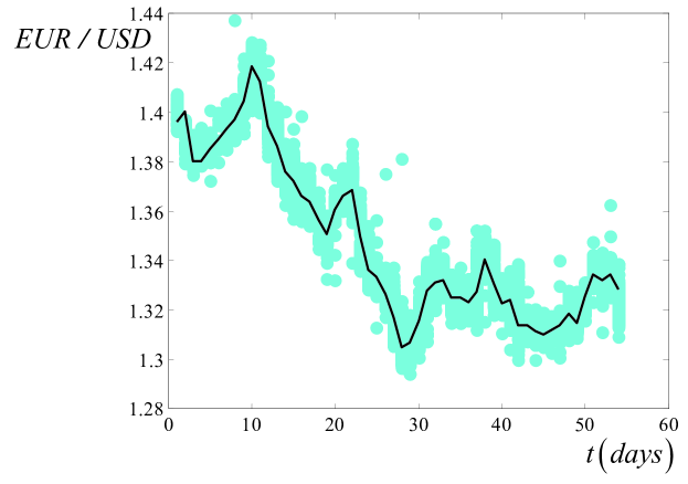
By applying statistical tests (Anderson -Darling and Kolmogorov), we found that both distributions for the total period of the 54 trading days are hyperbolic-like distributions. More specifically, the tweet’s distribution gave a best fit to a hyperbolic distribution with statistical mean, 1.3475 and sigma, 0.021, while for the actual closing distribution these values were mean, 1.3488 and sigma, 0.023.

3 The Models

We explored the forecasting potential of the information contained in the tweets, and compared their prediction efficiency by constructing (a) autoregressive (AR) (b) autoregressive exogenous (ARX) linear models and (c) multilayered feedforward neural networks (ANN).
The general form of the AR models reads:

$$\hat{A}(z^{-1})y(t)=e(t)$$ (1)

Here, $y(t)$ denotes the actual EUR/USD exchange rate at time $t$ (hourly basis); $e(t)$ is the residual at time $t$ representing the part of the measurement that cannot be predicted from previous measurements.

$$\hat{A}(z^{-1})=a_{0}+a_{1}z^{-1}+a_{2}z^{-2}+...+a_{n_{a}}z^{-n_{a}}$$ (2)

$z^{-1}$ is the backward shift operator defined by

$$z^{-k}y(t)=y(t-k)\\$$ (3)

The ARX models can be written as:

$$y(t)=A(z^{-1})y(t-n_{k})+B(z^{-1})u(t-n_{k})+e(t)$$ (4)

Here, $u(t)$ denotes the mean value of the quotes based on the tweets as computed within the 50 minutes time interval before the time $t$; $n_{k}$ is the pure time delay and

$$\begin{split}A(z^{-1})=a_{1}+a_{2}z^{-1}+a_{3}z^{-2}+...+a_{n_{a}}z^{-n_{a}}\\ B(z^{-1})=b_{1}+b_{2}z^{-1}+b_{3}z^{-2}+...+b_{n_{b}}z^{-n_{b}}\end{split}$$ (5)

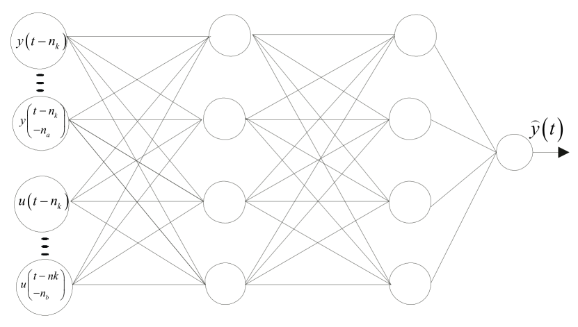
For comparison purposes, we also used nonlinear regressors, namely two-layer feedforward neural networks (ANNs). The ANNs were constructed with two hidden layers with four nodes for each layer and threshold functions given by $f(x)=2/(1+e^{-2x})-1$. Hence, there are $n_{a}+n_{b}$ neurons in the input layer, and one neuron in the output layer with a pure linear function (see Figure 2 for a schematic of the ANN).

Figure 2: Schematic of the ANN model

The network was trained for 100 epochs with the back-propagation algorithm based on the mean square of errors (Rumelhart et al., 1986). Using different numbers of neurons (e.g. 3,5,6) for each hidden layer did not change the outcomes of the analysis. For any practical means, given the size of a training set, say, $N_{T}$, in order to achieve a fair interpolation of the input space and to avoid undesirable phenomena such as overfitting, the total number of weights in the network, say $N_{w}$ should satisfy the condition $N_{w}<eN$, where $e$ is the expected average approximating error (Baum and Haussler, 1988).

The data set containing the actual closing rates and the coarse-grained values of the tweets was split in two sets: one containing the first $60\%$ of the data serving as a training set, $N_{T}$ and the other one containing the last $40\%$ of the data serving as a test set, say $N_{V}$. Different choices of the sizes of the training and validation data sets did not change the outcomes of the analysis.
The parameter estimation of both types of models was done by least-squares fitting on the set of both raw data (at level) and exchange/ tweets rate returns defined by $y^{\prime}=100\log{y(t)}-\log{y(t-1)}$ and $u^{\prime}=100\log{u(t)}-\log{u(t-1)}$ , respectively. Data differentiation accounts the problem of non-stationarity and trends, thus eliminating potential biases in forecasting.

We evaluated the forecasting performance of the above models on both kind of test sets (at level and differentiated), through (a)fixed-forecasting-horizon metrics, and, (b) trading simulations. In particular, we used three fixed-forecasting-horizon metrics:
(i)the root mean square error metric defined by

$$RMSE=\sqrt{\frac{1}{N_{V}}(\sum_{t=1}^{N_{V}}e(t)^{2})}$$ (6)

(ii) the mean absolute error defined by

$$MAE=\frac{1}{N_{V}}\sum_{t=1}^{N_{V}}|e(t)|$$ (7)

where $e(t)=\hat{y}(t)-y(t)$, $\hat{y}(t)$ is the prediction and $y(t)$ is the actual closing rate at time $t$; other metrics such as the mean square error were also used leading to the same conclusions.
(iii) directional change statistics, namely

(a) for the analysis of the actual at level data, the average number of ups and downs which are correctly forecasted, defined by

$$DA=\frac{1}{N_{V}}\sum_{i=1}^{N_{V}}a(t)$$ (8)

where

$$a(t)=\left\{\begin{array}[]{cc}1,\ if\ (y(t)-y(t-n_{k}))(\hat{y}(t)-y(t-n_{k}))>0\\ 0,\ otherwise\end{array}\right\}\\$$ (9)

(b) for the analysis of the return rates (log-differentiated data), the average number of signs that are correctly forecasted defined by

$$Sgn=\frac{1}{N_{V}}\sum_{i=1}^{N_{V}}b(t)$$ (10)

where

$$b(t)=\left\{\begin{array}[]{cc}1,\ if\ (\hat{y^{\prime}}(t)y^{\prime}(t))>0\\ 0,\ otherwise\end{array}\right\}\\$$ (11)

Our trading simulations involved the computation of the return profits defined by,

$$R(t)=\sigma(t)\frac{y(t)-y(t-n_{k})}{y(t-n_{k})}100\\$$ (12)

Here we used the simple mving average trading rule reading:

$$\sigma(t)=\left\{\begin{array}[]{cc}1,\ if\ \hat{y}(t)>\overline{y(t)}_{m}\\ -1,\ if\ \hat{y}(t)<\overline{y(t)}_{m}\end{array}\right\}\\$$ (13)

where

$\overline{y(t)}_{m}$ is the m-order moving average defined as

$$\overline{y(t)}_{m}=\frac{1}{m}\sum_{i=0}^{m-1}y(t-i)\\$$ (14)

4 Time Series Analysis and Trading Simulations: Results and Discussion

Regarding the at level time series, the values of the parameters of the AR models and their standard deviations as obtained for different values of $n_{a}$ and $n_{k}=1$ are given in table 1.

Table 1: At level data series: Coefficients of the AR models fitted with the training dataset

	$a_{1}$	$a_{2}$	$a_{3}$	$a_{4}$	$a_{5}$	$a_{6}$	$a_{7}$	$a_{8}$	$a_{9}$	$a_{10}$
$n_{a}=1$	-1
$n_{a}=2$	-1.0047	0.0048
$n_{a}=3$	-1.0014	-0.0875	0.08914
$n_{a}=4$	-1	-0.0802	0.1044	-0.024
$n_{a}=5$	-1	-0.0761	0.1013	-0.0646	0.0397
$n_{a}=6$	-0.9976	-0.078	0.1068	-0.0687	-0.022	0.0598
$n_{a}=7$	-1.0014	-0.0768	0.11010	-0.0753	-0.0172	0.1209	-0.0601
$n_{a}=8$	-0.9934	-0.0923	0.1119	-0.0648	-0.0339	0.1321	0.0719	-0.1312
$n_{a}=9$	-0.9997	-0.0895	0.1199	-0.0669	-0.0314	0.1341	0.0693	-0.1852	0.0496
$n_{a}=10$	-0.995	-0.0997	0.1221	-0.0597	-0.0335	0.13512	0.0723	-0.1875	0.00297	0.0429

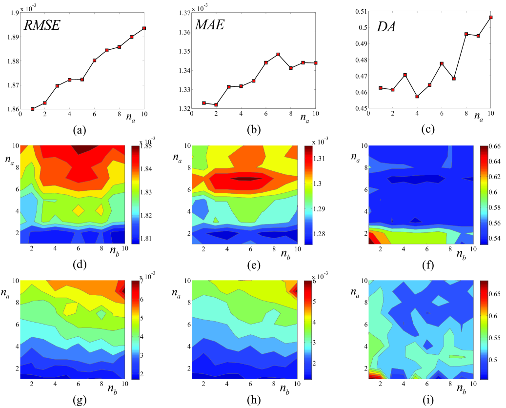
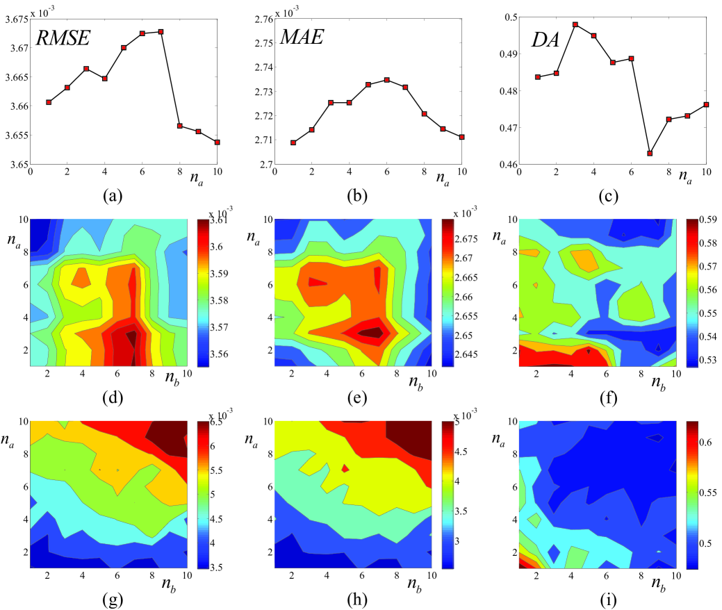
Figures 3a,b,c summarize the resulting $RMSEs$, $MAEs$, $DAs$ for the AR models with respect to $n_{a}$ and $n_{k}=1$.
Based on the $RMSE$, $MAE$, we found that for one-step time forecasting horizons the random walk model defined by $a_{1}=-1,a_{2}=...a_{n_{a}}=0$ cannot be outperformed by any other AR model (Figure 3a,b). The $RMSE$ for the random walk model was 0.00186, the $MAE$ was 0.0013; the variance of the prediction error distribution was $\approx 3.45E^{-6}$. Any other AR model with $n_{a}>1$ gave greater or almost equal $RMSEs$, $MAEs$ than the ones obtained with the random walk model. Incorporating now the information from the Twitter’s database in the ARX models (defined by $n_{a}>0$,$n_{b}>0$) we constructed the 2-dimensional contour plots of the computed $RMSE$, $MAE$ and $DA$ (Figures 3d,e,f) for $n_{k}=1$ and $n_{a}$,$n_{b}$ ranging from 1 to 10. It is shown that the best ARX predictors were in the range of $n_{a}=1,2$ and $n_{b}=2-10$ giving $RMSEs$ around 0.00181, $MAE$ around 0.00128, $DA$ around 0.65; the variances of the estimation errors were around $3.8E^{-6}$. The simulations results indicate that no ARX model could significantly outperform the random walk model in terms of the $RMSE$ and $MAE$. In fact, the apparent best ARX predictor with $n_{a}=2$,$n_{b}=10$ gave a $RMSE$ equal to 0.00181 which is slightly better than the one obtained with the naive random walk. However, the one-way analysis of variance statistical test for the mean of the distribution of estimation errors between the random walk and the best ARX predictor showed no significant difference. In terms of the $DA$ metric though, it is shown that the ARX models with $n_{a}=1,2$,$n_{b}=1-8$ resulted to significant higher values compared to the one of the random walk (see Figure 3f). In particular, for this range of parameters the $DA$ ranged from 0.67 (for $n_{a}=1$,$n_{b}=1$) to 0.6 (for $n_{a}=1$,$n_{b}=7$). The values of the ARX coefficients as well as their uncertainty (standard deviation) for $n_{a}=1$ and $n_{b}=7$ are given in Table 2.

Table 2: At level data: Coefficients and their standard deviation of the ARX model with $n_{a}=1,n_{b}=7$

$a_{0}=0.97357(\pm 0.0099)$	$b_{0}=0.0334(\pm 0.0132)$	$b_{1}=-0.0265(\pm 0.0153)$
$b_{2}=0.01634(\pm 0.0152)$	$b_{3}=-0.00388(\pm 0.01498)$	$b_{4}=-0.00309(\pm 0.01495)$
$b_{5}=0.00622(\pm 0.0149)$	$b_{5}=-0.0172(\pm 0.0149)$	$b_{6}=0.02099(\pm 0.0128)$

Similar results with the above were obtained using the ANN models. Figures 3g,h,i summarize the corresponding $RMSEs$, $MAEs$ and $DAs$. The best ANN predictors were found for $n_{a}=1$ and $n_{b}=1,2$ with $RMSE$ around 0.0017, $MAE$ around 0.00123 and $DA$ around 0.65. For this range of parameters the variances of the estimation errors were around $3E^{-6}$).
The above results indicate that the information contained in the Twitter could be used to enhance the forecasting efficiency in the short (intradaily) run.

Figure 3: At level data analysis: $RMSEs$((a),(d),(g)), $MAEs$((b),(e),(h)) and $DAs$ ((c),(f),(i)) for the AR, ARX and ANN models respectively with respect to the orders $n_{a}$ and $n_{b}$ with $n_{k}=1$

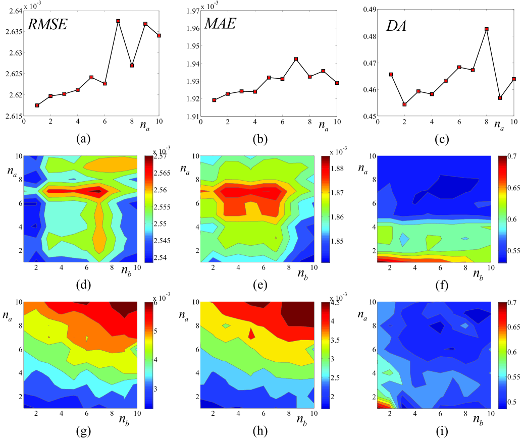
We also performed computations with other forecasting horizons defined by $n_{k}>1$. For illustration purposes, Figures 4,5 summarize the $RMSEs$, $MAEs$ and $DAs$ for $n_{k}=2$ and $n_{k}=4$, respectively as computed with AR, ARX and ANN models. The corresponding variances are around $1E^{-5}$ for both ARX and ANNs models. As it is shown the ARX and ANN models outerperform the naive random walk with respect of all metrics when $n_{k}>1$. However, this should be attributed to the apparent trend in the actual/raw at level data. It is interesting though to remark, that even at relatively long forecasting time horizons (e.g. for $n_{k}=4$) the information contained in the twitters enhances significantly the forecasting performance(see e.g. Figures 5f,g,h).

Figure 4: At level data analysis: $RMSEs$((a),(d),(g)), $MAEs$((b),(e),(h)) and $DAs$ ((c),(f),(i)) for the AR, ARX and ANN models respectively with respect to the order $n_{a}$ and $n_{b}$ with $n_{k}=2$

Figure 5: At level data analysis: $RMSEs$((a),(d),(g)), $MAEs$((b),(e),(h)) and $DAs$ ((c),(f),(i)) for the AR, ARX and ANN models respectively with respect to the orders $n_{a}$ and $n_{b}$ with $n_{k}=4$

We also performed trading simulations in which the “traders” use the estimated price as obtained by the forecast of the models and produce a “buy” signal ($s=1$) if the estimation is above the current moving average actual closing, and a “sell” signal $(s=-1)$ otherwise as described in the previous section. Figure 6a shows the cumulative return of the random walk model for $m=4$, $nk=1$. As it is shown the trading simulations result to cumulative loses.

Figure 6: Cumulative returns derived with the moving average trading simulation (with moving average horizon defined by $m=4$) for a one step forecasting horizon ($n_{k}=1$) using (a) the random walk model, (b) a ANN model with $n_{a}=3$ and $n_{b}=6$

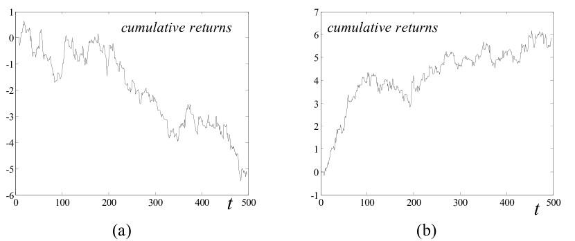
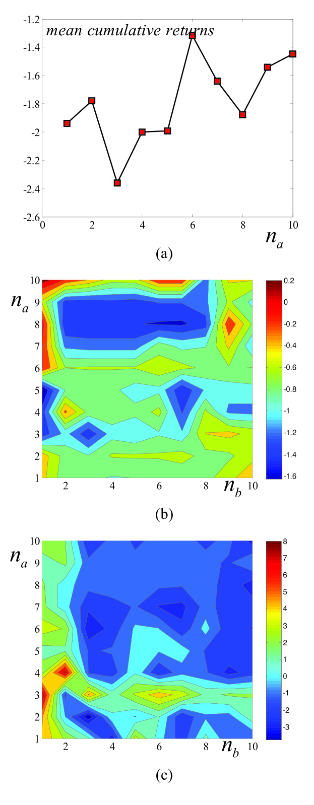
Figure 7a illustrates the mean values of the computed cumulative returns for $m=4$, $nk=1$ when using the AR models. Figures 7b,c show the contour plots of the mean values of the cumulative returns computed with the trading simulations for $m=4$, $nk=1$ with the ARX and ANN models, respectively. The trading simulations, indicate that the tweets incorporated in the ARX and ANN models carry information that enhances the forecasting ability resulting, for certain values of the orders $n_{b}$ and $n_{a}$, into profitable trading opportunity, thus outerperforming the AR models (which lack information from tweets). Indicatevely, in Figure 6b we illustrate the cumulative returns obtained by the moving average trading simulation for one-step forecasting horizon ($n_{k}=1$) using a ANN model with $n_{a}=3$ and $n_{b}=6$.

Figure 7: Mean Cumulative returns derived with the moving average Trading simulation ($m=4$ and $n_{k}=1$) using the (a) AR, (b) ARX, (c) ANN models

At this point we should note that the above results are due to trending in the at level data. To test if the forecasting efficiency of the ARX and ANN models employing information contained in the twitter’s database perform better than the naive random walk and generally the AR models when trend is excluded, we also performed the same analysis using the detrended data as derived by log-differencing. Figures 8,9,10 depict the computed $RMSEs$,$MAEs$ and $Sgns$ for the AR, ARX and ANN models for the exchange/ tweets rate returns (log-differences), for $n_{k}=1$, $n_{k}=2$ and $n_{k}=4$, respectively (the orders $n_{a}$,$n_{b}$ ranged from 1 to 10). For $n_{k}=1$ the random walk gives the minimum $RMSE$ and $MAE$ (around 0.1405 for $RMSE$ and 0.1 for $MAE$) compared to the other AR models. For the same time lag, the best ARX model ($n_{a}=1$,$n_{b}=8-10$)gave around 0.1372 for $RMSE$ and 0.0975 for $MAE$. The corresponding $RMSE$ and $MAE$ values of the best ANN model ($n_{a}=1$,$n_{b}=2$ were 0.1361 for $RMSE$ and 0.098 for $MAE$. One-way Anova test between the mean values of the estimation errors from the best ARX and ANN models and the random walk showed no significant difference. The same behaviour is observed for other $n_{k}>1$. For example, for $n_{k}=4$ the random walk gives the minimum $RMSE$ and $MAE$ (around 0.140 for $RMSE$ and 0.1 for $MAE$) compared to the other AR models. For the same time lag, the best ARX model ($n_{a}=1$,$n_{b}=6$)gave around 0.1395 for $RMSE$ and 0.1 for $MAE$. The corresponding values of the best ANN model ($n_{a}=6$,$n_{b}=6$ were 0.1361 for $RMSE$ and 0.0986 for $MAE$. Again one-way Anova test between the mean values of the estimation errors from the best ARX and ANN models and the random walk showed no significant difference.In terms of directional change statistics s described by the $Sgn$ describing the proportion of times that the model forecasts correctly the sign of change in the rates, the AR models for $n_{k}=1$ result to values of $Sgn$ around 0.5 (the random walk gives around 0.53). However, it is interesting to note that some ARX and ANN models incorporating the information contained in the tweets produced considerably higher values of $Sgn$ up to 0.59 for (see Figure 8f,i).

Figure 8: Rate returns (log-differences)analysis: $RMSEs$((a),(d),(g)), $MAEs$((b),(e),(h)) and $Sgns$ ((c),(f),(i)) for the AR, ARX and ANN models respectively with respect to the orders $n_{a}$ and $n_{b}$ with $n_{k}=1$

Figure 9: Rate returns (log-differences) analysis: $RMSEs$((a),(d),(g)), $MAEs$((b),(e),(h)) and $Sgns$ ((c),(f),(i)) for the AR, ARX and ANN models respectively with respect to the orders $n_{a}$ and $n_{b}$ with $n_{k}=2$

Figure 10: Rate returns (log-differences) analysis: $RMSEs$((a),(d),(g)), $MAEs$((b),(e),(h)) and $Sgns$ ((c),(f),(i))for the AR, ARX and ANN models respectively with respect to the orders $n_{a}$ and $n_{b}$ with $n_{k}=4$

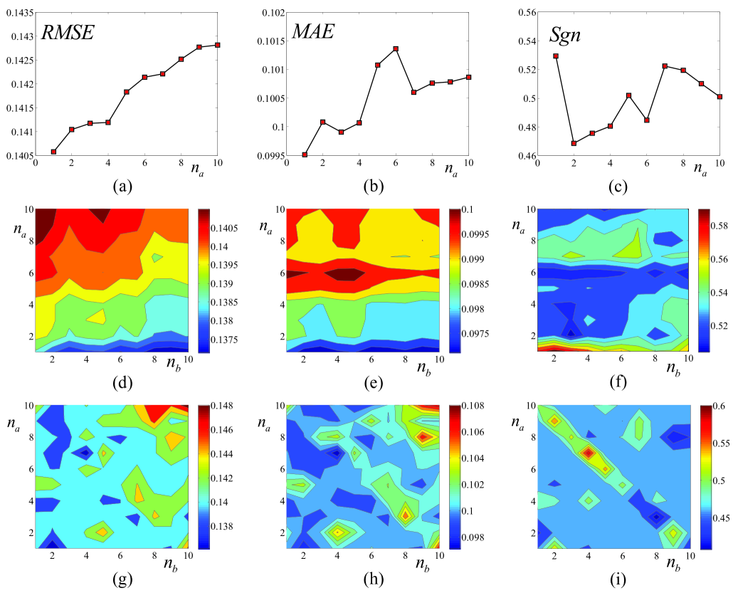
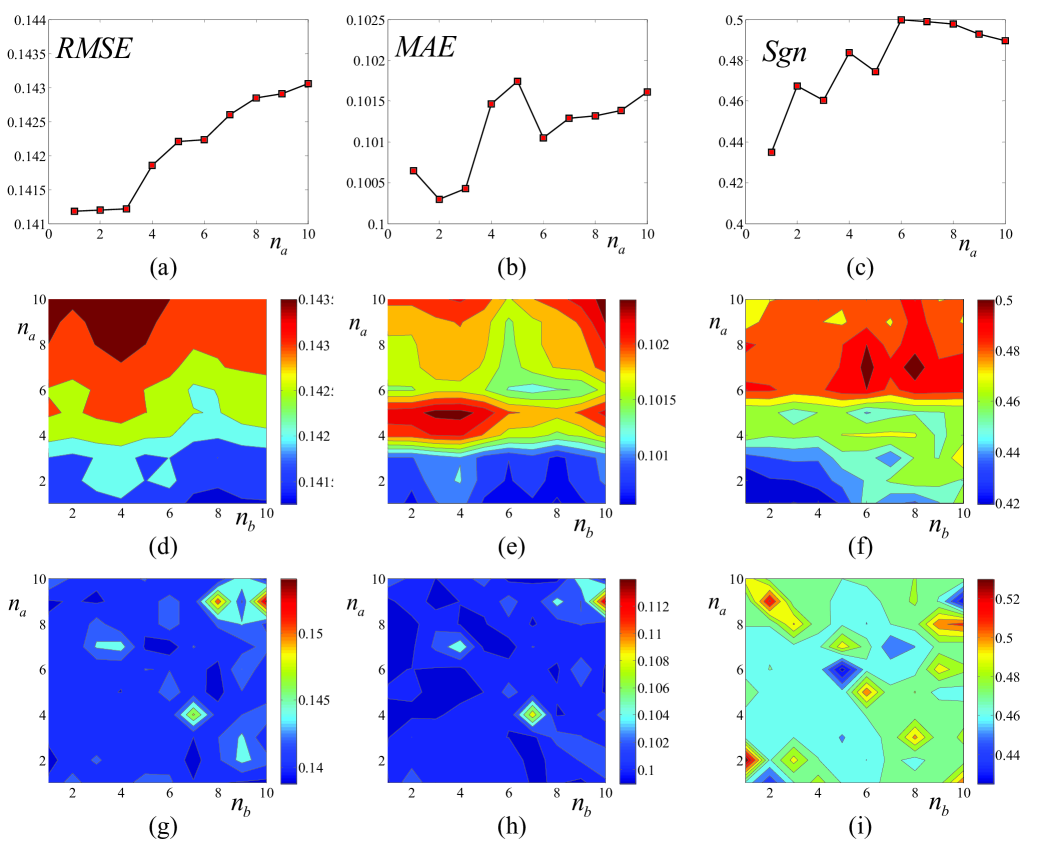
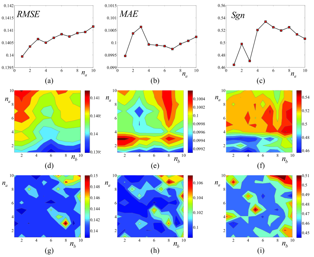
In particular, the best ARX models, with respect to the $Sgn$ statistic, was found for $n_{a}=1$, $n_{b}=1-4$, $n_{k}=1$ giving values of $Sgn$ from 0.574 ($n_{a}=1$, $n_{b}=4$) up to 0.596 ($n_{a}=1$, $n_{b}=2$) (Figure 8f). The best ANN performance is observed for $n_{a}=7$, $n_{b}=4$ and $n_{k}=1$ giving a value of $Sgn$ around 0.6 (see Figure 8i). In order to test the statistical significance of the results produced by the best ARX and ANN models we performed bootstrapping on a total of 5000 randomly perturbed resamples of the validation data. Simulations were performed for $n_{k}=1$ using the best ARX model (with $n_{a}=1$, $n_{b}=2$) and the best ANN model (with $n_{a}=7$, $n_{b}=4$). The resulting empirical bootstrap distributions of the $Sgns$ obtained by the ARX and ANN models on the 5000 resamples are illustrated in Figure 11a,b, respectively.

Figure 11: Empirical Bootstrapping distributions of $Sgns$ for $n_{k}=1$ using (a) the ARX(with $n_{a}=1$, $n_{b}=2$), (b) the ANN (with $n_{a}=7$, $n_{b}=4$ produced from 5000 bootstrapped resamples of the validation data

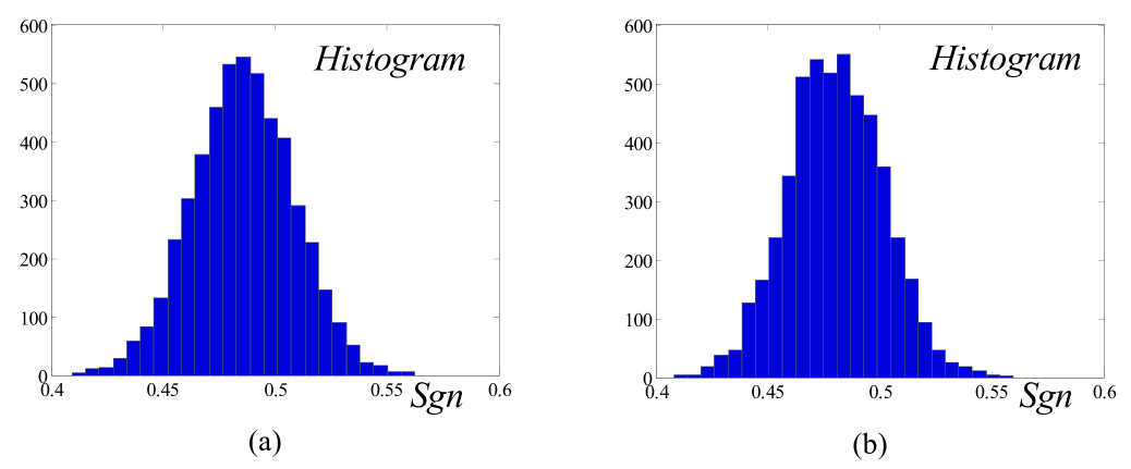
As it is clearly seen the values obtained with the best ARX and ANN models are well beyond the maximum values of the resulting bootstrap distributions. These results indicate that the information of the tweets can be used to enhance the forecasting efficiency of the directional change of the rates. For large values of the forecasting horizon i.e. for $n_{k}>1$ no significant differences were observed (the values of $Sgns$ were around 0.5 with small deviations) (see Figures 8c,f,i and Figures 9c,f,i)

5 Conclusions

Over the last years it has been demonstrated that social media such as web-based search engines and recently Twitter can be used to forecast certain future complex events. In a similar fashion, an unresolved problem in contemporary monetary and economical management research, the foreign currency exchange rate forecasting (forex) in the short run, might be also benefit from the use of social microblogging. In this work we attempted to test the validity of the Efficient Market Hypothesis in its strong form with respect to forex through Twitters’ social networking communication platform. We explored the possibility of using private (yet, publicly available through a microblogging platform) information of market players that could be used to outerperform the EMH in the very short term dictating that the market is inefficient, as far as the overall information flow to investors is concerned. In particular, we attempted to give an answer to the following basic question: can information behavior contained in the context of microblogging and the “belief” of traders be used to enhance the forecasting efficient and outperform the random walk? To our knowledge this is the first time that such an analysis is provided for the forecast of the exchange rate of EUR/USD. We believe that our study is of significant importance, as the contemporary research in the area trying to contradict the EMH is focused on the uncovering of market anomalies as these may arise by the information flow provided by the market players’ “beliefs” in the social networks. Towards this direction, the development of several psychological indexes that are related to market’s consensus, is already in great use by players as well as market’s regulators. Our analysis showed that the rate exchange forecasting at level, based on people’s beliefs as these can be data-mined through microblogging may carry significant information that can used to outperform the random walk hypothesis and AR models that do not include such information but solely past values of the exchange rates, in the very short run. This was also demonstrated through moving average trading simulations. However, we should note that this behaviour should be attributed to the underlying trend of the data. This is apparent when encountering larger forecasting horizons. When the analysis was performed on the return rates (log-differencing), i.e. a log-differencing of the actual values which accounts the problem of non-stationarity and trends, the analysis showed significant difference with respect to forecasting efficiency of directional changes as described by the proportion of times that the relative directional changes of signs are correctly forecasted for one-step-time forecasting horizon. Regarding any conclusions that can be extracted by our analysis, we should refer to its certain assumptions and restrictions. For example we used (a) a data-base deploying within a limited period of time that did not include any major anomaly, (b) our forecasting was targeted solely in the very short (intradaily) horizon, (c) no risk assessment analysis was taken into account, (d) we used just black-box time series models, (e) we used only a small part of the social microblogging platforms reported data. In addition, evaluating forecasting efficiency and accuracy remain an important issue for further research. For example, out-of-sample statistical measures can be improved using rolling-origin evaluations and re-calibration of optimal coefficients based on new data sets (see Tashman (2000) for a review and critical discussion). Concluding, we believe that social networks can provide the basis for further advances in the field and thus enable the formalization of the experimental side of the market’s psychology as this is shaped by the human behavior. Towards this aim detailed Agent-based models analysed by state-of-the-art multiscale techniques (see e.g. Tsoumanis et al. (2010), Siettos et al.(2012))have the potential to facilitate computational modeling and exploration - and thus our understanding and forecasting market’s complex dynamics.

References

- (1) Almenberg, J., Kittlitz, K. and Pfeiffer, T., An experiment on prediction markets in science, PLoS ONE, 4, e8500 (2009).
- (2) Asur, S. and Huberman, B.A., Predicting the future with social media, arXiv:1003.5699v1 (2010).
- (3) Bacchetta, P. and van Wincoop, E., Can information heterogeneity explain the exchange rate determination puzzle?, American Economic Review, 96, 552-576 (2003).
- (4) Baum, E. B. and Haussler, D., What size gives valid generalization, Neural Computation, 1, 151-160 (1988).
- (5) Bollen, J., Mao, H. and Zeng, X. J., Twitter mood predicts the stock market, J. of Computational Science, 2, 1-8 (2011).
- (6) Burges, J. C., A Tutorial on support vector machines for pattern recognition, Data Mining and Knowledge Discovery, 2, 121-167 (1998).
- (7) Camerer, C., Behavioral economics: Reunifying psychology and economics, Proc. Natl. Acad. Sci. USA, 96, 10575-10577 (1999).
- (8) Carpenter, J. P., Evolutionary models of bargaining: Comparing agent-based computational and analytical approaches to understanding convention evolution, Computational Economics, 19, 25-49 (2002).
- (9) Casti, J., Mood Matters, Springer NY (2010).
- (10) Chaboud, A. P. and Wright, J. H., Uncovered interest parity: it works, but not for long, Journal of International Economics, 66, 349-362 (2005).
- (11) Chinn, M. D. and Meredith, G., Monetary policy and long horizon uncovered interest parity, IMF Staff Papers, 51, 409-430 (2004).
- (12) Corona, E., Ecca, S., Marchesi, M. and Setzu, A., The interplay between two stock markets and a related foreign exchange market: a simulation approach, Computational Economics, 32, 99-119 (2008).
- (13) Daniel, K., Hirshleifer, D. and Teoh, S. H., Investor psychology in capital markets: evidence and policy implications, Journal of Monetary Economics, 49, 139-209 (2002).
- (14) Earle, P., Guy, M., Buckmaster, R., Ostrum, C., Horvath, S. and Vaughan, A., OMG Earthquake! Can Twitter improve earthquake response?, Seismological Research Letters, 81, 246-251 (2010).
- (15) Fama, E. F., Efficient capital markets: a review of theory and empirical work, Journal of Finance, 25, 383-417 (1970).
- (16) Frankel, J. A., The mystery of the multiplying marks: a modification of the 36 monetary model, The Review of Economics and Statistics, 64, 515-519 (1982).
- (17) Garcia, V. F., Black December, banking instability, the Mexican crisis and its effect on Argentina, World Bank Publications, Washington, DC (1997).
- (18) Ginsberg, J., Mohebbi, M. H., Patel, R. S., Brammer, L., Smolinski, M. S. and Brilliant, L., Black December, banking instability, the Mexican crisis and its effect on Argentina, Detecting influenza epidemics using search engine query data, Nature, 457,1012-1014 (2009).
- (19) Greenspan, A. , Testimony of the Federal Reserve Board’s semiannual monetary policy report to the Congress, before the Committee on Banking, Housing, and Urban Affairs, Monetary policy report, U.S. Senate (2002).
- (20) Groen, J. J., The Monetary exchange rate model as a long-run phenomenon, Journal of International Economics, 52, 299-319 (2000).
- (21) Gyntelberg, J., Loretan, M., Subhanij, T. and Chan, E., Private information, stock markets, and exchange rates, BIS Working Papers from Bank for International Settlements, No 271 (2009).
- (22) Hon, M. T., Strauss, J. K. and Yong, S. K., Deconstructing the Nasdaq bubble: A look at contagion across international stock markets, Journal of International Financial Markets, Institutions and Money, 17, 213-230 (2007).
- (23) Huang, C.M., Huang, C. J. and Wang, M. L., A particle swarm optimization to identifying the ARMAX model for short-term load forecasting, IEEE Transactions on Power Systems, 20, 1126 1133 (2005).
- (24) Huanga, S., Chuanga, C., Wub, C. F. and Laia, H. J., Chaos-based support vector regressions for exchange rate forecasting, Expert Systems with Applications, 37, 8590-8598 (2010).
- (25) Iori, G., A microsimulation of traders activity in the stock market: the role of heterogeneity, agents interactions and trade frictions, Journal of Economic Behavior & Organization, 49, 269 285 (2002).
- (26) Johansen, A., Origin of crashes in three US stock markets: shocks and bubbles, Physica A, 338, 135-142 (2004).
- (27) Keneth, R., The Purchasing power parity puzzle, Journal of Economic Literature, 24, 647-668 (1996).
- (28) Kim, K., Financial time series forecasting using support vector machines, Neurocomputing, 55, 307 319 (2003).
- (29) Knauff, M., Budeck, C., Wolf, A. G. and Hamburger, K., The illogicality of stock-brokers: psychological experiments on the effects of prior knowledge and belief biases on logical reasoning in stock trading, PLoS ONE, 5, e13483 (2010).
- (30) Kuan, C. M. and Liu, T., Forecasting exchange rates using feedforward and recurrent neural networks, Journal of Applied Econometrics, 10, 347-364 (1995).
- (31) Liao, G. C. and Tsao, T. P., Application of a fuzzy neural network combined with a chaos genetic algorithm and simulated annealing to short term load forecasting, IEEE Transactions on Evolutionary Computation, 10, 330 340 (2006).
- (32) Linrong, D., Market behaviors and dynamic evolution on heterogeneous agent clusters, Physica A, 376, 573 578 (2007).
- (33) MacDonald, R. and Taylor, M. P., The monetary model of the exchange rate: Long-run relationships, short-run dynamics and how to beat a random walk, Journal of International Money and Finance, 13, 276 290 (1994).
- (34) Malkiel, B. G., Reflections on the efficient market hypothesis: 30 Years Later, The Financial Review, 40, 1 9 (2005).
- (35) Malkiel, B. G., The Efficient ffmarket hypothesis and its critics, The Journal of Economic Perspectives, 17, 59 82 (2003).
- (36) Mamon, R. S. and Elliott, R. J., Hidden Markov models in finance, International Series in Operations Research & Management Science, Springer, NY (2007).
- (37) Mao, H.and Bollen, J.,Predicting financial markets: comparing survey, news,Twitter and Search Engine Data, arxiv:1112.1051v1 (2011).
- (38) Marsilia, M. and Raffaelli, G., Risk bubbles and market instability, Physica A, 370, 18 22 (2006).
- (39) Meese, R. A. and Rogoff, K., Empirical exchange rate models of the seventies: Do they fit out-of-sample?, Journal of International Economics, 14, 3-24 (1983).
- (40) Milgrom, P. and Stokey, N., Information, trade and common knowledge, Journal of Economic Theory, 26, 17-27 (1982).
- (41) Nikolsko-Rzhevskyy, A. and Prodan, R., Markov switching and exchange rate predictability, International Journal of Forecasting, doi:10.1016/j.ijforecast.2011.04.007 (2011).
- (42) Nolte, I. and Pohlmeier, W., Using forecasts of forecasters to forecast, International Journal of Forecasting, 23, 15-28 (2006).
- (43) Park, S. H., Lee, J. H., Song, J. W. and Park, T. S., Forecasting change directions for financial time series using hidden Markov model, Lecture Notes in Computer Science, 5589, 184-191 (2009).
- (44) Preminger, A. and Franck, R., Forecasting exchange rates: a robust regression approach, International Journal of Forecasting, 23, 71-84 (2007).
- (45) Ross, D., Cognitive science and social cognition, Cognitive Systems Research, 9, 125-135 (2008).
- (46) Rumelhart, E. E., Hinton, G. E. and Williams, R. J., Learning representations by back-propagating errors, Nature 323, 533 536 (1986).
- (47) Schumaker, R. P. and Chen H., Textual analysis of stock market prediction using breaking financial news: The AZFin text system, ACM Transactions on Information Systems, 27, 1 12 (2009).
- (48) Shleifer, A., Inefficient Markets: An introduction to behavioral finance, Oxford University Press, UK (2000).
- (49) Shmilovici, A., Kahiri, Y., Ben-Gal, I. and Hauser, S., Measuring the efficiency of the intraday forex market with a universal data compression algorithm, Computational Economics, 33, 131-154 (2009).
- (50) Steiglitz, K. and Shapiro, D., Simulating the madness of crowds: price bubbles in an auction-mediated robot market, Computational Economics, 12, 35-59 (1998).
- (51) Tay, E. H. F. and Cao, L. J., Modified support vector machines in financial time series forecasting, Neurocomputing, 48, 847-861 (2002).
- (52) Tashman, L. J., Out-of-sample tests of forecasting accuracy: An analysis and review, International Journal of Forecasting, 16, 437-450 (2000).
- (53) Tsoumanis, A.C., Siettos, C.I., Kevrekidis, I.G., Bafas, G.V., Equation-Free Multiscale Computations in Social Networks: from Agent-based Modelling to Coarse-grained Stability and Bifurcation Analysis, Int. J. Bifurcation and Chaos, 20, 3673-3688 (2010).
- (54) Siettos, C. I., Gear, C. W., Kevrekidis, I. G., An Equation-free Approach to Agent-Based Computation: Bifurcation Analysis and Control of Stationary States, EPL (Europhysics Letters), 99, 48007 (2012).
- (55) Van Gestel, T., Suykens, K. J., Baestaens, D., Lambrechts, A., Lanckriet, G., Vandaele, B., De Moor, B. and Vandewalle, J., Financial time series prediction using least squares support vector machines within the evidence framework, IEEE Transactions on Neural Networks, 12, 809-821 (2001).
- (56) Yao, J. T. and Tan, C. L., A case study on using neural networks to perform technical forecasting of forex, Neurocomputing, 34, 79-98 (2000).