Abstract

Gaussian processes are typically used for smoothing and interpolation on small datasets. We introduce a new Bayesian nonparametric framework – GPatt – enabling automatic pattern extrapolation with Gaussian processes on large multidimensional datasets. GPatt unifies and extends highly expressive kernels and fast exact inference techniques. Without human intervention – no hand crafting of kernel features, and no sophisticated initialisation procedures – we show that GPatt can solve large scale pattern extrapolation, inpainting, and kernel discovery problems, including a problem with $383400$ training points. We find that GPatt significantly outperforms popular alternative scalable Gaussian process methods in speed and accuracy. Moreover, we discover profound differences between each of these methods, suggesting expressive kernels, nonparametric representations, and exact inference are useful for modelling large scale multidimensional patterns.

 

GPatt: Fast Multidimensional Pattern Extrapolation with Gaussian Processes

 

1 Introduction

“The future of the human enterprise may well depend on Big Data”, exclaimed West (2013), writing for Scientific American. Indeed we have quickly entered an era of big data, focussing recent machine learning efforts on developing scalable models for large datasets, with notable results from deep neural architectures (Krizhevsky et al., 2012).

Neural networks first became popular in the 1980s because they allowed for adaptive basis functions, as opposed to the fixed basis functions in well known linear models. With adaptive basis functions, neural networks could automatically discover interesting structure in data, while retaining scalable learning procedures (Rumelhart et al., 1986). But this newfound expressive power came at the cost of interpretability and the lack of a principled framework for deciding upon network architecture, activation functions, learning rates, etc., all of which greatly affect performance.

Following neural networks came the kernel era of the 1990s, where infinitely many fixed basis functions were used with finite computational resources via the kernel trick – implicitly representing inner products of basis functions using a kernel. Kernel methods are flexible, and often more interpretable and manageable than neural network models. For example, Gaussian processes can be used as rich prior distributions over functions with properties – smoothness, periodicity, etc. – controlled by an interpretable covariance kernel. Indeed Gaussian processes have had success on challenging non-linear regression and classification problems (Rasmussen, 1996).

Within the machine learning community, Gaussian process research developed out of neural networks research. Neal (1996) argued that since we can typically improve the performance of a model by accounting for additional structure in data, we ought to pursue the limits of large models. Accordingly, Neal (1996) showed that Bayesian neural networks become Bayesian nonparametric Gaussian processes with a neural network kernel, as the number of hidden units approach infinity. Thus Gaussian processes as nonparametric kernel machines are part of a natural progression, with the flexibility to fit any dataset, automatically calibrated complexity (Rasmussen & Williams, 2006; Rasmussen & Ghahramani, 2001), easy and interpretable model specification with covariance kernels, and a principled probabilistic framework for learning kernel hyperparameters.

However, kernel machines like Gaussian processes are typically unable to scale to large modern datasets. Methods to improve scalability usually involve simplifying assumptions, such as finite basis function expansions (Lázaro-Gredilla et al., 2010; Williams & Seeger, 2001; Le et al., 2013; Rahimi & Recht, 2007), or sparse approximations using pseudo (inducing) inputs (Snelson & Ghahramani, 2006; Hensman et al., 2013; Seeger et al., 2003; Quiñonero-Candela & Rasmussen, 2005). While these methods are promising, they simplify standard Gaussian process models, which are sometimes already too simple, particularly when a large number of training instances are available to learn sophisticated structure in data.

Indeed popular covariance kernels used with Gaussian processes are not often expressive enough to capture rich structure in data and perform extrapolation, prompting MacKay (1998) to ask whether we had “thrown out the baby with the bathwater”. In general, choice of kernel profoundly affects the performance of a Gaussian process – as much as choice of architecture affects the performance of a neural network. Typically, Gaussian processes are used either as flexible statistical tools, where a human manually discovers structure in data and then hard codes that structure into a kernel, or with the popular Gaussian (squared exponential) or Matérn kernels. In either case, Gaussian processes are used as smoothing interpolators, only able to discover limited covariance structure. Likewise, multiple kernel learning (Gönen & Alpaydın, 2011) typically involves hand crafting combinations of Gaussian kernels for specialized applications, such as modelling low dimensional structure in high dimensional data, and is not intended for automatic pattern discovery and extrapolation.

In this paper we propose a scalable and expressive Gaussian process framework, GPatt, for automatic pattern discovery and extrapolation on large multidimensional datasets. We begin, in Section 2, with a brief introduction to Gaussian processes. In Section 3 we then introduce expressive interpretable kernels, which build off the recent kernels in Wilson & Adams (2013), but are especially structured for multidimensional inputs and for the fast exact inference and learning techniques we later introduce in Section 4. These inference techniques work by exploiting the existing structure in the kernels of Section 3 – and will also work with popular alternative kernels. These techniques relate to the recent inference methods of Saatchi (2011), but relax the full grid assumption made by these methods. This exact inference and learning costs $\mathcal{O}(PN^{\frac{P+1}{P}})$ computations and $\mathcal{O}(PN^{\frac{2}{P}})$ storage, for $N$ datapoints and $P$ input dimensions, compared to the standard $\mathcal{O}(N^{3})$ computations and $\mathcal{O}(N^{2})$ storage associated with a Cholesky decomposition.

In our experiments of Section 5 we combine these fast inference techniques and expressive kernels to form GPatt. Our experiments emphasize that, although Gaussian processes are typically only used for smoothing and interpolation on small datasets, Gaussian process models can in fact be developed to automatically solve a variety of practically important large scale pattern extrapolation problems. GPatt is able to discover the underlying structure of an image, and extrapolate that structure across large distances, without human intervention – no hand crafting of kernel features, no sophisticated initialisation, and no exposure to similar images. We use GPatt to reconstruct large missing regions in pattern images, to restore a stained image, to reconstruct a natural scene by removing obstructions, and to discover a sophisticated 3D ground truth kernel from movie data. GPatt leverages a large number of training instances ($N>10^{5}$) in many of these examples.

We find that GPatt significantly outperforms popular alternative Gaussian process methods on speed and accuracy stress tests. Furthermore, we discover profound behavioural differences between each of these methods, suggesting that expressive kernels, nonparametric representations, and exact inference – when used together – are useful for large scale multidimensional pattern extrapolation.

2 Gaussian Processes

A Gaussian process (GP) is a collection of random variables, any finite number of which have a joint Gaussian distribution. Using a Gaussian process, we can define a distribution over functions $f(x)$,

$$f(x)\sim\mathcal{GP}(m(x),k(x,x^{\prime}))\,.$$ (1)

The mean function $m(x)$ and covariance kernel $k(x,x^{\prime})$ are defined as

$$m(x) =\mathbb{E}[f(x)]\,,$$ (2)

$$k(x,x^{\prime}) =\text{cov}(f(x),f(x^{\prime}))\,,$$ (3)

where $x$ and $x^{\prime}$ are any pair of inputs in $\mathbb{R}^{P}$. Any collection of function values has a joint Gaussian distribution,

$$[f(x_{1}),\dots,f(x_{N})]\sim\mathcal{N}({\boldsymbol{\mathbf{\mu}}},K)\,,$$ (4)

with mean vector ${\boldsymbol{\mathbf{\mu}}}_{i}=m(x_{i})$ and $N\times N$ covariance matrix $K_{ij}=k(x_{i},x_{j})$.

Assuming Gaussian noise, e.g. observations $y(x)=f(x)+\epsilon(x)$, $\epsilon(x)=\mathcal{N}(0,\sigma^{2})$, the predictive distribution for $f(x_{*})$ at a test input $x_{*}$, conditioned on ${\boldsymbol{\mathbf{y}}}=(y(x_{1}),\dots,y(x_{N}))^{\top}$ at training inputs $X=(x_{1},\dots,x_{n})^{\top}$, is analytic and given by:

$$f(x_{*})|x_{*},X,{\boldsymbol{\mathbf{y}}} \sim\mathcal{N}(\bar{f}_{*},\text{V}[f_{*}])$$ (5)

$$\bar{f}_{*} ={\boldsymbol{\mathbf{k}}}_{*}^{\top}(K+\sigma^{2}I)^{-1}{\boldsymbol{\mathbf{y}}}$$ (6)

$$\text{V}[f_{*}] =k(x_{*},x_{*})-{\boldsymbol{\mathbf{k}}}_{*}^{\top}(K+\sigma_{n}^{2}I)^{-1}{\boldsymbol{\mathbf{k}}}_{*}\,,$$ (7)

where the $N\times 1$ vector ${\boldsymbol{\mathbf{k}}}_{*}$ has entries $({\boldsymbol{\mathbf{k}}}_{*})_{i}=k(x_{*},x_{i})$.

The Gaussian process $f(x)$ can also be analytically marginalised to obtain the likelihood of the data, conditioned only on the hyperparameters ${\boldsymbol{\mathbf{\theta}}}$ of the kernel:

$$\log p({\boldsymbol{\mathbf{y}}}|{\boldsymbol{\mathbf{\theta}}})\propto-[\overbrace{{\boldsymbol{\mathbf{y}}}^{\top}(K_{{\boldsymbol{\mathbf{\theta}}}}+\sigma^{2}I)^{-1}{\boldsymbol{\mathbf{y}}}}^{\text{model fit}}+\overbrace{\log|K_{{\boldsymbol{\mathbf{\theta}}}}+\sigma^{2}I|}^{\text{complexity penalty}}]\,.$$ (8)

This marginal likelihood in Eq. (8) pleasingly compartmentalises into automatically calibrated model fit and complexity terms (Rasmussen & Ghahramani, 2001), and can be optimized to learn the kernel hyperparameters ${\boldsymbol{\mathbf{\theta}}}$, or used to integrate out ${\boldsymbol{\mathbf{\theta}}}$ using MCMC (Murray & Adams, 2010). The problem of model selection and learning in Gaussian processes is “exactly the problem of finding suitable properties for the covariance function. Note that this gives us a model of the data, and characteristics (such as smoothness, length-scale, etc.) which we can interpret.” (Rasmussen & Williams, 2006).

The popular squared exponential (SE) kernel has the form

$$k_{\text{SE}}(x,x^{\prime})=\text{exp}(-0.5||x-x^{\prime}||^{2}/\ell^{2})\,.$$ (9)

GPs with SE kernels are smoothing devices, only able to learn how quickly sample functions vary with inputs $x$, through the length-scale parameter $\ell$.

3 Kernels for Pattern Discovery

The heart of a Gaussian process model is its kernel, which encodes all inductive biases – what sorts of functions are likely under the model. Popular kernels are not often expressive enough for automatic pattern discovery and extrapolation. To learn rich structure in data, we now present highly expressive kernels which combine with the scalable exact inference procedures we will introduce in Section 4.

In general it is difficult to learn covariance structure from a single Gaussian process realisation, with no assumptions. Most popular kernels – including the Gaussian (SE), Matérn, $\gamma$-exponential, and rational quadratic kernels (Rasmussen & Williams, 2006) – assume stationarity, meaning that they are invariant to translations in the input space $x$. In other words, any stationary kernel $k$ is a function of $\tau=x-x^{\prime}$, for any pair of inputs $x$ and $x^{\prime}$.

Bochner’s theorem (Bochner, 1959) shows that any stationary kernel $k(\tau)$ and its spectral density $S(s)$ are Fourier duals:

$$k(\tau) =\int S(s)e^{2\pi is^{\top}\tau}ds\,,$$ (10)

$$S(s) =\int k(\tau)e^{-2\pi is^{\top}\tau}d\tau\,.$$ (11)

Therefore if we can approximate $S(s)$ to arbitrary accuracy, then we can also approximate any stationary kernel to arbitrary accuracy, and we may have more intuition about spectral densities than stationary kernels. For example, the Fourier transform of the popular SE kernel in Eq. (9) is a Gaussian centred at the origin. Likewise, the Fourier transform of a Matérn kernel is a $t$ distribution centred at the origin. These results provide the intuition that arbitrary additive compositions of popular kernels have limited expressive power – equivalent to density estimation with, e.g., scale mixtures of Gaussians centred on the origin, which is not generally a model one would use for density estimation. Scale-location mixtures of Gaussians, however, can approximate any distribution to arbitrary precision with enough components (Kostantinos, 2000), and even with a small number of components are highly flexible models.

Suppose that the spectral density $S(s)$ is a scale-location mixture of Gaussians,

$$S(s)=\sum_{a=1}^{A}w_{a}^{2}[\mathcal{N}(s;\mu_{a},\sigma_{a}^{2})+\mathcal{N}(-s;\mu_{a},\sigma_{a}^{2})]/2\,,$$ (12)

noting that spectral densities for real data must be symmetric about $s=0$ (Hörmander, 1990), and assuming that $x$, and therefore also $s$, are in $\mathbb{R}^{1}$. If we take the inverse Fourier transform (Eq. (11)) of this spectral density in Equation (12), then we analytically obtain the corresponding spectral mixture (SM) kernel function:

$$k_{\text{SM}}(\tau) =\sum_{a=1}^{A}\!w_{a}^{2}\!\exp\{-2\pi^{2}\tau^{2}\sigma_{a}^{2}\}\cos(2\pi\tau\mu_{a})\,,$$ (13)

which was derived by Wilson & Adams (2013), and applied solely to simple time series examples with a small number of datapoints. We extend this formulation for tractability with large datasets and multidimensional inputs.

Many popular stationary kernels for multidimensional inputs decompose as a product across input dimensions. This decomposition helps with computational tractability – limiting the number of hyperparameters in the model – and like stationarity, provides a restriction bias that can help with learning. For higher dimensional inputs, $x\in\mathbb{R}^{P}$, we propose to leverage this useful product assumption, inherent in many popular kernels, for a spectral mixture product (SMP) kernel

$$k_{\text{SMP}}(\tau|{\boldsymbol{\mathbf{\theta}}})=\prod_{p=1}^{P}k_{\text{SM}}(\tau_{p}|{\boldsymbol{\mathbf{\theta}}}_{p})\,,$$ (14)

where $\tau_{p}$ is the $p^{\text{th}}$ component of $\tau=x-x^{\prime}\in\mathbb{R}^{P}$, ${\boldsymbol{\mathbf{\theta}}}_{p}$ are the hyperparameters $\{\mu_{a},\sigma_{a}^{2},w_{a}^{2}\}_{a=1}^{A}$ of the $p^{\text{th}}$ spectral mixture kernel in the product of Eq. (14), and ${\boldsymbol{\mathbf{\theta}}}=\{{\boldsymbol{\mathbf{\theta}}}_{p}\}_{p=1}^{P}$ are the hyperparameters of the SMP kernel. With enough components $A$, the SMP kernel of Eq. (14) can model any product kernel to arbitrary precision, and is flexible even with a small number of components. We use SMP-A as shorthand for an SMP kernel with $A$ components in each dimension (for a total of $3PA$ kernel hyperparameters and $1$ noise hyperparameter).

4 Fast Exact Inference

In this Section we present algorithms which exploit the existing structure in the SMP kernels of Section 3, and many other popular kernels, for significant savings in computation and memory, but with the same exact inference achieved with a Cholesky decomposition.

Gaussian process inference and learning requires evaluating $(K+\sigma^{2}I)^{-1}{\boldsymbol{\mathbf{y}}}$ and $\log|K+\sigma^{2}I|$, for an $N\times N$ covariance matrix $K$, a vector of $N$ datapoints ${\boldsymbol{\mathbf{y}}}$, and noise variance $\sigma^{2}$, as in Equations (6) and (8), respectively. For this purpose, it is standard practice to take the Cholesky decomposition of $(K+\sigma^{2}I)$ which requires $\mathcal{O}(N^{3})$ computations and $\mathcal{O}(N^{2})$ storage, for a dataset of size $N$. However, nearly any kernel imposes significant structure on $K$ that is ignored by taking the Cholesky decomposition.

For example, many kernels separate multiplicatively across $P$ input dimensions:

$$k(x_{i},x_{j})=\prod_{p=1}^{P}k^{p}(x_{i}^{p},x_{j}^{p})\,.$$ (15)

We show how to exploit this structure to perform exact inference and hyperparameter learning in $\mathcal{O}(PN^{\frac{2}{P}})$ storage and $\mathcal{O}(PN^{\frac{P+1}{P}})$ operations, compared to the standard $\mathcal{O}(N^{2})$ storage and $\mathcal{O}(N^{3})$ operations. We first assume the inputs $x\in\mathcal{X}$ are on a multidimensional grid (Section 4.1), meaning $\mathcal{X}=\mathcal{X}_{1}\times\dots\times\mathcal{X}_{P}\subset\mathbb{R}^{P}$, and then relax this grid assumption in Section 4.2.

4.1 Inputs on a Grid

Many real world applications are engineered for grid structure, including spatial statistics, sensor arrays, image analysis, and time sampling.

Assuming a multiplicative kernel and inputs on a grid, we find

1. $K$ is a Kronecker product of $P$ matrices (a Kronecker matrix) which can undergo eigendecomposition into $QVQ^{\top}$ with only $\mathcal{O}(PN^{\frac{2}{P}})$ storage and $\mathcal{O}(PN^{\frac{3}{P}})$ computations (Saatchi, 2011).

2. The product of Kronecker matrices such as $K$, $Q$, or their inverses, with a vector ${\boldsymbol{\mathbf{u}}}$, can be performed in $\mathcal{O}(PN^{\frac{P+1}{P}})$ operations.

Given the eigendecomposition of $K$ as $QVQ^{\top}$, we can re-write $(K+\sigma^{2}I)^{-1}{\boldsymbol{\mathbf{y}}}$ and $\log|K+\sigma^{2}I|$ in Eqs. (6) and (8) as

$$(K+\sigma^{2}I)^{-1}{\boldsymbol{\mathbf{y}}} =(QVQ^{\top}+\sigma^{2}I)^{-1}{\boldsymbol{\mathbf{y}}}$$ (16)

$$=Q(V+\sigma^{2}I)^{-1}Q^{\top}{\boldsymbol{\mathbf{y}}}\,,$$ (17)

and

$$\log|K+\sigma^{2}I|=\log|QVQ^{\top}+\sigma^{2}I|=\sum_{i=1}^{N}\log(\lambda_{i}+\sigma^{2})\,,$$ (18)

where $\lambda_{i}$ are the eigenvalues of $K$, which can be computed in $\mathcal{O}(PN^{\frac{3}{P}})$.

Thus we can evaluate the predictive distribution and marginal likelihood in Eqs. (5) and (8) to perform exact inference and hyperparameter learning, with $\mathcal{O}(PN^{\frac{2}{P}})$ storage and $\mathcal{O}(PN^{\frac{P+1}{P}})$ operations (assuming $P>1$).

4.2 Missing Observations

Assuming we have a dataset of $M$ observations which are not necessarily on a grid, we can form a complete grid using $W$ imaginary observations, ${\boldsymbol{\mathbf{y}}}_{W}\sim\mathcal{N}({\boldsymbol{\mathbf{f}}}_{W},\epsilon^{-1}I_{W})$, $\epsilon\to 0$. The total observation vector ${\boldsymbol{\mathbf{y}}}=[{\boldsymbol{\mathbf{y}}}_{M},{\boldsymbol{\mathbf{y}}}_{W}]^{\top}$ has $N=M+W$ entries: ${\boldsymbol{\mathbf{y}}}=\mathcal{N}({\boldsymbol{\mathbf{f}}},{D_{N}})$, where

$${D}_{N}=\left[\begin{array}[]{cc}{D}_{M}&0\\ 0&{\epsilon}^{-1}{I}_{W}\end{array}\right],$$ (21)

and $D_{M}=\sigma^{2}I_{M}$. The imaginary observations ${\boldsymbol{\mathbf{y}}}_{W}$ have no corrupting effect on inference: the moments of the resulting predictive distribution are exactly the same as for the standard predictive distribution in Eq. (5). E.g., $(K_{N}+D_{N})^{-1}{\boldsymbol{\mathbf{y}}}=(K_{M}+D_{M})^{-1}{\boldsymbol{\mathbf{y}}}_{M}$.

We use preconditioned conjugate gradients (PCG) (Atkinson, 2008) to compute $\left(K_{N}+{D}_{N}\right)^{-1}{\boldsymbol{\mathbf{y}}}$. We use the preconditioning matrix ${C}={D}_{N}^{-1/2}$ to solve ${C}^{\top}\left(K_{N}+{D}_{N}\right){C}{\boldsymbol{\mathbf{z}}}={C}^{\top}{\boldsymbol{\mathbf{y}}}$. The preconditioning matrix $C$ speeds up convergence by ignoring the imaginary observations ${\boldsymbol{\mathbf{y}}}_{W}$. Exploiting the fast multiplication of Kronecker matrices, PCG takes $\mathcal{O}(JPN^{\frac{P+1}{P}})$ total operations (where the number of iterations $J\ll N$) to compute $\left(K_{N}+{D}_{N}\right)^{-1}{\boldsymbol{\mathbf{y}}}$, which allows for exact inference.

For learning (hyperparameter training) we must evaluate the marginal likelihood of Eq. (8). We cannot efficiently decompose $K_{M}+D_{M}$ to compute the $\log|K_{M}+D_{M}|$ complexity penalty in the marginal likelihood, because $K_{M}$ is not a Kronecker matrix, since we have an incomplete grid. We approximate the complexity penalty as

$$\log|K_{M}+D_{M}| =\sum_{i=1}^{M}\log({\lambda}_{i}^{M}+\sigma^{2})$$ (22)

$$\approx\sum_{i=1}^{M}\log(\tilde{\lambda}_{i}^{M}+\sigma^{2})\,.$$ (23)

We approximate the eigenvalues $\lambda_{i}^{M}$ of $K_{M}$ using the eigenvalues of $K_{N}$ such that $\tilde{\lambda}_{i}^{M}=\frac{M}{N}\lambda_{i}^{N}$ for $i=1,\dots,M$, which is a particularly good approximation for large $M$ (e.g. $M>1000$) (Williams & Seeger, 2001). We emphasize that only the log determinant (complexity penalty) term in the marginal likelihood undergoes a small approximation, and inference remains exact.

All remaining terms in the marginal likelihood of Eq. (8) can be computed exactly and efficiently using PCG. The total runtime cost of hyperparameter learning and exact inference with an incomplete grid is thus $\mathcal{O}(PN^{\frac{P+1}{P}})$.

5 Experiments

In our experiments we combine the SMP kernel of Eq. (14) with the fast exact inference and learning procedures of Section 4, in a GP method we henceforth call GPatt, to perform extrapolation on a variety of sophisticated patterns embedded in large datasets.

We contrast GPatt with many alternative Gaussian process kernel methods. In particular, we compare to the recent sparse spectrum Gaussian process regression (SSGP) (Lázaro-Gredilla et al., 2010) method, which provides fast and flexible kernel learning. SSGP models the kernel spectrum (spectral density) as a sum of point masses, such that SSGP is a finite basis function model, with as many basis functions as there are spectral point masses. SSGP is similar to the recent models of Le et al. (2013) and Rahimi & Recht (2007), except it learns the locations of the point masses through marginal likelihood optimization. We use the SSGP implementation provided by the authors at http://www.tsc.uc3m.es/ miguel/downloads.php.

To further test the importance of the fast inference (Section 4) used in GPatt, we compare to a GP which uses the SMP kernel of Section 3 but with the popular fast FITC (Snelson & Ghahramani, 2006; Naish-Guzman & Holden, 2007) inference, implemented in GPML. We also compare to Gaussian processes with the popular squared exponential (SE), rational quadratic (RQ) and Matérn (MA) (with 3 degrees of freedom) kernels, catalogued in Rasmussen & Williams (2006), respectively for smooth, multi-scale, and finitely differentiable functions. Since Gaussian processes with these kernels cannot scale to the large datasets we consider, we combine these kernels with the same fast inference techniques that we use with GPatt, to enable a comparison.

Moreover, we stress test each of these methods, in terms of speed and accuracy, as a function of available data and extrapolation range, number of components, and noise. Experiments were run on a 64bit PC, with 8GB RAM and a 2.8 GHz Intel i7 processor.

In all experiments we assume Gaussian noise, so that we can express the likelihood of the data $p({\boldsymbol{\mathbf{y}}}|{\boldsymbol{\mathbf{\theta}}})$ solely as a function of kernel hyperparameters ${\boldsymbol{\mathbf{\theta}}}$. To learn ${\boldsymbol{\mathbf{\theta}}}$ we optimize the marginal likelihood using BFGS. We use a simple initialisation scheme: any frequencies $\{\mu_{a}\}$ are drawn from a uniform distribution from 0 to the Nyquist frequency (1/2 the sampling rate), length-scales $\{1/\sigma_{a}\}$ from a truncated Gaussian distribution, with mean proportional to the range of the data, and weights $\{w_{a}\}$ are initialised as the empirical standard deviation of the data divided by the number of components used in the model. In general, we find GPatt is robust to initialisation.

This range of tests allows us to separately understand the effects of the SMP kernel and proposed inference methods of Section 4; we will show that both are required for good performance.

5.1 Extrapolating a Metal Tread Plate Pattern

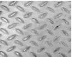
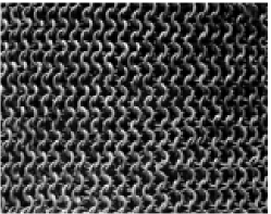
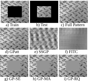
We extrapolate the missing region, shown in Figure 1a, on a real metal tread plate texture. There are 12675 training instances (Figure 1a), and 4225 test instances (Figure 1b). The inputs are pixel locations $x\in\mathbb{R}^{2}$ ($P=2$), and the outputs are pixel intensities. The full pattern is shown in Figure 1c. This texture contains shadows and subtle irregularities, no two identical diagonal markings, and patterns that have correlations across both input dimensions.

To reconstruct the missing region, as well as the training region, we use GPatt with $30$ components for the SMP kernel of Eq. (14) in each dimension (GPatt-30). The GPatt reconstruction shown in Figure 1d is as plausible as the true full pattern shown in Figure 1c, and largely automatic. Without human intervention – no hand crafting of kernel features to suit this image, no sophisticated initialisation, and no exposure to similar images – GPatt has discovered the underlying structure of this image and extrapolated that structure across a large missing region, even though the structure of this pattern is not independent across the two spatial input dimensions. Indeed the separability of the SMP kernel represents only a soft prior assumption, and does not rule out posterior correlations between input dimensions.

The reconstruction in Figure 1e was produced with SSGP, using 500 basis functions. In principle SSGP can model any spectral density (and thus any stationary kernel) with infinitely many components (basis functions). However, since these components are point masses (in frequency space), each component has highly limited expressive power. Moreover, with many components SSGP experiences practical difficulties regarding initialisation, over-fitting, and computation time (scaling quadratically with the number of basis functions). Although SSGP does discover some interesting structure (a diagonal pattern), and has equal training and test performance, it is unable to capture enough information for a convincing reconstruction, and we did not find that more basis functions improved performance. Likewise, FITC with an SMP-30 kernel and 500 pseudo-inputs cannot capture the necessary information to interpolate or extrapolate. We note FITC and SSGP-500 respectively took 2 days and 1 hour to run on this example, compared to GPatt which took under 5 minutes.

GPs with SE, MA, and RQ kernels are all truly Bayesian nonparametric models – these kernels are derived from infinite basis function expansions. Therefore, as seen in Figure 1 g), h), i), these methods are completely able to capture the information in the training region; however, these kernels do not have the proper structure to reasonably extrapolate across the missing region – they simply act as smoothing filters. We note that this comparison is only possible because these GPs are using the fast exact inference techniques in Section 4.

Overall, these results indicate that both expressive nonparametric kernels, such as the SMP kernel, and the specific fast inference in Section 4, are needed to be able to extrapolate patterns in these images.

Figure 1: Extrapolation on a Metal Tread Plate Pattern. Missing data are shown in black. a) Training region (12675 points), b) Testing region (4225 points), c) Full tread plate pattern, d) GPatt-30, e) SSGP with 500 basis functions, f) FITC with 500 pseudo inputs, and the SMP-30 kernel, and GPs with the fast exact inference in Section 4.1, and g) squared exponential (SE), h) Matérn (MA), and i) rational quadratic (RQ) kernels.

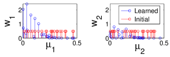
We note that the SMP-30 kernel used with GPatt has more components than needed for this problem. However, as shown in Figure 2, if the model is overspecified, the complexity penalty in the marginal likelihood shrinks the weights ($\{w_{a}\}$ in Eq. (13)) of extraneous components, as a proxy for model selection – an effect similar to automatic relevance determination (MacKay, 1994). As per Eq. (18), this complexity penalty can be written as a sum of eigenvalues of a covariance matrix $K$. Components which do not significantly contribute to model fit will therefore be automatically pruned, as shrinking the weights decreases the eigenvalues of $K$ and thus minimizes the complexity penalty. This weight shrinking helps mitigate the effects of model overspecification and helps indicate whether the model is overspecified. In the following stress tests we find that GPatt scales efficiently with the number of components in its SMP kernel.

Figure 2: Automatic Model Selection in GPatt. Initial and learned weight and frequency parameters of GPatt-30, for each input dimension (a dimension is represented in each panel), on the metal tread plate pattern of Figure 1. GPatt-30 is overspecified for this pattern. During training, weights of extraneous components automatically shrink to zero, which helps indicate whether the model is overspecified, and helps mitigate the effects of model overspecification. Of the 30 initial components in each dimension, 15 are near zero after training.

5.2 Stress Tests

We stress test GPatt and alternative methods in terms of speed and accuracy, with varying datasizes, extrapolation ranges, basis functions, pseudo inputs, and components. We assess accuracy using standardised mean square error (SMSE) and mean standardized log loss (MSLL) (a scaled negative log likelihood), as defined in Rasmussen & Williams (2006) on page 23. Using the empirical mean and variance to fit the data would give an SMSE and MSLL of 1 and 0 respectively. Smaller SMSE and more negative MSLL values correspond to better fits of the data.

The runtime stress test in Figure 3a shows that the number of components used in GPatt does not significantly affect runtime, and that GPatt is much faster than FITC (using 500 pseudo inputs) and SSGP (using 90 or 500 basis functions), even with $100$ components ($601$ kernel hyperparameters). The slope of each curve roughly indicates the asymptotic scaling of each method. In this experiment, the standard GP (with SE kernel) has a slope of $2.9$, which is close to the cubic scaling we expect. All other curves have a slope of $1\pm 0.1$, indicating linear scaling with the number of training instances. However, FITC and SSGP are used here with a fixed number of pseudo inputs and basis functions. More pseudo inputs and basis functions should be used when there are more training instances – and these methods scale quadratically with pseudo inputs and basis functions for a fixed number of training instances. GPatt, on the other hand, can scale linearly in runtime as a function of training size, without any deterioration in performance. Furthermore, the big gaps between each curve – the fixed 1-2 orders of magnitude GPatt outperforms alternatives – is as practically important as asymptotic scaling.

Figure 3: Stress Tests. a) Runtime Stress Test. We show the runtimes in seconds, as a function of training instances, for evaluating the log marginal likelihood, and any relevant derivatives, for a standard GP with SE kernel (as implemented in GPML), FITC with 500 pseudo-inputs and SMP-25 and SMP-5 kernels, SSGP with 90 and 500 basis functions, and GPatt-100, GPatt-25, and GPatt-5. Runtimes are for a 64bit PC, with 8GB RAM and a 2.8 GHz Intel i7 processor, on the cone pattern ($P=2$), shown in the Appendix. The ratio of training inputs to the sum of imaginary and training inputs for GPatt (Section 4.2) is $0.4$ and $0.6$ for the smallest two training sizes, and $0.7$ for all other training sets. b) Accuracy Stress Test. MSLL as a function of holesize on the metal pattern of Figure 1. The values on the horizontal axis represent the fraction of missing (testing) data from the full pattern (for comparison Fig 1a has 25% missing data). We compare GPatt-30 and GPatt-15 with GPs with SE, MA, and RQ kernels (and the inference of Section 4), and SSGP with $100$ basis functions. The MSLL for GPatt-15 at a holesize of $0.01$ is $-1.5886$.

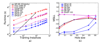
The accuracy stress test in Figure 3b shows extrapolation (MSLL) performance on the metal tread plate pattern of Figure 1c with varying holesizes, running from 0% to 60% missing data for testing (for comparison the hole shown in Figure 1a is for 25% missing data). GPs with SE, RQ, and MA kernels (and the fast inference of Section 4) all steadily increase in error as a function of holesize. Conversely, SSGP does not increase in error as a function of holesize – with finite basis functions SSGP cannot extract as much information from larger datasets as the alternatives. GPatt performs well relative to the other methods, even with a small number of components. GPatt is particularly able to exploit the extra information in additional training instances: only when the holesize is so large that over 60% of the data are missing does GPatt’s performance degrade to the same level as alternative methods.

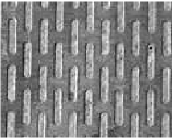
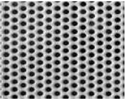
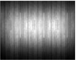
In Table 1 we compare the test performance of GPatt with SSGP, and GPs using SE, MA, and RQ kernels, for extrapolating five different patterns, with the same train test split as for the tread plate pattern in Figure 1. All patterns are shown in the Appendix. GPatt consistently has the lowest standardized mean squared error (SMSE), and mean standardized log loss (MSLL). Note that many of these datasets are sophisticated patterns, containing intricate details and subtleties which are not strictly periodic, such as lighting irregularities, metal impurities, etc. Indeed SSGP has a periodic kernel (unlike the SMP kernel which is not strictly periodic), and is capable of modelling multiple periodic components, but does not perform as well as GPatt on these examples.

Table 1: We compare the test performance of GPatt-30 with SSGP (using 100 basis functions), and GPs using squared exponential (SE), Matérn (MA), and rational quadratic (RQ) kernels, combined with the inference of Section 5.2, on patterns with a train test split as in the metal treadplate pattern of Figure 1.

	GPatt	SSGP	SE	MA	RQ
Rubber mat     (train = 12675, test = 4225)
SMSE	${\boldsymbol{\mathbf{0.31}}}$	$0.65$	$0.97$	$0.86$	$0.89$
MSLL	${\boldsymbol{\mathbf{-0.57}}}$	$-0.21$	$0.14$	$-0.069$	$0.039$
Tread plate      (train = 12675, test = 4225)
SMSE	${\boldsymbol{\mathbf{0.45}}}$	$1.06$	$0.895$	$0.881$	$0.896$
MSLL	${\boldsymbol{\mathbf{-0.38}}}$	$0.018$	$-0.101$	$-0.1$	$-0.101$
Pores        (train = 12675, test = 4225)
SMSE	${\boldsymbol{\mathbf{0.0038}}}$	$1.04$	$0.89$	$0.88$	$0.88$
MSLL	${\boldsymbol{\mathbf{-2.8}}}$	$-0.024$	$-0.021$	$-0.024$	$-0.048$
Wood        (train = 14259, test = 4941)
SMSE	${\boldsymbol{\mathbf{0.015}}}$	$0.19$	$0.64$	$0.43$	$0.77$
MSLL	${\boldsymbol{\mathbf{-1.4}}}$	$-0.80$	$1.6$	$1.6$	$0.77$
Chain mail     (train = 14101, test = 4779)
SMSE	${\boldsymbol{\mathbf{0.79}}}$	$1.1$	$1.1$	$0.99$	$0.97$
MSLL	${\boldsymbol{\mathbf{-0.052}}}$	$0.036$	$1.6$	$0.26$	$-0.0025$

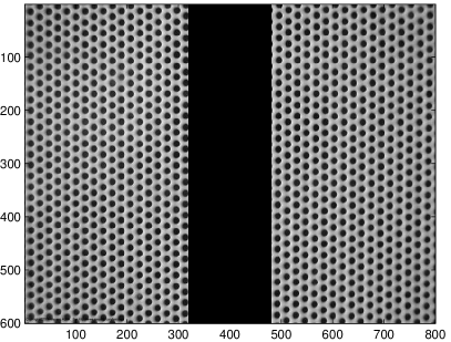
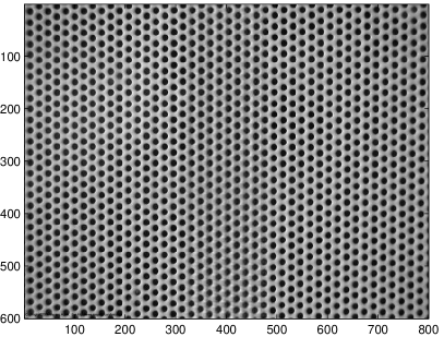
We end this Section with a particularly large example, where we use GPatt-10 to perform learning and exact inference on the Pores pattern, with $383400$ training points, to extrapolate a large missing region with $96600$ test points. The SMSE is $0.077$, and the total runtime was $2800$ seconds. Images of the successful extrapolation are shown in the Appendix.

5.3 Recovering Complex 3D Kernels from a Video

With a relatively small number of components, GPatt is able to accurately recover a wide range of product kernels. To test GPatt’s ability to recover ground truth kernels, we simulate a $50\times 50\times 50$ movie of data (e.g.  two spatial input dimensions, one temporal) using a GP with kernel $k=k_{1}k_{2}k_{3}$ (each component kernel in this product operates on a different input dimension), where $k_{1}=k_{\text{SE}}+k_{\text{SE}}\times k_{\text{PER}}$, $k_{2}=k_{\text{MA}}\times k_{\text{PER}}+k_{\text{MA}}\times k_{\text{PER}}$, and $k_{3}=(k_{\text{RQ}}+k_{\text{PER}})\times k_{\text{PER}}+k_{\text{SE}}$. ($k_{\text{PER}}(\tau)=\exp[-2\sin^{2}(\pi\,\tau\,\omega)/\ell^{2}]$, $\tau=x-x^{\prime}$). We use $5$ consecutive $50\times 50$ slices for testing, leaving a large number $N=112500$ of training points. In this case, the big datasize is helpful: the more training instances, the more information to learn the true generating kernels. Moreover, GPatt-20 is able to reconstruct these complex out of class kernels in under $10$ minutes. We compare the learned SMP-20 kernel with the true generating kernels in Figure 4. In the Appendix, we show true and predicted frames from the movie.

Figure 4: Recovering sophisticated product kernels. A product of three kernels (shown in green) was used to generate a movie of 112500 3D training points. From this data, GPatt-20 reconstructs these component kernels (the learned SMP-20 kernel is shown in blue). All kernels are a function of $\tau=x-x^{\prime}$. For clarity of presentation, each kernel has been scaled by $k(0)$.

5.4 Wallpaper and Scene Reconstruction

Figure 5: Image inpainting with GPatt. From left to right: A mask is applied to the original image, GPatt extrapolates the mask region in each of the three (red, blue, green) image channels, and the results are joined to produce the restored image. Top row: Removing a stain (train: $15047\times 3$). Bottom row: Removing a rooftop to restore a natural scene (train: $32269\times 3$). The coast is masked during training and we do not attempt to extrapolate it in testing.

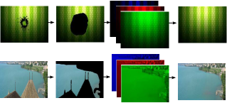
Although GPatt is a general purpose regression method, it can also be used for inpainting: image restoration, object removal, etc.

We first consider a wallpaper image stained by a black apple mark, shown in the first row of Figure 5. To remove the stain, we apply a mask and then separate the image into its three channels (red, green, and blue). This results in $15047$ pixels in each channel for training. In each channel we ran GPatt using SMP-30. We then combined the results from each channel to restore the image without any stain, which is particularly impressive given the subtleties in the pattern and lighting.

In our next example, we wish to reconstruct a natural scene obscured by a prominent rooftop, shown in the second row of Figure 5. By applying a mask, and following the same procedure as for the stain, this time with $32269$ pixels in each channel for training, GPatt reconstructs the scene without the rooftop. This reconstruction captures subtle details, such as waves in the ocean, even though only one image was used for training. In fact this example has been used with inpainting algorithms which were given access to a repository of thousands of similar images (Hays & Efros, 2008). The results emphasized that conventional inpainting algorithms and GPatt have profoundly different objectives, which are sometimes even at cross purposes: inpainting attempts to make the image look good to a human (e.g., the example in Hays & Efros (2008) placed boats in the water), while GPatt is a general purpose regression algorithm, which simply aims to make accurate predictions at test input locations, from training data alone.

6 Discussion

Gaussian processes are often used for smoothing and interpolation on small datasets. However, we believe that Bayesian nonparametric models are naturally suited to pattern extrapolation on large multidimensional datasets, where extra training instances can provide extra opportunities to learn additional structure in data.

The support and inductive biases of a Gaussian process are naturally encoded in a covariance kernel. A covariance kernel must always have some structure to reflect these inductive biases; and that structure can, in principle, be exploited for scalable and exact inference, without the need for simplifying approximations. Such models could play a role in a new era of machine learning, where models are expressive and scalable, but also interpretable and manageable, with simple exact learning and inference procedures.

We hope to make a small step in this direction with GPatt, a Gaussian process based Bayesian nonparametric framework for automatic pattern discovery on large multidimensional datasets, with scalable and exact inference procedures. Without human intervention – no sophisticated initialisation, or hand crafting of kernel features – GPatt has been used to accurately and quickly extrapolate large missing regions on a variety of patterns.

Acknowledgements: We thank Richard E. Turner, Ryan Prescott Adams, Zoubin Ghahramani, and Carl Edward Rasmussen for helpful discussions.

7 Appendix

7.1 Introduction

We provide further detail about the eigendecomposition of kronecker matrices, and the runtime complexity of kronecker matrix vector products. We also provide spectral images of the learned kernels in the metal tread plate experiment of Section 5.1, larger versions of the images in Table 1, images of the extrapolation results on the large pore example, and images of the GPatt reconstruction for several consecutive movie frames.

7.2 Eigendecomposition of Kronecker Matrices

Assuming a product kernel,

$$k(x_{i},x_{j})=\prod_{p=1}^{P}k^{p}(x_{i}^{p},x_{j}^{p})\,,$$ (24)

and inputs $x\in\mathcal{X}$ on a multidimensional grid, $\mathcal{X}=\mathcal{X}_{1}\times\dots\times\mathcal{X}_{P}\subset\mathbb{R}^{P}$, then the covariance matrix $K$ decomposes into a Kronecker product of matrices over each input dimension $K=K^{1}\otimes\dots\otimes K^{P}$ (Saatchi, 2011). The eigendecomposition of $K$ into $QVQ^{\top}$ similarly decomposes: $Q=Q^{1}\otimes\dots\otimes Q^{P}$ and $V=V^{1}\otimes\dots\otimes V^{P}$. Each covariance matrix $K^{p}$ in the Kronecker product has entries $K^{p}_{ij}=k^{p}(x_{i}^{p},x_{j}^{p})$ and decomposes as $K^{p}=Q^{p}V^{p}{Q^{p}}^{\top}$. Thus the $N\times N$ covariance matrix $K$ can be stored in $\mathcal{O}(PN^{\frac{2}{P}})$ and decomposed into $QVQ^{\top}$ in $\mathcal{O}(PN^{\frac{3}{P}})$ operations, for $N$ datapoints and $P$ input dimensions.

7.3 Matrix-vector Product for Kronecker Matrices

We first define a few operators from standard Kronecker literature. Let ${\boldsymbol{\mathbf{B}}}$ be a matrix of size $p\times q$. The ${\rm reshape}({\boldsymbol{\mathbf{B}}},r,c)$ operator returns a r-by-c matrix ($rc=pq$) whose elements are taken column-wise from ${\boldsymbol{\mathbf{B}}}$. The ${\rm vec}(\cdot)$ operator stacks the matrix columns onto a single vector, ${\rm vec}({\boldsymbol{\mathbf{B}}})={\rm reshape}({\boldsymbol{\mathbf{B}}},pq,1)$, and the ${\rm vec}^{-1}(\cdot)$ operator is defined as ${\rm vec}^{-1}({\rm vec}({\boldsymbol{\mathbf{{\boldsymbol{\mathbf{B}}}}}}))={\boldsymbol{\mathbf{B}}}$. Finally, using the standard Kronecker property $({\boldsymbol{\mathbf{B}}}\otimes{\boldsymbol{\mathbf{C}}}){\rm vec}({\boldsymbol{\mathbf{X}}})={\rm vec}({\boldsymbol{\mathbf{C}}}{\boldsymbol{\mathbf{X}}}{\boldsymbol{\mathbf{B}}}^{\top})$, we note that for any $N$ argument vector ${\boldsymbol{\mathbf{u}}}\in\mathbb{R}^{N}$ we have

$${\boldsymbol{\mathbf{K}}}_{N}{\boldsymbol{\mathbf{u}}} =\left(\bigotimes_{p=1}^{P}{\boldsymbol{\mathbf{K}}}^{p}_{N^{1/P}}\right){\boldsymbol{\mathbf{u}}}={\rm vec}\left({\boldsymbol{\mathbf{K}}}^{P}_{N^{1/P}}{\boldsymbol{\mathbf{U}}}\left(\bigotimes_{p=1}^{P-1}{\boldsymbol{\mathbf{K}}}^{p}_{N^{1/P}}\right)^{\top}\right),$$ (25)

where ${\boldsymbol{\mathbf{U}}}={\rm reshape}({\boldsymbol{\mathbf{u}}},N^{1/P},N^{\frac{P-1}{P}})$, and ${\boldsymbol{\mathbf{K}}}_{N}$ is an $N\times N$ Kronecker matrix. With no change to Eq. (25) we can introduce the ${\rm vec}^{-1}({\rm vec}(\cdot))$ operators to get

$${\boldsymbol{\mathbf{K}}}_{N}{\boldsymbol{\mathbf{u}}}={\rm vec}\left(\left(~{}~{}~{}{\rm vec}^{-1}\left({\rm vec}\left(~{}~{}~{}\left(\bigotimes_{p=1}^{P-1}{\boldsymbol{\mathbf{K}}}^{p}_{N^{1/P}}\right)\left({\boldsymbol{\mathbf{K}}}^{P}_{N^{1/P}}{\boldsymbol{\mathbf{U}}}\right)^{\top}~{}~{}~{}\right)\right)~{}~{}~{}\right)^{\top}\right).$$ (26)

The inner component of Eq. (26) can be written as

$${\rm vec}\left(\left(\bigotimes_{p=1}^{P-1}{\boldsymbol{\mathbf{K}}}^{p}_{N^{1/P}}\right)\left({\boldsymbol{\mathbf{K}}}^{P}_{N^{1/P}}{\boldsymbol{\mathbf{U}}}\right)^{\top}{\boldsymbol{\mathbf{I}}}_{N^{{1}/{P}}}\right)={\boldsymbol{\mathbf{I}}}_{N^{{1}/{P}}}\otimes\left(\bigotimes_{p=1}^{P-1}{\boldsymbol{\mathbf{K}}}^{p}_{N^{1/P}}\right){\rm vec}\left(\left({\boldsymbol{\mathbf{K}}}^{P}_{N^{1/P}}{\boldsymbol{\mathbf{U}}}\right)^{\top}\right).$$ (27)

Notice that Eq. (27) is in the same form as Eq. (25) (Kronecker matrix-vector product). By repeating Eqs. (26-27) over all $P$ dimensions, and noting that $\left(\bigotimes_{p=1}^{P}{\boldsymbol{\mathbf{I}}}_{N^{{1}/{P}}}\right){\boldsymbol{\mathbf{u}}}={\boldsymbol{\mathbf{u}}}$, we see that the original matrix-vector product can be written as

$$\left(\bigotimes_{p=1}^{P}{\boldsymbol{\mathbf{K}}}^{p}_{N^{1/P}}\right){\boldsymbol{\mathbf{u}}} =\operatorname{vec}\left(\left[{\boldsymbol{\mathbf{K}}}^{1}_{N^{1/P}},\dots\left[{\boldsymbol{\mathbf{K}}}^{P-1}_{N^{1/P}},\left[{\boldsymbol{\mathbf{K}}}^{P}_{N^{1/P}},{\boldsymbol{\mathbf{U}}}\right]\right]\right]\right)$$ (28)

$$\;{\buildrel\rm def\over{=}}\;{\rm kron\_mvprod}\left({\boldsymbol{\mathbf{K}}}^{1}_{N^{1/P}},{\boldsymbol{\mathbf{K}}}^{2}_{N^{1/P}},\dots,{\boldsymbol{\mathbf{K}}}^{P}_{N^{1/P}},{\boldsymbol{\mathbf{u}}}\right)$$ (29)

where the bracket notation denotes matrix product, transpose then reshape, i.e.,

$$\left[{\boldsymbol{\mathbf{K}}}^{p}_{N^{1/P}},{\boldsymbol{\mathbf{U}}}\right]={\rm reshape}\left(\left({\boldsymbol{\mathbf{K}}}^{p}_{N^{1/P}}{\boldsymbol{\mathbf{U}}}\right)^{\top},N^{1/P},N^{\frac{P-1}{P}}\right)\,.$$ (30)

Iteratively solving the ${\rm kron\_mvprod}$ operator in Eq. (29) requires $(PN^{\frac{P+1}{P}})$, because each of the $P$ bracket operations requires $\mathcal{O}(N^{\frac{P+1}{P}})$.

7.4 Inference with Imaginary Observations

The predictive mean of a Gaussian process at $L$ test points, given $N$ training points, is given by

$${\boldsymbol{\mathbf{\mu}}}_{L}={\boldsymbol{\mathbf{K}}}_{LN}\left({\boldsymbol{\mathbf{K}}}_{N}+\sigma^{2}I_{N}\right)^{-1}{\boldsymbol{\mathbf{y}}}\,,$$ (31)

where ${\boldsymbol{\mathbf{K}}}_{LN}$ is an $L\times N$ matrix of cross covariances between the test and training points. We wish to show that when we have $M$ observations which are not on a grid that the desired predictive mean

$${\boldsymbol{\mathbf{\mu}}}_{L}={\boldsymbol{\mathbf{K}}}_{LM}\left({\boldsymbol{\mathbf{K}}}_{M}+\sigma^{2}I_{M}\right)^{-1}{\boldsymbol{\mathbf{y}}}_{M}={\boldsymbol{\mathbf{K}}}_{LN}\left({\boldsymbol{\mathbf{K}}}_{N}+{\boldsymbol{\mathbf{D}}}_{N}\right)^{-1}{\boldsymbol{\mathbf{y}}}\,,$$ (32)

where ${\boldsymbol{\mathbf{y}}}=[{\boldsymbol{\mathbf{y}}}_{M},{\boldsymbol{\mathbf{y}}}_{W}]^{\top}$ includes imaginary observations ${\boldsymbol{\mathbf{y}}}_{W}$, and $D_{N}$ is as defined in Section 4. as

$${D}_{N}=\left[\begin{array}[]{cc}{D}_{M}&0\\ 0&{\epsilon}^{-1}{I}_{W}\end{array}\right],$$ (35)

where we set $D_{M}=\sigma^{2}I_{M}$.

Starting with the right hand side of Eq. (32),

$${\boldsymbol{\mathbf{\mu}}}_{L}=\left[\begin{array}[]{c}{\boldsymbol{\mathbf{K}}}_{LM}\\ {\boldsymbol{\mathbf{K}}}_{LW}\end{array}\right]\left[\begin{array}[]{cc}{\boldsymbol{\mathbf{K}}}_{M}+{\boldsymbol{\mathbf{D}}}_{M}&{\boldsymbol{\mathbf{K}}}_{MW}\\ {\boldsymbol{\mathbf{K}}}_{MW}^{\top}&{\boldsymbol{\mathbf{K}}}_{W}+{\epsilon}^{-1}{\boldsymbol{\mathbf{I}}}_{W}\end{array}\right]^{-1}\left[\begin{array}[]{c}{\boldsymbol{\mathbf{y}}}_{M}\\ {\boldsymbol{\mathbf{y}}}_{W}\end{array}\right].\\$$ (36)

Using the block matrix inversion theorem, we get

$$\left[\begin{array}[]{cc}A&B\\ C&E\end{array}\right]^{-1}=\left[\begin{array}[]{cc}(A-BE^{-1}C)^{-1}&-A^{-1}B(I-E^{-1}CA^{-1}B)^{-1}E^{-1}\\ -E^{-1}C(A-BE^{-1}C)^{-1}&(I-E^{-1}CA^{-1}B)^{-1}E^{-1}\end{array}\right],$$ (41)

where $A={\boldsymbol{\mathbf{K}}}_{M}+{\boldsymbol{\mathbf{D}}}_{M}$, $B={\boldsymbol{\mathbf{K}}}_{MW}$, $C={\boldsymbol{\mathbf{K}}}_{MW}^{\top}$, and $E={\boldsymbol{\mathbf{K}}}_{W}+{\epsilon}^{-1}{\boldsymbol{\mathbf{I}}}_{W}$. If we take the limit of $E^{-1}={\epsilon}(\epsilon{\boldsymbol{\mathbf{K}}}_{W}+{\boldsymbol{\mathbf{I}}}_{W})^{-1}\buildrel\epsilon\rightarrow 0\over{\longrightarrow}{\boldsymbol{\mathbf{0}}}$, and solve for the other components, Eq. (36) becomes

$${\boldsymbol{\mathbf{\mu}}}_{L} =\left[\begin{array}[]{c}{\boldsymbol{\mathbf{K}}}_{LM}\\ {\boldsymbol{\mathbf{K}}}_{LW}\end{array}\right]\left[\begin{array}[]{cc}\left({\boldsymbol{\mathbf{K}}}_{M}+{\boldsymbol{\mathbf{D}}}_{M}\right)^{-1}&{\boldsymbol{\mathbf{0}}}\\ {\boldsymbol{\mathbf{0}}}&{\boldsymbol{\mathbf{0}}}\end{array}\right]\left[\begin{array}[]{c}{\boldsymbol{\mathbf{y}}}_{M}\\ {\boldsymbol{\mathbf{y}}}_{W}\end{array}\right]={\boldsymbol{\mathbf{K}}}_{LM}({\boldsymbol{\mathbf{K}}}_{M}+{\boldsymbol{\mathbf{D}}}_{M})^{-1}{\boldsymbol{\mathbf{y}}}_{M}$$ (48)

which is the exact GP result. In other words, performing inference given observations ${\boldsymbol{\mathbf{y}}}$ will give the same result as directly using observations ${\boldsymbol{\mathbf{y}}}_{M}$. The proof that the predictive covariances remain unchanged proceeds similarly.

7.5 Spectrum Analysis

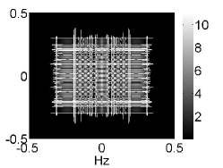
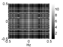
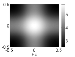
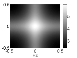
We can gain further insight into the behavior of GPatt by looking at the spectral density learned by the spectral mixture kernel. Figure 6 shows the log spectrum representations of the learned kernels from Section 5.1. Smoothers, such as the popular SE, RQ, and MA kernels concentrate their spectral energy around the origin, differing only by their tail support for higher frequencies. Methods which used the SMP kernel, such as the GPatt and FITC (with an SMP kernel), are able to learn meaningful features in the spectrum space.

(a) GPatt-30

(b) FITC

(c) SE

(d) RQ

(e) MA

Figure 6: Spectral representation of the learned kernels from Section 5.1. For methods which used the SMP kernel (namely, a) GPatt and b) FITC) we plot the analytical log spectrum using the learned hyperparameters. For c)Squared exponential, d) Rational quadratic, and e) Matérn-3 we plot instead the empirical log spectrum using the Fast Fourier transform of the kernel.

7.6 Images

In the rest of the supplementary material, we provide the images and results referenced in the main text. Figure 7 illustrates the images used for the stress tests in Section 5.2. In Figure 8, we provide the results for the large pore example. Finally, Figure 9 shows the true and predicted movie frames discussed in Section 5.3.

(a) Rubber mat

(b) Tread plate

(c) Pores

(d) Wood

(e) Chain mail

(f) Cone

Figure 7: Images used for stress tests in Section 5.2. Figures a) through e) show the textures used in the accuracy comparison of Table 1. Figure e) is the cone image which was used for the runtime analysis shown in Figure 3a.

(a) Train

(b) Learn

Figure 8: GPatt on a particularly large multidimensional dataset. a) Training region (383400 points), b) GPatt-10 reconstruction of the missing region.

Figure 9: Using GPatt to recover 5 consecutive slices from a movie. All slices are missing from training data (e.g., these are not 1 step ahead forecasts). Top row: true slices take from the middle of the movie. Bottom row: inferred slices using GPatt-20.

References

- Atkinson (2008) Atkinson, Kendall E. An introduction to numerical analysis. John Wiley & Sons, 2008.
- Bochner (1959) Bochner, S. Lectures on Fourier Integrals.(AM-42), volume 42. Princeton University Press, 1959.
- Duvenaud et al. (2013) Duvenaud, D., Lloyd, J.R., Grosse, R., Tenenbaum, J.B., and Ghahramani, Z. Structure discovery in nonparametric regression through compositional kernel search. In International Conference on Machine Learning, 2013.
- Ghahramani (2012) Ghahramani, Z. Bayesian nonparametrics and the probabilistic approach to modelling. Philosophical Transactions of the Royal Society A, 2012.
- Gönen & Alpaydın (2011) Gönen, M. and Alpaydın, E. Multiple kernel learning algorithms. Journal of Machine Learning Research, 12:2211–2268, 2011.
- Hays & Efros (2008) Hays, J and Efros, A. Scene completion using millions of photographs. Communications of the ACM, 51(10):87–94, 2008.
- Hensman et al. (2013) Hensman, J, Fusi, N, and Lawrence, N.D. Gaussian processes for big data. In Uncertainty in Artificial Intelligence (UAI). AUAI Press, 2013.
- Hörmander (1990) Hörmander, L. The Analysis of Linear Partial Differential Operators I, Distribution Theory and Fourier Analysis. Springer-Verlag, 1990.
- Kostantinos (2000) Kostantinos, N. Gaussian mixtures and their applications to signal processing. Advanced Signal Processing Handbook: Theory and Implementation for Radar, Sonar, and Medical Imaging Real Time Systems, 2000.
- Krizhevsky et al. (2012) Krizhevsky, A., Sutskever, I, and Hinton, G. Imagenet classification with deep convolutional neural networks. In Advances in Neural Information Processing Systems, 2012.
- Lázaro-Gredilla et al. (2010) Lázaro-Gredilla, M., Quiñonero-Candela, J., Rasmussen, C.E., and Figueiras-Vidal, A.R. Sparse spectrum gaussian process regression. The Journal of Machine Learning Research, 11:1865–1881, 2010.
- Le et al. (2013) Le, Q., Sarlos, T., and Smola, A. Fastfood-computing hilbert space expansions in loglinear time. In Proceedings of the 30th International Conference on Machine Learning, pp. 244–252, 2013.
- MacKay (1998) MacKay, David J.C. Introduction to Gaussian processes. In Christopher M. Bishop, editor (ed.), Neural Networks and Machine Learning, chapter 11, pp. 133–165. Springer-Verlag, 1998.
- MacKay (1994) MacKay, D.J.C. Bayesian nonlinear modeling for the prediction competition. Ashrae Transactions, 100(2):1053–1062, 1994.
- Murray & Adams (2010) Murray, I. and Adams, R.P. Slice sampling covariance hyperparameters in latent Gaussian models. In Advances in Neural Information Processing Systems, 2010.
- Naish-Guzman & Holden (2007) Naish-Guzman, A and Holden, S. The generalized fitc approximation. In Advances in Neural Information Processing Systems, pp. 1057–1064, 2007.
- Neal (1996) Neal, R.M. Bayesian Learning for Neural Networks. Springer Verlag, 1996. ISBN 0387947248.
- Quiñonero-Candela & Rasmussen (2005) Quiñonero-Candela, J. and Rasmussen, C.E. A unifying view of sparse approximate gaussian process regression. The Journal of Machine Learning Research, 6:1939–1959, 2005.
- Rahimi & Recht (2007) Rahimi, A and Recht, B. Random features for large-scale kernel machines. In In Neural Information Processing Systems, 2007.
- Rasmussen (1996) Rasmussen, C.E. Evaluation of Gaussian Processes and Other Methods for Non-linear Regression. PhD thesis, University of Toronto, 1996.
- Rasmussen & Ghahramani (2001) Rasmussen, C.E. and Ghahramani, Z. Occam’s razor. In Neural Information Process Systems, 2001.
- Rasmussen & Williams (2006) Rasmussen, C.E. and Williams, C.K.I. Gaussian processes for Machine Learning. The MIT Press, 2006.
- Rumelhart et al. (1986) Rumelhart, D.E., Hinton, G.E., and Williams, R.J. Learning representations by back-propagating errors. Nature, 323(6088):533–536, 1986.
- Saatchi (2011) Saatchi, Y. Scalable Inference for Structured Gaussian Process Models. PhD thesis, University of Cambridge, 2011.
- Seeger et al. (2003) Seeger, M., Williams, C.K.I., and Lawrence, N.D. Fast forward selection to speed up sparse gaussian process regression. In Workshop on AI and Statistics, volume 9, pp. 2003, 2003.
- Snelson & Ghahramani (2006) Snelson, E. and Ghahramani, Z. Sparse gaussian processes using pseudo-inputs. In Advances in neural information processing systems, volume 18, pp. 1257. MIT Press, 2006.
- West (2013) West, G. Big Data Needs a Big Theory to Go with It. Scientific American, May 2013.
- Williams & Seeger (2001) Williams, C and Seeger, M. Using the nyström method to speed up kernel machines. In Advances in Neural Information Processing Systems, pp. 682–688. MIT Press, 2001.
- Wilson & Adams (2013) Wilson, A.G. and Adams, R.P. Gaussian process kernels for pattern discovery and extrapolation. International Conference on Machine Learning, 2013.