Efficient and Robust Allocation Algorithms in Clouds under Memory Constraints

Abstract

We consider robust resource allocation of services in Clouds. More specifically, we consider the case of a large public or private Cloud platform that runs a relatively small set of large and independent services. These services are characterized by their demand along several dimensions (CPU, memory,$\dots$) and by their quality of service requirements, that have been defined through an SLA in the case of a public Cloud or fixed by the administrator in the case of a private Cloud. This quality of service defines the required robustness of the service, by setting an upper limit on the probability that the provider fails to allocate the required quantity of resources. This maximum probability of failure can be transparently turned into a pair $(price,penalty)$. Failures can indeed hit the platform, and resilience is provided through service replication.

Our contribution is two-fold. Firstly, we propose a resource allocation strategy whose complexity is logarithmic in the number of resources, what makes it very efficient for large platforms. Secondly, we propose an efficient algorithm based on rare events detection techniques in order to estimate the robustness of an allocation, a problem that has been proven to be #P-complete. Finally, we provide an analysis of the proposed strategy through an extensive set of simulations, both in terms of the overall number of allocated resources and in terms of time necessary to compute the allocation.

Keywords: Cloud; reliability; failure; service; allocation; bin packing; linear program; memory; CPU; column generation; large scale; probability estimate; replication; resilience;

1 Introduction

Recently, there has been a dramatic change in both the platforms and the applications used in parallel processing. On the one hand, there has been a dramatic scale change, that is expected to continue both in data centers and in exascale machines. On the other hand, a dramatic simplification change has also occurred in the application models and scheduling algorithms. On the application side, many large scale applications are expressed as (sequences of) independent tasks, such as MapReduce [1, 2, 3] applications or even run as independent services handling requests.

In fact, the main reason behind this paradigm shift is not related to scale but rather to unpredictability. First of all, estimating the duration of a task or the time of a data transfer is extremely difficult, because of NUMA effects, shared platforms, complicating network topologies and the number of concurrent computations/transfers. Moreover, given the number of involved resources, failures are expected to happen at a frequency such that robustness to failures is a crucial issue for large scale applications running on Cloud platforms. In this context, the cost of purely runtime solutions, agnostic to the application and based either on checkpointing strategies [4, 5, 6] or application replication [7, 8] is expected to be large, and there is a clear interest for application-level solutions that take the inner structure of the application to enforce fault-tolerance.

In this paper, we will consider reliability issues in a very simple context, although representative of many Cloud applications. More specifically, we will consider the problems that arise when allocating independent services running as Virtual Machines (VMs) onto Physical Machines (PMs) in a Cloud Computing platform [9, 10]. The platforms that we target have a few crucial properties. First, we assume that the platform itself is very large, in terms of number of physical machines. Secondly, we assume that the set of services running on this platform is relatively small, and that each service requires a large number of resources. Therefore, our assumptions corresponds well to a datacenter or a large private Cloud such as those presented in [11], but not at all to a Cloud such as Amazon EC2 [12] running a huge number of small applications.

In the static case, mapping VMs with heterogeneous computing demands onto PMs with capacities is amenable to a multi-dimensional bin-packing problem (each dimension corresponding to a different kind of resource, memory, CPU, disk, bandwidth,$\dots$). Indeed, in this context, on the Cloud administrator side, each physical machine comes with its computing capacity (i.e. the number of flops it can process during one time-unit), its disk capacity (i.e. the number of bytes it can read/write during one time-unit), its network capacity (i.e. the number of bytes it can send/receive during one time-unit), its memory capacity (given that each VM comes with its complete software stack) and its failure rate (i.e. the probability that the machine will fail during the next time period). On the client side, each service comes with its requirement along the same dimensions (memory, CPU, disk and network footprints) and a reliability demand that has been negociated through an SLA [11].

In order to deal with resource allocation problems in Clouds, several sophisticated techniques have been developed in order to optimally allocate VMs onto PMs, either to achieve good load-balancing [13, 14, 15] or to minimize energy consumption [16, 17]. Most of the works in this domain have therefore focused on designing offline [18] and online [19, 20] solutions of Bin Packing variants.

In this paper, we propose to reformulate these heterogeneous resource allocation problems in a form that takes advantage on the assumptions we made on the platform and the characteristics of VMs. This set of assumption is crucial for the algorithms we propose. In this perspective, since we assume that the number of processing resources $m$ is very large, so that we will focus on resource allocation algorithms whose complexity is low (in practice logarithmic) in $m$. We also assume that each VM comes with its full software stack, so that the number of different services $K_{\max}$ that can actually run on the platform is very small, and will be treated as a small constant. We also assume that the number of services $\mathit{ns}$ is also small. Typically, we will propose algorithms that will rely on the partial enumeration of the possible configurations of a set of PMs (i.e. the set of applications they run) and more precisely on column generation techniques [21, 22] in order to solve efficiently the optimization problems. In Section 5, we will provide a detailed analysis of the resource allocation algorithm that we propose in this paper for a wide set of practical parameters. The cost of the algorithm will be analyzed both in terms of their processing time to find the allocation and in terms of the quality of the computed allocation (i.e. required number of resources).

Reliability constraints have received much less attention in the context of Cloud computing, as underlined by Cirne et al. [11]. Nevertheless, reliability issues have been addressed in more distributed and less reliable systems such as Peer-to-Peer networks. In such systems, efficient data sharing is complicated by erratic node failure, unreliable network connectivity and limited bandwidth. In this case, data replication can be used to improve both availability and response time and the question is to determine where to replicate data in order to meet simultaneously performance and availability requirements in large-scale systems [23, 24, 25, 26, 27]. Reliability issues have also been addressed by High Performance Computing community. Indeed, the exascale community [28, 29] underlines the importance of fault tolerance issues [30] and proposed solutions based either on replication strategies [8, 7] or rollback recovery relying on checkpointing protocols [4, 5, 6].

This work is a follow-up of [31], where the question of how to evaluate the reliability of an allocation has been addressed. One of the main results of [31] was that estimating the reliability of a given allocation was already a #P-complete problem [32, 33, 34]. In this paper, we prove that rare event detection techniques [35] developed by the Applied Probability community are in fact extremely efficient in practice to circumvent this complexity result. This paper is also a follow-up of [36], where asymptotically approximation algorithms for energy minimization have been proposed in the context where services were defined by their processing requirement only (and not their memory requirement). In [36], approximation techniques to estimate the reliability of an allocation were based on the use of Chernoff [37] and Hoeffding [38] bounds. In the present paper, we propose different techniques based on the approximation of the binomial distribution by the Gaussian distribution.

The paper is organized as follows. In Section 2, we present the notations that will be used throughout this paper and we define the characteristics of both the platform and the services that are suitable for the techniques we propose. In Section 3, we propose an algorithm for solving the resource allocation problem under reliability constraints. It relies on a pre-processing phase that is used to decompose the problem into a reliability problem and a packing problem. In Section 4, we propose a new technique based on rare event detection techniques to estimate the reliability of an allocation, and we prove that this technique is very efficient in our context. At last, we present in Section 5 a set of detailed simulation results that enable to analyze the performance of the algorithm proposed in Section 3 both in terms of the quality of returned allocations and processing time. Concluding remarks are presented in Section 6.

2 Framework

2.1 Platform and services description

In this paper, we assume the following model. On the one hand, the platform is composed of $m$ homogeneous machines $\mathcal{M}_{1},\dots,\mathcal{M}_{m}$, that have the same CPU capacity $C$ and the same memory capacity $M$. On the other hand, we aim at running $\mathit{ns}$ services $\mathcal{S}_{1},\dots,\mathcal{S}_{\mathit{ns}}$, that come with their CPU and memory requirements. In this context, our goal is to minimize the number of used machines, and at to find an allocation of the services onto the machines such that all packing constraints are fulfilled. Nevertheless, this problem is not equivalent to a classical multi-dimensional packing problem. Indeed, the two requirements are of a different nature.

On the one hand, services are heterogeneous from a CPU perspective, hence each service $\mathcal{S}_{i}$ expects that it will be provided a total computation power of $d_{i}$ (called demand) among all the machines. In addition, CPU sharing is modeled in a fluid manner: on a given machine, the fraction of the total CPU dedicated to a given service can take any (rational) value. This expresses the fact that the sharing between services which are running on a given machine is done through time multiplexing, whose grain is very fine.

On the other hand, memory requirements are homogeneous among all services, and memory requirements cannot be partially allocated: running a service on a machine occupies one unit of memory of this machine, regardless of the amount of computation power allocated to this service. This assumption models the fact that most of the memory used by virtual machines comes from the complete software stack image that needs to be deployed. On the other hand, the homogeneous assumption is not a strong requirement, and our algorithms could be modified to account for heterogeneous memory requirements (at the price of more complex notations). Furthermore, since the complete software stack image is needed, we assume that the memory capacity of the machines is not very high, i.e. each machine can hold at most 10 services.

2.2 Failure model

In this paper, we envision large-scale platforms, which means that machine failures are not uncommon and need to be taken into account. Two techniques are usually set up to face those machine failures: migration and replication. The response time of migrations may be too high to ensure continuity of the services. Therefore, we concentrate in this paper on a phase that occurs between two migration and reallocation operations, that are scheduled every $x$ hours. The migration and reallocation strategy is out of the scope of this paper and we rather concentrate on the use of replication in order to provide the resilience between two migration phases. The SLA defines the robustness properties that the allocation should have.

More specifically, we assume that machine failures are independent, and that machines are homogeneous also with regard to failures. We denote $f$ the probability that a given machine fails during the time period between two migration phases. Because of those failures, we cannot ensure that a service will have enough computational power at its disposal during the whole time period. The probability that all machines in the platform fail is indeed positive. Therefore, in our model each service $\mathcal{S}_{i}$ is also described with its reliability requirement $r_{i}$, which expresses a constraint: the probability that the service has not enough computational power (less than its demand $d_{i}$) at the end of the time period must be lower than $r_{i}$.

In this context, replicating a given service of many machines whose failure are independent, it will be possible to achieve any reliability requirement. Our goal in this paper is to do it for all services simultaneously, i.e. to enforce that capacity constraints, reliability requirements and service demands will be satisfied, while minimizing the number of required machines.

subsectionProblem description

We are now ready to state precisely the problem. Let $A_{i,j}$ be the CPU allocated to service $\mathcal{S}_{i}$ on machine $\mathcal{M}_{j}$, for all $i\in\{1,\dots,\mathit{ns}\}$ and $j\in\{1,\dots,m\}$. For all $j\in\{1,\dots,m\}$, we denote $\mathit{is\_alive}_{j}$ the random variable which is equal to 1 if machine $\mathcal{M}_{j}$ is alive at the end of the time period, and 0 otherwise. We can then define, for all $i\in\{1,\dots,\mathit{ns}\}$, the total CPU amount that is available to service $\mathcal{S}_{i}$ at the end of the time period: $\mathit{Alive\_cpu}_{i}=\sum_{j=1}^{m}\mathit{is\_alive}_{j}\times A_{i,j}$. The problem of the minimization of the number of used machines can be written as:

$$\begin{array}[]{c}\mathrm{min}\\ m\\ \mathrm{s.t.}\end{array} \forall i,\mathbb{P}\left(\mathit{Alive\_cpu}_{i}<d_{i}\right)<r_{i}$$ (4)

$$\begin{array}[]{c}\mathrm{min}\\ m\\ \mathrm{s.t.}\end{array} \forall j,\mathit{card}\left\{A_{i,j}\neq 0\,;i\in\{1,\dots,\mathit{ns}\}\right\}\leq M$$ (8)

$$\begin{array}[]{c}\mathrm{min}\\ m\\ \mathrm{s.t.}\end{array} \forall j,\sum_{i=1}^{\mathit{ns}}A_{i,j}\leq C$$ (12)

Equations (8) and (12) depict the packing constraints, while Equation (4) deals with reliability requirements.

We will use in this paper two approaches for the estimation of the reliability requirements. In the No-Approx model, the reliability constraint is actually written $\mathbb{P}\left(\mathit{Alive\_cpu}_{i}<d_{i}\right)<r_{i}$.

However, as previously stated, given an allocation of one service onto the machines, deciding whether this allocation fulfills the reliability constraint or not is a #P-complete problem [31]; this shows that estimating this reliability constraint is a hard task. In [39], it has been observed that, based on the approximation of a binomial distribution by a Gaussian distribution, $\mathbb{P}\left(\mathit{Alive\_cpu}_{i}<d_{i}\right)<r_{i}$ is approximately equivalent to

$$\sum_{j=1}^{m}A_{i,j}-B_{i}\sqrt{\sum_{j=1}^{m}A_{i,j}^{2}}\geq K_{i},\mathrm{~{}~{}where}$$

$$K_{i}=\frac{d_{i}}{1-f}\quad\mathrm{and}\quad B_{i}=z_{r_{i}}\times\sqrt{\frac{f}{1-f}}.$$

$z_{r_{i}}$ is a characteristic of normal distributions, and only depends on $r_{i}$, therefore it can be tabulated beforehand. In the following, we will denote this model by the Normal-Approx model.

Both packing and fulfilling the reliability constraints are hard problems on their own, and it is even harder to deal with those two issues simultaneously. In the next section, we describe the way we solve the global problem, by decomposing it into two sub-problems that are easier to tackle.

3 Problem resolution

We approach the problem through a two-step heuristic. The first step focuses mainly on reliability issues. The general idea about reliability is that, for a given service, in order to keep the replication factor low (and thus reduce the total number of machines used), the service has to be divided into small slices and distributed among sufficiently many machines. However, using too many small slices for each service would break the memory constraints (remember that the memory requirement associated to a service is the same whatever the size of slice, as soon as it is larger than 0). The goal of the first step, described in Section 3.1, is thus to find reasonable slice sizes for each service, by using a relaxed packing formulation which can be solved optimally.

In a second step, described in Sections 3.2, we compute the actual packing of those service slices onto the machines. Since the number of different services allocated to each machine is expected to be low (because of the memory constraints), we rely on a formulation of the problem based on the partial enumeration of the possible configurations of machines, and we use column generation techniques [21, 22] to limit the number of different configurations.

3.1 Focus on reliability

In this section, we describe the first step of our approach: how to compute allocations that optimize the compromise between reliability and packing constraints, under both No-Approx and Normal-Approx models. This is done by considering a simpler, relaxed formulation of the problem, that can be solved optimally. We start with the Normal-Approx model.

3.1.1 Normal-Approx model

As stated before, in this first phase, we relax the problem by considering global capacities instead of capacities per machine. Thus we dispose of a total budget $mM$ for memory requirements and $mC$ for CPU needs, and use the following formulation:

$$\begin{array}[]{c}\mathrm{min}\\ m\\ \mathrm{s.t.}\end{array} \forall i,\sum_{j=1}^{m}A_{i,j}-B_{i}\sqrt{\sum_{j=1}^{m}A_{i,j}^{2}}\geq K_{i}$$ (16)

$$\begin{array}[]{c}\mathrm{min}\\ m\\ \mathrm{s.t.}\end{array} \sum_{j=1}^{m}\mathit{card}\left\{A_{i,j}\neq 0\,;i\in\{1,\dots,\mathit{ns}\}\right\}\leq mM$$ (20)

$$\begin{array}[]{c}\mathrm{min}\\ m\\ \mathrm{s.t.}\end{array} \sum_{j=1}^{m}\sum_{i=1}^{\mathit{ns}}A_{i,j}\leq mC$$ (24)

In the following, we prove that this formulation can be solved optimally. We define a class of solutions, namely homogeneous allocations, in which each service is allocated on a set of machines, with the same CPU requirement. Formally, an allocation is homogeneous if for all $i\in\{1,\dots,\mathit{ns}\}$, there exists $A_{i}$ such that for all $j\in\{1,\dots,m\}$, either $A_{i,j}=A_{i}$ or $A_{i,j}=0$.

Lemma 1.

On the relaxed problem, homogeneous allocations is a dominant class of solutions.

Proof.

Let us assume that there exist $i$, $j_{1}$ and $j_{2}\neq j_{1}$, such that $A_{i,j_{1}}>A_{i,j_{2}}>0$. By setting $A_{i,j_{1}}^{\prime}=A_{i,j_{2}}^{\prime}=(A_{i,j_{1}}+A_{i,j_{2}})/2$, we increase the left-hand side of Equation (16), and leave unchanged the left-hand sides of Equations (20) and (24). From any solution of the problem, we can build another homogeneous solution, which does not use a larger number of machines. ∎

An homogeneous allocation is defined by $n_{i}$, the number of machines hosting service $\mathcal{S}_{i}$, and $A_{i}$, the common CPU consumption of service $\mathcal{S}_{i}$ on each machine it is allocated to. The problem of finding an optimal homogeneous allocation can be written as:

$$\mathrm{min~{}}m\mathrm{~{}s.t.~{}} \forall i,n_{i}A_{i}-B_{i}A_{i}\sqrt{n_{i}}\geq K_{i}$$ (25)

$$\mathrm{min~{}}m\mathrm{~{}s.t.~{}} \forall i,A_{i}\geq 0$$

$$\mathrm{min~{}}m\mathrm{~{}s.t.~{}} \sum_{i}n_{i}\leq mM$$

$$\mathrm{min~{}}m\mathrm{~{}s.t.~{}} \sum_{i}n_{i}A_{i}\leq mC$$

which can be simplified into

$$\mathrm{min~{}}m\mathrm{~{}s.t.~{}}\quad\left\{\begin{array}[]{*1{>{\displaystyle}l}}\forall i,\sqrt{n_{i}}>B_{i}\\ \sum_{i}n_{i}\leq mM\\ \sum_{i}\frac{K_{i}}{1-\frac{B_{i}}{\sqrt{n_{i}}}}\leq mC\end{array}\right.$$ (26)

In the following, we search for a fractional solution to this problem: both $m$, the $n_{i}$’s and the $A_{i}$’s are assumed to be rational numbers. We begin by formulating two remarks to help solving this problem.

Remark 1.

We can restrict to solutions which satisfy the following constraints:

$$\forall i,\sqrt{n_{i}}>B_{i}$$

$$\sum_{i}n_{i}=mM$$

$$\sum_{i}\frac{K_{i}}{1-\frac{B_{i}}{\sqrt{n_{i}}}}=mC$$

Proof.

For all $i$, $\frac{K_{i}}{1-\frac{B_{i}}{\sqrt{n_{i}}}}$ is a non-increasing function of $n_{i}$, thus given a solution of Problem 26, we can build another solution such that $\sum_{i}n_{i}=mM$. Indeed, let $(n_{1},\dots,n_{\mathit{ns}})$ be an optimal solution of Problem 26, and let $n_{i}^{\prime}=n_{i}$ for all $i\in\{2,\dots,\mathit{ns}\}$. Now if we set $n_{1}^{\prime}=mM-\sum_{i=2}^{\mathit{ns}}n_{i}$, we have on the one hand $\sum_{i=1}^{\mathit{ns}}n_{i}^{\prime}=mM$, and on the other hand $\sum_{i=1}^{\mathit{ns}}\frac{K_{i}}{1-B_{i}/\sqrt{n_{i}^{\prime}}}\leq mC$, since $n_{1}^{\prime}\geq n_{1}$.

In the following, we only consider such solutions: let $(n_{1},\dots,n_{\mathit{ns}})$ be a solution of Problem 26 with $m$ machines, and satisfying $\sum_{i}n_{i}=mM$. Let us now further assume that, in this solution, $\sum_{i}\frac{K_{i}}{1-\frac{B_{i}}{\sqrt{n_{i}}}}<mC$. We show that such a solution is not optimal by exhibiting a valid solution $(n_{1}^{\prime},\dots,n_{\mathit{ns}}^{\prime})$, which uses $m^{\prime}<m$ machines. We set, for all $i\in\{2,\dots,\mathit{ns}\}$, $n_{i}^{\prime}=n_{i}$, and we define $n_{1}^{\prime}$ such that:

$$\sqrt{n_{1}^{\prime}}=\max\Bigg{(} \frac{\sqrt{n_{1}}+B_{1}}{2},$$

$$\frac{B_{1}}{1-\frac{2B_{1}}{mC-\sum_{i\neq 1}\frac{K_{i}}{1-B_{i}/\sqrt{n_{i}}}+\frac{K_{1}}{1-B_{1}/\sqrt{n_{1}}}}}\Bigg{)}.$$

We have firstly $\sqrt{n_{1}^{\prime}}\geq(\sqrt{n_{1}}+B_{1})/2>2B_{1}/2$, since $\sqrt{n_{1}}>B_{1}$. Furthermore, we prove now that $\sqrt{n_{1}^{\prime}}<\sqrt{n_{1}}$. On the one hand, again from $B_{1}<\sqrt{n_{1}}$, we obtain $(\sqrt{n_{1}}+B_{1})/2<\sqrt{n_{1}}$. On the other hand, from $\sum_{i}\frac{K_{i}}{1-\frac{B_{i}}{\sqrt{n_{i}}}}<mC$, we have

$$\frac{B_{1}}{1-\frac{2K_{1}}{mC-\sum_{i\neq 1}\frac{K_{i}}{1-B_{i}/\sqrt{n_{i}}}+\frac{K_{1}}{1-B_{1}/\sqrt{n_{1}}}}}<\sqrt{n_{1}}.$$

Finally $\sqrt{n_{1}^{\prime}}<\sqrt{n_{1}}$, hence $\sum_{i}n_{i}^{\prime}<mM$.

The second term of the maximum ensures that:

$$\frac{K_{1}}{1-\frac{B_{1}}{\sqrt{n_{i}^{\prime}}}}<mC-\sum_{i\neq 1}\frac{K_{i}}{1-\frac{B_{i}}{\sqrt{n_{i}}}}.$$

All together, $(n_{1}^{\prime},n_{2}^{\prime},\dots,n_{\mathit{ns}}^{\prime})$ satisfies

$$\forall i,\sqrt{n_{i}^{\prime}}>B_{i}$$

$$\sum_{i}n_{i}^{\prime}<mM$$

$$\sum_{i}\frac{K_{1}}{1-\frac{B_{1}}{\sqrt{n_{i}^{\prime}}}}<mC$$

which implies that $(n_{1},\dots,n_{\mathit{ns}})$ is not an optimal solution.

∎

Remark 2.

Let us now define $f_{1}$ and $f_{2}$ by $f_{1}\left(n_{1},\dots,n_{\mathit{ns}}\right)=\sum_{i}n_{i}$ and $f_{2}\left(n_{1},\dots,n_{\mathit{ns}}\right)=\sum_{i}\frac{K_{i}}{1-\frac{B_{i}}{\sqrt{n_{i}}}}$.

Necessarily, at a solution with minimal $m$, we have:

$$\forall i,j\quad\frac{\partial f_{2}}{\partial n_{i}}=\frac{\partial f_{2}}{\partial n_{j}}.$$

Proof.

For a given solution $n=(n_{1},\dots,n_{\mathit{ns}})$, let us assume that there exist $i$ and $j$ such that $\frac{\partial f_{2}}{\partial n_{i}}<\frac{\partial f_{2}}{\partial n_{j}}$. Without loss of generality, we can assume that $i<j$. At the first order,

$$f_{2}\left(n_{1},\dots,n_{i}+\varepsilon,\dots,n_{j}-\varepsilon,\dots,n_{\mathit{ns}}\right)=\\ f_{2}\left(n_{1},\dots,n_{\mathit{ns}}\right)+\varepsilon\left(\frac{\partial f_{2}}{\partial n_{i}}-\frac{\partial f_{2}}{\partial n_{j}}\right)+o(\varepsilon).$$

Then there exists $\varepsilon>0$ such that $n_{j}-\varepsilon>B_{j}$ and $f_{2}\left(n_{1},\dots,n_{i}+\varepsilon,\dots,n_{j}-\varepsilon,\dots,n_{\mathit{ns}}\right)<f_{2}\left(n_{1},\dots,n_{\mathit{ns}}\right)$. Moreover, in the same way as in Remark 1, we can show that there also exists $\varepsilon^{\prime}$ such that $n_{j}-\varepsilon-\varepsilon^{\prime}>B_{j}$ and $f_{2}\left(n_{1},\dots,n_{i}+\varepsilon,\dots,n_{j}-\varepsilon-\varepsilon^{\prime},\dots,n_{\mathit{ns}}\right)<f_{2}\left(n_{1},\dots,n_{\mathit{ns}}\right)=mC$. By remarking that $f_{1}\left(n_{1},\dots,n_{i}+\varepsilon,\dots,n_{j}-\varepsilon-\varepsilon^{\prime},\dots,n_{\mathit{ns}}\right)<f_{1}\left(n_{1},\dots,n_{\mathit{ns}}\right)=mM$, we show that $n$ is not an optimal solution. ∎

Both remarks show that at an optimal solution point, there exists $X$ such that

$$\forall i\quad-\frac{B_{i}K_{i}}{\sqrt{n_{i}}(\sqrt{n_{i}}-B_{i})^{2}}=\frac{\partial f_{2}}{\partial n_{i}}=X.$$

Computing the $n_{i}$’s given $X$

By denoting $x_{i}=\sqrt{n_{i}}$, let us consider the following third-order equation $x_{i}(x_{i}-B_{i})^{2}+\frac{B_{i}K_{i}}{X}=0$. The derivative is null at $x_{i}=B_{i}$ and $x_{i}=B_{i}/3$, and the function tends to $+\infty$ when $x_{i}\rightarrow+\infty$. Since we search for $x_{i}>B_{i}>0$, we deduce that for any $X<0$, this equation has an unique solution. Let us denote $g_{i}(X)$ the unique value of $n_{i}$ such that $\sqrt{n_{i}}$ is a solution to this equation. As $x_{i}(x_{i}-B_{i})^{2}\leq x_{i}^{3}$, we know that $x_{i}\leq\sqrt[3]{-B_{i}K_{i}/X}$. We can thus compute $g_{i}(X)$ with a binary search inside $]B_{i},\sqrt[3]{-B_{i}K_{i}/X}]$, since $x\mapsto x(x-B_{i})^{2}\leq x^{3}$ is an increasing function in this interval. Incidentally, we note that for all $i$, $g_{i}$ is an increasing function of $X$.

Computing $X$

According to remark 2, for any optimal solution there exists $X$ such that

$$\sum_{i}g_{i}(X)=M/C\times\sum_{i}\frac{K_{i}}{1-\frac{B_{i}}{\sqrt{g_{i}(X)}}}.$$ (27)

Since the left-hand side is increasing with $X$, and the right-hand side is decreasing with $X$, this equation has an unique solution $X^{*}$ which can be computed by a binary search on $X$. Once $X^{*}$ is known, we can compute the $n_{i}$ and we are able to derive the $A_{i}$’s. The solution $S^{*}$ computed this way is the unique optimal solution: for any optimal solution $S^{\prime}$, there exists $X^{\prime}$ which satisfies the previous equation. Since this equation has only one solution, $X^{\prime}=X^{*}$ and $S^{\prime}=S^{*}$.

We now show how to compute upper and lower bounds for the binary search on $X$. As shown previously, we have an obvious upper bound: $X<0$. We express now a lower bound. Let $n_{i}^{*}$ be defined, for all $i$, by

$$n_{i}^{*}\geq 0\mathrm{~{}~{}and~{}~{}}n_{i}^{*}=\frac{M}{C}\times\frac{K_{i}}{1-\frac{B_{i}}{\sqrt{n_{i}^{*}}}}.$$

Then $\sqrt{n_{i}^{*}}$ is a solution of a second-order equation, $n_{i}^{*}-B_{i}\sqrt{n_{i}^{*}}-MK_{i}/C=0$, and since $n_{i}^{*}\geq 0$, we can compute:

$$\sqrt{n_{i}^{*}}=\frac{1}{2}\times\left(B_{i}+\sqrt{B_{i}^{2}+\frac{4MK_{i}}{C}}\right).$$

Now let

$$X_{i}=-\frac{B_{i}K_{i}}{\sqrt{n_{i}^{*}}\left(\sqrt{n_{i}^{*}}-B_{i}\right)^{2}}\quad\text{and}\quad i^{-}=\mathrm{argmin}_{i}\;X_{i}.$$

For all $i$, $X_{i^{-}}\leq X_{i}$. Since $g_{i}$ is increasing with $X$, we have $g_{i}(X_{i^{-}})\leq g_{i}(X_{i})=n_{i}^{*}$. Since $x\mapsto K_{i}/(1-B_{i}/\sqrt{x})$ is non-increasing, this implies

$$\frac{M}{C}\frac{K_{i}}{1-B_{i}/\sqrt{n_{i}^{*}}}\leq\frac{M}{C}\frac{K_{i}}{1-B_{i}/\sqrt{g_{i}(X_{i^{-}})}}.$$

From the definition of $n_{i}^{*}$, we can conclude

$$\sum_{i}g_{i}(X_{i^{-}})\leq\frac{M}{C}\times\sum_{i}\frac{K_{i}}{1-\frac{B_{i}}{\sqrt{g_{i}(X_{i^{-}})}}}\quad\Rightarrow\quad X^{*}\geq X_{i^{-}}.$$

With the same line of reasoning, we can refine the upper bound into $X^{*}\leq X_{i^{+}}$, where $i^{+}=\mathrm{argmax}_{i}\;X_{i}$, by showing

$$\sum_{i}g_{i}(X_{i^{+}})\geq\frac{M}{C}\times\sum_{i}\frac{K_{i}}{1-\frac{B_{i}}{\sqrt{g_{i}(X_{i^{+}})}}}.$$

3.1.2 No-Approx model

In the previous section, we showed how to compute an optimal solution to the relaxed problem under the Normal-Approx model, but we have no guarantee that this solution will meet the reliability constraints under the No-Approx model.

Given an homogeneous allocation for a given service $\mathcal{S}_{i}$, the amount of alive CPU of $\mathcal{S}_{i}$ follows a binomial law: $\mathit{Alive\_cpu}_{i}\sim A_{i}\times\mathcal{B}\left(n_{i},1-f\right)$. We can then rewrite the reliability constraint, under the No-Approx model, as $\mathbb{P}\left(A_{i}\times\mathcal{B}\left(n_{i},1-f\right)<d_{i}\right)<r_{i}$. This constraint describes the actual distribution, but since the values $(n_{i},A_{i})$ have been obtained via an approximation, there is no guarantee that they will satisfy this constraint. However, since the cumulative distribution function of a binomial law can be computed with a good precision very efficiently [40], we can compute $n_{i}^{\prime}$, the first integer which meets the constraint. We can the use equation (25) to refine the value of $B_{i}$: we compute $B_{i}^{\prime}$ so that equation (25) with $A_{i}$ and $n_{i}^{\prime}$ is an equality, so that the approximation of the Normal-Approx model is closer to the actual distribution for these given values of $A_{i}$ and $n_{i}$.

We compute new $B_{i}$’s for all services, and iterate on the resolution of the previous problem, until we reach a convergence point where the values of the $B_{i}$ do not change. In our simulations (see Section 5), this iterative process converges in at most 10 iterations.

3.2 Focus on packing

In the previous section, we have described how to obtain an optimal solution to the relaxed problem 26, in which homogeneous solutions are dominant. In the original problem, packing constraints are expressed for each machine individually, and the flexibility of non-homogeneous allocations may make them more efficient. Indeed, an interesting property of equation (16) is that ”splitting” a service (i.e., dividing an allocated CPU consumption on several machines instead of one) is always beneficial to the reliability constraint (because splitting keeps the total sum constant, and decreases the sum of squares). In this Section, we thus consider the packing part of the problem, and the reliability issues are handled by the following constraints: the allocation of service $\mathcal{S}_{i}$ on any machine $j$ should not exceed $A_{i}$, and the total CPU allocated to $\mathcal{S}_{i}$ should be at least $n_{i}A_{i}$. Since the $(n_{i},A_{i})$ values are such that the homogeneous allocation satisfies the reliability constraint, the splitting property stated above ensures that any solution of this packing problem satisfies the reliability constraint as well.

The other idea in this Section is to make use of the fact that the number $M$ of services which can be hosted on any machine is low. This implies that the number of different machine configurations (defined as the set of services allocated to a machine) is not too high, even if it is of the order of $\mathit{ns}^{M}$. We thus formulate the problem in terms of configurations instead of specifying the allocation on each individual machines. However, exhaustively considering all possible configurations is only feasible with extremely low values of $M$ (at most 4 or 5). In order to address a larger variety of cases, we use in this section a standard column generation method [21, 22] for bin packing problems.

In this formulation, a configuration $\mathcal{C}_{c}$ is defined by the fraction $x_{i,c}$ of the maximum capacity $A_{i}$ devoted to service $\mathcal{S}_{i}$. According to the constraints stated above, configuration $\mathcal{C}_{c}$ is valid if and only if $\sum_{i}\left\lceil x_{i,c}\right\rceil\leq M$, $\sum_{i}x_{i,c}A_{i}\leq C$, and $\forall c,0\leq x_{i,c}\leq 1$. Furthermore, we only consider almost full configurations, defined as the configurations in which all services are assigned a capacity either $0$ or $1$, except at most one. Formally, we restrict to the set $\mathcal{F}$ of valid configurations $\mathcal{C}_{c}$ such that $\mathit{card}\left\{i,0<x_{i,c}<1\right\}\leq 1$.

We now consider the following linear program $\mathcal{P}$, in which there is one variable $\lambda_{j}$ for each valid and almost full configuration:

$$\mathrm{min~{}}\sum_{c\in\mathcal{F}}\lambda_{c}\mathrm{~{}s.t.~{}}\quad\forall i,\sum_{c\in\mathcal{F}}\lambda_{c}x_{i,c}\geq n_{i}$$ (28)

Despite the high number of variables in this formulation, its simple structure (and especially the low number of constraints) allows to use column generation techniques to solve it. The idea is to generate variables only from a small subset $\mathcal{F}^{\prime}$ of configurations and solve the problem $\mathcal{P}$ on this restricted set of variables. This results in a sub-optimal solution, because there might exist a configuration in $\mathcal{F}\setminus\mathcal{F}^{\prime}$ whose addition would improve the solution. Such a variable can be found by writing the dual of $\mathcal{P}$ (the variables in this dual are denoted $p_{i}$):

$$\mathrm{max~{}}\sum_{i}n_{i}p_{i}\mathrm{~{}s.t.~{}}\quad\forall c\in\mathcal{F},\sum_{i}x_{i,c}p_{i}\leq 1$$

The sub-optimal solution to $\mathcal{P}$ provides a (possibly infeasible) solution $p_{i}^{*}$ to this dual problem. Finding an improving configuration is equivalent to finding a violated constraint, i.e. a valid configuration $\mathcal{C}_{j}$ such that $\sum_{i}x_{i,c}p_{i}^{*}>1$. We can thus look for the configuration $\mathcal{C}_{j}$ which maximizes $\sum_{i}x_{i,c}p_{i}^{*}$. This sub-problem is a knapsack problem, in which at most one item can be split.

Let us denote this knapsack sub-problem as Split-Knapsack. It can be formulated as follows: given a set of item sizes $s_{i}$, item profits $p_{i}$, a maximum capacity $C$ and a maximum number of elements $M$, find a subset $J$ of items with weights $x_{i}$ such that $\mathit{card}\left\{J\right\}\leq M$, and $\sum_{i\in J}x_{i}s_{i}\leq C$ which maximizes the profit $\sum_{i\in J}x_{i}p_{i}$. We first remark that solutions with at most one split item are dominant for Split-Knapsack (which justifies that we only consider almost full valid configurations, i.e. configurations with at most one split item). Then, we prove that this problem is NP-complete, and we propose a pseudo-polynomial dynamic programming algorithm to solve it. This algorithm can thus be used to find which configuration to add to a partial solution of $\mathcal{P}$ to improve it. However, for comparison purposes, we also use a Mixed Integer Programming formulation of this problem which is used in the experimental evaluation in Section 5.

Remark 3.

For any instance of Split-Knapsack, there exists an optimal solution with at most one split item (i.e., at most one $i\in J$ for which $0<x_{i}<1$). Furthermore, this split item, if there is one, has the smallest $\frac{p_{i}}{s_{i}}$ ratio.

Proof.

This is a simple exchange argument: let us consider any solution $J$ with weights $x_{i}$, and assume by renumbering that $J=\{1,\dots,m\}$ and that items are sorted by non-increasing $\frac{p_{i}}{s_{i}}$ ratios. We can construct the following greedy solution: assign weight $x^{\prime}_{i}=1$ to the first item, then to the second, until the first value $k$ such that $\sum_{i\leq k}s_{i}>C$, and assign weight $x^{\prime}_{k}=(C-\sum_{i<k}s_{i})/s_{k}$ to item $k$. It is straightforward to see that this greedy solution is valid, splits at most one item, and has profit not smaller than the original solution. ∎

Theorem 1.

The decision version of Split-Knapsack is NP-complete.

Proof.

We first notice that checking if a solution to Split-Knapsack can be done in polynomial time, so this problem belongs in NP.

We prove the NP-hardness by reduction to equal-sized 2-Partition: given $2n$ integers $a_{i}$, does there exist a set $J$ such that $\mathit{card}\left\{J\right\}=n$ and $\sum_{i\in J}a_{i}=\frac{1}{2}\sum_{i}a_{i}$ ? From an instance $\mathcal{I}$ of this problem, we build the following instance $\mathcal{I}^{\prime}$ of Split-Knapsack: $p_{i}=1+a_{i}$ and $s_{i}=a_{i}$, with $M=n$ and $C=\frac{1}{2}\sum_{i}a_{i}$. We claim that $\mathcal{I}$ has a solution if and only if $\mathcal{I}^{\prime}$ has a solution of profit at least $n+C$. Indeed, if $\mathcal{I}$ has a solution $J$, then $J$ is a valid solution for $\mathcal{I}^{\prime}$ with profit $n+C$.

Reciprocally, if $\mathcal{I}^{\prime}$ has a solution $J$ with weights $x_{i}$ and profit $p\geq n+C$, then

$$p =\sum_{i\in J}x_{i}p_{i}=\sum_{i\in J}x_{i}+\sum_{{}_{\in}J}x_{i}s_{i}$$

$$\leq\sum s_{i}+C\quad\text{since $J$ is a valid solution}$$

We get $\sum_{i\in J}x_{i}+C\geq p\geq n+C$, hence $\sum_{i\in J}x_{i}\geq n$. Since $\mathit{card}\left\{J\right\}\leq n$ and $x_{i}\leq 1$, this implies that all $x_{i}$ for $i\in J$ are equal to 1 and that $\mathit{card}\left\{J\right\}=n$. Furthermore, $S=\sum_{i\in J}s_{i}$ verifies $S\leq B$ because $J$ is a valid solution for $\mathcal{I}^{\prime}$, and $S\geq B$ because $S=p-n$. Hence $J$ is thus a solution for $\mathcal{I}$. ∎

Theorem 2.

An optimal solution to Split-Knapsack can be found in time $O(nCM)$ with a dynamic programming algorithm.

Proof.

We first assume that the items are sorted by non-increasing $\frac{p_{i}}{s_{i}}$ ratios. For any value $0\leq u\leq C$, $0\leq l\leq M$ and $0\leq i\leq n$, let us define $P(u,l,i)$ to be the maximum profit that can be reached with a capacity $u$, with at most $l$ items, and by using only items numbered from $1$ to $i$, without splitting. We can easily derive that

$$P(u,l,i+1)=\\ \begin{cases}0&\text{if $l=0$ or $i=0$}\\ \begin{split}\max(&P(u,l,i),\\ &P(u-s_{i+1},l-1,i)+p_{i+1})\end{split}&\text{if $u\geq s_{i+1}$ and $l>0$}\\ P(u,l,i)&\text{otherwise}\end{cases}$$

We can thus recursively compute $P(u,l,i)$ in $O(nCM)$ time.

Using Remark 3, we can use $P$ to compute $P^{\prime}(i)$, defined as the maximum profit that can be reached in a solution where $i$ is split:

$$P^{\prime}(i)=\max_{0<x<1}P(C-xs_{i},M-1,i-1)+xp_{i}$$

Computing $P^{\prime}$ takes $O(nC)$ time. The optimal profit is then the maximum value between $P(C,M,n)$ (in which case no item is split) and $\max_{1\leq i\leq n}P^{\prime}(i)$ (in this case item $i$ is split). ∎

Algorithm 1 Summary of our two-step packing heuristic

1:function Homogeneous($B_{i}$)

2:     Binary Search for $X$ satisfying eq. (27)

3:     Compute $n_{i}=g_{i}(X)$, then $A_{i}$ according to eq. (25)

4:     return $n_{i},A_{i}$

5:end function

6:function Heuristic

7:     Compute $B_{i}$ using $z_{r_{i}}$ from normal law

8:     repeat

9:         $n_{i},A_{i}\leftarrow\textsc{Homogeneous}(B_{i})$

10:         Compute $n_{i}^{\prime}$ from binomial distribution

11:         Compute $B_{i}$ from eq. (25) with $n_{i}^{\prime}$ and $A_{i}$

12:     until no $B_{i}$ has changed by more than $\varepsilon$

13:     $\mathcal{C}\leftarrow$ greedy configurations

14:     repeat

15:         Solve Eq(28) with configurations from $\mathcal{C}$

16:         Get dual variables $p_{i}$

17:         $c\leftarrow$ solution of $\textsc{Split-Knapsack}(p_{i})$

18:         $\mathcal{C}\leftarrow\mathcal{C}\cup\{c\}$

19:     until Solution of Split-Knapsack has profit $\leq 1$

20:end function

In this section, we have proposed a two-step algorithm to solve the allocation problem under reliability constraints. The complete algorithm is summarized in Algorithm 1. The execution time of the first loop is linear in $\mathit{ns}$, and in practice it is executed at most $10$ times, so the first step is linear (and in practice very fast). The execution time of the second loop is also polynomial: solving a linear program on rational numbers is very efficient, and the dynamic program has complexity $O(\mathit{ns}MC)$. Furthermore, in practice the number of generated configurations is very low, of the order of $\mathit{ns}$, whereas the total number of possible configurations is $O(\mathit{ns}^{M})$.

In the following (especially in Section 5), we will evaluate the performance of this algorithm on several randomly-generated scenarios, in terms of running time and number of required machines. However, since in our approach the reliability constraints are taken into account in an approximate way, we are also interested in evaluating the resulting reliability of generated allocations. This is done in the next Section.

4 Reliability estimation

From previous results [31], we know that computing exactly the reliability of an allocation is a difficult problem: it is actually a #P-complete problem. A pseudo-polynomial dynamic programming algorithm was proposed to solve this problem. However, this algorithm assumes integral allocations and its running time is linear in the number of machines. This makes it not feasible to use it in the context of our paper, with large platforms and several hundreds of services to estimate.

In this section, we explore another way to estimate the reliability value of a given configuration. The algorithm presented here is adapted from Algorithm 2.2 in [35]. The objective is to compute a good approximation of the probability that a given service fails, i.e. $\mathbb{P}_{i}^{\mathrm{(fail)}}=\mathbb{P}\left(\mathit{Alive\_cpu}_{i}<d_{i}\right)$. A straightforward approach for this kind of estimation is to generate a large sample of scenarios for $\mathit{Alive\_cpu}_{i}$, and compute the proportion of scenarios in which $\mathit{Alive\_cpu}_{i}<d_{i}$. However, this strategy fails if the events that we aim at detecting are very rare (as reliability requirements violations are in our context since $\mathbb{P}_{i}^{\mathrm{(fail)}}$ is expected to be of the order of $r_{i}$, which could be or order $10^{-6}$ or lower). Indeed, it would require to generate a very large number of samples (more than $10^{8}$ for the estimate of $r_{i}=10^{-6}$). A more sensible approach, as described in [35], is to decompose the computation of $\mathbb{P}_{i}^{\mathrm{(fail)}}$ into a product of conditional probabilities, whose values are reasonably not too small (typically around $10^{-1}$), and hence can be estimated with smaller sampling sizes. With this idea, estimating a reliability of $10^{-6}$ would require $6$ iterations, each of which uses a sampling of size $10^{3}$, which dramatically reduces the $10^{8}$ sampling size required by the direct approach.

4.1 Formal description

Since computing the reliability of each service can be done independently, we consider here a given service $\mathcal{S}_{i}$, and for the ease of notations, we omit the index $i$ until the end of this section.

We rewrite $\mathbb{P}^{\mathrm{(fail)}}$ in the following way:

$$\mathbb{P}^{\mathrm{(fail)}}=\mathbb{P}\left(\mathit{Alive\_cpu}<d^{T_{1}}\right)\\ \times\prod_{k\in\{2,\dots,\mathit{nt}\}}\mathbb{P}\left(\mathit{Alive\_cpu}<d^{T_{k}}|\mathit{Alive\_cpu}<d^{T_{k-1}}\right),$$

where the $d^{T_{k}}$’s are thresholds such that

$$d^{T_{1}}>d^{T_{2}}>\dots>d^{T_{\mathit{nt}}}=d.$$

We will see in the next subsection that those thresholds can be chosen on-the-fly.

In order to express the probability distribution of $\mathit{Alive\_cpu}$, we use the configuration description as in the previous section. We recall that $a_{c}$ is the CPU allocated to service $\mathcal{S}$ in configuration $\mathcal{C}_{c}$ and $\lambda_{c}$ is the number of machines that follows this configuration. Then we have

$$\mathit{Alive\_cpu}\sim\sum_{c|\mathcal{S}\in\mathcal{C}_{c}}a_{c}\times\mathcal{B}\left(\lambda_{c},1-f\right).$$

After a straightforward renumbering, and by denoting $\mathit{nc}$ the number of different configurations in which the service $\mathcal{S}$ appears, we obtain $\mathit{Alive\_cpu}=\sum_{c=1}^{\mathit{nc}}a_{c}\mathit{Alive}_{c}$, such that for all $c\in\{1,\dots,\mathit{nc}\}$, $\mathit{Alive}_{c}\sim\mathcal{B}\left(\lambda_{c},1-f\right)$.

A value of the random variable $\mathit{Alive\_cpu}$ is thus fully described by the value of the random vector variable $(\mathit{Alive}_{1},\dots,\mathit{Alive}_{\mathit{nc}})$. In addition, when $Y=(X_{1},\dots,X_{\mathit{nc}})$ is a value of this random vector, we define $\mathit{sum\_al}\left(Y\right)=\sum_{c}X_{c}$.

4.2 Full algorithm

The idea of the algorithm (described in details in Algorithm 3) is to maintain a sample of random vectors $Y_{1},\dots,Y_{N}$, distributed according to the original distribution, conditional to $\mathit{sum\_al}\left(Y\right)<d^{T_{k}}$ at each step $k$. Obtaining the sample for step $k+1$ is done in three steps. First, the value of $d^{T_{k+1}}$ is computed so that a $10\%$ fraction of the current sample satisfy $\mathit{sum\_al}\left(Y\right)<d^{T_{k+1}}$ (line 9). Then, in the Bootstrap step, we keep only the values that satisfies $\mathit{sum\_al}\left(Y_{s}\right)<d^{T_{k+1}}$, and draw uniformly at random $N$ vectors from this set, with replacement. Finally, in the Resample step, we modify each vector $Y_{s}$ of this set, one coordinate after the other, by generating a new value $X_{c}^{(s)}$ according to the distribution $\mathcal{B}\left(\lambda_{c},1-f\right)$ conditional to $\mathit{sum\_al}\left(Y_{s}\right)<d^{T_{k+1}}$. This ensures that the new sample is distributed according to the required conditional distribution. At each step, an unbiased estimate of $\mathbb{P}\left(\mathit{Alive\_cpu}<d^{T_{k+1}}|\mathit{Alive\_cpu}<d^{T_{k}}\right)$ is the number of vectors which satisfy $\mathit{sum\_al}\left(Y_{s}\right)<d^{T_{k+1}}$, divided by the total sampling size $N$.

The Resample step is described in more details in Algorithm 2. In order to generate a new value $X_{c}^{(s)}$ conditional to $\mathit{sum\_al}\left(Y_{s}\right)<d^{T_{k+1}}$, it is sufficient to compute the total CPU allocated in the other configurations $d\_\mathit{cur}=\sum_{c^{\prime}\neq c}a_{c^{\prime}}$: then, the condition is equivalent to $X_{c}^{(s)}\leq\frac{d^{T_{k+1}}-d\_\mathit{cur}}{a_{c}}$, and this amounts to generating according to a truncated binomial distribution.

Algorithm 2 Resampling

1:function Resample($\mathit{thres}$)

2:     for $s\in\{1,\dots,N\}$ do

3:         for $c\in\{1,\dots,\mathit{nc}\}$ do

4:              $d\_\mathit{cur}\leftarrow\sum_{c^{\prime}\neq c}a_{c^{\prime}}X_{c^{\prime}}^{(s)}$

5:              $\mathit{min\_mach}\leftarrow\frac{\mathit{thres}-d\_\mathit{cur}}{a_{c}}$

6:              Draw $X_{c}^{(s)}$ following $\mathcal{B}\left(\lambda_{c},1-f\right)$ conditional to $X_{c}^{(s)}<\mathit{min\_mach}$

7:         end for

8:     end for

9:end function

Algorithm 3 Adaptive Reliability estimate

1:function ReliabilityEstimate

2:     $\mathit{cur\_rel}\leftarrow 1$

3:     Draw a sample $(Y_{1},\dots,Y_{N})$

4:     $\mathit{cur\_thres}\leftarrow\mathrm{argmin}_{t}\{\frac{\#\{Y_{s}|\mathit{sum\_al}\left(Y_{s}\right)<t\}}{N}>10\%\}$

5:     $\mathit{cur\_thres}\leftarrow\max(\mathit{cur\_thres},d)$

6:     $\mathit{cur\_rel}\leftarrow\mathit{cur\_rel}\times\frac{\#\{Y_{s}|\mathit{sum\_al}\left(Y_{s}\right)<\mathit{cur\_thres}\}}{N}$

7:     while $\mathit{cur\_thres}>d$ do

8:         Bootstrap$(\mathit{cur\_thres})$

9:         Resample$(\mathit{cur\_thres})$

10:         $\mathit{cur\_thres}\leftarrow\mathrm{argmin}_{t}\{\frac{\#\{Y_{s}|\mathit{sum\_al}\left(Y_{s}\right)<t\}}{N}>10\%\}$

11:         $\mathit{cur\_thres}\leftarrow\max(\mathit{cur\_thres},d)$

12:         $\mathit{cur\_rel}\leftarrow\mathit{cur\_rel}\times\frac{\#\{Y_{s}|\mathit{sum\_al}\left(Y_{s}\right)<\mathit{cur\_thres}\}}{N}$

13:     end while

14:     return $\mathit{cur\_rel}$

15:end function

5 Simulations

In this section, we perform a large set of simulations with two main objectives. On the one hand, we assess the performance of Algorithm 1 and we observe the number of machines used, the execution time and the compliance with the reliability requests. On the other hand, we study the behavior of the reliability estimation algorithm in Section 5.5.

Simulations were conducted using a node based on two quad-core Nehalem Intel Xeon X5550, and the source code of all heuristics and simulations is publicly available on the Web [41].

5.1 Resource Allocation Algorithms

In order to give a point of comparison to describe the contribution of our algorithm, we have designed an additional simple greedy heuristic. This heuristic is based on an exclusivity principle: two different services are not allowed to share the same machine. Each service is thus allocated the whole CPU power of some number of machines. The appropriate number of machines for a given service is the minimum number of machines that have to be dedicated to this service, so that the reliability constraint is met. This can be easily computed using the cumulative distribution function of a binomial distribution [40] and a binary search. We greedily assign the necessary number of machines to each service and obtain an allocation that fulfills all reliability constraints. This heuristic is named no_sharing.

In the algorithms based on column generation, the linear program for Eq(28) is solved in rational numbers, because its integer version is too costly to solve optimally. An integer solution is obtained by rounding up all values of a given configuration, so as to ensure that the reliability constraints are still fulfilled. This increases the number of used machines, so we also keep the rational solution as a lower bound. The ceiled variant that uses a linear program to solve the Split-Knapsack problem is called colgen, while colgen_pd runs the dynamic programming algorithm. Finally, colgen_float denotes the lower bound. The legend that applies for all the graphs in this Section is given in Figure 1.

Figure 1: Key

5.2 Simulation settings

We explore two different kinds of scenarios in our experiments. In the first scenario, called Uniform, we envision a cloud where all services have close demands. The CPU demand of a service is drawn uniformly between the equivalent CPU capacity of 5 and 50 machines, and we vary the number of services from 20 to 300. In this last case, the overall required number of machines is more than 8000 on average. In the Bivalued scenario, two classes of services request for resources. Three big services set their demand between 900 and 1100 machines, while the 298 other clients need from 5 to 15 machines, so that the machines are fairly shared between the two classes of services. This leads to more than 6000 machines in average.

In both cases, the reliability request for each service is taken to be $10^{-X}$, where $X$ is drawn uniformly between $2$ and $8$. On the platform side, we vary the memory capacity of the machines from 5 to 10, and the failure probability of a machine is set to $0.01$.

5.3 Number of required machines

The number of required machines by each heuristic is depicted in Figure 2.The first observation is that the rounding step increases the number of machines used by at most $2.5\%$. This can be explained by noting that the number of different configurations that are actually used in a solution of colgen is less than the number of services, hence each configuration is used a relatively large number of times.

Another observation is that the no_sharing heuristic is sensitive to the memory capacity, and, as expected, its quality decreases compared to the column generation heuristics (by construction, given a set of services, no_sharing will return the same solution whatever the memory capacity) and becomes $12.5\%$ worse than the lower bound in the Uniform scenario. Services are indeed distributed on more machines in the column generation heuristics, and hence need less replication to fulfill the reliability constraints.

Finally, concerning the final number of machines, colgen and colgen_pd are very close, which shows that the discretization required for the dynamic programming algorithm does not induce a noticeable loss of quality.

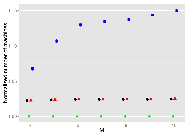
(a) Bivalued scenario

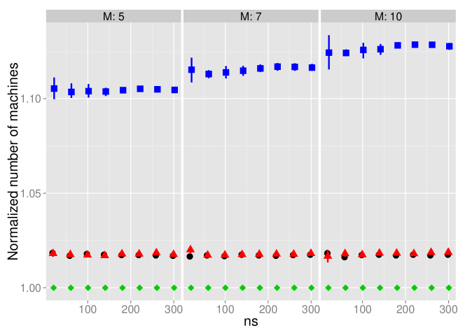
(b) Uniform scenario

Figure 2: Number of required machines

5.3.1 Execution time

We represent in Figure 3 the execution time of all heuristics, in both scenarios. There appears a difference between colgen and colgen_pd. In the Uniform scenario with low memory capacity, the execution time of colgen is at the same time very high and very unstable (it may reach $20\,\mathit{min}$), while colgen_pd remains under $30\,s$. With higher memory capacity, the execution time of colgen improves while colgen_pd gets slower; they become similar when 10 services are allowed on the same machine.

On the other hand, in the Bivalued case, the execution time of both variants increase when the memory capacity increases, and colgen_pd is always better than colgen.

Finally in all cases no_sharing confirms that it is a very cheap heuristic, and its execution time never exceeds $0.05\,s$.

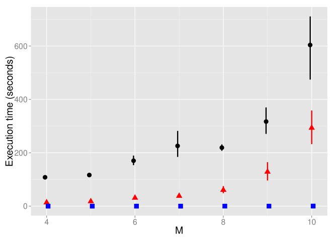
(a) Bivalued scenario

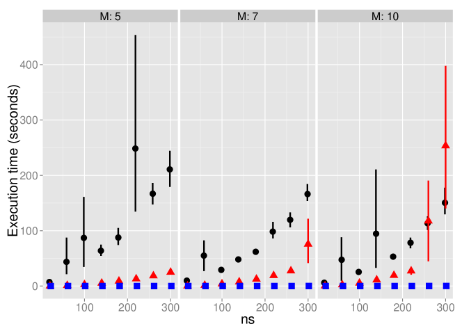
(b) Uniform scenario

Figure 3: Execution time

5.4 Reliability

We represent in Figure 4 the compliance of the services with their reliability constraint. This constraint is met if the point is below the black straight line. Because of the rounding step, the column generation heuristics fulfill easily the reliability bounds in average. Moreover, we observed (results are not displayed here due to lack of space) that the worse cases are very close to the line but remain below it, which is intended by construction of the heuristics.

In the Bivalued scenario, the column generation heuristics produce allocations that are even more reliable than in the Uniform scenario. This come from the fact that the big services are assigned to a large number of different configurations, and hence gain even more CPU after the rounding step.

There is a clear double advantage to the column generation-based algorithm, and especially colgen_pd, against no_sharing: it leads to more reliable allocations with a noticeably smaller number of machines.

(a) Bivalued scenario

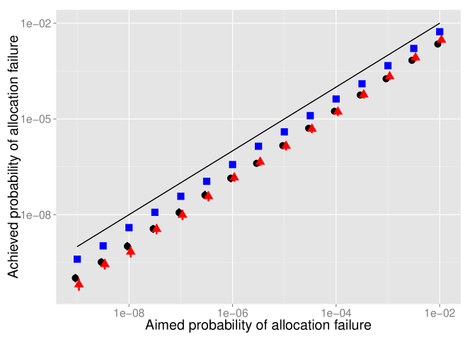
(b) Uniform scenario

Figure 4: Reliability constraints

5.5 Probability estimation algorithm

In Figure 5 we plot the execution time of the probability estimation algorithm of the reliability of a service as a function of the actual failure probability of the allocation. Obviously, when the failure probability decreases, the execution time increases, since the event that we try to capture is rarer. This estimate algorithm is efficient, since it can estimate an event of probability $10^{-17}$ in about $40\,s$. In our particular case, it is possible to further lower this execution time if we focus only on checking whether the failure probability requirement is not exceeded. Indeed, the requirements are lower than $10^{-9}$. By stopping the algorithm early, it is possible to determine whether the allocation is valid in at most $15\,s$.

We can remark that the estimate of failure probabilities in a solution returned by no_sharing is not expensive, since each service is allocated to exactly one configuration. Hence, at each step of the algorithm, we have only one draw for one binomial distribution, which is not the case with solutions that are provided by the other heuristics.

Figure 5: Execution Time of Probability Estimation Algorithm

6 Conclusion

The evolution of large computing platforms makes fault-tolerance issues crucial. With this respect, this paper considers a simple setting, with a set of services handling requests on an homogeneous cloud platform. To deal with fault tolerance issues, we assume that each service comes with a global demand and a reliability constraint. Our contribution follows two directions. First, with borrow and adapt from Applied Probability literature sophisticated techniques for estimating the failure probability of an allocation, that remains efficient even if the considered probability is very low ($10^{-10}$ for instance). Second, we borrow and adapt from the Mathematical Programming and Operations Research literature the use of Column Generation techniques, that enable to solve efficiently some classes of linear programs. The use of both techniques enables to solve in an efficient manner the resource allocation problem that we consider, under a realistic settings (both in terms of size of the problem and characteristics of the applications, for instance discrete unsplittable memory constraints) and we believe that it can be extended to many other fault-tolerant allocation problems.

References

- [1] W. Shih, S. Tseng, and C. Yang, “Performance study of parallel programming on cloud computing environments using mapreduce,” in International Conference on Information Science and Applications (ICISA). IEEE, 2010, pp. 1–8.
- [2] J. Dean and S. Ghemawat, “Mapreduce: Simplified data processing on large clusters,” Communications of the ACM, vol. 51, no. 1, pp. 107–113, 2008.
- [3] M. Zaharia, A. Konwinski, A. Joseph, R. Katz, and I. Stoica, “Improving mapreduce performance in heterogeneous environments,” in Proceedings of the 8th USENIX conference on Operating systems design and implementation. USENIX Association, 2008, pp. 29–42.
- [4] M. Bougeret, H. Casanova, M. Rabie, Y. Robert, and F. Vivien, “Checkpointing strategies for parallel jobs,” in High Performance Computing, Networking, Storage and Analysis (SC), 2011 International Conference for. IEEE, 2011, pp. 1–11.
- [5] F. Cappello, H. Casanova, and Y. Robert, “Checkpointing vs. migration for post-petascale supercomputers,” ICPP’2010, 2010.
- [6] A. Bouteiller, F. Cappello, J. Dongarra, A. Guermouche, T. Hérault, and Y. Robert, “Multi-criteria checkpointing strategies: response-time versus resource utilization,” in Euro-Par 2013 Parallel Processing. Springer, 2013, pp. 420–431.
- [7] C. Wang, Z. Zhang, X. Ma, S. S. Vazhkudai, and F. Mueller, “Improving the availability of supercomputer job input data using temporal replication,” Computer Science-Research and Development, vol. 23, no. 3-4, pp. 149–157, 2009.
- [8] K. Ferreira, J. Stearley, J. Laros III, R. Oldfield, K. Pedretti, R. Brightwell, R. Riesen, P. Bridges, and D. Arnold, “Evaluating the viability of process replication reliability for exascale systems,” in Proceedings of 2011 International Conference for High Performance Computing, Networking, Storage and Analysis. ACM, 2011, p. 44.
- [9] Q. Zhang, L. Cheng, and R. Boutaba, “Cloud computing: state-of-the-art and research challenges,” Journal of Internet Services and Applications, vol. 1, no. 1, pp. 7–18, 2010.
- [10] M. Armbrust, A. Fox, R. Griffith, A. Joseph, R. Katz, A. Konwinski, G. Lee, D. Patterson, A. Rabkin, I. Stoica et al., “Above the clouds: A berkeley view of cloud computing,” EECS Department, University of California, Berkeley, Tech. Rep. UCB/EECS-2009-28, 2009.
- [11] W. Cirne and E. Frachtenberg, “Web-scale job scheduling,” in Job Scheduling Strategies for Parallel Processing. Springer, 2013, pp. 1–15.
- [12] “Amazon elastic compute cloud (amazon ec2),” http://aws.amazon.com/fr/ec2/.
- [13] H. Van, F. Tran, and J. Menaud, “SLA-aware virtual resource management for cloud infrastructures,” in IEEE Ninth International Conference on Computer and Information Technology. IEEE, 2009, pp. 357–362.
- [14] R. Calheiros, R. Buyya, and C. De Rose, “A heuristic for mapping virtual machines and links in emulation testbeds,” in ICPP. IEEE, 2009, pp. 518–525.
- [15] O. Beaumont, L. Eyraud-Dubois, H. Rejeb, and C. Thraves, “Heterogeneous Resource Allocation under Degree Constraints,” IEEE Transactions on Parallel and Distributed Systems, 2012.
- [16] A. Berl, E. Gelenbe, M. Di Girolamo, G. Giuliani, H. De Meer, M. Dang, and K. Pentikousis, “Energy-efficient cloud computing,” The Computer Journal, vol. 53, no. 7, p. 1045, 2010.
- [17] A. Beloglazov and R. Buyya, “Energy efficient allocation of virtual machines in cloud data centers,” in 2010 10th IEEE/ACM International Conference on Cluster, Cloud and Grid Computing. IEEE, 2010, pp. 577–578.
- [18] M. R. Garey and D. S. Johnson, Computers and Intractability, a Guide to the Theory of NP-Completeness. W. H. Freeman and Company, 1979.
- [19] L. Epstein and R. van Stee, “Online bin packing with resource augmentation.” Discrete Optimization, vol. 4, no. 3-4, pp. 322–333, 2007.
- [20] D. Hochbaum, Approximation Algorithms for NP-hard Problems. PWS Publishing Company, 1997.
- [21] C. Barnhart, E. L. Johnson, G. L. Nemhauser, M. W. Savelsbergh, and P. H. Vance, “Branch-and-price: Column generation for solving huge integer programs,” Operations research, vol. 46, no. 3, pp. 316–329, 1998.
- [22] J. Desrosiers and M. E. Lübbecke, A primer in column generation. Springer, 2005.
- [23] K. Ranganathan, A. Iamnitchi, and I. Foster, “Improving data availability through dynamic model-driven replication in large peer-to-peer communities,” in Cluster Computing and the Grid, 2002. IEEE/ACM International Symposium on, 2002.
- [24] D. da Silva, W. Cirne, and F. Brasileiro, “Trading cycles for information: Using replication to schedule bag-of-tasks applications on computational grids,” in Euro-Par 2003 Parallel Processing, ser. Lecture Notes in Computer Science, H. Kosch, L. Böszörményi, and H. Hellwagner, Eds. Springer Berlin / Heidelberg, 2003, vol. 2790, pp. 169–180.
- [25] M. Lei, S. V. Vrbsky, and X. Hong, “An on-line replication strategy to increase availability in data grids,” Future Generation Computer Systems, vol. 24, no. 2, pp. 85 – 98, 2008. [Online]. Available: http://www.sciencedirect.com/science/article/pii/S0167739X07000830
- [26] H.-I. Hsiao and D. J. Dewitt, “A performance study of three high availability data replication strategies,” Distributed and Parallel Databases, vol. 1, pp. 53–79, 1993, 10.1007/BF01277520. [Online]. Available: http://dx.doi.org/10.1007/BF01277520
- [27] E. Santos-Neto, W. Cirne, F. Brasileiro, and A. Lima, “Exploiting replication and data reuse to efficiently schedule data-intensive applications on grids,” in Job Scheduling Strategies for Parallel Processing, ser. Lecture Notes in Computer Science, D. Feitelson, L. Rudolph, and U. Schwiegelshohn, Eds. Springer Berlin / Heidelberg, 2005, vol. 3277, pp. 54–103.
- [28] J. Dongarra, P. Beckman, P. Aerts, F. Cappello, T. Lippert, S. Matsuoka, P. Messina, T. Moore, R. Stevens, A. Trefethen et al., “The international exascale software project: a call to cooperative action by the global high-performance community,” International Journal of High Performance Computing Applications, vol. 23, no. 4, pp. 309–322, 2009.
- [29] “Eesi, ”the european exascale software initiative”, 2011,” http://www.eesi-project.eu/pages/menu/homepage.php.
- [30] F. Cappello, “Fault tolerance in petascale/exascale systems: Current knowledge, challenges and research opportunities,” International Journal of High Performance Computing Applications, vol. 23, no. 3, pp. 212–226, 2009.
- [31] O. Beaumont, L. Eyraud-Dubois, and H. Larchevêque, “Reliable service allocation in clouds,” in IPDPS’13 IEEE International Parallel & Distributed Processing Symposium, 2013.
- [32] L. Valiant, “The complexity of enumeration and reliability problems,” SIAM J. Comput., vol. 8, no. 3, pp. 410–421, 1979.
- [33] J. Provan and M. Ball, “The complexity of counting cuts and of computing the probability that a graph is connected,” SIAM Journal on Computing, vol. 12, p. 777, 1983.
- [34] H. Bodlaender and T. Wolle, “A note on the complexity of network reliability problems,” UU-CS, no. 2004-001, 2004.
- [35] Z. I. Botev and D. P. Kroese, “An efficient algorithm for rare-event probability estimation, combinatorial optimization, and counting,” Methodology and Computing in Applied Probability, vol. 10, no. 4, pp. 471–505, 2008.
- [36] O. Beaumont, P. Duchon, and P. Renaud-Goud, “Approximation algorithms for energy minimization in cloud service allocation under reliability constraints,” in HIPC’2013, IEEE international conference on High Performance Computing, Bangalore, 2013.
- [37] H. Chernoff, “A measure of asymptotic efficiency for tests of a hypothesis based on the sum of observations,” The Annals of Mathematical Statistics, vol. 23, no. 4, pp. 493–507, 1952.
- [38] W. Hoeffding, “Probability inequalities for sums of bounded random variables,” Journal of the American Statistical Association, vol. 58, no. 301, pp. 13–30, 1963.
- [39] O. Beaumont, L. Eyraud-Dubois, P. Pesneau, and P. Renaud-Goud, “Reliable service allocation in clouds with memory and capacity constraints,” in Resilience – EuroPar workshop, 2013.
- [40] “Gsl library,” http://www.gnu.org/software/gsl.
- [41] “Source code of the simulations,” http://graal.ens-lyon.fr/ prenaud/colgen/.