Strong Planck constraints on braneworld and non-commutative inflation

Abstract

We place observational likelihood constraints on braneworld and non-commutative inflation for a number of inflaton potentials, using Planck, WMAP polarization and BAO data. Both braneworld and non-commutative scenarios of the kind considered here are limited by the most recent data even more severely than standard general-relativity models. At more than 95 % confidence level, the monomial potential $V(\phi)\propto\phi^{p}$ is ruled out for $p\geq 2$ in the Randall–Sundrum (RS) braneworld cosmology and, for $p>0$, also in the high-curvature limit of the Gauss–Bonnet (GB) braneworld and in the infrared limit of non-commutative inflation, due to a large scalar spectral index. Some parameter values for natural inflation, small-varying inflaton models and Starobinsky inflation are allowed in all scenarios, although some tuning is required for natural inflation in a non-commutative spacetime.

1 Introduction

Experimental cosmology is living its golden age. Observations of the Cosmic Microwave Background (CMB) have been approaching the ideal precision, starting with WMAP [1, 2] and following with the first achievements of the Planck satellite [3]. This permitted to constrain a variety of inflationary scenarios in an unprecedented way [4, 5, 6, 7, 8, 9, 10, 11, 12] and to partly remove the huge model degeneracy surrounding the history of the early universe. An increasing number of theoretical proposals has been advanced to describe new physics beyond both the Standard Model and general relativity (GR), and it is becoming more and more important to appeal to experiments in order to focus one’s attention to the most promising candidates.

The purpose of this paper is to take advantage of modern data and revisit some high-energy models which thrived in the late 1990s and early 2000s: the braneworld (consult [13] for a review) and Brandenberger–Ho non-commutative inflation [14]. The first (section 2) is a class of string-inspired models where the observer lives in a four-dimensional manifold (the brane) embedded in five non-compact dimensions. The gravitational dynamics induced on the brane is modified with respect to standard cosmology, which leads to deviations from the inflationary predictions of general relativity. We will focus on two specific braneworld models, Randall–Sundrum (RS, [15, 16]) and Gauss–Bonnet (GB, [17, 18]). The non-commutative scenario of [14] and its developments [19, 20, 21, 22, 23, 24, 25, 26, 27, 28] (section 3) assume, in accordance with some quantum-gravity approaches, that spacetime is not an ordinary manifold but possesses a non-commutative structure, determined by a fundamental length scale and an intrinsic uncertainty relation on space and time interval measurements.

By now, it is clear that standard inflation with large-field potentials is under observational pressure, while small-varying inflaton models and potentials motivated by string theory or higher-curvature actions are favored [4, 10]. In all these cases, the dynamical cosmological equations are the same of general relativity, the only difference being in the choice of the potentials. The question is whether braneworld and non-commutative scenarios, where the dynamics is modified, fare better when the same types of potentials are considered. Performing a likelihood analysis of cosmological data (section 4), we shall see in sections 5 and 6 that this is not the case. Large-field potentials are even less viable than in standard cosmology, while small-varying inflaton models and Starobinsky inflation still survive but in a narrower parameter space. Overall, braneworld and non-commutative inflation do not present any advantage or characteristic signature with respect to standard cosmology, and in large portions of their parameter space they are actually excluded.

This drastic conclusion was not possible ten years ago, when constraints with the WMAP1 data [1] were imposed following the same method [29]. The area in the $(n_{\rm s},r)$ plane enclosed in likelihood contours was large enough to include most of the theoretical points of these scenarios, apart from the exponential potential in some cases. The resulting non-committal conclusion was that braneworld and non-commutative models could be discriminated from standard inflation by further data and near-future experiments. The shrinking of the likelihood areas has now come to the exciting point where we are in that ‘near future’ and we can finally place the desired constraints.

2 Braneworld inflation

In braneworld scenarios, the universe and its observers live in a (3+1)-dimensional manifold (a brane) embedded in a larger non-compact spacetime (the bulk). Such configuration, with a five-dimensional bulk, arises as the low-energy limit of the Calabi–Yau compactification of six dimensions in M theory [30, 31]. Assuming a Friedmann–Lemaître–Robertson–Walker (FLRW) background on the brane and that all the matter is confined therein (the 5D energy-momentum tensor is $T^{\mu\nu}\propto\delta(y_{b})\,{\rm diag}(\rho,-p,-p,-p,0)$, where $y_{b}$ is the brane position along the extra direction $y$), if the 5D gravitational action is the Einstein–Hilbert one (Randall–Sundrum model) one can show that the Friedmann equation acquires a quadratic correction [32, 33, 34],

$$H^{2}=\frac{\kappa_{4}^{2}}{6\lambda}\rho(2\lambda+\rho)+\frac{\cal E}{a^{4}}\,,$$ (2.1)

where $H=\dot{a}/a$ is the Hubble parameter, $a$ is the scale factor, a dot represents a derivative with respect to synchronous time $t$, $\kappa_{4}^{2}:=8\pi/m_{\rm Pl}^{2}$ includes the four-dimensional Planck mass $m_{\rm Pl}\approx 10^{19}\,\text{GeV}$, $\lambda$ is the brane tension and ${\cal E}=$const. is a dark radiation term. The RS model can be viewed as an intermediate scenario between the standard 4D (low-energy) evolution, $H^{2}\propto\rho$ and a braneworld scenario where higher-order curvature corrections, arising in the heterotic string [35], are included in the 5D action:

$$S=\frac{1}{2\kappa_{5}^{2}}\int d^{5}x\sqrt{-g_{5}}\left[R-2\Lambda_{5}+\alpha_{\rm GB}\left(R^{2}-4R_{\mu\nu}R^{\mu\nu}+R_{\mu\nu\rho\sigma}R^{\mu\nu\rho\sigma}\right)\right]+S_{\text{\tiny matter}}\,.$$ (2.2)

Here, $\kappa_{5}$ is the 5D gravitational coupling, $g_{5}$ is the determinant of the 5D metric, $R$ is the 5D Ricci scalar, $\Lambda_{5}<0$ is the bulk cosmological constant and $\alpha_{\rm GB}=1/(8g_{\rm s}^{2})>0$ is the coupling of the Gauss–Bonnet term, where $g_{\rm s}$ is the string energy scale. We omitted a boundary term in the action. The effective Friedmann equation on the brane is [36, 37, 38, 39]

$$H^{2}=\frac{c_{+}+c_{-}-2}{8\alpha_{\rm GB}}\,,$$ (2.3)

where $H$ is the Hubble parameter and, defining $\delta_{0}^{-1}:=\sqrt{\alpha_{\rm GB}/2}\,\kappa_{5}^{2}$,

$$c_{\pm}=\left[\sqrt{\left(1+4\alpha_{\rm GB}\Lambda_{5}/3\right)^{3/2}+\left(\delta/\delta_{0}\right)^{2}}\pm\delta/\delta_{0}\right]^{2/3},$$ (2.4)

$\delta=\rho+\lambda$ being the matter energy density decomposed into a matter contribution plus the brane tension $\lambda$. Expanding Eq. (2.3) to quadratic order in $\delta$, one recovers the Friedmann equation (2.1) of the RS scenario with vanishing 4D cosmological constant, provided some relations between the couplings of the model are satisfied. Therefore, one can now recognize three energy regimes:

$$H^{2}\approx\left(\frac{\kappa_{5}^{2}}{16\alpha_{\rm GB}}\right)^{2/3}\rho^{2/3}\quad{\rm when}\quad\delta/\delta_{0}\gg 1~{}~{}({\rm GB~{}regime}),$$ (2.5)

$$H^{2}\approx\frac{\kappa_{4}^{2}}{6\lambda}\rho^{2}\qquad\qquad~{}~{}{\rm when}\quad\lambda/\delta_{0}\ll\delta/\delta_{0}\ll 1~{}~{}({\rm RS~{}regime}),$$ (2.6)

$$H^{2}\approx\frac{\kappa_{4}^{2}}{3}\rho\qquad\qquad\qquad~{}{\rm when}\quad\rho/\delta_{0}\ll\delta/\delta_{0}\ll 1~{}~{}({\rm GR~{}regime}).$$ (2.7)

An economic way to treat all these regimes analytically is the patch formalism [28, 40], where one assumes the effective Friedmann equation

$$H^{2}=\beta_{q}^{2}\rho^{q}\,,$$ (2.8)

and $\beta_{q}$ and $q$ are constants. In different energy regimes and time intervals (the patches), $q$ acquires different values:

$$q=\begin{cases}1&({\rm GR}),\\ 2&({\rm RS})\,,\\ 2/3&({\rm GB})\,.\end{cases}$$ (2.9)

We focus on the case in which a minimally coupled scalar field $\phi$ is confined on the 3-brane. On the homogeneous and isotropic background, the energy density of $\phi$ is given by

$$\rho=\frac{1}{2}\dot{\phi}^{2}+V(\phi)\,,$$ (2.10)

where $V(\phi)$ is the potential of $\phi$. The inflaton satisfies the following equation of motion:

$$\ddot{\phi}+3H\dot{\phi}+V_{,\phi}(\phi)=0\,,$$ (2.11)

where $V_{,\phi}=dV/d\phi$.

The slow-roll (SR) parameters associated with the inflaton $\phi$ are

$$\epsilon_{\phi}:=-\frac{\dot{H}}{H^{2}}\,,\qquad\eta_{\phi}:=-\frac{\ddot{\phi}}{H\dot{\phi}}\,,\qquad\xi_{\phi}^{2}:=\frac{1}{H^{2}}\left(\frac{\ddot{\phi}}{\dot{\phi}}\right)^{\cdot}\,.$$ (2.12)

We also introduce the horizon-flow (HF) parameters [41, 42]

$$\epsilon_{0}:=\frac{H_{\rm inf}}{H}\,,\qquad\epsilon_{j+1}:=\frac{d\ln|\epsilon_{j}|}{dN}\,,\qquad j\geq 0\,,$$ (2.13)

where $H_{\rm inf}$ is the Hubble rate at some chosen time and $N:=\ln(a/a_{\rm i})$ is the number of e-folds; here $a_{i}=a(t_{\rm i})$ and $t_{\rm i}$ is the time at the onset of inflation. The evolution equation for the HF parameters is given by $\dot{\epsilon}_{j}=H\epsilon_{j}\epsilon_{j+1}$. The HF parameters are related to the first SR parameters by

$$\epsilon_{1} = \epsilon_{\phi}\,,$$ (2.14a)

$$\epsilon_{2} = 2\epsilon_{\phi}/q-2\eta_{\phi}\,,$$ (2.14b)

$$\epsilon_{2}\epsilon_{3} = 4\epsilon_{\phi}^{2}/q^{2}-2(1+2/q)\epsilon_{\phi}\eta_{\phi}+2\xi_{\phi}^{2}\,.$$ (2.14c)

The amplitudes of scalar and tensor perturbations are given, respectively, by [43, 44, 45, 46, 47, 48, 40]

$${\cal P}_{\rm s} = \frac{3q\beta_{q}^{2/q}}{25\pi^{2}}\frac{H^{4-2/q}}{2\epsilon_{1}}\,,$$ (2.15)

$${\cal P}_{\rm t} = \frac{48q\beta_{q}^{2/q}}{25\pi^{2}}\frac{H^{4-2/q}}{2\zeta_{q}}\,,$$ (2.16)

where

$$\zeta_{q}=\begin{cases}1&({\rm GR}),\\ 2/3&({\rm RS})\,,\\ 1&({\rm GB})\,.\end{cases}$$ (2.17)

The spectra (2.15) and (2.16) should be evaluated when the modes with the physical wave number $k/a$ crossed the Hubble radius during inflation ($k/a=H$). The spectral indices of scalar and tensor perturbations evaluated at the Hubble radius crossing are

$$n_{\rm s}-1 = \frac{d\ln{\cal P}_{\rm s}}{d\ln k}=-(4-2/q)\epsilon_{1}-\epsilon_{2}\,,$$ (2.18)

$$n_{\rm t} = \frac{d\ln{\cal P}_{\rm t}}{d\ln k}=-(4-2/q)\epsilon_{1}\,.$$ (2.19)

The tensor-to-scalar ratio is

$$r=\frac{{\cal P}_{\rm t}}{{\cal P}_{\rm s}}=\frac{16\epsilon_{1}}{\zeta_{q}}=-\frac{8q}{(2q-1)\zeta_{q}}n_{\rm t}\,,$$ (2.20)

where we used Eq. (2.19). The consistency relation is given by

$$r = -8n_{\rm t}\qquad~{}\,({\rm GR~{}and~{}RS})\,,$$ (2.21)

$$r = -16n_{\rm t}\qquad({\rm GB})\,.$$ (2.22)

The runnings of the spectral indices, $\alpha_{{\rm s},{\rm t}}=dn_{{\rm s},{\rm t}}/d\ln k$, read

$$\alpha_{\rm s} = -(4-2/q)\epsilon_{1}\epsilon_{2}-\epsilon_{2}\epsilon_{3}\,,$$ (2.23)

$$\alpha_{\rm t} = -(4-2/q)\epsilon_{1}\epsilon_{2}\,,$$ (2.24)

which are second order in the slow-roll parameters.

3 Non-commutative inflation

In this section, we briefly recall the main features of non-commutative inflation [14, 27, 28]. Time and space measurements are subject to an uncertainty relation $\Delta t\Delta x_{p}\geq l_{\rm s}^{2}$, where $l_{\rm s}\equiv M_{\rm s}^{-1}$ is a fundamental length scale (possibly identifiable with the string length [49, 50, 51]) and $x_{p}$ is the physical spatial coordinate. Due to this intrinsic scale in the geometry, coordinates do not commute; an algebra preserving the maximal symmetry of the FLRW background is $[\tau,x]=il_{\rm s}^{2}$, where $\tau:=\int a\,dt$ and $x$ is a comoving spatial coordinate. In this setting, there appears a comoving scale $k_{0}(\delta)$ dependent on the parameter $\delta:=(M_{\rm s}/H)^{2}$. The space of comoving wave numbers is divided into two regions, one including small-scale perturbations generated in the ultraviolet (UV), i.e., inside the Hubble horizon ($H\ll M_{\rm s}$) and the other describing the infrared (IR), large-scale perturbations created outside the horizon ($H\gg M_{\rm s}$). Somewhat counterintuitively, the UV region corresponds to a weak non-commutative regime, while the IR region is characterized by strong non-commutative effects.

The spectra of scalar and tensor perturbations turn out to be

$${\cal P}(\delta,\,H,\,\phi)={\cal P}^{(c)}(H,\,\phi)\,\Sigma^{2}(\delta)\,,$$ (3.1)

where ${\cal P}^{(c)}={\cal P}(\Sigma\!\!=\!\!1)$ is the amplitude in the commutative limit and $\Sigma(\delta)$ is a function encoding non-commutative effects. The same factor $\Sigma$ multiplies both the tensor and scalar amplitudes, so their ratio is unchanged.

Let us concentrate on the IR limit, which bears the largest non-commutative effect. The spectra (3.1) are evaluated at the moment when the perturbation with comoving wave-number $k$ is generated. To lowest order in the HF parameters,

$$\frac{d\ln\Sigma^{2}}{d\ln k}=\sigma\epsilon_{1}\,,$$ (3.2)

where $\sigma=\sigma(\delta)$ is a function of $\delta$ such that $\dot{\sigma}=O(\epsilon_{1})$. The commutative spacetime corresponds to $\sigma=0$.

Let us accommodate the effect of non-commutativity for $q=1$ in Eq. (2.8). Then, the spectral indices (2.18) and (2.19) are modified to

$$n_{\rm s}-1 = -(2-\sigma)\epsilon_{1}-\epsilon_{2}\,,$$ (3.3)

$$n_{\rm t} = -(2-\sigma)\epsilon_{1}\,.$$ (3.4)

The tensor-to-scalar ratio reads

$$r=16\epsilon_{1}=-\frac{16}{2-\sigma}n_{\rm t}\qquad(\sigma\neq 2)\,.$$ (3.5)

Consequently, the runnings of the spectral indices are

$$\alpha_{\rm s} = -(2-\sigma)\epsilon_{1}\epsilon_{2}-\sigma\bar{\sigma}\epsilon_{1}^{2}-\epsilon_{2}\epsilon_{3}\,,$$ (3.6)

$$\alpha_{\rm t} = -(2-\sigma)\epsilon_{1}\epsilon_{2}-\sigma\bar{\sigma}\epsilon_{1}^{2}\,,$$ (3.7)

where $\bar{\sigma}:=-\dot{\sigma}/(H\sigma\epsilon_{1})$.

In the infrared region, two classes of non-commutative models have been proposed [14]. In the first one (class 1), the FLRW 2-sphere is factored out in the measure $z_{k}$ of the effective perturbation action. The measure is thus given by the product of the commutative contribution $z$ times a $(1+1)$-dimensional correction factor. In the class-2 choice, the scale factor in the measure is everywhere substituted by an effective scale $a_{\text{\tiny eff}}$ whose time dependence is smeared out by non-local effects; since $z\propto a$, then $z_{k}=za_{\text{\tiny eff}}/a$. Inequivalent prescriptions on the ordering of the *-product in the perturbation action further split these two classes, but in the IR limit they give almost the same predictions [27]. In this limit, the parameter $\sigma$ approaches the constant value $\sigma=6$ in class-1 models and $\sigma=2$ in class-2 models [27].

From Eqs. (3.3)-(3.5), it follows that

$$n_{\rm s}-1=4\epsilon_{1}-\epsilon_{2}\,,\quad\,n_{\rm t}=r/4\qquad(\sigma=6),$$ (3.8)

$$n_{\rm s}-1=-\epsilon_{2}\,,\qquad\quad n_{\rm t}=0\quad\qquad(\sigma=2).$$ (3.9)

The standard GR commutative consistency relation $n_{\rm t}=-r/8$ is thus deformed by non-commutativity.

4 Likelihood analysis

In order to place observational constraints on the inflationary models discussed in Secs. 2 and 3, the power spectra ${\cal P}_{\rm s}$ and ${\cal P}_{\rm t}$ are expanded around the pivot wave number $k_{0}$, as

$$\ln{\cal P}_{\rm s}(k) = \ln{\cal P}_{\rm s}(k_{0})+[n_{\rm s}(k_{0})-1]x+\frac{\alpha_{\rm s}(k_{0})}{2}x^{2}+O(x^{3}),$$ (4.1a)

$$\ln{\cal P}_{\rm t}(k) = \ln{\cal P}_{\rm t}(k_{0})+n_{\rm t}(k_{0})x+\frac{\alpha_{\rm t}(k_{0})}{2}x^{2}+O(x^{3}),$$ (4.1b)

where $x=\ln(k/k_{0})$. For the scales relevant to the observed CMB anisotropies (the multipoles $2\leq\ell\lesssim 2500$), $x$ is smaller than 7. Since $\alpha_{{\rm s},{\rm t}}(k_{0})$ are of the order of $\epsilon_{j}^{2}$, the third and fourth terms on the right-hand side of Eq. (4.1) are suppressed relatively to the first two terms. In the slow-roll expressions for $n_{\rm s,t}$ and $r$, we neglect the second-order terms, which are always subdominant with respect to the $O(\epsilon_{j})$ parts. On the other hand, we retain the terms $\alpha_{\rm s,t}x^{2}=O(\epsilon_{j}^{2}\,x^{2})$ because, although the runnings are second order in slow-roll parameters, they give rise to non-negligible effects for large $x$. This mixed truncation scheme is fairly standard in CMB analysis.

We choose the pivot wavenumber to be

$$k_{0}=0.05~{}{\rm Mpc}^{-1}\,.$$ (4.2)

This is different from the value $k_{0}=0.002~{}{\rm Mpc}^{-1}$ used by the Planck team [3], but we confirm that the likelihood results are insensitive to the choice of $k_{0}$ for the scales relevant to the observed CMB anisotropies.

We run the CosmoMC code [52, 53] by using the recent data of Planck [3], WMAP polarization (WP) [2], Baryon Acoustic Oscillations (BAO) [54] and high-$\ell$ ACT/SPT temperature data [55]. We use the big-bang nucleosynthesis consistency relation, by which the helium fraction $Y_{p}$ is expressed in terms of $N_{\rm eff}$ and the baryon fraction $\Omega_{b}h^{2}$. The flat $\Lambda$CDM model is assumed with $N_{\rm eff}=3.046$ relativistic degrees of freedom and with instant reionization.

We have six inflationary observables ${\cal P}_{\rm s}(k_{0})$, $n_{\rm s}(k_{0})$, $n_{\rm t}(k_{0})$, $r(k_{0})={\cal P}_{\rm t}(k_{0})/{\cal P}_{\rm s}(k_{0})$, $\alpha_{\rm s}(k_{0})$, and $\alpha_{\rm t}(k_{0})$ to confront with the data. In the slow-roll framework, these reduce to four observables for given values of $q$ and $\sigma$. In both braneworld and non-commutative inflation the scalar spectral index and the tensor-to-scalar ratio can be expressed as $n_{\rm s}-1=-(4-2/q-\sigma)\epsilon_{1}-\epsilon_{2}$ and $r=16\epsilon_{1}/\zeta_{q}$, so that $\epsilon_{1}$ and $\epsilon_{2}$ are inverted to give

$$\epsilon_{1} = \frac{\zeta_{q}}{16}r\,,$$ (4.3)

$$\epsilon_{2} = -\frac{\zeta_{q}}{16}(4-2/q-\sigma)r+1-n_{\rm s}\,,$$ (4.4)

where we omitted the $k_{0}$ dependence. Substituting these relations into Eqs. (3.4) and (3.7), $n_{\rm t}$ and $\alpha_{\rm t}$ are known. The scalar running includes the additional parameter $\epsilon_{3}$, so we need to vary the four parameters ${\cal P}_{\rm s}$, $n_{\rm s}$, $r$ and $\epsilon_{3}$ in the likelihood analysis. The slow-roll parameter $\epsilon_{3}$ is smaller than $O(0.01)$. We have run the numerical code by setting the prior $\epsilon_{3}<0.05$ and found that the likelihood results are practically the same as those obtained for $\epsilon_{3}=0$. Therefore, we set $\epsilon_{3}=0$ in the whole likelihood analysis that follows. By assuming $\epsilon_{3}=0$, we reduce the free parameters to only three: ${\cal P}_{\rm s}$, $n_{\rm s}$ and $r$. The other variables $\alpha_{\rm s}$, $n_{\rm t}$ and $\alpha_{\rm t}$ are functions of these free parameters, so they are non-vanishing. We also tried the case where the runnings $\alpha_{\rm s}$ and $\alpha_{\rm t}$ are set to 0 and found that the results are practically identical to those derived for $\epsilon_{3}=0$.

The consistency relations are different depending on the scenarios we study, see Eqs. (2.21), (2.22), (3.8) and (3.9). We run the CosmoMC code for these four cases separately. As we will see, the likelihood results are insensitive to the change of the consistency relations. The scalar power spectrum is constrained to be ${\cal P}_{\rm s}(k_{0})\approx 2.2\times 10^{-9}$ for the pivot wave number (4.2). This information can be used to place bounds on some parameters of the theories.

We note that, in the context of slow-roll single-field inflation, the non-linear parameter $f_{\rm NL}^{\rm local}$ describing the scalar non-Gaussianities in the squeezed limit is of the order of the slow-roll parameters [56, 57, 58]. This is consistent with the recent Planck constraint $f_{\rm NL}^{\rm local}=2.7\pm 5.8$ (68 % confidence-level, CL) [59]. Since we focus on the slow-roll single-field framework, the local non-Gaussianities do not provide additional bounds on the models studied in this paper [60].

References [45, 46, 48, 29] followed the same method but applied to one of the first datasets of precision cosmology, the first-year release of WMAP [1]. In Refs. [45, 46], it was shown that, in the RS braneworld, the quadratic potential $V\propto\phi^{2}$ was inside the 95 % CL boundary but outside the 68 % CL contour. In the GB braneworld, the quadratic potential entered the 68 % CL region constrained by WMAP1 data [48]. The same happened for the quartic potential $V\propto\phi^{4}$, but in the GB limit ($\delta/\delta_{0}\gg 1$) the model was outside the 95 % CL boundary. In Ref. [29], two of the present authors studied observational constraints on hybrid scenarios of non-commutative braneworlds. The effect of non-commutativity allowed the possibility, with WMAP1 data, to rescue models disfavored in standard GR.

Later studies on braneworld and non-commutative inflation exploited more recent data but without extracting the likelihood bounds from new numerical simulations. The RS braneworld was compared against WMAP3 [61, 62] and WMAP5 data [63]: the potentials with small-field variations turned out to be favored [62] and the quartic potential excluded [61]. The quartic potential was also excluded in the GB braneworld by WMAP3 data [61]. Planck data were recently used also in [64], but on a DGP brane model different from the present ones. Reference [61] also studied non-commutative inflation in the IR limit, using the patch formalism of [40] and WMAP3 data, which led to the exclusion of quadratic and quartic potentials in the $\sigma=6$ model. These potentials have been ruled out also by Planck data, but only in the UV mild non-commutative regime [65]. All of these works based their conclusions (which agree with ours, whenever a comparison is possible) on the bounds on the scalar index, on its running and on the tensor-to-scalar ratio, sometimes reusing the likelihood contour plots of [29] or of the WMAP and Planck teams. In this respect, the present analysis constitutes the first significant update on braneworld and non-commutative scenarios in the post-WMAP era.

5 Observational constraints on braneworld inflation

We study observational constraints on several inflaton potentials in the context of RS ($q=2$) and GB ($q=2/3$) braneworlds in commutative spacetime ($\sigma=0$). Under the slow-roll approximation ($\dot{\phi}^{2}/2\ll V(\phi)$ and $|\ddot{\phi}|\ll|3H\dot{\phi}|$), Eqs. (2.8) and (2.11) read

$$H^{2}\approx\beta_{q}^{2}V^{q}\,,$$ (5.1)

$$3H\dot{\phi}+V_{,\phi}\approx 0\,.$$ (5.2)

Taking the time derivative of Eq. (5.1) and using Eq. (5.2), the slow-roll parameter $\epsilon_{\phi}=\epsilon_{1}=-\dot{H}/H^{2}$ reads

$$\epsilon_{\phi}=\frac{qV_{,\phi}^{2}}{6\beta_{q}^{2}V^{q+1}}\,.$$ (5.3)

Similarly, we also obtain the following relation:

$$\eta_{\phi}=-\epsilon_{\phi}+\frac{V_{,\phi\phi}}{3\beta_{q}^{2}V^{q}}\,.$$ (5.4)

The scalar power spectrum (2.15) can be expressed as

$${\cal P}_{\rm s}=\frac{9\beta_{q}^{6}V^{3q}}{25\pi^{2}V_{,\phi}^{2}}\,.$$ (5.5)

On using Eqs. (2.14a) and (2.14b), the scalar spectral index (2.18) and the tensor-to-scalar ratio (2.20) read

$$n_{\rm s} = 1-\frac{1}{3\beta_{q}^{2}V^{q}}\left(3q\frac{V_{,\phi}^{2}}{V}-2V_{,\phi\phi}\right)\,,$$ (5.6)

$$r = \frac{8q}{3\beta_{q}^{2}\zeta_{q}}\frac{V_{,\phi}^{2}}{V^{q+1}}\,.$$ (5.7)

Under the slow-roll approximation, the number of e-foldings from the end of inflation (field value $\phi_{\rm f}$) to the epoch with the field value $\phi$ is given by

$$N=3\beta_{q}^{2}\int_{\phi_{\rm f}}^{\phi}d\tilde{\phi}\,\frac{V^{q}}{V_{,\tilde{\phi}}}\,.$$ (5.8)

In the following, we show observational constraints on the models for $N=50$ and $60$. Note that the value of $N$ can be different depending on the cosmological history after inflation [66]. One possible effect on the value of $N$ comes from the reheating stage after inflation. If reheating is caused by a perturbative decay of $\phi$, the Universe is matter dominated for the inflaton potential approximated as $V(\phi)\simeq m^{2}(\phi-\phi_{0})^{2}/2$ around the minimum. In the framework of GR, the number of e-foldings is modified depending on the reheating temperature $T_{\rm reh}$, as

$$N\simeq 56-\frac{2}{3}\ln\frac{10^{16}\,{\rm GeV}}{\rho_{\rm end}^{1/4}}-\frac{1}{3}\ln\frac{10^{9}\,{\rm GeV}}{T_{\rm reh}}\,,$$ (5.9)

where $\rho_{\rm end}$ is the energy density of the Universe at the end of inflation.

In the RS braneworld scenario, the $\rho^{2}$ term in the background equation could dominate during reheating and one may expect a change in the value of $N$. If the $\rho^{2}$-dominated phase, where $H^{2}\propto a^{-6}$, ends before the completion of reheating, it gives rise to a change $\Delta N=(1/6)\ln(\rho_{\rm end}/\rho_{T})$ [67], where $\rho_{T}=2\lambda$ represents the energy density of the Universe at the transition from $\rho^{2}$ to $\rho$ dominating regime. Because of the coefficient $1/6$ and the logarithmic dependence of the ratio $\rho_{\rm end}/\rho_{T}$, the modification to $N$ cannot be so large. In non-commutative models, the background equation is not modified and reheating proceeds in a similar way as in GR. Therefore, in most cases $N$ ranges between 50 and 60. For completeness, below we will quote experimental bounds also for lower and higher values of $N$.

5.1 Monomial inflation

Let us first study monomial inflation [68] with the monomial potential

$$V(\phi)=V_{0}\phi^{p}\,,$$ (5.10)

where $V_{0}$ and $p$ are positive constants. The field value at the end of inflation is determined by the condition $\epsilon_{\phi}(\phi_{\rm f})=1$, i.e., $\phi_{\rm f}^{p(q-1)+2}=p^{2}qV_{0}^{1-q}/(6\beta_{q}^{2})$. Integrating Eq. (5.8), the field $\phi$ can be expressed in terms of $N$, as

$$\phi^{p(q-1)+2}=\frac{p}{6\beta_{q}^{2}V_{0}^{q-1}}\left[2(pq-p+2)N+pq\right]\,.$$ (5.11)

From Eqs. (5.6) and (5.7) we obtain

$$n_{\rm s} = 1-\frac{p(6q-4)+4}{2N(pq-p+2)+pq}\,,$$ (5.12)

$$r = \frac{16pq}{\zeta_{q}}\frac{1}{2N(pq-p+2)+pq}\,.$$ (5.13)

We discuss the RS and GB cases separately.

5.1.1 RS braneworld

In the RS case, the observables (5.12) and (5.13) reduce to

$$n_{\rm s} = 1-\frac{2(2p+1)}{N(p+2)+p}\,,$$ (5.14)

$$r = \frac{24p}{N(p+2)+p}\,.$$ (5.15)

When $N=60$, these are given by $n_{\rm s}=0.9669$, $r=0.1326$ for $p=1$, $n_{\rm s}=0.9587$, $r=0.1983$ for $p=2$, and $n_{\rm s}=0.9505$, $r=0.2637$ for $p=4$, respectively.

In Fig. 2, we plot the observational contours in the $(n_{\rm s},r)$ plane derived by the joint data analysis of Planck+WP+BAO+high-$\ell$. We also show the theoretical values (5.14) and (5.15) for $p=1,2,4$ with $N=50,60$. The potentials $V(\phi)=V_{0}\phi^{p}$ with $p\geq 2$ are outside the 95 % CL observational contour for both $N=50$ and 60. For $N>70$, the theoretical line goes outside the 95 % CL region. Although a small $N$ may be allowed by modifying the reheating scenario, for $p=1,2,4$ the model is outside the 95 % CL boundary when $N<52$.

The linear potential $V(\phi)=V_{0}\phi$ arises for a string axion in type IIB compactification in the presence of wrapped branes [69]. This case is marginally inside the 95 % CL boundary for $N=60$, but it is outside the 95 % CL region for $N=50$. These tensions come from the fact that the tensor-to-scalar ratio gets even larger than that in GR for the same value of $p$.

Note that the exponential potential $V(\phi)=V_{0}e^{-\alpha\phi/m_{\rm Pl}}$ [70] corresponds to the limit $p\to\infty$, i.e., $n_{\rm s}=1-4/(N+1)$ and $r=24/(N+1)$. In this case, the model is far outside the 95 % CL observational boundary.

5.1.2 GB braneworld

In the GB case,

$$n_{\rm s} = 1-\frac{6}{N(6-p)+p}\,,$$ (5.16)

$$r = \frac{16p}{N(6-p)+p}\,.$$ (5.17)

When $N=60$, we have $n_{\rm s}=0.9801$, $r=0.0532$ for $p=1$, $n_{\rm s}=0.9752$, $r=0.1322$ for $p=2$, and $n_{\rm s}=0.9516$, $r=0.5161$ for $p=4$, respectively.

As we see in Fig. 2, the potentials with $p>0$ are outside the 95 % CL boundary. Even for the linear potential ($p=1$) where $r$ is smaller than 0.1, the model is in tension with the data because of the tight upper bound on $n_{\rm s}$. The model is excluded for $N>48$ at the 95 % CL. Thus, monomial inflation is observationally disfavored in both the RS and the GB case.

5.2 Natural inflation

Natural inflation [71] is characterized by the potential

$$V(\phi)=V_{0}\left[1+\cos(\phi/f)\right]\,,$$ (5.18)

where $V_{0}$ and $f$ are positive constants. In particular, $f$ is the energy scale at which the global symmetry associated with this model is broken.

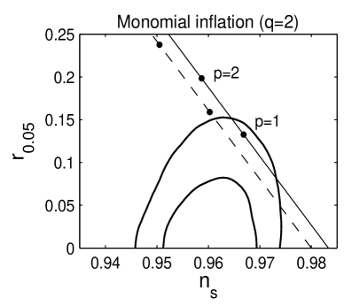
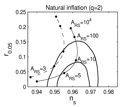
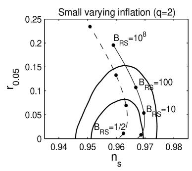
Figure 1: Two-dimensional observational constraints on the RS braneworld ($q=2$) in the ($n_{\rm s},r$) plane. Each panel corresponds to monomial inflation (top), natural inflation (middle), and small-varying inflaton models (bottom). The consistency relation $r=-8n_{\rm t}$ is assumed. The two contours show the 68 % (inside) and 95 % (outside) CL boundaries, respectively. The solid and dashed curves correspond to the theoretical predictions for $N=60$ and 50, respectively.

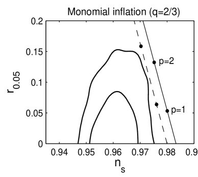
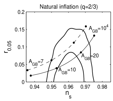
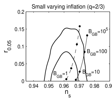
Figure 2: Two-dimensional observational constraints on the GB braneworld ($q=2/3$) in the ($n_{\rm s},r$) plane for monomial inflation (top), natural inflation (middle), and small-varying inflaton models (bottom). The consistency relation $r=-16n_{\rm t}$ is assumed. The meanings of observational contours and theoretical curves are the same as shown in Fig. 2.

5.2.1 RS braneworld

In the RS braneworld, the slow-roll parameter $\epsilon_{\phi}$ is given by

$$\epsilon_{\phi}=\frac{1}{3A_{\rm RS}}\frac{1-x}{(1+x)^{2}}\,,$$ (5.19)

where $A_{\rm RS}=\beta_{2}^{2}V_{0}f^{2}$ and $x:=\cos(\phi/f)$. Since we focus on the regime $0<\phi<\pi f$, the variable $x$ is in the range $-1<x<1$. The coefficient $\beta_{2}^{2}$ in Eq. (2.8) is related to the brane tension $\lambda$ and the 4-dimensional Planck mass $m_{\rm Pl}$, as $\beta_{2}^{2}=4\pi/(3m_{\rm Pl}^{2}\lambda)$ [34]. Then, the parameter $A_{\rm RS}$ can be expressed as

$$A_{\rm RS}=\frac{4\pi}{3}\frac{V_{0}}{\lambda}\left(\frac{f}{m_{\rm Pl}}\right)^{2}.$$ (5.20)

We are considering the high-energy regime in which the $\rho^{2}/\lambda$ term dominates over $\rho$, i.e., $V_{0}/\lambda\gg 1$. In order to realize a sufficient amount of inflation, we require that $A_{\rm RS}>O(1)$ (unless $\phi$ be initially extremely close to 0). In GR, the symmetry-breaking scale $f$ is constrained to be $f>0.9m_{\rm Pl}$ from the Planck data [10]. In the RS braneworld, it is possible to realize inflation even when $f$ is smaller than $m_{\rm Pl}$.

The end of inflation corresponds to $x_{\rm f}=-1+(\sqrt{24A_{\rm RS}+1}-1)/(6A_{\rm RS})$, where $x_{\rm f}=\cos(\phi_{\rm f}/f)$. The number of e-foldings is given by

$$N=6A_{\rm RS}\ln\frac{1-x_{\rm f}}{1-x}+3A_{\rm RS}(x_{\rm f}-x)\,.$$ (5.21)

From Eqs. (5.6) and (5.7), we have

$$n_{\rm s} = 1-\frac{2}{3A_{\rm RS}}\frac{3-2x}{(1+x)^{2}}\,,$$ (5.22)

$$r = \frac{8}{A_{\rm RS}}\frac{1-x}{(1+x)^{2}}\,.$$ (5.23)

For a given $A_{\rm RS}$, we can numerically obtain the values of $x$ at $N=50$ and 60 by using Eq. (5.21). Then, the scalar spectral index and the tensor-to-scalar ratio are evaluated from Eqs. (5.22) and (5.23).

In the limit that $A_{\rm RS}\gg 1$, we have $x_{\rm f}\to-1$ and $x\to 1+2W[-e^{-(N+6A_{\rm RS})/(6A_{\rm RS})}]$ from Eq. (5.21), where $W(z)$ is the Lambert $W$ function. Substituting this into Eqs. (5.22)-(5.23) and taking the limit $A_{\rm RS}\to\infty$, it follows that $n_{\rm s}\to 1-5/(2N)$ and $r\to 12/N$ ($n_{\rm s}=0.9583$ and $r=0.2$ for $N=60$). These correspond to the values (5.14) and (5.15) with $p=2$ and $N\gg 1$, so that the model approaches monomial inflation with the potential $V=V_{0}\phi^{2}$ for $A_{\rm RS}\to\infty$.

For decreasing $A_{\rm RS}$, the tensor-to-scalar ratio gets smaller. In the regime $A_{\rm RS}\gg 1$, the scalar spectral index gets larger as $A_{\rm RS}$ decreases, but it starts to decrease for $A_{\rm RS}\lesssim 10$. In Fig. 2, we plot the numerical values of $n_{\rm s}$ and $r$ as a function of $A_{\rm RS}$ in the range $3\leq A_{\rm RS}\leq 10^{4}$ for $N=50$ and 60. From the joint data analysis of Planck+WP+BAO+high-$\ell$, the parameter $A_{\rm RS}$ is constrained to be

$$3.5<A_{\rm RS}<49\quad(95\,\%\,{\rm CL})\quad{\rm for}~{}N=60,$$ (5.24)

$$5.0<A_{\rm RS}<11\quad(95\,\%\,{\rm CL})\quad{\rm for}~{}N=50.$$ (5.25)

The constraints on $A_{\rm RS}$ become weaker at larger $N$. For example, $3.1<A_{\rm RS}<75\,(95\,\%\,{\rm CL})$ for $N=80$. For small values of $N$, the model is excluded at 95$\%$ CL if $N<48$. The upper and lower bounds on $A_{\rm RS}$ come from the constraints on $r$ and $n_{\rm s}$, respectively. The bound (5.24) can be recast as $0.91<\sqrt{V_{0}/\lambda}\,(f/m_{\rm Pl})<3.4$, so a symmetry-breaking scale $f$ smaller than $m_{\rm Pl}$ can be allowed for $V_{0}/\lambda\gg 1$. We note that, only when $N>57$, there are some parameter values in which the model is inside the 68 % CL observational contour.

5.2.2 GB braneworld

In the GB braneworld, the slow-roll parameter reads

$$\epsilon_{\phi}=\frac{1}{9A_{\rm GB}}\frac{1-x}{(1+x)^{2/3}}\,,$$ (5.26)

where $A_{\rm GB}=\beta_{2/3}^{2}f^{2}V_{0}^{-1/3}$. The number of e-foldings is given by

$$N=3A_{\rm GB}\int_{x_{\rm f}}^{x}d\tilde{x}\,\frac{(1+\tilde{x})^{2/3}}{1-\tilde{x}^{2}}\,,$$ (5.27)

where $x_{\rm f}=\cos(\phi_{\rm f}/f)$ is known by the condition $\epsilon_{\phi}(x_{\rm f})=1$. Equation (5.27) can be analytically integrated, but we do not write its explicit expression because of its complexity.

The scalar spectral index and the tensor-to-scalar ratio are

$$n_{\rm s} = 1-\frac{2}{3A_{\rm GB}}\frac{1}{(1+x)^{2/3}}\,,$$ (5.28)

$$r = \frac{16}{9A_{\rm GB}}\frac{1-x}{(1+x)^{2/3}}\,.$$ (5.29)

For a given $A_{\rm GB}$, the values of $x$ corresponding to $N=50$ and 60 are known from Eq. (5.27), so that $n_{\rm s}$ and $r$ are evaluated from Eqs. (5.28) and (5.29).

In Fig. 2, we plot the theoretical values of $n_{\rm s}$ and $r$ in the range $7\leq A_{\rm GB}\leq 10^{4}$. When $A_{\rm GB}=7$ and $N=60$, we have that $n_{\rm s}=0.9377$ and $r=0.0181$, in which case the model is outside the 95 % CL boundary. For increasing $A_{\rm GB}$, both $n_{\rm s}$ and $r$ get larger, so that the model enters the 95 % CL region. In the limit that $A_{\rm GB}\to\infty$, $n_{\rm s}$ and $r$ approach the values (5.16) and (5.17) with $p=2$. In this limit, the model is again outside the 95 % CL contour. Then, the parameter $A_{\rm GB}$ is constrained to be

$$8.7<A_{\rm GB}<38\quad(95\,\%\,{\rm CL})\quad{\rm for}~{}N=60,$$ (5.30)

$$10<A_{\rm GB}<55\quad~{}(95\,\%\,{\rm CL})\quad{\rm for}~{}N=50.$$ (5.31)

For larger $N$, the constraints on $A_{\rm GB}$ become stronger. For example, we obtain $8.1<A_{\rm GB}<22\,(95\,\%\,{\rm CL})$ for $N=80$. With small values of $N$, the model is excluded at 95$\%$ CL if $N<42$. If $N>53$, then there is some non-trivial parameter space in which the model is inside the 68 % CL boundary.

5.3 Small varying inflaton models

In GR there are some inflationary models in which the variation of the field from the epoch at which the perturbations relevant to the CMB crossed the Hubble radius to the end of inflation is smaller than the order of the Planck mass $m_{\rm Pl}$. We call such models small-varying inflaton models. We call that the situation of this small variation can be subject to change in the RS and GB braneworld scenarios. For concreteness, we consider the following potential:

$$V(\phi)=V_{0}(1-e^{-\alpha\phi/m_{\rm Pl}})^{2}\,,$$ (5.32)

where $V_{0}$ and $\alpha$ are positive constants. In the Starobinsky model, where the Lagrangian is given by $f(R)=R+R^{2}/(6M^{2})$ [72], the potential in the Einstein frame corresponds to (5.32) with $V_{0}=3M^{2}m_{\rm Pl}^{2}/(32\pi)$ and $\alpha=4\sqrt{\pi/3}$ [73]. In the following, when we mention the Starobinsky model, it means the potential $V(\phi)=V_{0}(1-e^{-4\sqrt{\pi/3}\,\phi/m_{\rm Pl}})^{2}$ in the Einstein frame.

5.3.1 RS braneworld

In the RS case, the slow-roll parameter is given by

$$\epsilon_{\phi}=\frac{4}{3B_{\rm RS}}\frac{y^{2}}{(1-y)^{4}}\,,$$ (5.33)

where $B_{\rm RS}=\beta_{2}^{2}V_{0}m_{\rm Pl}^{2}/\alpha^{2}$ and $y=e^{-\alpha\phi/m_{\rm Pl}}$. The parameter $B_{\rm RS}$ can be expressed in terms of the brane tension $\lambda$, as

$$B_{\rm RS}=\frac{4\pi}{3}\frac{V_{0}}{\lambda}\frac{1}{\alpha^{2}}\,.$$ (5.34)

In the Starobinsky model, it follows that $B_{\rm RS}=V_{0}/(4\lambda)\gg 1$. In general, inflation can occur even for $B_{\rm RS}=O(1)$ in the regime $y\ll 1$.

The field value $y_{\rm f}=e^{-\alpha\phi_{\rm f}/m_{\rm Pl}}$ at the end of inflation is known by numerically solving $\epsilon_{\phi}(y_{\rm f})=1$ for a given $B_{\rm RS}$. The number of e-foldings is

$$N=\frac{3}{4}B_{\rm RS}\left[(y_{\rm f}-y)\left(6-y_{\rm f}-y+\frac{2}{yy_{\rm f}}\right)+6\ln\frac{y}{y_{\rm f}}\right]\,,$$ (5.35)

by which the value of $y$ can be found at $N=50$ and 60. The scalar spectral index and the tensor-to-scalar ratio are

$$n_{\rm s} = 1-\frac{4}{3B_{\rm RS}}\frac{y(4y+1)}{(1-y)^{4}}\,,$$ (5.36)

$$r = \frac{32}{B_{\rm RS}}\frac{y^{2}}{(1-y)^{4}}\,.$$ (5.37)

For increasing $B_{\rm RS}$, the tensor-to-scalar ratio gets larger, whereas $n_{\rm s}$ does not change significantly. When $N=60$, for example, we obtain $n_{\rm s}=0.9692$, $r=0.0136$ for $B_{\rm RS}=1$, $n_{\rm s}=0.9696$, $r=0.0536$ for $B_{\rm RS}=10$, and $n_{\rm s}=0.9668$, $r=0.1071$ for $B_{\rm RS}=100$.

In the limit $B_{\rm RS}\to\infty$, $n_{\rm s}$ and $r$ approach the values of monomial inflation with the potential $V(\phi)=V_{0}\phi^{2}$ (see Fig. 2). This is due to the fact that, for larger $B_{\rm RS}$, inflation can be realized in the regime around the potential minimum at $\phi=0$. This situation is analogous to what happens in natural inflation in the limit $A_{\rm RS}\to\infty$. From the joint data analysis of Planck+WP+BAO+high-$\ell$ the parameter $B_{\rm RS}$ is constrained to be

$$B_{\rm RS}<1650\quad(95\,\%\,{\rm CL})\quad{\rm for}~{}N=60,$$ (5.38)

$$B_{\rm RS}<170\quad~{}\,(95\,\%\,{\rm CL})\quad{\rm for}~{}N=50.$$ (5.39)

For large values of $N$, the model is excluded at 95$\%$ CL if $N>76$. For small $N$, we obtain $B_{\rm RS}<16\,(95\,\%\,{\rm CL})$ when $N=40$. The upper bound (5.38) puts a constraint on the ratio $V_{0}/\lambda$. In the Starobinsky model, for example, it follows that $V_{0}/\lambda<6.6\times 10^{3}$. Experiments have verified GR down to scales $\lesssim 1\,\text{mm}$, corresponding to $\lambda\gtrsim 10^{12}\,\text{GeV}^{4}$. Therefore, $V_{0}<7\times 10^{15}\,\text{GeV}^{4}$.

5.3.2 GB braneworld

In the GB case, the slow-roll parameter for the potential (5.32) is

$$\epsilon_{\phi}=\frac{4}{9B_{\rm GB}}\frac{y^{2}}{(1-y)^{4/3}}\,,$$ (5.40)

where $B_{\rm GB}=\beta_{2/3}^{2}m_{\rm Pl}^{2}/(\alpha^{2}V_{0}^{1/3})$. The number of e-foldings is given by

$$N=\frac{3B_{\rm GB}}{2}\int_{y}^{y_{\rm f}}d\tilde{y}\,\frac{(1-\tilde{y})^{1/3}}{\tilde{y}^{2}}\,,$$ (5.41)

where $y_{\rm f}=e^{-\alpha\phi_{\rm f}/m_{\rm Pl}}$ is determined by the condition $\epsilon_{\phi}(y_{\rm f})=1$. The observables are

$$n_{\rm s} = 1-\frac{4}{3B_{\rm GB}}\frac{y}{(1-y)^{4/3}}\,,$$ (5.42)

$$r = \frac{64}{9B_{\rm GB}}\frac{y^{2}}{(1-y)^{4/3}}\,.$$ (5.43)

When $B_{\rm GB}=1$ and $N=60$, we have $n_{\rm s}=0.9678$ and $r=0.0040$, so the model is well inside the 68 % CL region. For larger $B_{\rm GB}$, the tensor-to-scalar ratio gets larger, whereas $n_{\rm s}$ increases a bit (see Fig. 2). In the limit $B_{\rm GB}\to\infty$, the observables (5.42) and (5.43) approach those given in Eq. (5.16) and (5.17) with $p=2$, in which case the model is outside the 95 % CL boundary. Then, the parameter $B_{\rm GB}$ is constrained to be

$$B_{\rm GB}<67\quad~{}\,(95\,\%\,{\rm CL})\quad{\rm for}~{}N=60,$$ (5.44)

$$B_{\rm GB}<580\quad(95\,\%\,{\rm CL})\quad{\rm for}~{}N=50.$$ (5.45)

For large values of $N$, the model is excluded at 95$\%$ CL if $N>80$. For small $N$, we get $B_{\rm GB}<160\,(95\,\%\,{\rm CL})$ for $N=40$.

6 Observational constraints on non-commutative inflation

We proceed to observational constraints on non-commutative inflation ($\sigma=2$ and 6) for $q=1$. We can employ the same slow-roll equations of motion as (5.1) and (5.2), so that the slow-roll parameters are given by (5.3) and (5.4). The scalar power spectrum is

$${\cal P}_{\rm s}=\frac{9\beta_{1}^{6}V^{3}}{25\pi^{2}V_{,\phi}^{2}}\Sigma^{2}\,,$$ (6.1)

where $\beta_{1}^{2}=8\pi/(3m_{\rm Pl}^{2})$. The scalar spectral index and the tensor-to-scalar ratio are

$$n_{\rm s} = 1-\frac{1}{3\beta_{1}^{2}V}\left(\frac{6-\sigma}{2}\frac{V_{,\phi}^{2}}{V}-2V_{,\phi\phi}\right),$$ (6.2)

$$r = \frac{8}{3\beta_{1}^{2}}\frac{V_{,\phi}^{2}}{V^{2}}\,.$$ (6.3)

The number of e-foldings is given by $N=3\beta_{1}^{2}\int_{\phi_{\rm f}}^{\phi}d\tilde{\phi}\,V/V_{,\tilde{\phi}}$.

When $\sigma=6$, we have $n_{\rm s}=1+2V_{,\phi\phi}/(3\beta_{1}^{2}V)$, so that the spectrum is blue-tilted ($n_{\rm s}>1$) for potentials with positive curvature ($V_{,\phi\phi}>0$). This is the case of monomial inflation. For natural inflation and small-varying inflaton models, there exist some field ranges with negative curvature. In the following, we study the same three inflaton potentials discussed in Sec. 5.

6.1 Monomial inflation

For the potential (5.10), the field value at the end of inflation is given by $\phi_{\rm f}=p/(\sqrt{6}\beta_{1})$. Since $\phi$ is related to $N$ via $\beta_{1}^{2}\phi^{2}=2p(N+p/4)/3$, the observables (6.2) and (6.3) are

$$n_{\rm s} = 1+\frac{p(\sigma-2)-4}{4N+p}\,,$$ (6.4)

$$r = \frac{16p}{4N+p}\,,$$ (6.5)

where $r$ is the same as in standard GR.

If $\sigma=6$, then $n_{\rm s}=1+4(p-1)/(4N+p)$, so that the spectrum is blue-tiled for $p>1$. When $N=60$, we have $n_{\rm s}=1.0165$, $r=0.1322$ for $p=2$ and $n_{\rm s}=1.0492$, $r=0.2623$ for $p=4$. If $\sigma=2$, then $n_{\rm s}=1-4/(4N+p)<1$.

In Figs. 4 and 4, we plot the theoretical values of $n_{\rm s}$ and $r$ for $p=1,2,4$ and $\sigma=2,6$ with two different values of $N$. Non-commutative monomial inflation with $\sigma=6$ is outside the 95 % CL region because of the blue-tilted spectrum. Interestingly, even the potentials with $\sigma=2$ are outside the 95 % CL boundary. This comes from the fact that, independent of the power $p$, the scalar spectral index is $n_{\rm s}\approx 1-1/N>0.98$ for $N>50$. The theoretical lines shown in Figs. 4 and 4 for $p>0$ are actually outside the 99 % CL boundary both for $\sigma=6$ and $2$. For smaller $N$ the lines get closer to the allowed region. However, they are outside the 95 % CL boundary even for $N=40$ in both cases $\sigma=6$ and $2$.

6.2 Natural inflation

In natural inflation described by the potential (5.18), the field value at the end of inflation is given by $x_{\rm f}=\cos(\phi_{\rm f}/f)=(1-6A)/(1+6A)$, where $A=f^{2}\beta_{1}^{2}=(8\pi/3)(f/m_{\rm Pl})^{2}$. The field is related to the number of e-foldings, as

$$x=1-\frac{12A}{1+6A}e^{-N/(3A)}\,.$$ (6.6)

From Eqs. (6.4) and (6.5), it follows that

$$n_{\rm s} = 1-\frac{1}{6A}\frac{(\sigma-2)x+6-\sigma}{1+x}\,,$$ (6.7)

$$r = \frac{8}{3A}\frac{1-x}{1+x}\,.$$ (6.8)

Substituting Eq. (6.6) into Eqs. (6.7)-(6.8) and taking the limit $A\to\infty$, we obtain $n_{\rm s}\to 1+(\sigma-4)/(2N+1)$ and $r\to 16/(2N+1)$. These are equivalent to the values (6.4) and (6.5) with $p=2$. Then, in the limit $A\gg 1$, non-commutative natural inflation with $\sigma=2$ and 6 is in tension with observations because of the large scalar spectral index.

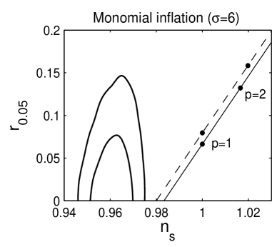
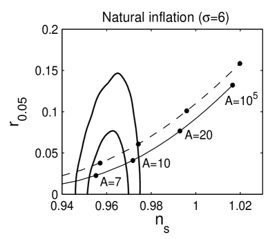
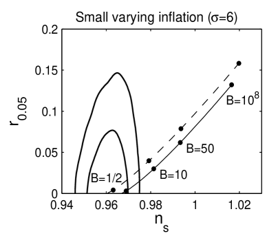
Figure 3: Two-dimensional observational constraints on non-commutative inflation with $\sigma=6$ in the ($n_{\rm s},r$) plane. Each panel corresponds to monomial inflation (top), natural inflation (middle), and small-varying inflaton models (bottom). The consistency relation $r=4n_{\rm t}$ is assumed. The two contours show the 68 % and 95 % CL boundaries. The solid and dashes curves represent the theoretical predictions of $n_{\rm s}$ and $r$ for $N=60$ and 50, respectively.

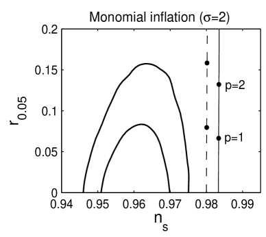
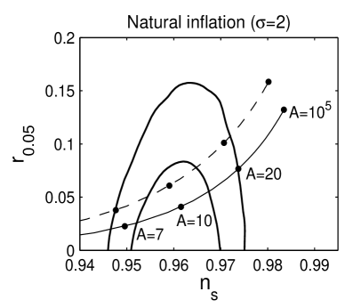
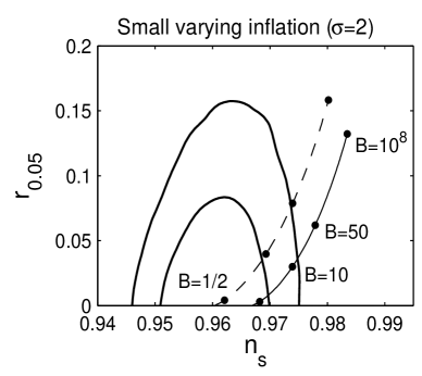
Figure 4: Two-dimensional observational constraints on non-commutative inflation with $\sigma=2$ in the ($n_{\rm s},r$) plane for monomial inflation (top), natural inflation (middle), and small-varying inflaton models (bottom). The meanings of observational contours and theoretical curves are the same as shown in Fig. 4.

For decreasing $A$, both $n_{\rm s}$ and $r$ get smaller. When $\sigma=6$ and $N=60$, for example, we have $n_{\rm s}=0.9856$ and $r=0.0627$ for $A=15$, $n_{\rm s}=0.9345$ and $r=0.0096$ for $A=5$. As we see in Figs. 4 and 4, there are some intermediate values of $A$ which are inside the 68 % CL observational contour. From the joint data analysis of Planck+WP+BAO+high-$\ell$, the parameter $A$ is constrained to be

$$5.9<A<11\quad(95\,\%\,{\rm CL})\quad{\rm for}~{}N=60~{}{\rm and}~{}\sigma=6\,,$$ (6.9)

$$5.8<A<9.9\quad(95\,\%\,{\rm CL})\quad{\rm for}~{}N=50~{}{\rm and}~{}\sigma=6\,,$$ (6.10)

and

$$6.5<A<20\quad(95\,\%\,{\rm CL})\quad{\rm for}~{}N=60~{}{\rm and}~{}\sigma=2\,,$$ (6.11)

$$7.0<A<23\quad(95\,\%\,{\rm CL})\quad{\rm for}~{}N=50~{}{\rm and}~{}\sigma=2\,.$$ (6.12)

When $N=80$, the constraints are $6.1<A<12\,(95\,\%\,{\rm CL})$ for $\sigma=6$ and $6.2<A<17\,(95\,\%\,{\rm CL})$ for $\sigma=2$. When $N=40$, we get $5.7<A<8.9\,(95\,\%\,{\rm CL})$ for $\sigma=6$ and $8.5<A<25\,(95\,\%\,{\rm CL})$ for $\sigma=2$. The bounds (6.9) and (6.11) translate to $0.84<f/m_{\rm Pl}<1.15$ and $0.88<f/m_{\rm Pl}<1.55$, respectively, whose parameter ranges are quite restrictive. Moreover, the symmetry-breaking scale $f$ cannot be much smaller than $m_{\rm Pl}$ as in the case of GR.

6.3 Small varying inflaton models

Finally, we study observational constraints on the potential (5.32). The end of inflation is characterized by $y_{\rm f}=(3B-\sqrt{6B})/(3B-2)$, where $y_{\rm f}=e^{-\alpha\phi_{\rm f}/m_{\rm Pl}}$ and $B=\beta_{1}^{2}m_{\rm Pl}^{2}/\alpha^{2}=8\pi/(3\alpha^{2})$. The Starobinsky model in the Einstein frame corresponds to $\alpha=4\sqrt{\pi/3}$, i.e., $B=1/2$. The number of e-foldings is

$$N=\frac{3B}{2}\left(\frac{1}{y}-\frac{1}{y_{\rm f}}+\ln\frac{y}{y_{\rm f}}\right),$$ (6.13)

whereas $n_{\rm s}$ and $r$ are

$$n_{\rm s} = 1-\frac{2}{3B}\frac{y(2y-\sigma y+2)}{(1-y)^{2}}\,,$$ (6.14)

$$r = \frac{32}{3B}\frac{y^{2}}{(1-y)^{2}}\,.$$ (6.15)

Expressing $y$ in terms of $N$ from Eq. (6.13), substituting it into Eqs. (6.14) and (6.15), and taking the limit $B\to\infty$, we obtain the values (6.4) and (6.5) with $p=2$. Therefore, this limit corresponds to the case of the quadratic potential, which lies outside the 95 % CL boundary for both $\sigma=2$ and 6. As can be seen in Figs. 4 and 4, the models enter the observationally allowed region for smaller $B$. If $\sigma=6$ and $N=60$, then $n_{\rm s}=0.9934$ and $r=0.0620$ for $B=50$, $n_{\rm s}=0.9814$ and $r=0.0299$ for $B=10$, and $n_{\rm s}=0.9689$ and $r=0.0030$ for $B=1/2$. The parameter $B$ is constrained to be

$$B<3.5\quad(95\,\%\,{\rm CL})\quad{\rm for}~{}N=60~{}{\rm and}~{}\sigma=6\,,$$ (6.16)

$$B<5.9\quad(95\,\%\,{\rm CL})\quad{\rm for}~{}N=50~{}{\rm and}~{}\sigma=6\,,$$ (6.17)

and

$$B<14\quad(95\,\%\,{\rm CL})\quad{\rm for}~{}N=60~{}{\rm and}~{}\sigma=2\,,$$ (6.18)

$$B<45\quad(95\,\%\,{\rm CL})\quad{\rm for}~{}N=50~{}{\rm and}~{}\sigma=2\,.$$ (6.19)

The model is excluded if $N>80$ both for $\sigma=6$ and $\sigma=2$. When $N=40$, we get $B<8.1\,(95\,\%\,{\rm CL})$ for $\sigma=6$ and $B<130\,(95\,\%\,{\rm CL})$ for $\sigma=2$.

The Starobinsky model in the Einstein frame ($B=1/2$) is inside the 68 % CL contour both for $\sigma=2$ and 6. The bounds (6.16) and (6.18) translate to $\alpha>1.55$ and $\alpha>0.77$, respectively. The models with $\alpha$ smaller than the order of 1 are disfavored because the cosmic acceleration relevant to CMB anisotropies occurs around the potential minimum.

7 Conclusions

We studied observational constraints on braneworld and non-commutative inflation in the light of the recent Planck data. The consistency relations between the tensor-to-scalar ratio $r$ and the tensor spectral index $n_{\rm t}$ are different depending on the scenario (RS braneworld, GB braneworld and two versions of non-commutative inflation). We ran the CosmoMC code for four different consistency relations and found that the likelihood results are similar to those obtained in GR ($r=-8n_{\rm t}$). We also confirmed that, under the slow-roll approximation, the scalar and tensor runnings can be set to 0 in the likelihood analysis.

For each class of braneworld and non-commutative inflation, we placed experimental constraints on a number of representative inflaton potentials such as (i) monomial inflation: $V(\phi)=V_{0}\phi^{p}$, (ii) natural inflation: $V(\phi)=V_{0}[1+\cos(\phi/f)]$, and (iii) small-varying inflaton models: $V(\phi)=V_{0}(1-e^{-\alpha\phi/m_{\rm Pl}})^{2}$.

In the RS braneworld, the monomial potential $V(\phi)=V_{0}\phi^{p}$ is outside the 95 % CL boundary for $p\geq 2$. The linear potential is marginally inside the 95 % CL border for $N=60$. The parameter $A_{\rm RS}=(4\pi/3)(V_{0}/\lambda)(f/m_{\rm Pl})^{2}$ in natural inflation is constrained to be $3.5<A_{\rm RS}<49$ (95 % CL) for $N=60$, so that a symmetry-breaking scale $f$ smaller than $m_{\rm Pl}$ can be allowed for $V_{0}/\lambda\gg 1$. We note, however, that the allowed parameter space is quite narrow for $N=50$, i.e., $5.0<A_{\rm RS}<11$ (95 % CL). In small-varying inflaton models, the observables are quantified by the parameter $B_{\rm RS}=(4\pi/3)(V_{0}/\lambda)(1/\alpha^{2})$. Since $n_{\rm s}$ and $r$ approach the values of the quadratic potential $V(\phi)=V_{0}\phi^{2}$ in the limit $B_{\rm RS}\to\infty$, the parameter $B_{\rm RS}$ is constrained to be $B_{\rm RS}<1650$ (95 % CL). In the Starobinsky model ($\alpha=4\sqrt{\pi/3}$), this translates into the condition $V_{0}/\lambda<6.6\times 10^{3}$.

In the GB braneworld, the monomial potential $V(\phi)=V_{0}\phi^{p}$ with $p>0$ lies outside the 95 % CL region for $N\geq 50$. In natural inflation, the parameter $A_{\rm GB}=\beta_{2/3}^{2}f^{2}V_{0}^{-1/3}$ is constrained to be $8.7<A_{\rm GB}<38$ (95 % CL) for $N=60$, whereas in small-varying inflaton models the bound on the parameter $B_{\rm GB}=\beta_{2/3}^{2}m_{\rm Pl}^{2}/(\alpha^{2}V_{0}^{1/3})$ is found to be $B_{\rm GB}<67$ (95 % CL) for $N=60$.

In non-commutative inflation with $\sigma=6$ and 2, the monomial potential $V(\phi)=V_{0}\phi^{p}$ ($p>0$) is outside the 99 % CL boundary because the scalar spectral index gets larger than in GR. In natural inflation, the parameter $A=(8\pi/3)(f/m_{\rm Pl})^{2}$ is constrained to be $5.9<A<11$ (95 % CL) for $\sigma=6$, $N=60$ and $6.5<A<20$ (95 % CL) for $\sigma=2$, $N=60$. Hence the symmetry-breaking scale $f$ is of the order of $m_{\rm Pl}$ as in the case of GR. In small-varying inflaton models, the bound on the parameter $B=8\pi/(3\alpha^{2})$ is given by $B<3.5$ (95 % CL) for $\sigma=6$, $N=60$ and $B<14$ (95 % CL) for $\sigma=2$, $N=60$, so that the Starobinsky model in the Einstein frame ($B=1/2$) is consistent with the data.

All these results have been also extended to values of $N$ smaller and larger than 50 and 60, depending on the details of the reheating stage. The corresponding bounds on the parameters of the inflationary potential (quoted in the text) are numerically different than those for $N=50,\,60$, but not enough to issue a qualitatively different physics.

Overall, braneworld and non-commutative models are not particularly favored over standard inflationary scenarios by CMB experiments. The viable parameter space in those models is not large enough to give any significant advantage with respect to their GR counterpart. We note that there are some models which give rise to $n_{\rm s}$ smaller than 0.94 —such as the minimal super-symmetric model [74], renormalizable-inflection-point inflation [75], tip inflation [76], and so on. There may be some possibilities that models with small $n_{\rm s}$ were rescued by braneworld and non-commutative effects due to the increase of $n_{\rm s}$. We leave the analysis of such specific inflaton potentials for future work, possibly after the 2-year data release of Planck.

References

- [1] D.N. Spergel et al. [WMAP Collaboration], First year Wilkinson Microwave Anisotropy Probe (WMAP) observations: Determination of cosmological parameters, Astrophys. J. Suppl. 148 (2003) 175 [astro-ph/0302209].
-
[2]
C.L. Bennett et al. [WMAP Collaboration], Nine-year Wilkinson Microwave Anisotropy Probe (WMAP) observations: final maps and results, Astrophys. J. Suppl. 208 (2013) 20 [arXiv:1212.5225];
G. Hinshaw et al. [WMAP Collaboration], Nine-year Wilkinson Microwave Anisotropy Probe (WMAP) observations: cosmological parameter results, Astrophys. J. Suppl. 208 (2013) 19 [arXiv:1212.5226]. - [3] P.A.R. Ade et al. [Planck Collaboration], Planck 2013 results. I. Overview of products and scientific results, arXiv:1303.5062.
- [4] P.A.R. Ade et al. [Planck Collaboration], Planck 2013 results. XXII. Constraints on inflation, arXiv:1303.5082.
- [5] J. Martin, C. Ringeval and V. Vennin, Encyclopaedia Inflationaris, arXiv:1303.3787.
- [6] Y.Z. Ma, Q.G. Huang and X. Zhang, Confronting brane inflation with Planck and pre-Planck data, Phys. Rev. D 87 (2013) 103516 [arXiv:1303.6244].
- [7] T. Suyama, T. Takahashi, M. Yamaguchi and S. Yokoyama, Implications of Planck results for models with local type non-Gaussianity, JCAP 06 (2013) 012 [arXiv:1303.5374].
- [8] K. Nakayama, F. Takahashi and T.T. Yanagida, Polynomial Chaotic Inflation in the Planck Era, Phys. Lett. B 725 (2013) 111 [arXiv:1303.7315].
- [9] A. Ijjas, P.J. Steinhardt and A. Loeb, Inflationary paradigm in trouble after Planck2013, Phys. Lett. B 723 (2013) 261 [arXiv:1304.2785].
- [10] S. Tsujikawa, J. Ohashi, S. Kuroyanagi and A. De Felice, Planck constraints on single-field inflation, Phys. Rev. D 88 (2013) 023529 [arXiv:1305.3044].
- [11] C. P. Burgess, M. Cicoli and F. Quevedo, String Inflation After Planck 2013, arXiv:1306.3512.
- [12] S. Bartrum, M. Bastero-Gil, A. Berera, R. Cerezo, R. O. Ramos and J. G. Rosa, The importance of being warm (during inflation), arXiv:1307.5868.
- [13] R. Maartens and K. Koyama, Brane-world gravity, Living Rev. Rel. 13 (2010) 5 [arXiv:1004.3962].
- [14] R. Brandenberger and P.-M. Ho, Noncommutative spacetime, stringy spacetime uncertainty principle, and density fluctuations, Phys. Rev. D 66 (2002) 023517 [hep-th/0203119].
- [15] L. Randall and R. Sundrum, Large mass hierarchy from a small extra dimension, Phys. Rev. Lett. 83 (1999) 3370 [hep-ph/9905221].
- [16] L. Randall and R. Sundrum, Alternative to compactification, Phys. Rev. Lett. 83 (1999) 4690 [hep-th/9906064].
- [17] J.E. Kim, B. Kyae and H.M. Lee, Effective Gauss–Bonnet interaction in Randall–Sundrum compactification, Phys. Rev. D 62 (2000) 045013 [hep-ph/9912344].
- [18] J.E. Kim, B. Kyae and H.M. Lee, Various modified solutions of the Randall–Sundrum model with the Gauss–Bonnet interaction, Nucl. Phys. B 582 (2000) 296 [Erratum-ibid. B 591 (2000) 587] [hep-th/0004005].
- [19] Q.-G. Huang and M. Li, CMB power spectrum from noncommutative spacetime, JHEP 0306 (2003) 014 [hep-th/0304203].
- [20] M. Fukuma, Y. Kono and A. Miwa, Effects of space-time noncommutativity on the angular power spectrum of the CMB, Nucl. Phys. B 682 (2004) 377 [hep-th/0307029].
- [21] S. Tsujikawa, R. Maartens and R. Brandenberger, Noncommutative inflation and the CMB, Phys. Lett. B 574 (2003) 141 [astro-ph/0308169].
- [22] Q.-G. Huang and M. Li, Noncommutative inflation and the CMB multipoles, JCAP 11 (2003) 001 [astro-ph/0308458].
- [23] Q.-G. Huang and M. Li, Power spectra in spacetime noncommutative inflation, Nucl. Phys. B 713 (2005) 219 [astro-ph/0311378].
- [24] H. Kim, G.S. Lee and Y.S. Myung, Noncommutative spacetime effect on the slow-roll period of inflation, Mod. Phys. Lett. A 20 (2005) 271 [hep-th/0402018].
- [25] H. Kim, G.S. Lee, H.W. Lee and Y.S. Myung, Second order corrections to noncommutative spacetime inflation, Phys. Rev. D 70 (2004) 043521 [hep-th/0402198].
- [26] R.-G. Cai, A Note on curvature fluctuation of noncommutative inflation, Phys. Lett. B 593 (2004) 1 [hep-th/0403134].
- [27] G. Calcagni, Noncommutative models in patch cosmology, Phys. Rev. D 70 (2004) 103525 [hep-th/0406006].
- [28] G. Calcagni, Consistency relations and degeneracies in (non)commutative patch inflation, Phys. Lett. B 606 (2005) 177 [hep-ph/0406057].
- [29] G. Calcagni and S. Tsujikawa, Observational constraints on patch inflation in noncommutative spacetime, Phys. Rev. D 70 (2004) 103514 [astro-ph/0407543].
- [30] A. Lukas, B.A. Ovrut, K.S. Stelle and D. Waldram, The Universe as a domain wall, Phys. Rev. D 59 (1999) 086001 [hep-th/9803235].
- [31] A. Lukas, B.A. Ovrut and D. Waldram, Cosmological solutions of Horava–Witten theory, Phys. Rev. D 60 (1999) 086001 [hep-th/9806022].
- [32] P. Binétruy, C. Deffayet and D. Langlois, Nonconventional cosmology from a brane universe, Nucl. Phys. B 565 (2000) 269 [hep-th/9905012].
- [33] P. Binétruy, C. Deffayet, U. Ellwanger and D. Langlois, Brane cosmological evolution in a bulk with cosmological constant, Phys. Lett. B 477 (2000) 285 [hep-th/9910219].
- [34] T. Shiromizu, K.-i. Maeda and M. Sasaki, The Einstein equation on the 3-brane world, Phys. Rev. D 62 (2000) 024012 [gr-qc/9910076].
- [35] D.J. Gross and J.H. Sloan, The quartic effective action for the heterotic string, Nucl. Phys. B 291 (1987) 41.
- [36] C. Charmousis and J.-F. Dufaux, General Gauss–Bonnet brane cosmology, Class. Quantum Grav. 19 (2002) 4671 [hep-th/0202107].
- [37] S.C. Davis, Generalized Israel junction conditions for a Gauss–Bonnet brane world, Phys. Rev. D 67 (2003) 024030 [hep-th/0208205].
- [38] E. Gravanis and S. Willison, Israel conditions for the Gauss–Bonnet theory and the Friedmann equation on the brane universe, Phys. Lett. B 562 (2003) 118 [hep-th/0209076].
- [39] K. Maeda and T. Torii, Covariant gravitational equations on brane world with Gauss-Bonnet term, Phys. Rev. D 69 (2004) 024002 [hep-th/0309152].
- [40] G. Calcagni, Slow-roll parameters in braneworld cosmologies, Phys. Rev. D 69 (2004) 103508 [hep-ph/0402126].
- [41] D.J. Schwarz, C.A. Terrero-Escalante and A.A. Garcia, Higher order corrections to primordial spectra from cosmological inflation, Phys. Lett. B 517 (2001) 243 [astro-ph/0106020].
- [42] S.M. Leach, A.R. Liddle, J. Martin and D.J. Schwarz, Cosmological parameter estimation and the inflationary cosmology, Phys. Rev. D 66 (2002) 023515 [astro-ph/0202094].
- [43] R. Maartens, D. Wands, B.A. Bassett and I. Heard, Chaotic inflation on the brane, Phys. Rev. D 62 (2000) 041301 [hep-ph/9912464].
- [44] D. Langlois, R. Maartens and D. Wands, Gravitational waves from inflation on the brane, Phys. Lett. B 489 (2000) 259 [hep-th/0006007].
- [45] A.R. Liddle and A.J. Smith, Observational constraints on brane world chaotic inflation, Phys. Rev. D 68 (2003) 061301 [astro-ph/0307017].
- [46] S. Tsujikawa and A.R. Liddle, Constraints on brane world inflation from CMB anisotropies, JCAP 03 (2004) 001 [astro-ph/0312162].
- [47] J.F. Dufaux, J.E. Lidsey, R. Maartens and M. Sami, Cosmological perturbations from brane inflation with a Gauss-Bonnet term, Phys. Rev. D 70 (2004) 083525 [hep-th/0404161].
- [48] S. Tsujikawa, M. Sami and R. Maartens, Observational constraints on braneworld inflation: The Effect of a Gauss-Bonnet term, Phys. Rev. D 70 (2004) 063525 [astro-ph/0406078].
- [49] T. Yoneya, Duality and indeterminacy principle in string theory, in Wandering in the Fields, K. Kawarabayashi and A. Ukawa (Eds.), World Scientific, Singapore (1987).
- [50] M. Li and T. Yoneya, D particle dynamics and the space-time uncertainty relation, Phys. Rev. Lett. 78 (1997) 1219 [hep-th/9611072].
- [51] T. Yoneya, String theory and space-time uncertainty principle, Prog. Theor. Phys. 103 (2000) 1081 [hep-th/0004074].
- [52] http://cosmologist.info/cosmomc/
- [53] A. Lewis, Efficient sampling of fast and slow cosmological parameters, Phys. Rev. D 87 (2013) 103529 [arXiv:1304.4473].
-
[54]
F. Beutler et al., The 6dF Galaxy Survey: baryon acoustic oscillations and the local Hubble constant, Mon. Not. Roy. Astron. Soc. 416 (2011) 3017 [arXiv:1106.3366];
N. Padmanabhan et al., A 2% distance to by reconstructing baryon acoustic oscillations – I: methods and application to the Sloan Digital Sky Survey, Mon. Not. Roy. Astron. Soc. 427 (2012) 2132 [arXiv:1202.0090];
L. Anderson et al., The clustering of galaxies in the SDSS-III Baryon Oscillation Spectroscopic Survey: baryon acoustic oscillations in the Data Release 9 Spectroscopic Galaxy Sample, Mon. Not. Roy. Astron. Soc. 427 (2013) 3435 [arXiv:1203.6594]. -
[55]
S. Das et al., The Atacama cosmology telescope: temperature and gravitational lensing power spectrum measurements from three seasons of data,
arXiv:1301.1037;
C.L. Reichardt et al., A measurement of secondary cosmic microwave background anisotropies with two years of South Pole Telescope observations, Astrophys. J. 755 (2012) 70 [arXiv:1111.0932]. - [56] J.M. Maldacena, Non-Gaussian features of primordial fluctuations in single field inflationary models, JHEP 05 (2003) 013 [astro-ph/0210603].
- [57] P. Creminelli and M. Zaldarriaga, Single field consistency relation for the 3-point function, JCAP 10 (2004) 006 [astro-ph/0407059].
- [58] A. De Felice and S. Tsujikawa, Shapes of primordial non-Gaussianities in the Horndeski’s most general scalar-tensor theories, JCAP 03 (2013) 030 [arXiv:1301.5721].
- [59] P.A.R. Ade et al. [Planck Collaboration], Planck 2013 Results. XXIV. Constraints on primordial non-Gaussianity, arXiv:1303.5084.
- [60] G. Calcagni, Non-Gaussianity in braneworld and tachyon inflation, JCAP 10 (2005) 009 [astro-ph/0411773].
- [61] B.M. Murray and Y.S. Myung, Gauss–Bonnet braneworld and WMAP three year results, Phys. Lett. B 642 (2006) 426 [astro-ph/0605684].
- [62] M.C. Bento, R. González Felipe and N.M.C. Santos, Braneworld inflation from an effective field theory after WMAP three-year data, Phys. Rev. D 74 (2006) 083503 [astro-ph/0606047].
- [63] A. Bouaouda, R. Zarrouki, H. Chakir and M. Bennai, -term braneworld inflation in light of five-year WMAP observations, Int. J. Mod. Phys. A 25 (2010) 3445 [arXiv:1010.4884].
- [64] K. Nozari and N. Rashidi, Non-minimal braneworld inflation after Planck, arXiv:1309.1950.
- [65] N. Li and X. Zhang, Reexamination of inflation in noncommutative space-time after Planck results, Phys. Rev. D 88 (2013) 023508 [arXiv:1304.4358].
- [66] A.R. Liddle and S.M. Leach, How long before the end of inflation were observable perturbations produced?, Phys. Rev. D 68 (2003) 103503 [astro-ph/0305263].
- [67] E.J. Copeland and O. Seto, Reheating and gravitino production in braneworld inflation, Phys. Rev. D 72 (2005) 023506 [hep-ph/0505149].
- [68] A.D. Linde, Chaotic inflation, Phys. Lett. B 129 (1983) 177.
-
[69]
E. Silverstein and A. Westphal,
Monodromy in the CMB: gravity waves and string inflation,
Phys. Rev. D 78 (2008) 106003 [arXiv:0803.3085];
L. McAllister, E. Silverstein and A. Westphal, Gravity waves and linear inflation from axion monodromy, Phys. Rev. D 82 (2010) 046003 [arXiv:0808.0706]. -
[70]
F. Lucchin and S. Matarrese, Power-law inflation, Phys. Rev. D 32 (1985) 1316;
J.J. Halliwell, Scalar fields in cosmology with an exponential potential, Phys. Lett. B 185 (1987) 341;
Y. Kitada and K.-i. Maeda, Cosmic no-hair theorem in power-law inflation, Phys. Rev. D 45 (1992) 1416. -
[71]
K. Freese, J.A. Frieman and A.V. Olinto, Natural inflation with pseudo Nambu–Goldstone bosons, Phys. Rev. Lett. 65 (1990) 3233;
F.C. Adams, J.R. Bond, K. Freese, J.A. Frieman and A.V. Olinto, Natural inflation: particle physics models, power-law spectra for large-scale structure, and constraints from COBE, Phys. Rev. D 47 (1993) 426 [hep-ph/9207245]. - [72] A.A. Starobinsky, A new type of isotropic cosmological models without singularity, Phys. Lett. B 91 (1980) 99.
-
[73]
K.-i. Maeda, Towards the Einstein–Hilbert action via conformal transformation, Phys. Rev. D 39 (1989) 3159;
A. De Felice and S. Tsujikawa, theories, Living Rev. Rel. 13 (2010) 3 [arXiv:1002.4928]. - [74] R. Allahverdi, K. Enqvist, J. García-Bellido and A. Mazumdar, Gauge invariant MSSM inflaton, Phys. Rev. Lett. 97 (2006) 191304 [hep-ph/0605035].
- [75] R. Allahverdi, B. Dutta and A. Mazumdar, Unifying inflation and dark matter with neutrino masses, Phys. Rev. Lett. 97 (2007) 261301 [arXiv:0708.3983].
- [76] L. Lorenz, J. Martin and C. Ringeval, Brane inflation and the WMAP data: a Bayesian analysis, JCAP 08 (2008) 04 [arXiv:0709.37584].