Spin polarization oscillations in a magnetically inhomogeneous conducting ring

Abstract

The real part of the conductance of a 1D conducting ring with magnetic properties that vary along the conductor is examined. The possibility of exciting a new type of spin polarization oscillations in the ring with an external emf is analyzed.

It has been shown ref1 ; ref2 ; ref3 that new, weakly damped spin polarization waves which may be accompanied by electric current oscillations, can exist in micro-sized magnetic conductors and their frequency can be controlled over a wide range through variations in external parameters. This sort of “spin pendulum” may be regarded as another spintronic device ref4 . Combined oscillations of the spin concentration and drift current in conducting magnetic rings have been examined ref1 ; ref2 under conditions corresponding to electron hydrodynamics ref5 . These oscillations can exist only in a ring with spatially inhomogeneous magnetic properties: The equilibrium densities of the spin components $n_{\uparrow}$ and $n_{\downarrow}$ (“spin-up” and “spindown” electrons) must vary along the ring. Magnetic inhomogeneity can be produced, for example, in conducting heterostructures ref6 by means of a nonuniform electrical gate potential.

The existence of a different type of oscillations in the spin density under ballistic electron transport conditions in rings and open circuits has been pointed out ref3 . These oscillations should be most marked in one-dimensional conductors, i.e., wires that are so thin that only one conductivity channel undergoes spatial quantization. These oscillations are similar to beam waves ref7 in metals with several groups of charge carriers. Electrical neutrality during ballistic transport by electrons with a nonequilibrium spin density $\rho_{\uparrow,\downarrow}$ (the total charge density of the spin components is $n_{\uparrow,\downarrow}+\rho_{\uparrow,\downarrow}$) is achieved by meeting the condition $\rho_{\uparrow}=-\rho_{\downarrow}$. (Here and in the following we are considering one-dimensional densities.) These oscillations do not require magnetic inhomogeneity of the wire; they are possible both in magnetic and nonmagnetic materials. However, as shown below, they can be excited by an electric field only in the magnetically nonuniform case. As opposed to spin waves in metals ref8 , the spin polarization oscillations predicted in ref3 exist even when there is no spin dependent Fermi-liquid interaction.

This paper examines the excitation of all oscillations of this type in magnetically inhomogeneous rings with an arbitrary relation between the frequencies of collisions with and without momentum loss and the frequency of the oscillations. We consider a ring consisting of a 1D conductor whose magnetic inhomogeneity is modelled as two homogeneous magnets with lengths $L_{l}$ and $L_{r}$ Fig.1 with equilibrium densities $n_{\uparrow,\downarrow l}$ and $n_{\uparrow,\downarrow r}$, respectively, of the spin components in the “left” and “right” parts of the ring. This model has been chosen in order to simplify the calculations and it is not necessary to join two different magnets in an experiment. A contact potential barrier usually develops at a junction and this is not present in our analysis. The directions of the magnetization are assumed collinear at all points in the ring, so that there are no coherence effects in the magnetic components.

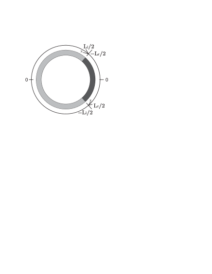
Figure 1: A conducting ring consisting of two parts with different magnetic properties.

The quasiclassical equations for the drift velocities of the electron components $u_{\uparrow,\downarrow}$ and the increments in their densities $\rho_{\uparrow,\downarrow}$ in the ballistic limit for a 1D conductor are given in ref2 . Relaxation phenomena in a magnet can be taken into account using the Flensberg approximation ref9 , as done in ref10 . We then have the following system of equations:

$$\frac{\partial\rho_{\sigma}}{\partial t}+j_{\sigma}^{\prime}=-\frac{e\Pi_{0}}{\tau_{sf}}\left(\mu_{\sigma}-\mu_{-\sigma}\right)$$ (1)

$$\frac{m}{n_{\sigma}}\frac{\partial j_{\sigma}}{\partial t}+\left(\mu_{\sigma}+e\varphi\right)^{\prime}-eE=-\sum_{\sigma^{\prime}}\beta_{\sigma\sigma^{\prime}}j_{\sigma^{\prime}}$$ (2)

$$\begin{split}\beta_{\uparrow\uparrow}=e(\rho_{i\uparrow}+An_{\uparrow}^{-2}),\;\beta_{\downarrow\downarrow}=e(\rho_{i\downarrow}+An_{\downarrow}^{-2}),\\ \beta_{\uparrow\downarrow}=\beta_{\downarrow\uparrow}=-eA(n_{\uparrow}n_{\downarrow})^{-1}\end{split}$$ (3)

$$\sum_{\sigma}\rho_{\sigma}=0$$ (4)

These equations hold for a degenerate electron system in an approximation that is linear with respect to the deviation from equilibrium. The subscript $\sigma$ enumerates the spin direction ($-\sigma$ is opposite to $\sigma$); $j_{\sigma}=n_{\sigma}u_{\sigma}$ is the electric current of the spin component; $\Pi_{0}^{-1}=\Pi_{\uparrow}^{-1}+\Pi_{\downarrow}^{-1}$, where $\Pi_{\sigma}$ is the density of states at the Fermi level; $\tau_{sf}$ is the lifetime with respect to spin flip of the electrons; the masses of the electrons for both components are assumed for simplicity to be the same and equal to $m$; $\varphi$ is the potential of the electric field that develops with electron disequilibrium; $e$ is the electronic charge; and, $\mu_{\sigma}$ is the nonequilibrium increment to the chemical potential, given in the linear approximation by

$$\rho_{\sigma}=e\Pi_{\sigma}\mu_{\sigma}$$ (5)

The $\beta_{\sigma\sigma^{\prime}}$ describe the electron relaxation processes: $\rho_{i}$ is the specific resistance associated with momentum-loss electron collisions (e.g., collisions with impurities) and the constant $A$ is proportional to the electron-electron collision frequency $\nu_{ee}$ ($A\approx e^{-1}m\nu_{ee}n_{m},\;n_{m}^{-1}=n_{\uparrow}^{-1}+n_{\downarrow}^{-1}$) with conservation of the momentum of the electron system.

We consider the excitation of spin density oscillations in the ring by an electric induction field $E=E_{0}e^{i\omega t}$ created by the flux of an external variable magnetic field through the area of the ring. We limit ourselves to linear oscillations, so in the following we assume that

$$\rho_{\uparrow,\downarrow}(x,t)=\rho_{\uparrow,\downarrow}(x)e^{i\omega t},$$

$$j_{\uparrow,\downarrow}(x,t)=j_{\uparrow,\downarrow}(x)e^{i\omega t}.$$

For further calculations it is convenient to reduce Eq. (1) to the following form using Eqs. (4) and (5):

$$e\Pi_{\sigma}\mu_{\sigma}\left(i\omega+\tau_{sf}^{-1}\right)+j_{\sigma}^{\prime}=0$$ (6)

We write Eq. (2) as

$$\gamma_{\sigma}j_{\sigma}-aj=-\frac{\mu_{\sigma}^{\prime}}{e}-\varphi^{\prime}+E$$ (7)

where

$$\gamma_{\sigma}=\frac{i\omega m}{en_{\sigma}}+\rho_{i\sigma}+\frac{A}{n_{\sigma}^{2}}+\frac{A}{n_{\sigma}n_{-\sigma}},\,a=\frac{A}{n_{\sigma}n_{-\sigma}},\,j=j_{\uparrow}+j_{\downarrow}.$$

Let the points $x=0$ lie in the middle of both parts, as shown in 1. Then the solution of Eqs. (6) and (7) can be conveniently sought in the form

$$j_{\sigma}(x)=d_{\sigma}+f_{\sigma}\left(e^{-x/\lambda}+\alpha e^{x/\lambda}\right)$$

$$\mu_{\sigma}(x)=g_{\sigma}\left(e^{-x/\lambda}-\alpha e^{x/\lambda}\right)$$

$$\varphi(x)=b+cx+h\left(e^{-x/\lambda}-\alpha e^{x/\lambda}\right).$$

The computations are greatly simplified because of the symmetry of the equations for $j_{\sigma}$, $\mu_{\sigma}$, $\varphi$ with respect to the substitution $x\rightarrow-x$. The symmetry means that for all solutions (if they exist) the coefficient $\alpha$ can be chosen to have values of $\alpha=\pm 1$. If $E\neq 0$ (induced oscillations), then choosing $\alpha=-1$ does not correspond to symmetry of the induced force in Eq. (2). Thus, the way of exciting oscillations with an electric field considered here only yields eigenmodes that are symmetric with respect to the coordinate origin in Fig. 1. Setting $\alpha=1$, substituting the currents and potentials in Eqs.(6) and (7), and equating (separately) the free constants and preexponential factors, for each part of the ring we obtain the system of equations

$$e\Pi_{\sigma}\left(i\omega+\tau_{sf}^{-1}\right)g_{\sigma}=\frac{f_{\sigma}}{\lambda}$$

$$\gamma_{\sigma}f_{\sigma}=\frac{1}{e\lambda}\left(g_{\sigma}+eh\right)$$

$$\gamma_{\sigma}d_{\sigma}-aj=c+E.$$

The condition of electrical neutrality (4) and the continuity equation (1) imply that the total current $j$ is independent of position, so that $f_{\sigma}=-f_{-\sigma}$. The first and second of these equations form a system of homogeneous equations for $f$, $\mu_{\sigma}$ and $\varphi$. This system of equations has a nontrivial solution for $\lambda$ such that

$$\lambda^{2}=\left(e\Pi_{0}\left(i\omega+\tau_{sf}^{-1}\right)\gamma\right)^{-1},$$ (8)

where $\gamma=\gamma_{\uparrow}+\gamma_{\downarrow}$. The third of these equations can be used to express the constants $d_{\sigma}$ in terms of the total current $j$,

$$d_{\sigma}=j\frac{\gamma_{-\sigma}}{\gamma}.$$ (9)

The constants corresponding to the different parts of the ring are coupled by the continuity conditions for the spin currents and the conditions for the electrochemical potentials at the two boundaries in the ring. Since the symmetry of the problem is already taken into account in writing down these quantities, it is sufficient to write down the matching conditions at one of the two boundaries:

$$j_{l\sigma}(-L_{l}/2)=j_{r\sigma}(L_{r}/2)$$

$$\mu_{l\sigma}(-L_{l}/2)+e\varphi_{l}(-L_{l}/2)=\mu_{r\sigma}(L_{r}/2)+e\varphi_{r}(L_{r}/2).$$

The above system of equations can be used to express the constants $f_{\sigma}$ in terms of the constants $d_{\sigma}$:

$$f_{l,r\sigma}=\frac{(d_{r,l\sigma}-d_{l,r\sigma})(1-N_{r,l})\gamma_{r,l}\lambda_{r,l}e^{-L_{l,r}/2\lambda_{l,r}}}{(1+N_{l})(1-N_{r})\gamma_{r}\lambda_{r}+(1+N_{r})(1-N_{l})\gamma_{l}\lambda_{l}},$$ (10)

$$N_{l,r}=e^{-L_{l,r}/\lambda_{l,r}}.$$

Substituting Eq. (10) in Eq. (7), using Eq. (9) for this, and integrating the resulting equation over the entire ring, we obtain the relationship between the total current $j$ and the external emf $\oint Edx$:

$$\oint Edx=Rj$$ (11)

$$R=R_{l}+R_{r}+2R_{border}$$ (12)

$$R_{l,r}=L_{l,r}\left(\frac{\gamma_{\uparrow\,l,r}\gamma_{\downarrow\,l,r}}{\gamma_{l,r}}-a\right)$$ (13)

$$R_{border}=\frac{(1-N_{l})(1-N_{r})(\gamma_{\downarrow\,l}\gamma_{\uparrow\,r}-\gamma_{\downarrow\,r}\gamma_{\uparrow\,l})^{2}}{\gamma_{l}^{2}\gamma_{r}^{2}\left(\displaystyle{\frac{(1+N_{l})(1-N_{r})}{\lambda_{l}\gamma_{l}}+\frac{(1+N_{r})(1-N_{l})}{\lambda_{r}\gamma_{r}}}\right)}.$$ (14)

Equation (13) gives the resistances of the two parts of the ring in the absence of a spin disequilibrium; thus, $R_{border}$ is related to the magnetic inhomogeneity of the ring. If we set $\omega=0$, $N_{l,r}=0$, then Eq. (14) is exactly equal to the nonequilibrium resistance of a single boundary between two wires with different magnetic properties obtained in Ref. ref11 . In the following we shall be interested in the dependence of the real part of the conductance of the ring on the frequency $\omega$ of the external emf i.e., $Z(\omega)=\mathrm{Re}(1/R(\omega))$.

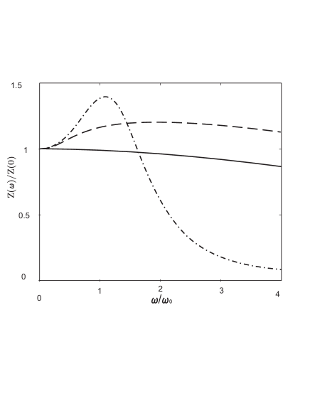
Figure 2: The function $Z(\omega)/Z(0)$ constructed using Eq. (12) for a ring consisting of two parts of equal length ($L_{l}=L_{r}$). The frequency is measured in units of the characteristic frequency $\omega_{0}^{2}=\displaystyle{\frac{n_{\uparrow}n_{\downarrow}}{mne\Pi_{0}L^{2}}}\approx\displaystyle\frac{v_{F}^{2}}{L^{2}}$ of the system. The smooth and dashed curves correspond to the case where the frequencies of normal collisions and collisions with momentum loss of the electron system are 10 times the characteristic frequency ($\nu_{ee}=\nu_{i}=10\omega_{0}$). The smooth curve is for a magnetically homogeneous ring ($n_{l\uparrow\downarrow}=n_{r\uparrow\downarrow}$) and the dashed curve, for a magnetically inhomogeneous ring ($n_{l\uparrow\downarrow}=n_{r\downarrow\uparrow}$) with polarization $n_{\uparrow}/n_{\downarrow}=30/70$ of the electron density. The dot-dashed curve corresponds to the case of a magnetically inhomogeneous ring ($n_{l\uparrow\downarrow}=n_{r\downarrow\uparrow}$) with polarization $n_{\uparrow}/n_{\downarrow}=30/70$ of the electron density and an electron-electron collision frequency a factor of 10 times higher than the frequency of collisions with momentum loss by the electron system ($\nu_{ee}=10\omega_{0}$, $\nu_{i}=\omega_{0}$). In all cases the spin flip frequency is $\tau_{sf}^{-1}=\omega_{0}/10$

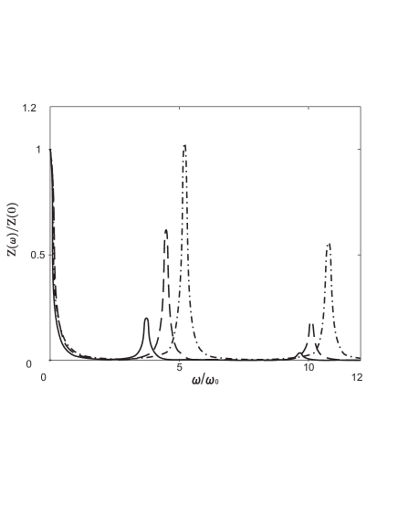
Figure 3: The function $Z(\omega)/Z(0)$ constructed using Eq. (12) for a ring consisting of two parts of equal length ($L_{l}=L_{r}$). The frequency is measured in units of the characteristic frequency $\omega_{0}^{2}=\displaystyle{\frac{n_{\uparrow}n_{\downarrow}}{mne\Pi_{0}L^{2}}}\approx\displaystyle\frac{v_{F}^{2}}{L^{2}}$ of the system, and the polarization $n_{\uparrow}/n_{\downarrow}$ of the electron density is $20/80$ for the smooth curve, $10/90$ for the dashed curve, an $5/95$ for the dot-dashed curve. The frequencies of normal collisions, collisions with momentum loss by the electronic system, and spin flip are each a factor of 10 times smaller than the characteristic frequency of the system, i.e., ($\nu_{ee}=\nu_{i}=\tau_{sf}^{-1}=\omega_{0}/10$).

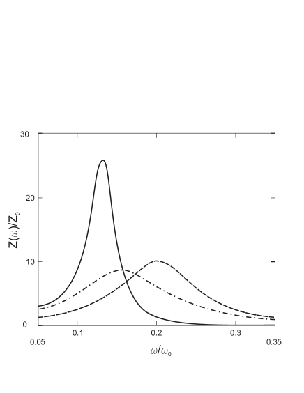
Figure 4: The function $Z(\omega)/Z_{0}$ constructed using Eq. (18) for a magnetically inhomogeneous ring with a smooth change in its magnetic properties. The frequency of normal collisions is $\nu_{ee}=1000\omega_{0}$ and there are no spin-flip processes or collisions with loss of momentum by the electron system. $Z_{0}^{-1}=\displaystyle{\oint\frac{m\omega_{0}}{ne^{2}}dx}$. $L_{tr}=0.2L$ for the smooth curve, $L_{tr}=0.05L$ for the dashed curve, and $L_{tr}=0.0125L$ for the dot-dashed curve, where $L$ is the length of the ring and $L_{tr}$ is the characteristic size of the magnetic inhomogeneity.

Figure 2 shows that a magnetic inhomogeneity of the ring makes $Z(\omega)$ increase with rising frequency for small $\omega$, while $Z(\omega)$ for a magnetically homogeneous ring decreases monotonically as the external frequency is raised. The increased conductance at low frequencies for a magnetically inhomogeneous sample can be explained in terms of the results of Ref. ref11 : since a spin inhomogeneity leads to increased electrical resistance in static conductivity ref11 , a frequency increase that limits the disequilibrium region in accordance with Eq. (8), will increase the conductance. The subsequent reduction in the conductance with increasing frequency is explained (as in the case of a uniform ring) by the inertia of the charge carriers, in accordance with the Drude-Lorentz formula. This rise in the conductance at frequencies that are low compared to $\omega_{0}$ occurs when $\nu_{i}+\nu_{ee}>\omega_{0}>>\tau_{sf}^{-1}$.

The characteristic maximum in Fig. 2 for a hydrodynamic conductivity corresponds to a “spin pendulum” resonance near the characteristic frequency ref1 . However, as opposed to Refs. ref1 ; ref2 ; ref3 , where a smooth variation in the magnetic properties of the ring was assumed, when there are sharp boundaries between regions with different magnetic properties the eigenmodes of the “spin pendulum” will be highly damped owing to diffusive processes near the boundaries and the damping constant will be on the order of the resonance frequency itself.

It should also be noted that the different mean free paths for collisions with impurities by the spin groups in a magnet ref12 can also affect the character of the resonance peaks. Thus, if the electron spin group with the lowest density scatters on impurities more often than electrons from another group, then the resonance peaks will be more distinct than when the scattering by electrons from the different spin groups is the same.

In the limit of ballistic transport in the ring, when the mean free path of the electrons for any collisions is much greater than the length of the ring, i.e., $\nu_{ee},\nu_{i}<<v_{F}/L$, and the spin relaxation time is much longer than the characteristic time for passage of an electron around the ring, i.e., $\tau_{sf}>>L/v_{F}$, the behavior of the conductance of a magnetically inhomogeneous ring differs substantially from the diffusive or hydrodynamic cases. Instead of a single resonance maximum in $Z(\omega)$, there are a number of resonances (Fig. 3) which are more distinct when the relaxation frequencies are lower. As in the case of diffusive transport, the resonances show up more distinctly if the magnetic inhomogeneity of the ring is greater. For the case in which both parts of the ring have the same length, $L_{l}=L_{r}$, the “left” and “right” parts are oppositely polarized ($n_{l\uparrow\downarrow}=n_{r\downarrow\uparrow}$), and are also weak, i.e., $|n_{\uparrow}-n_{\downarrow}|/n<<1$, with $\Pi_{0}=Const$, it is possible to find the resonance frequencies $\omega$ analytically. To do this, we set $\rho_{i\uparrow\downarrow}=0$ and $A=0$ in Eqs. (13) and (14), and then solve the equation $R(\omega)=0$. As a result, we obtain the following expression for the resonance frequencies:

$$\begin{split}\omega=\omega_{0}\left(1-\frac{\delta}{8}\right)\left(\pi+2\pi k+\frac{2\delta}{\pi+2\pi k}\right),\\ \delta=4\frac{(n_{\uparrow}-n_{\downarrow})^{2}}{n^{2}}<<1\end{split}$$ (15)

$$\omega_{0}=\frac{1}{2}\sqrt{\frac{n}{me\Pi_{0}L^{2}}},\,k=0,1,2\dots$$

As can be seen from Eq. (14), $R_{border}=0$ at all frequencies if the ratio $\gamma_{\uparrow}/\gamma_{\downarrow}$ is independent of position, i.e., under this condition all the above described features of the conductance are absent. This situation occurs with a homogeneous ring, but also if the inhomogeneity is not “magnetic”, i.e., if the densities of the spin components and their specific conductivities $\rho_{i}$ vary from point to point in proportion to one another. Thus, we have proved that oscillations can be excited by an electric field in a magnetically inhomogeneous ring. It is in just this case that spin density waves are accompanied by a variable electric current along the ring. The relationship between the spin oscillations and the current can be explained qualitatively as follows: the electrical neutrality condition makes the inhomogeneous concentrations of the two different spin components move together along the wire. When the conductivity of the components is nonuniform this is achieved through the appearance in the wire of an internal electric field, which creates a current.

It should be kept in mind that the roots of the equation $R(\omega)=0$ do not determine the frequencies of all the eigenmodes of the system, but only of those which can be excited by this electrical mechanism. Oscillations with current that are odd in x were mentioned above; they are not excited by an electric field, but are solutions of the system of Eqs. (4) - (7) without collisions and with $E=0$. The frequencies of these eigenmodes are

$$\omega=\omega_{0}\left(1-\frac{\delta}{8}\right)\left(2\pi k+\frac{\delta}{\pi k}\right).$$

Oscillations that are even in $x$ and odd in $x$ also exist in the ballistic regime in a homogeneous ring ($\delta=0$).

Since a sharp transition between magnetically homogeneous parts of the ring leads to rapid damping of “spin pendulum” waves, it is clear that a smooth transition leads to the most important changes in the case of hydrodynamic transport. In order to follow these changes, we introduce a finite transition length $L_{tr}<<L$ and let $\nu_{ee}>>\omega_{0}$, while neglecting collisions that do not conserve momentum and spin. We distinguish a purely hydrodynamic part of the currents which corresponds to equality of the drift velocities of the components:

$$j_{\sigma}=j\frac{n_{\sigma}}{n}\pm j_{1},$$

where the “+” sign corresponds to spin-up and “-” to spindown. Subtracting Eq. (7) for one component from the other for the different components, solving the resulting equation for $j_{1}$, and substituting in Eq. (1), we obtain

$$\frac{\partial\rho_{\uparrow}}{\partial t}=\left[\frac{n_{0}}{A}\left(\frac{\rho_{\uparrow}}{\Pi_{0}}\right)^{\prime}\right]^{\prime}-j\left(\frac{n_{\uparrow}}{n}\right)^{\prime},$$ (16)

where $n_{0}^{-1}=n_{\uparrow}^{-1}+n_{\downarrow}^{-1}$. Equation (16) describes the diffusion of the nonequilibrium spins near the transition, where the flowing current generates a spin disequilibrium. We simplify the model by assuming that $n_{0}$, $\Pi_{0}$ and $A$ are independent of $x$. Then we have

$$\mu_{\sigma}(x)=-\frac{j}{\Pi_{\sigma}}\int G(x-y)\left(\frac{n_{\uparrow}(y)}{n(y)}\right)^{\prime}dy,$$ (17)

where the Green function for the diffusion equation (16) is

$$G(x)=\frac{1}{2i\omega\lambda}e^{-|x|/\lambda},\,\lambda=\sqrt{\frac{n_{0}^{2}}{i\omega A\Pi_{0}}}.$$

In order to obtain an expression for the resistance $R$ in this case, we multiply both parts of Eqs. (7) by $n_{\sigma}$, add the equations for the different components (the terms with $A$ drops out of this sum), divide by $n$, and integrate over the entire ring. After integration by parts and using Eq. (17), we have

$$R=\frac{1}{e^{2}}\oint\left[\frac{i\omega m}{n}-\right.\\ \left.\frac{1}{\Pi_{0}}\int\left(\frac{n_{\uparrow}(x)}{n(x)}\right)^{\prime}G(x-y)\left(\frac{n_{\uparrow}(y)}{n(y)}\right)^{\prime}dy\right]dx.$$ (18)

When $\lambda<<L_{tr}$ the function $G(x-y)$ in Eq. (18) can be replaced by $(i\omega)^{-1}\delta(x-y)$ and the condition $R=0$ then gives the frequency of the oscillations of the “spin pendulum” found in Ref. ref1 :

$$\omega^{2}={\displaystyle\oint{\left(\frac{n_{\uparrow}}{n}\right)^{\prime}}^{2}\frac{1}{\Pi_{0}}dx}\left(\displaystyle\oint\frac{m}{n}dx\right)^{-1}.$$ (19)

Figure 4 is a plot of the function $Z(\omega)$ for a ring consisting of two oppositely magnetized parts of equal lengths with smooth transition regions of length $L_{tr}$ between them, constructed using Eq. (18) for three different values of $L_{tr}$. The graphs were constructed assuming weak magnetization of the ring ($|n_{\uparrow}-n_{\downarrow}|/n=0.035$) so that $\lambda$ could be treated as independent of $x$. It can be seen that the most distinct conductance peak occurs with the smoothest variation in the magnetic properties of the ring. This is explained by the fact that the period of the eigenmodes in this case is shorter than the time for the spin disequilibrium to diffuse through the region of $L_{tr}$. When the length of the transition between the halves of the rings with their different magnetic properties is reduced, the frequency of the resonance initially increases in accordance with the formula for the eigenfrequency (19) of the “spin pendulum” and ceases to increase when the “spin pendulum” frequency approaches $\tau_{d}^{-1}$, where $\tau_{d}\approx L_{tr}^{2}/D$ is the diffusion time for the spin disequilibrium in the region $L_{tr}$ and $D\approx v_{F}^{2}/\nu_{ee}\approx\omega_{0}^{2}L^{2}/\nu_{ee}$ is the diffusion coefficient.

We now estimate the characteristic order of magnitude of these oscillations in the ballistic frequency regime, $\omega_{0}\approx v_{F}/L$. Since the mean free path for collisions with structural imperfections in AsGa heterostructures is as long as 10 $\mu$ and $v_{F}\approx 10^{7}$ cm/s, we have $\omega_{0}\approx 10^{10}s^{-1}$. The frequency of the oscillations of the “spin pendulum” (hydrodynamic regime) can be significantly lower than $\omega_{0}$, since it contains the degree of inhomogeneity, $(n_{\uparrow}/n)_{r}-(n_{\uparrow}/n)_{l}$, as a reducing factor.

In this paper we have examined the frequency dependence of the resistance of magnetically inhomogeneous closed conductors. It has been shown that, depending on how the real part of the conductance of the ring depends on the frequency of an external emf, there can be a single maximum (in the case of diffusive or hydrodynamic transport) or a number of sharp peaks (in the case of ballistic transport) corresponding to excitation of eigenmodes of the spin polarization in the conductor by the external field. In the hydrodynamic case, the most distinct conductance maximum can be observed in rings with smoothly varying magnetic properties (“spin pendulum”).

The author thanks A. I. Kopeliovich for continuing interest in this work and valuable comments.

Translated by D. H. McNeill.

References

• (1) R.N.Gurzhi, A.N.Kalinenko, A.I.Kopeliovich, P.V.Pyshkin, A.V.Yanovsky, Phys. Rev. B 73, 153204 (2006).
• (2) R. N. Gurzhi, A. N. Kalinenkov, A. I. Kopeliovich, P. V. Pyshkin, and A.V. Yanovskii, ZhETF 132, 209 (2007).
• (3) R.N.Gurzhi, A.N.Kalinenko, A.I.Kopeliovich, P.V.Pyshkin, S.B.Rutkevich, A.V.Yanovsky, A.N.Yashin, Nonlinear Phenomena in Complex Systems, vol.10,#3, pp 238-246 (2007)
• (4) I. Zฬ†utiฤ‡, J. Fabian, and S. Das Sarma, Rev. Mod. Phys., 76, 323 (2004)
• (5) R. N. Gurzhi, UFN 94 (4), 689 (1968).
• (6) T. Ando et al., Review of Modern Physics, vol. 54, No. 2, p. 437-458 (1982)
• (7) Yu. A. Avramenko, E. V. Bezuglyi, N. G. Burma, and V. D. Fil, Low Temp. Phys. 35, 724 (2009).
• (8) E. M. Lifshitz and L. P. Pitaevskii, Statistical Physics, Part 2. Theory of the Condensed State (in Russian), Nauka, Moscow, 1978.
• (9) K. Flensberg, T.S. Jensen, N.A.Mortensen, Phys. Rev. B, 64, 245308 (2001)
• (10) A. I. Kopeliovich and P. V. Pyshkin, Low Temp. Phys. 35, 426 (2009)
• (11) R.N.Gurzhi, A.N.Kalinenko, A.I.Kopeliovich, P.V.Pyshkin, A.V.Yanovsky, Low Temp. Phys. 37, 149 (2011)
• (12) Bruce A. Gurney, Virgil S. Speriosu, Jean-Pierre Nozieres, Harry Lefakis, Dennis R. Wilhoit, and Omar U. Need, Phys. Rev. Lett. 71, 4023?4026 (1993)