Strong field electrodynamics of a thin foil

Abstract

Exact solutions describing the nonlinear electrodynamics of a thin double layer foil are presented. These solutions correspond to a broad range of problems of interest for the interaction of high intensity laser pulses with overdense plasmas such as frequency upshifting, high order harmonic generation and high energy ion acceleration.

I Introduction

High power laser irradiation of various targets, such as solid, cluster or gas targets, has been used for a number of years in order to study a broad range of mechanisms of high energy ion and electron acceleration ion-rev ; ele-rev , high and low energy photon generation photon-rev1 ; photon-rev2 ; photon-rev3 , and to explore problems of interest for modeling processes relevant to fundamental physics MTB ; fund-rev and astrophysics astro-rev .

When a high-intensity laser pulse interacts with a very thin foil target, which can be modelled as a thin slab of overdense plasma, features appear that are not encountered either in underdense or in overdense plasmas as noted in the current literature, see e.g., Refs. Foil1 ; MTB . These features provide novel regimes for ion acceleration IONS ; IONS-UL ; AAMS ; MacchiPRLReflectivity ; BulanovOptimalShape , relativistic high order harmonics generation RelOscMirr ; Pirozhkov2006 ; MikhPRL , light frequency upshifting BulanovRMP ; Bulanov2006 ; Kulagin2007 ; Kulagin2013 ; Kando2007 ; Kagami ; BrII2012 , and laser pulse shaping Foil1 ; Shaping ; Reed2009 ; Foil3 ; transparency ; Hur2012 . They become important when the foil thickness is shorter than, or of the order of, both the laser wavelength and the plasma collisionless skin depth.

The thin foil model developed in Refs. Foil1 ; Pirozhkov2006 ; Kulagin2013 ; Kando2007 ; Bulanov1975 ; Bratman1995 has the advantage of being an exactly solvable nonlinear boundary problem in electrodynamics describing the effects of a strong radiation friction force (see Foil1 ; LADvsLL ).

In this paper we present a set of exactly solvable equations describing the nonlinear electrodynamics of a thin double layer foil when the effects of the charge separation electric field and of the radiation back reaction are taken into account. Within the framework of the thin foil approximation we shall address the generation of high order harmonics, when the thin foil models a relativistic oscillating mirror RelOscMirr , the frequency upshifting during the head-on collision of an electromagnetic wave with a relativistic foil, corresponding to the case of a relativistic flying mirror BulanovRMP , and the ion acceleration when the radiation pressure of the electromagnetic wave pushes the electron layer pulling forwards the ions according to the radiation pressure acceleration regime IONS .

II Equations of 1D Electrodynamics

Let us consider a one-dimensional model of the interaction of a laser pulse with thin foil targets. Each foil comprises two layers: an ion layer with positive electric charge $en_{0}l_{0}$ and a negatively charged, $-en_{0}l_{0}$, electron layer, $l_{0}$ is the thickness of the foil which has equal ion and electron density. Here and below for the sake of brevity we assume that ions and electrons have equal electric charge and that the layer thickness and density are the same for all layers.

It is convenient to describe the thin foil distribution function as a delta-function in both momentum and coordinate. Below we use dimensionless variables with time and space normalized on $\omega_{0}^{-1}$ and $c/\omega_{0}$ respectively, the density unit is $n_{cr}$, and the electromagnetic (EM) field is normalized on $m_{e}\omega_{0}c/e$. The particle velocity and momentum are normalized on $c$ and $m_{\alpha}c$ where $\alpha$ denotes the species in the $\alpha_{\rm th}$ layer. Here $n_{cr}=m_{e}\omega_{0}^{2}/4\pi e^{2}$ is the critical density for an EM wave with frequency $\omega_{0}$. In these expressions $c$ is the speed of light in vacuum, $e$ and $m_{e}$ are the electron charge and mass, respectively.

Then the only parameter describing the electrodynamic properties of the $\alpha_{\rm th}$ layer will be the normalized areal charge density density $\epsilon_{\alpha}$, which expressed in terms of the dimensional layer density and thickness is given by (see Ref. Foil1 )

$$\epsilon_{\alpha}=\frac{2\pi n_{0}e^{2}l_{0}}{m_{\alpha}\omega_{0}c}.$$ (1)

The electromagnetic field obeys the Maxwell equations,

$$\partial_{x_{\mu}}\partial_{x^{\mu}}A^{\nu}=\frac{4\pi}{c}j^{\nu}$$ (2)

with the four-vector of the electric current density equal to

$$j^{\nu}=\sum_{\alpha}j^{\nu}_{\alpha},$$ (3)

and $\nu=0,1,2,3$. Here the electric current carried by the $\alpha_{\rm th}$ layer is given by

$$j^{\nu}_{\alpha}=Z_{\alpha}(c,{\bf v}_{\alpha})\,en_{0}l_{0}\delta(x-x_{\alpha}(t)),$$ (4)

where $\delta(x)$ is the Dirac delta function and $Z_{\alpha}=\pm 1$. The $\alpha_{\rm th}$ layer velocity is ${\bf v}_{\alpha}=v_{1,\alpha}{\bf e}_{1}+v_{2,\alpha}{\bf e}_{2}+v_{3,\alpha}{\bf e}_{3}$, and ${\bf e}_{1},\,{\bf e}_{2},\,{\bf e}_{3}$ are unit vectors in the $x$, $y$ and $z$ directions, $x_{\alpha}(t)$ is the $\alpha_{\rm th}$ layer coordinate.

Using the results of Refs. Foil1 ; Feynman1966 ; Bulanov1975 ; Bratman1995 we can write the solution to the wave equation which yields

$${\bf E}_{\alpha}(x,t)=Z_{\alpha}\epsilon_{\alpha}\left[s(x,\bar{t}_{\alpha}){\bf e}_{1}+\frac{v_{2,\alpha}(\bar{t}_{\alpha}){\bf e}_{2}+v_{3,\alpha}(\bar{t}_{\alpha}){\bf e}_{3}}{1-s_{\alpha}(x,\bar{t}_{\alpha})v_{1,\alpha}(\bar{t}_{\alpha})}\right],$$ (5)

$${\bf B}_{\alpha}(x,t)=-Z_{\alpha}\epsilon_{\alpha}s_{\alpha}(x,\bar{t}_{\alpha})\frac{v_{3,\alpha}(\bar{t}_{\alpha}){\bf e}_{2}-v_{2,\alpha}(\bar{t}_{\alpha}){\bf e}_{3}}{1-s_{\alpha}(x,\bar{t}_{\alpha})v_{1,\alpha}(\bar{t}_{\alpha})},$$ (6)

for the electric and magnetic field formed by a single $\alpha_{\rm th}$ layer, where $s_{\alpha}(x,\bar{t}_{\alpha})={\rm sgn}(x-x_{\alpha}(\bar{t_{\alpha}}))$ with the signum function ${\rm sgn}(x)=+1$ for $x>0$ and ${\rm sgn}(x)=-1$ if $x<0$. For given longitudinal $v_{1,\alpha}$ and transverse $v_{2,\alpha}{\bf e}_{2}+v_{3,\alpha}{\bf e}_{3}$ components of the particle velocity, these expressions describe the EM wave emitted by the thin layer, which acts as a 1D electric charge. Here and below the retarded time is determined by the equation

$$\bar{t}_{\alpha}=t-|x-x_{\alpha}(\bar{t}_{\alpha})|.$$ (7)

These relationships can also be easily derived with the Liénard-Wiechert potentials  LandauLifshitzVol2 for the 1D four-vector of the electric current density.

Taking into account that the transverse components of the fields $\,{\bf E}_{{\alpha},l}$ and ${\,\bf B}_{{\alpha},l}$ at the $\alpha_{\rm th}$ layer, $x=x_{\alpha}(t)$ and $\bar{t}_{\alpha}=t$, are equal to the average of their values at both sides,

$${\bf E}_{{\alpha},l}=Z_{\alpha}\epsilon_{\alpha}\frac{v_{2,{\alpha}}{\bf e}_{2}+v_{3,{\alpha}}{\bf e}_{3}}{1-v_{1,{\alpha}}^{2}},$$ (8)

$${\bf B}_{{\alpha},l}=-Z_{\alpha}\epsilon_{\alpha}v_{1,{\alpha}}\frac{v_{3,{\alpha}}{\bf e}_{2}-v_{2,{\alpha}}{\bf e}_{3}}{1-v_{1,{\alpha}}^{2}},$$ (9)

we can write the expression for the EM acting on the $\alpha_{\rm th}$ layer as the sum of the external and self-action fields: ${\bf E}+{\bf E}_{{\alpha},l}$ and ${\bf B}+{\bf B}_{{\alpha},l}$, where

$${\bf E}=-\partial_{t}{\bf A}_{0,\perp}(x_{\alpha},t)+\sum_{\alpha^{\prime}\neq\alpha}{\bf E}_{\alpha^{\prime}}(x_{\alpha},\bar{t}_{\alpha,\alpha^{\prime}}(t))$$ (10)

and

$${\bf B}={\bf e}_{x}\times\partial_{x}{\bf A}_{0,\perp}(x_{\alpha},t)+\sum_{\alpha^{\prime}\neq\alpha}{\bf B}_{\alpha^{\prime}}(x_{\alpha},\bar{t}_{\alpha,\alpha^{\prime}}(t)).$$ (11)

Here $\bar{t}_{\alpha,\alpha^{\prime}}(t)$ should be found from equation

$$\bar{t}_{\alpha,\alpha^{\prime}}(t)=t-|x_{\alpha}(t)-x_{\alpha^{\prime}}(\bar{t}_{\alpha,\alpha^{\prime}})|.$$ (12)

The vector potential ${\bf A}_{0,\perp}$, normalized on $m_{e}c^{2}/e$, corresponds to the external EM field. In particular it describes the EM pulse incident on the target. In these expressions $\partial_{x}$ and $\partial_{t}$ denote partial derivatives with respect to the coordinate $x$ and the time $t$.

Using the above obtained relationships we can write the equations of the $\alpha_{\rm th}$ layer motion in components as

$$\dot{p}_{1,\alpha}=Z_{\alpha}\mu_{\alpha}\left({E}_{1}+\frac{p_{2,\alpha}B_{3}-p_{3,\alpha}B_{2}}{\gamma_{\alpha}}\right)$$

$$\qquad-\epsilon_{\alpha}\frac{p_{1,\alpha}(p_{2,\alpha}^{2}+p_{3,\alpha}^{2})}{\gamma_{\alpha}(\gamma_{\alpha}^{2}-p_{1,\alpha}^{2})},$$ (13)

$$\dot{p}_{2,\alpha}=Z_{\alpha}\mu_{\alpha}\left({E}_{2}-\frac{p_{1,\alpha}B_{3}}{\gamma_{\alpha}}\right)-\epsilon_{\alpha}\frac{{p}_{2,\alpha}}{\gamma_{\alpha}},$$ (14)

$$\dot{p}_{3,\alpha}=Z_{\alpha}\mu_{\alpha}\left({E}_{3}+\frac{p_{1,\alpha}B_{2}}{\gamma_{\alpha}}\right)-\epsilon_{\alpha}\frac{{p}_{3,\alpha}}{\gamma_{\alpha}}.$$ (15)

Here, $\mu_{\alpha}=m_{e}/m_{\alpha}$, a dot, $\dot{}$  , denotes time derivative, $p_{1,\alpha}$ and ${p}_{2,\alpha}{\bf e}_{2}+{p}_{3,\alpha}{\bf e}_{3}$ are the longitudinal and perpendicular momenta of the of the particles in the $\alpha_{\rm th}$ layer. The layer coordinate $x_{\alpha}(t)$ depends on time according to equation $\dot{x}_{\alpha}=p_{1,\alpha}/\gamma_{\alpha}$ where $\gamma_{\alpha}=\sqrt{1+p_{1,\alpha}^{2}+p_{2,\alpha}^{2}+p_{3,\alpha}^{2}}$ is the relativistic Lorentz factor. The longitudinal and perpendicular components of the electric field are equal to ${E}_{1}={\bf e}_{1}({\bf e}_{1}\cdot{\bf E})$ and ${\bf E}-{\bf E}_{1}$, respectively. The last terms on the r.h.s. of Eqs. (13), (14) and (15) are the longitudinal and perpendicular components of the 1D electrodynamics radiation friction force, respectively.

Multiplying Eqs. (13 – 15) by ${\bf v}_{\alpha}$ and adding them, we obtain the equation

$$\frac{d{\cal E}_{\alpha}}{dt}=Z_{\alpha}{\bf E}\cdot{\bf v}_{\alpha}-\epsilon_{\alpha}\frac{p_{2,\alpha}^{2}+p_{3,\alpha}^{2}}{1+p_{2,\alpha}^{2}+p_{3,\alpha}^{2}},$$ (16)

where ${\cal E}_{\alpha}$ is a kinetic energy of the $\alpha_{th}$ layer. As we see the rate of radiative energy losses depends only on the momentum component along the layer. The rate of energy loss vanishes at $p_{2,\alpha}^{2}+p_{3,\alpha}^{2}=0$ and it is limited by the value of $\epsilon_{\alpha}$, because the layer electric field cannot exceed $2\pi enl$ (in dimensional units). We shall return to this issue below.

In the above formulated 1D electrodynamics the EM wave is normally incident on the target. However, as is well known, by choosing proper initial conditions for the transverse component of the layer momentum, ${p}_{2,\alpha}$ and ${p}_{3,\alpha}$ in Eqs. (13), (14) and (15), we obtain a solution for an obliquely incident wave in the boosted frame of reference (see Refs. Foil1 ; Bourdier ; PGARB ; RelOscMirr ), provided initially all the sheets are at rest and stationary and the (two) pulses are in vacuum (outside the foils).

This 1D electrodynamics system of equations for the EM field and layer motion can also be considered as an extension of Dawson’s electrostatic 1D plasma model Dawson62 to the electromagnetic case with self-action (radiation reaction) taken into account. We notice here that in the case of a rotating electric field Eqs. (14) and (15) are reduced to the equations analysed in Ref. LADvsLL .

For analytical considerations and numerical integration of Eqs. (13 – 15) it is convenient to take the vector potential ${\bf A}_{0,\perp}$ to propagate in the positive $x$ direction i.e., to depend on $t-x$ and to introduce the function

$$h_{\alpha}=\gamma_{\alpha}-p_{1,\alpha}$$ (17)

and the variable

$$\tau_{\alpha}=t-x_{1,\alpha}.$$ (18)

since, in the limit of week radiation friction $\epsilon_{\alpha}\to 0$ and vanishing longitudinal electric field $E_{1}$, the function $h_{\alpha}$ is an integral of motion. Using these variables we can present Eqs. (13 – 15) in the implicit form

$$\frac{dh_{\alpha}}{d\tau_{\alpha}}=-Z_{\alpha}\mu_{\alpha}E_{1}-\epsilon_{\alpha}\frac{{p}_{2,\alpha}^{2}+{p}_{3,\alpha}^{2}}{1+{p}_{2,\alpha}^{2}+{p}_{3,\alpha}^{2}}$$ (19)

$$\frac{dx_{1,\alpha}}{d\tau_{\alpha}}=\frac{1+{p}_{2,\alpha}^{2}+{p}_{3,\alpha}^{2}-h_{\alpha}^{2}}{2h_{\alpha}^{2}},$$ (20)

$$\frac{dx_{2,\alpha}}{d\tau_{\alpha}}=\frac{p_{2,\alpha}}{h_{\alpha}},$$ (21)

$$\frac{dx_{3,\alpha}}{d\tau_{\alpha}}=\frac{p_{3,\alpha}}{h_{\alpha}},$$ (22)

$$\frac{d\tau_{\alpha}}{dt}=\frac{2h_{\alpha}^{2}}{1+{p}_{2,\alpha}^{2}+{p}_{3,\alpha}^{2}+h_{\alpha}^{2}},$$ (23)

with

$$p_{1,\alpha}=\frac{1+p_{2,\alpha}^{2}+p_{3,\alpha}^{2}-h_{\alpha}^{2}}{2h_{\alpha}}$$ (24)

$$p_{2,\alpha}=a_{2,\alpha}-\epsilon_{\alpha}\left(x_{2,\alpha}-\left.x_{2,\alpha}\right|_{\tau_{\alpha}=-x_{1,\alpha}}\right),$$ (25)

$$p_{3,\alpha}=a_{3,\alpha}-\epsilon_{\alpha}\left(x_{3,\alpha}-\left.x_{3,\alpha}\right|_{\tau_{\alpha}=-x_{1,\alpha}}\right),$$ (26)

and

$$\gamma_{\alpha}=\frac{1+p_{2,\alpha}^{2}+p_{3,\alpha}^{2}+h_{\alpha}^{2}}{2h_{\alpha}}.$$ (27)

III Single electron layer acceleration by the laser light pressure

III.1 Limit of week radiation friction

In order to elucidate the basic properties of the 1D electrodynamics formulated above we consider the motion of a single electron layer in the plane EM wave ${\bf a}_{0,\perp}(t-x)$. In this case the longitudinal component of the electric field, ${\bf E}_{1}$, in the r.h.s. of Eq. (13) vanishes, and the electric and magnetic fields are equal to ${\bf E}=-\partial_{t}{\bf a}_{0,\perp}(t-x)$ and ${\bf B}={\bf e}_{1}\times\partial_{x}{\bf a}_{0,\perp}(t-x)$, respectively, with given ${\bf a}_{0,\perp}$. The electric and magnetic fields are taken at $x=x_{\alpha}$.

In the case without radiation losses, when $\epsilon_{\alpha}=0$, Eqs. (28 – 27) yield the well known results LLCTF ,

$$h_{\alpha}={\rm constant},\quad p_{2,\alpha}=a_{0,2}(\tau_{\alpha}),\quad p_{3,\alpha}=a_{0,3}(\tau_{\alpha}).$$ (28)

If the layer before interacting with the EM pulse is at rest $h_{\alpha}=1$. Then for $p_{1,\alpha}$, $\gamma_{\alpha}$, $x_{1,\alpha}$ and $\tau_{\alpha}$ we have

$$p_{1,\alpha}=\frac{1}{2}(a_{0,2}^{2}(\tau_{\alpha})+a_{0,3}^{2}(\tau_{\alpha})),$$ (29)

$$\gamma_{\alpha}=1+p_{1,\alpha}=1+\frac{1}{2}(a_{0,2}^{2}(\tau_{\alpha})+a_{0,3}^{2}(\tau_{\alpha})),$$ (30)

$$x_{1,\alpha}(\tau_{\alpha})=\frac{1}{2}\int_{-\infty}^{\tau_{\alpha}}d\tau^{\prime}(a_{0,2}^{2}(\tau^{\prime})+a_{0,3}^{2}(\tau^{\prime})),$$ (31)

and

$$t=\tau_{\alpha}+x_{1,\alpha}(\tau_{\alpha}).$$ (32)

As a result of the interaction of the electron layer with a finite duration electromagnetic pulse, its kinetic energy, ${\cal E}_{kin,\alpha}=\gamma_{\alpha}-1$, increases from zero to a maximum value equal to $a_{m}^{2}/2$ and then decreases to almost zero (an exponentially small value for a pulse longer than its wavelength) after the electromagnetic pulse has overtaken the layer. Here $a_{m}$ is the maximum amplitude of the pulse. This fact is referred to as the Lawson – Woodward theorem Lawson ; Woodward . The layer displacement from the initial position is equal to

$$\xi_{1,\alpha}=\frac{1}{2}\int_{-\infty}^{+\infty}d\tau^{\prime}(a_{2,\alpha}^{2}(\tau^{\prime})+a_{3,\alpha}^{2}(\tau^{\prime})).$$ (33)

In the limit of small but finite radiation losses we can find the radiation scattered by the layer. Considering $\epsilon_{\alpha}$ as the parameter of a perturbation expansion, we calculate the reflected and transmitted waves by using Eqs. (5), (6) and (7), in which the layer velocity components and $\bar{t}_{\alpha}$ are obtained from Eqs. (28 – 32) for a pulse linearly polarized along the 2-direction. This yields for the electric field of the wave scattered in forward direction

$${E}_{2,\alpha}(x,t)=\left.-\epsilon_{\alpha}a_{2}\sin(\tau_{\alpha})\right|_{\tau_{\alpha}=t-x},$$ (34)

i.e. the transmitted wave is $(1-\epsilon_{\alpha})a_{2}\sin(\tau_{\alpha})$. The backward scattered wave, which is the wave reflected from the receding layer, is given by

$${E}_{2,\alpha}(x,t)=\left.-\frac{\epsilon_{\alpha}a_{2}\sin(\tau_{\alpha})}{1+a_{2}^{2}\sin^{2}(\tau_{\alpha})}\right|_{\tau_{\alpha}+\frac{a_{2}^{2}}{2}(\tau_{\alpha}-\frac{\sin 2\tau_{\alpha}}{2})=t+x}.$$ (35)

Here for the sake of brevity we consider the interaction of the layer with a sinusoidal electromagnetic wave given by ${\bf a}_{\perp}=a_{2}\sin(t-x){\bf e}_{2}$ for $t>0$ and zero before. Fig. 1 shows the waves emitted in the forward and backward directions, respectively.

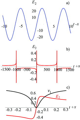
Figure 1: (Color online) Emitted in the forward direction (a) and backward reflected (b) waves for $a_{2}=25$. The electric field amplitude is divided by $\epsilon_{\alpha}$. (c) Local structure of the electric field $E_{2}$ and of the longitudinal velocity of the electron layer $v_{1}$.

Due to the double Doppler effect the wavelength of the wave reflected back by the receding layer (Fig. 1 b) is larger than the incident wavelength. In addition, the reflected wave is not sinusoidal. The minimal electric field where $\partial{E}_{2,\alpha}(x,t)/\partial x=0$ is equal to $\epsilon_{\alpha}/a_{2}$ in the limit $a_{2}\gg 1$. In this limit every each half-period the wave profile becomes singular at the point where $\partial x/\partial t_{\alpha}(x,t)=0$. In the vicinity of the singular point $t+x$ and $E_{2}$ depend on $\tau_{\alpha}$ as $t+x\approx\tau_{\alpha}-a_{2}^{2}\tau_{\alpha}^{3}/3$ and $E_{2}\approx a_{2}\tau_{\alpha}-a_{2}^{2}\tau_{\alpha}^{3}$, which gives

$$E_{2}\approx a_{2}(t+x)-\frac{2}{3}a_{2}^{2}(t+x)^{3}.$$ (36)

The electric field reaches the maximum $E_{2,m}=\sqrt{2}/3$ at $(t+x)_{m}=1/\sqrt{2}a$ with the maximum width equal to $\delta(t+x)_{m}=1/\sqrt{2}a$. As it is seen in Fig. 1 c), where we show the local structure of the electric field in the wave and the corresponding time dependence of the longitudinal velocity of the layer emitting the wave, spikes of the electric field are formed in the reflected wave when the layer stops, i.e. at $v_{x}=0$.

III.2 Frequency spectrum of the reflected EM radiation

The EM wave reflection from the electron layer accelerated by the wave is a simple model of a relativistic oscillating mirror. In the case of a linearly polarized pulse with $a_{0,2}(\tau)=a_{2}\,\sin\tau$ and $a_{0,3}(\tau)=0,$ the reflected periodic EM wave takes the form with spikes shown in Fig. 1 b). It can be represented by the Fourier series

$$E(\tau)=\sum_{n=1}^{\infty}b_{n}\sin(n\tau)$$

with Fourier coefficients $b_{n}(a)$ that vanish for even harmonic numbers $n$ and that can be expressed in terms of hypergeometric functions.

$$b_{n}=\epsilon_{\alpha}\frac{\pi a_{2}}{1+a_{2}^{2}}\times$$

$$\left[{}_{3}\tilde{F}_{2}\left(\left\{\frac{1}{2},1,1\right\},\left\{\frac{3}{2}-\frac{n}{2},\frac{1}{2}+\frac{n}{2}\right\},\frac{a_{2}^{2}}{1+a_{2}^{2}}\right)\right.$$

$$-\left.{}_{3}\tilde{F}_{2}\left(\left\{\frac{1}{2},1,1\right\},\left\{\frac{1}{2}-\frac{n}{2},\frac{3}{2}+\frac{n}{2}\right\},\frac{a_{2}^{2}}{1+a_{2}^{2}}\right)\right].$$ (37)

Here ${{}_{p}}\tilde{F}_{q}(\{a_{p}\},\{b_{q}\},z)$ is the regularized hypergeometric function equal to ${{}_{p}}{F}_{q}(\{a\},\{b\},z)/(\Gamma(b_{1})...\Gamma(b_{q}))/$. In Fig. 2 we plot the dependence of $b_{n}$ on the wave amplitude $a$ for $n=1,2,3,5,7,9$.

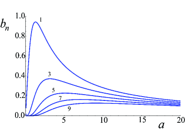
Figure 2: (Color online) Dependence of $b_{n}$ on the wave amplitude $a$ for $n=1,2,3,5,7,9$.

In the frame of reference where the layer is on average at rest the electric field spikes of the back reflected wave shown in Fig. 1 b) are formed at the moment when the mirror reaches its maximum velocity in the backward direction. The velocity of this frame is is equal to

$$v_{f}=\frac{1}{2\pi}\int_{-\pi}^{+\pi}\frac{a_{0,2}^{2}(\tau)+a_{0,3}^{2}(\tau)}{2+a_{0,2}^{2}(\tau)+a_{0,3}^{2}(\tau)}d\tau.$$ (38)

In the case of the linearly polarized wave with $a_{0,2}(\tau)=a_{0}\sin\tau$, the layer moves on average with the velocity $v_{f}=1-1/(1+a_{2}^{2}/2)^{1/2}$. The spike width and amplitude in this frame of reference changes according to the Lorentz transformation rules.

III.3 Finite radiation friction force effect

In general case, if $\epsilon_{\alpha}\neq 0$, the radiation losses lead to a finite acceleration of the layer. Now we assume that the laser radiation has the form of a Gaussian electromagnetic pulse with vector potential

$${\bf a}_{0,\perp}(x,t)={\rm exp}\left[-\frac{(t-x)^{2}}{t_{EM}^{2}}\right]$$

$$\times\left[a_{2}\cos{(t-x)}{\bf e}_{2}+a_{3}\sin{(t-x)}{\bf e}_{3}\right].$$ (39)

Numerical integration of Eq. (19) using relationships (24 – 26) yields the dependence of the longitudinal momentum $p_{1}$ on the variable $\tau_{\alpha}$ for different values of the parameters of the electromagnetic pulse and of the charged layer.

In Fig. 3 we plot the longitudinal momentum $p_{1}$ versus $\tau_{\alpha}$ for a circularly polarized electromagnetic pulse with amplitude equal to $a_{2}=a_{3}=a_{0}=5$ and length $t_{EM}=3\pi$. The parameter $\epsilon_{\alpha}$ varies from 0.03 to 2.5.

Figure 3: (Color online) Dependence of the longitudinal momentum $p_{1}$ on the variable $\tau_{\alpha}$ for different values of the parameter $\epsilon_{\alpha}$: 1. $\epsilon_{\alpha}=0.03$; 2. $\epsilon_{\alpha}=0.04$; 3. $\epsilon_{\alpha}=0.045$; 4. $\epsilon_{\alpha}=0.05$; 5. $\epsilon_{\alpha}=2.5$.

As we see, in the limit of very low $\epsilon_{\alpha}$ (curves 1 and 2) the layer momentum dependence on $\tau_{\alpha}$ follows approximately according to Eqs. (29). For larger values of $\epsilon_{\alpha}$ (curves 3 and 4) as a result of the layer interaction with a finite width electromagnetic pulse the momentum does not vanish at $\tau_{\alpha}\to+\infty$, i. e. the Lawson – Woodward theorem is not valid. When the parameter further increases (curve 5) the maximum value of the longitudinal momentum becomes lower. This fact is illustrated in Fig. 4, where the layer momentum dependence on $\epsilon_{\alpha}$ is shown for different laser pulse amplitudes.

When the interaction of the charged layer with the electromagnetic wave occurs in the regime beyond the Lawson – Woodward theorem the effects of the finite radiation friction force modify the electric charge dynamics due to its acceleration by the radiation pressure LandauLifshitzVol2 . This is seen in the curves 3,4, and 5 in Fig. 3 as a ”re-acceleration”of $p_{1}(\tau_{\alpha})$.

Figure 4: (Color online) Dependence of the longitudinal momentum $p_{1}$ on the parameter $\epsilon_{\alpha}$ for different values of the electromagnetic pulse amplitude: 1. $a_{0}=1.25$; 2. $a_{0}=2.5$; 3. $a_{0}=5$; 4. $a_{0}=7.5$.

Fig. 5 presents the dependence of the layer momentum $p_{1}$ on the electromagnetic wave amplitude for different values of the parameter $\epsilon_{\alpha}$.

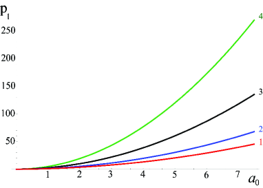
Figure 5: (Color online) Dependence of the longitudinal momentum $p_{1}$ on the electromagnetic pulse amplitude $a_{0}$ for different values of the parameter $\epsilon_{\alpha}$ : 1. $\epsilon_{\alpha}=1.25$; 2. $\epsilon_{\alpha}=2.5$; 3. $\epsilon_{\alpha}=5$; 4. $\epsilon_{\alpha}=7.5$.

The plot in Fig. 6 shows isocontours of equal value of $\gamma_{\alpha}$ in the plane $\epsilon_{\alpha},a_{0}$

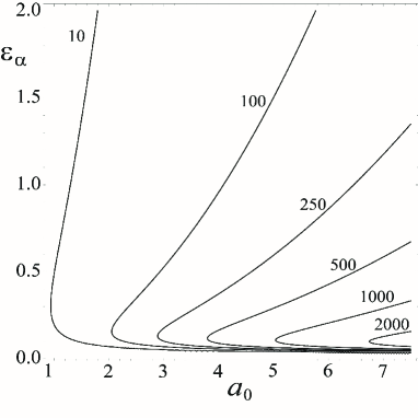
Figure 6: Isocontours of equal value of $\gamma_{\alpha}$ in the plane $\epsilon_{\alpha},a_{0}$.

As we see the maximum acceleration efficiency corresponds to the wave amplitude of the order of $1/\epsilon_{\alpha}$ .

IV Relativistic oscillating mirror

The Relativistic Oscillating Mirror (ROM) concept has been proposed in Ref. RelOscMirr as a mechanism of high order harmonic generation when an overdense plasma is irradiated by a relativistically intense laser radiation. The generation of high frequency radiation in thus interaction regime was experimentally demonstrated in Refs. Dromey_ROM . Within the framework of the ROM concept, attention is paid to the fact that under the laser field action the critical density region from which the light is reflected oscillates periodically back and forth forming in other words an oscillating mirror. Due to the Doppler effect when the wave reflects from the relativistic mirror its frequency spectrum extends into the high frequency range and the wave breaks up into short wave packets. The reflected wave frequency is upshifted to a range determined by a factor approximately equal to $4\gamma_{M}^{2}$, where $\gamma_{M}$ is the relativistic gamma factor associated with the mirror motion. A detailed discussion of the main features of the ROM theory and its experimental demonstration can be found in the review articles photon-rev1 . A thin foil made of two layers of electrons and ions irradiated by a high intensity electromagnetic wave provides a good theoretical model elucidating the basic features of the ROM concept. In this Section we assume that the ion layer is at the rest at $x_{i}=0$. When the electron layers moves with respect to the ion layer an electric field due to charge separation is generated equal to

$${\bf E}(x)=-\epsilon_{e}{\rm sgn}(x){\bf e}_{1}.$$ (40)

We consider an electromagnetic pulse whose form is given by Eq. (39), normally incident on the foil. The the amplitude and the duration of this linearly polarized short pulse are $a_{0}=25$ and $t_{EM}=5\pi$, respectively. The ion layer is assumed to be at the rest at $x=0$. In the numerical integration, in the expression for the restoring electric field $E(x)$, we replace the discontinuous function ${\rm sgn}(x)$ by ${\rm Tanh}(x/l)$ with the plasma layer thickness equal to $l=0.01$. Before the laser pulse hits the target $t\to-\infty$ the electrons are located at $x=0$ with ${\bf p}_{0}=0$.

IV.1 Opaque mirror

We take the dimensionless parameter $\epsilon_{e}$, that characterizes both the radiation losses and the electric charge separation electric field, equal to $\epsilon_{e}=50$. This choice corresponds to the limit when $a_{0}\ll\epsilon_{e}$, and thus in this case the foil is almost opaque for the incident EM radiation. The electric charge separation field is relatively strong which results in the electron layer oscillations remaining in close proximity of the ion layer. Figs. 7 and 8 illustrate the main features of the linearly polarized EM pulse interaction with the opaque foil target. As we see in Fig. 7 the electron layer oscillates at the front of the ion layer due to the combined effect of the reflected electromagnetic pulse and of the restoring force due to the ion layer: the net displacement at the end of the pulse interaction is much smaller than the oscillation amplitude. The average longitudinal momentum of the electron layer is also almost zero. The reflected and transmitted waves plotted in Fig. 8 resemble the incident EM pulse (39). The EM wave is almost completely reflected with the maximum amplitude of the reflected wave equal to 24.4. The transmitted wave calculated as the superposition of the incident wave and of the wave emitted forwards by the electron layer, which almost cancel each other, has its maximum amplitude equal to 0.6.

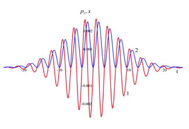
Figure 7: (Color online) Time dependence of the longitudinal electron momentum, $p_{1}(t)$, (red curve) and of the layer coordinate, $x_{1}(t)$, (blue curve) for $a_{0}=25$, $t_{EM}=5\pi$ and $\epsilon_{e}=50$.

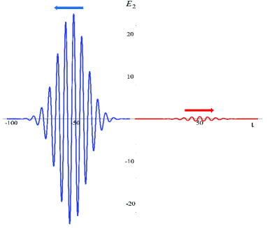
Figure 8: (Color online) Reflected, $E_{2}(t+x)$, (blue curve) and transmitted, $E_{2}(t-x)$, (red curve) waves for $a_{0}=25$, $t_{EM}=5\pi$ and $\epsilon_{e}=50$.

IV.2 Transparent mirror

The case of a transparent foil target with $a_{0}\gg\epsilon_{e}$ is shown in Figs. 9 and 10 for $a_{0}=25$ and $\epsilon_{e}=5$

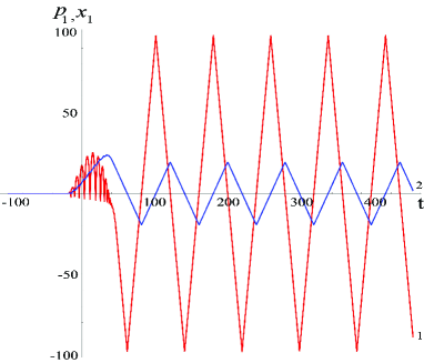
Figure 9: (Color online) Time dependence of the longitudinal electron momentum, $p_{1}(t)$, (red curve, 1) and of the layer coordinate, $x_{1}(t)$, (blue curve, 2) for $a_{0}=25$, $t_{EM}=5\pi$ and $\epsilon_{e}=5$.

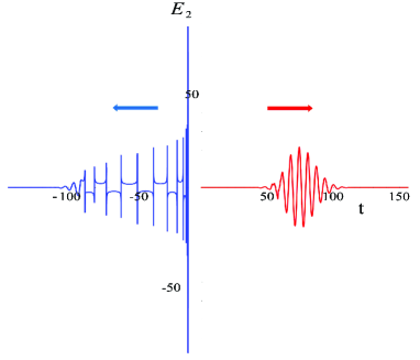
Figure 10: (Color online) Reflected, $E_{2}(t+x)$, (blue curve) and transmitted, $E_{2}(t-x)$, (red curve) waves for $a_{0}=25$, $t_{EM}=5\pi$ and $\epsilon_{e}=5$.

In this regime of the EM wave interaction with the double layer target the radiation pressure pushes the electron layer forwards. The interaction is nonadiabatic with respect to the longitudinal “sawtooth” oscillation excitation which are seen in the longitudinal electron momentum and coordinate dependence on time presented in Fig. 9. Similar oscillations have been noticed in Ref. MikhPRL . In contrast to the opaque case, the net layer displacement at the end of the interaction of the pulse with the layer is not small and provides the initial condition for the “sawtooth” oscillations that are a periodic sequence of hyperbolic motions of the electric charge in the homogeneous electric field LandauLifshitzVol2 due to the ion layer. Within an oscillation half cycle the electron layer momentum depends on time as

$$p_{1}(t)=p_{m}-\epsilon_{e}t$$ (41)

in the time interval $0<t<t_{m}$, where $t_{m}$ is the half-cycle duration equal to $2p_{m}/\epsilon_{e}$. The time dependence of the layer coordinate is given by

$$x_{1}(t)=\frac{1}{\epsilon}\left[\sqrt{1+p_{m}^{2}}-\sqrt{1+(p_{m}-\epsilon_{e}t)^{2}}\right]$$ (42)

The maximum of the electron layer momentum $p_{m}$ and the maximum of the layer displacement $x_{m}$ are related to each other as

$$p_{1,m}=\sqrt{(1+\epsilon_{e}x_{1,m})^{2}-1}.$$ (43)

In order to find $x_{1,m}$ in the limit $a_{0}\gg\epsilon_{e}$ we can use expression (33), which for the Gaussian linearly polarized EM pulse (39) yields

$$x_{1,m}=a_{0}^{2}\frac{\left[1-\exp\left(-t_{EM}^{2}/2\right)\right]\sqrt{\pi}t_{EM}}{2^{5/2}}.$$ (44)

The condition of nonadiabatic interaction is $t_{m}>t_{EM}$. The electron kinetic energy found from Eqs. (43) and (45) is given by

$$\frac{{\cal E}_{e}}{m_{e}c^{2}}=\gamma_{e}-1=\epsilon_{e}x_{1,m}\approx\sqrt{\frac{\pi}{32}}a_{0}^{2}\epsilon_{e}t_{EM},$$ (45)

which for $a_{0}^{2}\epsilon_{e}t_{EM}\gg 1$ is well above the quiver energy of an electron moving in the EM wave. The excitation of the sawtooth oscillations can be regarded as the efficient collisionless heating of the electrons. This in fact can be an underlying mechanism of the electron energization during high intensity laser radiation interaction with a thin foil target observed in the computer simulations presented in Ref. IONS-UL (see Fig. 1 (b) therein).

The transmitted and reflected waves shown in Fig. 10 have approximately of the same amplitude level because the receding relativistic mirror becomes less transparent while it is accelerated in the forward direction photon-rev3 ; MacchiPRLReflectivity ; BulanovOptimalShape . This results in a relative enhancement of the reflected wave amplitude. The spectra of the reflected and transmitted radiation contain high order harmonics. The reflected wave has the form of ultrashort spikes. The distance between them corresponds to the stretched wavelength of the incident light due to the double Doppler effect, because part of the wave interaction with the oscillating electron layer occurs under the conditions of reflection from a receding mirror. We note that the strongest spike at the rear of the reflected pulse is formed due to interaction with the sawtooth oscillations.

V Relativistic flying mirror

A method to generate high frequency radiation based on the concept of the Relativistic Flying Mirror (RFM) considers a thin plasma shell travelling close to the speed of light as a relativistic mirror. The reflected light undergoes frequency upshift, compression and intensification due to a relativistic double Doppler effect. Various schemes were described photon-rev3 ; BulanovRMP ; Bulanov2006 ; Kulagin2007 ; Kulagin2013 ; Kagami ; BrII2012 ; Lobet and experimentally demonstrated Kando2007 ; Foil3 as a proof of the feasibility of this concept.

V.1 The shape of a pulse reflected from a relativistic flying mirror

Using a double layer thin foil target as a RFM model, we consider the configuration of two counter propagating pulses. The first EM pulse driver pushes the electron layer forwards with relativistic velocity. The second pulse is relatively week and propagates in the opposite direction. As a result of its head-on collision with the RFM a portion of the photons from this pulse is back reflected. This process is accompanied by the frequency upshifting of the reflected photons and by the modulation of the reflected pulse. When the ponderomotive force of the driver EM pulse is substantially larger than the force from the electric field due to the electric charge separation, i. e. when $\epsilon_{e}\ll a_{0}$, the motion of the relativistic electron layer can be described by Eqs. (28 – 32). In the case when the electron layer is accelerated by a linearly polarized EM pulse, as analysed in Ref. photon-rev3 , the phase of the reflected part of the weaker EM wave is given by

$$\psi_{r}(u)=\omega_{s}\left(u+\frac{a_{0}^{2}}{2}u-\frac{a_{0}^{2}}{4\omega}\sin 2\omega u\right)$$ (46)

with $u=t-x$ and $\omega_{s}$ the frequency of the EM source pulse. The reflected pulse frequency given by a derivative of the phase $\psi_{r}$ with respect to time is

$$\omega_{r}(u)=\omega_{s}\left(1+a_{0}^{2}\sin^{2}\omega u\right)$$ (47)

The frequency upshifting factor $g=\omega_{r}/\omega_{s}$ depends on the longitudinal velocity of the mirror, $v_{1}=p_{1}/\gamma$ as

$$g=\frac{\gamma+p_{1}}{\gamma-p_{1}}.$$ (48)

If the source pulse frequency is equal to the driver pulse frequency, $\omega_{s}=\omega=\omega_{0}$, the reflected pulse frequency, $\omega_{r}=\omega_{0}(1+a_{0}^{2}\sin^{2}\omega_{0}u)$, changes from $\omega_{0}$ to $\omega_{0}(1+a_{0}^{2})$. The wave amplitude is modulated accordingly. The reflected radiation consists of a sequence of short high frequency pulses.

Fig. 11 shows the results of the numerical integration of Eqs. (13 – 15). The Gaussian EM pulse driver is linearly polarized with $a_{2}=15,\qquad a_{3}=0$ and $t_{EM,d}=5\pi$. The source EM pulse is linearly polarized in the perpendicular plane, with $a_{2}=0,\qquad a_{3}=1$ and $t_{EM,s}=150\pi$.

In Fig. 11 a) we plot the time dependence of the longitudinal momentum, $p_{1}(t)$, of the electron layer (red curve), of the layer coordinate, $x_{1}(t)$, (blue curve) and of the factor $g(t)$ (black curve) for the driver EM pulse with $a_{2}=15$, $t_{EM,d}=5\pi$ and $\epsilon_{e}=0.1$.

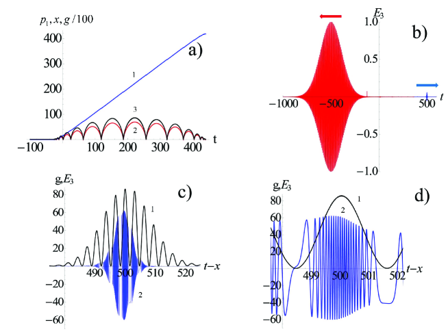
Figure 11: (Color online) a) Time dependence of the longitudinal electron layer momentum, $p_{1}(t)$, (red curve), of the layer coordinate, $x_{1}(t)$, (blue curve) and of the factor $g(t)$ (black curve) for the driver EM pulse with $a_{2}=15$, $t_{EM,d}=5\pi$ and $\epsilon_{e}=0.1$. Counterpropagating source pulse: b) Reflected, $E_{3}(t-x)$, (blue curve) and transmitted, $E_{3}(t+x)$, (red curve) waves for $a_{3}=1$, $t_{EM,s}=150\pi$ and $\epsilon_{e}=0.1$. c) Reflected pulse (blue curve) and frequency upshifting factor $g(t)$ (black curve). d) Close up of the reflected pulse (blue curve) and frequency upshifting factor $g(t)$ (black curve).

The electron layer, while oscillating back and forth, moves on average forwards with a relativistic velocity. The frequency upshifting factor $g$ oscillates synchronously with the layer momentum $p_{1}$. According to expressions (29 – 32) and (48) the factor $g$ and the layer longitudinal momentum are related in the limit $a_{0}\gg\epsilon_{e}$ as $g=1+2p_{1}$, i.e. the factor $g$ scales with the layer energy as $g=\sim 2\gamma_{e}$. For the chosen EM pulse driver amplitude equal to $15$ the maximum value of the factor $g$ is 226.

In Fig. 12 we present the frequency spectrum of the driver and source pulses. Fig. 12 a) shows the dependence of the absolute value of the Fourier transform of the $E_{2}$ component of the electric field, corresponding to the incident and transmitted electromagnetic of the driver pulse. In Fig. 12 b) we plot the dependence of the absolute value of the Fourier transform of the $E_{3}$ component of the electric field, which corresponds to the incident and reflected electromagnetic of the source pulse. The spectrum of the reflected radiation is enriched by the high order harmonics. It has a form of the plateau, which extends to the value of the order of $\omega_{\max}\approx\omega_{0}g$

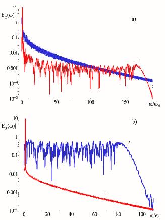
Figure 12: (Color online) The frequency spectrum of the driver and source pulses. a) The dependence of the absolute value of the Fourier transform of the $E_{2}$ component of the electric field, corresponding to the incident and transmitted electromagnetic of the driver pulse. b) The dependence of the absolute value of the Fourier transform of the $E_{3}$ component of the electric field, which corresponds to the incident and reflected electromagnetic of the source pulse.

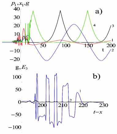
Figure 13: (Color online) Counterpropagating driver and source pulses of equal amplitude and duration. a) Time dependence of the longitudinal electron layer momentum, $p_{1}(t)$, (red curve), the layer coordinate, $x_{1}(t)$, (blue curve), the factors $g_{+}(t)$ (black curve) and $g_{-}(t)$ (green curve), for the driver EM pulse with $a_{2}=15$, $a_{3}=15$, $t_{EM,d}=t_{EM,s}=3\pi$ and $\epsilon_{e}=0.1$. b) Reflected pulse $E_{3}(t-x)$(blue curve) and frequency upshifting factor $g_{+}(t)$ (black curve).

The reflected EM pulse as seen in Fig. 11 b) is approximately shorter by a factor $g=226$ than the source pulse incident on the foil. Fig. 11 c) shows that the reflected wave breaks up into a train of high frequency pulses, which are frequency modulated (see Fig. 11 d)), i.e. in general the frequency upshifting and shortening of the reflected pulse is accompanied by the generation of high order harmonics.

The amplitude of the reflected EM pulse is proportional to the amplitude of the incident radiation, $a_{s}$, times the factor $g$ and times the reflection coefficient $\rho$. The reflection coefficient can be found as in Refs. Foil1 ; photon-rev3 ; MacchiPRLReflectivity ; BulanovOptimalShape ; BrII2012 . In the frame of reference co-moving with the electron layer where the longitudinal momentum component vanishes, $p_{1}=0$, the equation for the electric field, ${\bf E}={\bf E}_{0}+{\bf E}_{e,l}$, according to Eqs. (5) and (10) can be written in the form

$${\bf E}^{\prime}={\bf E}^{\prime}_{0}+\frac{2\pi enl}{c}{\bf v}^{\prime}_{\perp},$$ (49)

where a prime denotes the electric field and the electron velocity in the co-moving frame of reference and ${\bf v}^{\prime}_{\perp}=v^{\prime}_{2}{\bf e}_{2}+v^{\prime}_{3}{\bf e}_{3}$. Here we use dimensional variables, i.e. $2\pi enl$ instead $\epsilon_{e}$, in order to clearly show that the areal charge density, $enl$, is Lorentz invariant while the electric field and the electron velocity are not invariant. In the head-on collision configuration of the EM pulse interaction with the electron layer when $v_{1}<0$ the electric field in the boosted frame is larger than that in the laboratory frame of reference by a factor of $\sqrt{(1+|v_{1}|)/(1-|v_{1}|)}\approx 2\gamma$.

Since in any frame of reference the electron velocity cannot exceed the speed of light in vacuum, there are two limiting cases depending on the value of $E^{\prime}_{0}/2\pi enl\approx 4\gamma^{2}a_{s}/\epsilon_{e}$. In the case of a weak EM wave, when this ratio is much smaller than unity, from Eq. (49) it follows that the amplitudes of the incident, $E^{\prime}$, and reflected, $2\pi enl{\bf v}^{\prime}_{\perp}/c$, waves are almost equal to each other, i.e. the reflection coefficient is of the order of unity. In the opposite limit, when $E^{\prime}_{0}/2\pi enl\gg 1$, the amplitude of the reflected EM wave in the boosted frame of reference is of the order of $2\pi enl$. This yields a constraint on the upper limit of the EM radiation intensity measured in the laboratory frame of reference, when the wave is reflected by a thin electron layer of areal density $nl$ moving with relativistic gamma-factor $\gamma$, as in the above considered case or in the flying mirror configuration discussed in Ref. Kulagin2007 : $I_{r}\leq 16\pi c(enl)^{2}\gamma^{2}$. For example, for an 10${}^{-2}\mu$m, $n=10^{23}{\rm cm}^{-3}$ electron layer moving with the gamma-factor equal to 10² this yields $I_{r}\approx 5\times 10^{25}$W/cm².

In Fig. 13 we illustrate the regime when two EM pulses with equal amplitudes and perpendicular polarizations interact with a thin foil target. The amplitudes of the driver and source pulses are equal to $a_{2}=15$, $a_{3}=15$, $t_{EM,s}=t_{EM,d}=3\pi$ and $\epsilon_{e}=0.1$. In Fig. 13 a), we plot the time dependence of the electron layer coordinate $x(t)$, momentum component $p_{1}(t)$ and of the frequency upshifting factors $g_{+}$ and $g_{-}$, for the waves reflected to the right and to the left hand side directions, respectively. As seen, during the interaction of the two EM pulses colliding head-on the electron layer undergoes irregular jigglings. The frequency upshifting factors are not as large as in the previous case presented in Fig. 11. The reflected EM wave shown in Fig.13 b) has a non-sinusoidal form and is much less regular than in the case of a source pulse with a finite but not too large amplitude described by Figs. 13 c) and d).

V.2 Head on interaction of an EM pulse with an electron layer in the regime of sawtooth oscillations

As noticed above (48), if the electron layer is driven by an electromagnetic wave with amplitude $a_{0}$ the frequency upshifting factor for a counterpropagating pulse cannot exceed the value $g\leq(1+a_{0}^{2})$. However, the $g$ factor can be substantially enhanced by imposing a delay between the driver and the source pulses in a such a way that the counterpropagating source pulse gets reflected by the electron layer in the phase when the layer undergoes “sawtooth” oscillations. According to Eq. (45) the mirror Lorentz factor scales as $a_{0}^{2}\epsilon_{e}t_{EM}$, i. e. the the frequency upshifting factor may be of the order of $\approx 4a_{0}^{4}\epsilon_{e}^{2}t_{EM}^{2}$. In other words the longitudinal velocity of the electron layer during the phase of “sawtooth” oscillations, i.e. after the end of the driver EM pulse, is substantially larger than the velocity of the oscillations driven by the ponderomotive force as clearly seen in Fig. 9. By choosing the delay time between the driver and the counter propagating source pulse in a such way that the source pulse collides with the electron layer at the “sawtooth” oscillation phase, we can provide conditions for a much higher frequency upshifting and intensification of the back-reflected radiation in the regime as shown in Fig. 14.

Figure 14: (Color online) a)Time dependence of the longitudinal electron layer momentum, $p_{1}(t)$, (red curve), of the layer coordinate, $x_{1}(t)$, (blue curve) and of the factor $g(t)$ divided by 100 (black curve) for a driver EM pulse with $a_{2}=25$, $t_{EM,d}=5\pi$ and $\epsilon_{e}=1$. b) Reflected pulse $E_{3}(t-x)$(blue curve). c) Incident source pulse $E_{3}(t+x)$(green curve)

The source pulse is polarized in the plane perpendicular to the driver pulse polarization plane. Its amplitude is equal to 0.001 and its width is $t_{EM,s}=40\pi$. The delay time between the driver and source pulses is $230\pi$. In Fig. 14 a) the time dependence of the longitudinal electron layer momentum, $p_{1}(t)$, (red curve), the layer coordinate, $x_{1}(t)$, (blue curve) and the divided by 100 factor $g(t)$ (black curve) for the driver EM pulse with $a_{2}=25$, $t_{EM,d}=5\pi$ and $\epsilon_{e}=1$ are shown. The frequency upshifting factor reaches its maximum $\approx 1.2\times 10^{5}$ at $t=725$. The reflected source pulse shown in Fig. 14 b) has amplitude $E_{3}=0.4$ approximately $4\times 10^{3}$ times larger than that of the incident wave (see Fig. 14 c)). Its width and wavelength are shortened by a factor $g$. The form of the reflected EM pulse resembles that of the frequency upshifting factor $g(t)$ (see Figs. 14) a) and b)).

VI Ion acceleration

In Ref. IONS the radiation pressure exerted by an ultraintense electromagnetic pulse on a quasineutral plasma foil has been proposed as a very efficient acceleration mechanism capable of providing ultrarelativistic ion beams. In this radiation pressure dominant acceleration (RPDA) regime, the ions move forward under the push of the pulse pressure with almost the same velocity as the electrons. A fundamental feature of this acceleration process is its high efficiency, as the ion energy per nucleon turns out to be proportional in the ultrarelativistic limit to the electromagnetic pulse energy.

Recently the RPDA regime of laser ion acceleration has attracted great attention e.g., see review articles ion-rev . In Ref. RT-PB the stability of the accelerated foil has been analyzed. A foil accelerated to relativistic energies by a laser pulse can also act as a relativistic flying mirror for frequency upshift and intensification of a reflected counterpropagating light beam kagami . An indication of the effect of the radiation pressure on bulk target ions is obtained in experimental studies of thin solid targets irradiated by ultraintense laser pulses SKAR .

Below we consider a double layer (ion and electron) thin foil target irradiated by the EM radiation. For the sake of simplicity we assume that the electron layer motion is described by Eqs. (13 – 15). In the ion layer equations of motion we neglect its interaction with the EM wave retaining only the electrostatic force due to the electric field produced by the electron layer. The electrostatic approximation for the ion layer motion can be used provided the parameter $eE/m_{i}\omega c$ is small, i.e., in the case of a one micron wavelength laser, for a light intensity below $\approx 10^{24}$W/cm². At this limit the classical electrodynamics paradigm must be changed and quantum effects must be included QEDint .

The results of the numerical integration of the equations of motion of the electron and ion layers irradiated by a strong EM wave are shown in Fig. 15. Figure 15 a) presents typical regimes of ion acceleration for a linearly polarized electromagnetic pulse with amplitude $a=10$ and duration $t_{EM}=5\pi$ interacting with a foil with $\epsilon_{e}=1.5$. At the initial stage $-25<t<25$ the time dependence of the ion and electron coordinates corresponds to a strong charge separation. As seen in Fig. 15 a), the electron layer pushed by the radiation pressure of the EM wave pulls the ion layer. Then both layers move forwards with the same average velocity and with the electron layer moving back forth around the ion layer performing sawtooth oscillations. This phenomenon can explain the efficient electron heating during the RPD ion acceleration observed in the PIC simulations presented in Ref. IONS-UL . In addition these oscillations cause oscillations of the ion energy $\gamma_{i}-1$ around its average value.

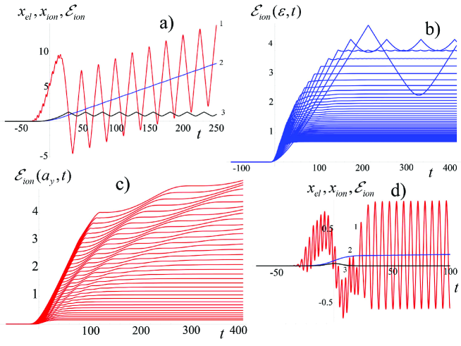
Figure 15: (Color online) Ion acceleration by the radiation pressure. a) Time dependence of the the electron (red curve) and ion (blue curve) layer coordinates and of the ion energy $m_{i}c^{2}(\gamma_{i}-1)$ (black) for an EM pulse with $a_{2}=10$, $t_{EM}=5\pi$ and $\epsilon_{e}=1.5$. b) Normalized ion energy $\gamma_{i}-1$ v.s. time for $a_{2}=400$ and the parameter $\epsilon_{e}$ varying from 45 to 250 from bottom to top with the step equal to 5. c) Normalized ion energy $\gamma_{i}-1$ v.s. time for $\epsilon_{e}=45$ and the EM pulse amplitude $a_{2}$ varying from bottom to top from 100 to 450 with the step equal to 10. d) Time dependence of the the electron (red curve) and ion (blue curve) layer coordinates and of the ion energy $m_{i}c^{2}(\gamma_{i}-1)$ (black) for the case without radiation friction.

The parametric dependence on the EM pulse amplitude and on the target surface density of the energy of the accelerated ions is illustrated in Figs. 15 b) and c). The dependence on time of the ion energy for different values of the EM pulse amplitude and varying parameter $\epsilon_{e}$ is not monotonic as seen in Figs. 15 b) and c) and can be explained by the sawtooth oscillations of the electron and ion layers. A finite value of the parameter $\epsilon_{e}$ provides an efficient coupling between the EM pulse and the electron-ion foil target. In the case without radiation friction shown in Fig. 15 d) the ion acceleration is less efficient.

VII Conclusions, Discussions, Main Results

The theory of the interaction of relativistically strong electromagnetic fields with foil targets used in the present paper is based on the thin layer model of the one-dimensional electrodynamics of charged particles. It describes the 1D motion of electric charges in the self-consistent electromagnetic field incorporating the charge self-action or, in other words, the effect of the radiation friction force.

Within this framework, the generation of high order harmonics in the relativistic regime occurs through the electromagnetic wave reflection, or collective backward scattering also called nonlinear collective Thomson scattering, at the electron layer driven by the electromagnetic wave. The back reflected radiation takes the form of a train of ultrashort single-cycle electromagnetic pulses that are formed at the moment of maximal negative velocity of the layer.

The radiation scattered by the thin foil target in the backward and that scattered in the forward direction have different frequency spectra.

In the nonadiabatic regime of interaction with the ion-electron layer target a short electromagnetic pulse excites relatively low frequency sawtooth oscillations with amplitude substantially larger than the amplitude of the oscillations of the electron layer driven by the electromagnetic pulse. These sawtooth oscillations provide a mechanism of collective electron heating. They also generate extremely short spikes in the reflected EM wave.

In the configuration when two electromagnetic beams irradiate the thin foil target the electron layer driven by strong enough electromagnetic wave plays the role of a relativistic flying mirror for the second pulse. The electromagnetic radiation reflected from the relativistic mirror counterpropagating is intensified and its frequency is substantially increased. The reflected radiation takes the form of a sequence of the high frequency short bunches of electromagnetic radiation.

Since the longitudinal velocity of the electron layer during the phase of the “sawtooth” oscillations is substantially larger than the velocity of the oscillations driven within the electromagnetic pulse driver, by choosing the delay time between the driver and the counter propagating source pulse in a such way that the source pulse collides with the electron layer at the “sawtooth” oscillation phase, we can provide conditions for high frequency upshifting and intensification of the back-reflected radiation.

Under the radiation pressure of the electromagnetic wave the electron layer becomes separated from the ion layer that moves in the electric field due the charge separation. As a result, while the electron layer undergoes back and forth sawtooth oscillations around the ion layer, on average both layers move together. The ion acceleration rate grows higher with higher amplitude of the incident electromagnetic wave. It also depends on the radiation friction which is responsible for the coupling of the electromagnetic field with the electron layer because it provides the wave back scattering and thus the momentum transfer from the electromagnetic field to the charge particles. If the radiation friction force effects are not taken into account the ion acceleration rate is substantially lower for the same electromagnetic pulse amplitude.

References

- (1) M. Borghesi, J. Fuchs, S. V. Bulanov, A. J. MacKinnon, P. K. Patel, and M. Roth, Fus. Sci. Techn. 49, 412 (2006); H. Daido, M. Nishiuchi, and A. S. Pirozhkov, Rep. Prog. Phys. 75, 056401 (2012); A. Macchi, M. Borghesi, and M. Passoni, Rev. Mod. Phys. 85, 751 (2013).
- (2) E. Esarey, C. B. Schroeder, and W. P. Leemans, Rev. Mod. Phys. 81, 1229 (2009).
- (3) U. Teubner and P. Gibbon, Rev. Mod. Phys. 81, 445 (2009); F. Krausz and M. Ivanov, Rev. Mod. Phys. 81, 163 (2009).
- (4) S. Corde, K. Ta Phuoc, G. Lambert, R. Fitour, V. Malka, A. Rousse, A. Beck, E. Lefebvre, Rev. Mod. Phys. 85, 1 (2013).
- (5) S. V. Bulanov, T. Zh. Esirkepov, A. S. Pirozhkov, and N. N. Rosanov, Physics Uspekhi 56, 429 (2013).
- (6) G. Mourou, T. Tajima, and S. V. Bulanov, Rev. Mod. Phys. 78, 309 (2006).
- (7) M. Marklund and P. Shukla, Rev. Mod. Phys. 78, 591 (2006); A. Di Piazza, C. Muller, K. Z. Hatsagortsyan, and C. H. Keitel, Rev. Mod. Phys. 84, 1177 (2012).
- (8) B. A. Remington, D. Arnett, R. P. Drake, and H. Takabe, Science 284, 1488 (1999); B. Remington, R. P. Drake, and D. Ryutov, Rev. Mod. Phys. 78, 755 (2006); S. V. Bulanov, T. Zh. Esirkepov, D. Habs, F. Pegoraro, and T. Tajima, Eur. Phys. J. D 55, 483 (2009).
- (9) V. A. Vshivkov, N. M. Naumova, F. Pegoraro, S. V. Bulanov, Phys. Plasmas 5, 2727 (1998).
- (10) T. Esirkepov, M. Borghesi, S. V. Bulanov, G. Mourou, and T. Tajima, Phys. Rev. Lett. 92, 175003 (2004).
- (11) S. V. Bulanov, E. Yu. Echkina, T. Zh. Esirkepov, I. N. Inovenkov, M. Kando, F. Pegoraro, and G. Korn, Phys. Rev. Lett. 104, 135003 (2010); S. V. Bulanov, E. Yu. Echkina, T. Zh. Esirkepov, I. N. Inovenkov, M. Kando, F. Pegoraro, and G. Korn, Phys. Plasmas 17, 063102 (2010).
- (12) H. K. Avetissian, A. K. Avetissian, G. F. Mkrtchian, and Kh.V. Sedrakian, Phys. Rev. STAB 14, 101301 (2011).
- (13) A. Macchi, S. Veghini, and F. Pegoraro, Phys. Rev. Lett. 103, 085003 (2009); S. V. Bulanov, T. Zh. Esirkepov, Y. Hayashi, M. Kando, H. Kiriyama, J. K. Koga, K. Kondo, H. Kotaki, A. S. Pirozhkov, S. S. Bulanov, A. G. Zhidkov, P. Chen, D. Neely, Y. Kato, N. B. Narozhny, and G. Korn, Nucl. Instr. Meth. Phys. Res. A 653, 153 (2011).
- (14) S. S. Bulanov, C. B. Schroeder, E. Esarey, and W. P. Leemans, Phys. Plasmas 19, 093112 (2012).
- (15) S. V. Bulanov, N. M. Naumova, and F. Pegoraro, Phys. Plasmas 1, 745 (1994).
- (16) A. S. Pirozhkov, S. V. Bulanov, T. Zh. Esirkepov, M. Mori, A. Sagisaka and H. Daido, Phys. Lett. A 349, 256 (2006); A. S. Pirozhkov, S. V. Bulanov, T. Zh. Esirkepov, M. Mori, A. Sagisaka and H. Daido, Phys. Plasmas 13, 013107 (2006).
- (17) J. M. Mikhailova, M. V. Fedorov, N. Karpowicz, P. Gibbon, V. T. Platonenko, A. M. Zheltikov, and F. Krausz, Phys. Rev. Lett. 109, 245005 (2012).
- (18) B. Dromey, M. Zepf, A. Gopal, K. Lancaster, M. S. Wei, K. Krushelnick, M. Tatarakis, N. Vakakis, S. Moustaizis, R. Kodama, M. Tampo, C. Stoeckl, R. Clarke, H. Habara, D. Neely, S. Karsch, and P. Norreys, Nat. Phys. 2, 456 (2006); B. Dromey, S. Kar, C. Bellei, D. C. Carroll, R. J. Clarke, J. S. Green, S. Kneip, K. Markey, S. R. Nagel, P. T. Simpson, L. Willingale, P. McKenna, D. Neely, Z. Najmudin, K. Krushelnick, P. A. Norreys, and M. Zepf, Phys. Rev. Lett. 99, 085001 (2007); B. Dromey, D. Adams, R. H rlein, Y. Nomura, S. G. Rykovanov, D. C. Carroll, P. S. Foster, S. Kar, K. Markey, P. McKenna, D. Neely, M. Geissler, G. D. Tsakiris, and M. Zepf, Nat. Phys. 5, 146 (2009); B. Dromey, S. Rykovanov, M. Yeung, R. H rlein, D. Jung, D. C. Gautier, T. Dzelzainis, D. Kiefer, S. Palaniyppan, R. Shah, J. Schreiber, H. Ruhl, J. C. Fernandez, C. L. S. Lewis, M. Zepf, and B. M. Hegelich, Nat. Phys. 8, 804 (2012).
- (19) F. Dollar, P. Cummings, V. Chvykov, L. Willingale, M. Vargas, V. Yanovsky, C. Zulick, A. Maksimchuk, A. G. R. Thomas, and K. Krushelnick, Phys. Rev. Lett. 110, 175002 (2013).
- (20) S. V. Bulanov, T. Zh. Esirkepov, and T. Tajima, Phys. Rev. Lett. 91, 085001 (2003).
- (21) S. S. Bulanov, T. Zh. Esirkepov, F. F. Kamenets, and F. Pegoraro, Phys. Rev. E 73, 036408 (2006); S. S. Bulanov, A. Maximchuk, C. B. Schroeder, A. G. Zhidkov, E. Esarey, and W. P. Leemans, Phys. Plasmas 19, 020702 (2012).
- (22) V. V. Kulagin, V. A. Cherepenin, and H. Suk, Appl. Phys. Lett. 85, 3322 (2004); V. V. Kulagin, V. A. Cherepenin, M. S. Hur, and H. Suk, Phys. Plasmas 14, 113101 (2007); D. Habs, M. Hegelich, J. Schreiber, M. Gross, A. Henig, D. Kiefer, and D. Jung, Appl. Phys.B 93, 349 (2008); H.-C. Wu, J. Meyer-ter-Vehn, J. Fernandez, B. M. Hegelich, Phys. Rev. Lett. 104, 234801 (2010); S. S. Bulanov, A. Maksimchuk, K. Krushelnick, K. I. Popov, V. Y. Bychenkov, and W. Rozmus, Phys. Lett. A 374, 476 (2010); M. Wen et al., Appl. Phys. Lett. 101, 021102 (2012); H.-C. Wu and J. Meyer-ter-Vehn, Nat. Photonics 6, 304 (2012); J. K. Koga, S. V. Bulanov, T. Zh. Esirkepov, A. S. Pirozhkov, and M. Kando, Phys. Rev. E 86, 053823 (2012).
- (23) V. V. Kulagin, V. N. Kornienko, V. A. Cherepenin, H. Suk, Quantum Electronics 43, 443 (2013).
- (24) M. Kando, Y. Fukuda, A. S. Pirozhkov, J. Ma, I. Daito, L.-M. Chen, T. Zh. Esirkepov, K. Ogura, T. Homma, Y. Hayashi, H. Kotaki, A. Sagisaka, M. Mori, J. K. Koga, H. Daido, S. V. Bulanov, T. Kimura, Y. Kato, and T. Tajima, Phys. Rev. Lett. 99, 135001 (2007); A. S. Pirozhkov, J. Ma, M. Kando, T. Zh. Esirkepov, Y. Fukuda, L.-M. Chen, I. Daito, K. Ogura, T. Homma, Y. Hayashi, H. Kotaki, A. Sagisaka, M. Mori, J. K. Koga, T. Kawachi, H. Daido, S. V. Bulanov, T. Kimura, Y. Kato, and T. Tajima, Plasma Phys. 14, 123106 (2007); M. Kando, A. S. Pirozhkov, K. Kawase, T. Zh. Esirkepov, Y. Fukuda, H. Kiriyama, H. Okada, I. Daito, T. Kameshima, Y. Hayashi, H. Kotaki, M. Mori, J. K. Koga, H. Daido, A. Ya. Faenov, T. Pikuz, J. Ma, L.-M. Chen, E. N. Ragozin, T. Kawachi, Y. Kato, T. Tajima, and S. V. Bulanov, Phys. Rev. Lett. 103, 235003 (2009).
- (25) T. Zh. Esirkepov, S. V. Bulanov, M. Kando, A. S. Pirozhkov, and A. G. Zhidkov, Phys. Rev. Lett. 103, 025002 (2009).
- (26) A. V. Panchenko, T. Zh. Esirkepov, A. S. Pirozhkov, M. Kando, F. F. Kamenets, and S. V. Bulanov, Phys. Rev. E 78, 056402 (2008). S. V. Bulanov, T. Zh. Esirkepov, M. Kando, J. K. Koga, A. S. Pirozhkov, T. Nakamura, S. S. Bulanov, C. B. Schroeder, E. Esarey, F. Califano, and F. Pegoraro, Phys. Plasmas 19, 113102(2012); Phys. Plasmas 19, 113103 (2012).
- (27) S. V. Bulanov, T. Zh. Esirkepov, N. M. Naumova, F. Pegoraro, I. V. Pogorelsky, A. M. Pukhov, IEEE Trans. Plasma Sci. 24, 393 (1996).
- (28) S. A. Reed, T. Matsuoka, S. S. Bulanov, M. Tampo, V. Chvykov, G. Kalintchenko, P. Rousseau, V. Yanovsky, R. Kodama, D. W. Litzenberg, K. Krushelnick, and A. Maksimchuk, Appl. Phys. Lett. 94, 201117 (2009).
- (29) D. Kiefer, M. Yeung, T. Dzelzainis, P. S. Foster, S. G. Rykovanov, C. LS. Lewis, R.S. Marjoribanks, H. Ruhl, D. Habs, J. Schreiber, M. Zepf, and B. Dromey, Nat. Comm. 4, 1763 (2013).
- (30) S. Palaniyappan, B. M. Hegelich, H.-C. Wu, D. Jung, D. C. Gautier, L. Yin, B. J. Albright, R. P. Johnson, T. Shimada, S. Letzring, D. T. Offermann, J. Ren, C. Huang, R. Horlein, B. Dromey, J. C. Fernandez, and R. C. Shah, Nature Phys. 8, 763 (2012).
- (31) M. S. Hur, Y.-K. Kim, V. V. Kulagin, I. Nam, and H. Suk, Phys. Plasmas 19, 073114 (2012).
- (32) S. V. Bulanov, Radiophys. Quantum Electronics 18, 1511 (1975).
- (33) V. I. Bratman and S. V. Samsonov, Phys. Lett. A 206, 377 (1995).
- (34) S. V. Bulanov, T. Zh. Esirkepov, M. Kando, J. Koga, and S. S. Bulanov, Phys. Rev E 84, 056605 (2011).
- (35) R. P. Feynman, R. P. Leiton, and M. Sands, The Feynman Lectures on Physics, Vol. 2 (Addison-Wesley, Reading, MA, 1966) Section 18-4.
- (36) L. D. Landau and E. M. Lifshitz, The Classical Theory of Fields (Pergamon, Oxford, 1975).
- (37) A. Bourdier, Phys. Fluids 26, 1804 (1983).
- (38) P. Gibbon and A. R. Bell, Phys. Rev. Lett. 68, 1535 (1992).
- (39) J. Dawson, Phys. Fluids 5, 445 (1962).
- (40) A. Einstein, Ann. Phys. (Leipzig) 17, 891 (1905).
- (41) R. Lichters, J. Meyer-ter-Vehn, and A. M. Pukhov, Phys. Plasmas 3, 3425 (1996).
- (42) F. V. Hartemann, High-Field Electrodynamics (CRC Press, Boca Raton, FL, 2002).
- (43) L. D. Landau and E. M. Lifshitz, The Classical Theory of Field, (Pergamon, Oxford, 1975).
- (44) J. D. Lawson, IEEE Trans. Nucl. Sci. NS-26, 4217 (1979).
- (45) P. M. Woodward, J. IEEE 93 Part III A, 1554 (1947).
- (46) M. Lobet, M. Kando, J. K. Koga, T. Zh. Esirkepov, T. Nakamura, A. S. Pirozhkov, and S. V. Bulanov, Phys. Lett. A 377, 1114 (2013).
- (47) F. Pegoraro and S. V. Bulanov, Phys. Rev. Lett. 99, 065002 (2007).
- (48) T. Zh. Esirkepov, S. V. Bulanov, M. Kando, A. S. Pirozhkov, A. G. Zhidkov, Phys. Rev. Lett. 103, 025002 (2009).
- (49) S. Kar, M. Borghesi, S.V. Bulanov, A. Macchi, M. H. Key, T. V. Liseykina, A. J. Mackinnon, P. K. Patel, L. Romagnani, A. Schiavi, and O. Willi, Phys. Rev. Lett. 100, 225004 (2008); S. Kar, K. F. Kakolee, B. Qiao, A. Macchi, M. Cerchez, D. Doria, M. Geissler, P. McKenna, D. Neely, J. Osterholz, R. Prasad, K. Quinn, B. Ramakrishna, G. Sarri, O. Willi, X. Y. Yuan, M. Zepf, and M. Borghesi, Phys. Rev. Lett. 109, 185006 (2012); F. Dollar, C. Zulick, A. G. R. Thomas, V. Chvykov, J. Davis, G. Kalinchenko, T. Matsuoka, C. McGuffey, G. M. Petrov, L. Willingale, V. Yanovsky, A. Maksimchuk, and K. Krushelnick, Phys. Rev. Lett. 108, 175005 (2012); I. J. Kim, K. H. Pae, C. M. Kim, H. T. Kim, J. H. Sung, S. K. Lee, T. J. Yu, I. W. Choi, C.-L. Lee, C. H. Nam, P. V. Nickles, T. M. Jeong, J. Lee, Phys. Rev. Lett. 111, 165003 (2013).
- (50) C. P. Ridgers, C. S. Brady, R. Duclous, J. G. Kirk, K. Bennett, T. D. Arber, A. P. L. Robinson, A. R. Bell, Phys. Rev. Lett. 108, 165006 (2012); A. G. R. Thomas, C. P. Ridgers, S. S. Bulanov, B. J. Griffin, and S. P. D. Mangles, Phys. Rev. X 2, 041004 (2012); S. V. Bulanov, T. Zh. Esirkepov, M. Kando, J. K. Koga, T. Nakamura, S. S. Bulanov, A. G. Zhidkov, Y. Kato, G. Korn, Proceed. SPIE-2013 Int. Conf., SPIE Optics + Optoelectronics, pp. 878015-878015-15 (2013); S. S. Bulanov, C. B. Schroeder, E. Esarey, W. P. Leemans, Physical Review A 87, 062110 (2013).