The SWELLS Survey. VI. hierarchical inference of the initial mass functions of bulges and discs

Abstract

The long-standing assumption that the stellar initial mass function (IMF) is universal has recently been challenged by a number of observations. Several studies have shown that a “heavy” IMF (e.g., with a Salpeter-like abundance of low mass stars and thus normalisation) is preferred for massive early-type galaxies, while this IMF is inconsistent with the properties of less massive, later-type galaxies. These discoveries motivate the hypothesis that the IMF may vary (possibly very slightly) across galaxies and across components of individual galaxies (e.g. bulges vs discs). In this paper we use a sample of 19 late-type strong gravitational lenses from the SWELLS survey to investigate the IMFs of the bulges and discs in late-type galaxies. We perform a joint analysis of the galaxies’ total masses (constrained by strong gravitational lensing) and stellar masses (constrained by optical and near-infrared colors in the context of a stellar population synthesis [SPS] model, up to an IMF normalisation parameter). Using minimal assumptions apart from the physical constraint that the total stellar mass $m^{*}$ within any aperture must be less than the total mass $m_{\rm tot}$ within the aperture, we find that the bulges of the galaxies cannot have IMFs heavier (i.e. implying high mass per unit luminosity) than Salpeter, while the disc IMFs are not well constrained by this data set. We also discuss the necessity for hierarchical modelling when combining incomplete information about multiple astronomical objects. This modelling approach allows us to place upper limits on the size of any departures from universality. More data, including spatially resolved kinematics (as in paper V) and stellar population diagnostics over a range of bulge and disc masses, are needed to robustly quantify how the IMF varies within galaxies.

1 Introduction

The stellar initial mass function is a quantity of great interest for a number of areas in astrophysics, ranging from the understanding of the microphysics of star formation to the demographics of stars and galaxies in the Universe. Owing to its fundamental importance, it is not surprising that substantial effort is being devoted to measuring it from astronomical observations. In the Milky Way the IMF can be inferred from resolved stellar populations although selection effects and dynamical and stellar evolution modelling are significant sources of uncertainty (see Bastian, Covey, & Meyer, 2010, for a recent review). Outside our Galaxy one has to rely on less direct probes, such as spectral features in integrated stellar populations (e.g. van Dokkum & Conroy, 2010; Conroy & van Dokkum, 2012; Spiniello et al., 2012; La Barbera et al., 2013), gravitational lensing (e.g. Treu et al., 2010; Auger et al., 2010b), and stellar kinematics (e.g. Cappellari et al., 2012; Dutton, Mendel, & Simard, 2012).

An important indirect way to characterise the IMF in distant galaxies consists of measuring the total gravitational mass (e.g., from dynamics, gravitational lensing, X-ray temperature profiles, or some combination of these) and relating this total mass to the stellar mass by using some prescription to account for the non-baryonic dark matter mass. By comparing this gravitationally-measured stellar mass with the stellar mass obtained from SPS models constrained by the observed colours of the galaxies, one can infer the normalisation of the IMF (e.g. Bell & de Jong, 2001). In the past few years, these methods have provided evidence against a universal IMF. Early-type galaxies much more massive than the Milky Way seem to prefer “heavy” IMFs, where we use this term to refer to IMFs that yield mass to light ratios comparable to or larger than those obtained for a Salpeter IMF (e.g. Barnabè et al., 2013; Tortora, Romanowsky, & Napolitano, 2013; Cappellari et al., 2012; Sonnenfeld et al., 2012; Auger et al., 2010a; Treu et al., 2010). Remarkably, these results are in qualitative agreement with each other and with trends observed from spectral features. The normalisation of the IMF appears to be dependent on galaxy mass or morphology. Analyses of lower-mass or late-type galaxies are inconsistent with such heavy IMFs (e.g. Bell & de Jong, 2001; Cappellari et al., 2006; Bershady et al., 2011).

2 The SWELLS Survey

The Sloan WFC Edge-on Late-type Lens Survey (SWELLS) survey (Treu et al., 2011) is a project aimed at discovering edge-on spiral galaxies acting as gravitational lenses in the SDSS. High quality imaging obtained from the HST and Keck telescopes, combined with dynamical information, provides the opportunity to study the structure of the dark matter haloes of spiral galaxies, along with the properties of the stellar components of the lenses.

In a recent paper (Brewer et al. 2012, hereafter SWELLS-III) we put forward a simple method for placing upper limits on the IMF normalisation $\alpha$ in a sample of gravitational lens galaxies from the SLACS (Bolton et al., 2006) and SWELLS (Treu et al., 2011) surveys. The gravitational lensing-derived total mass (within any aperture) could be measured and compared to the SPS-derived stellar mass, assuming a Salpeter IMF (Salpeter, 1955). The IMF normalisation parameter $\alpha$ can be varied but could never be so high that it would imply a stellar mass that is greater than the measured total mass. Using this argument, we found that, for the 14 lighter galaxies in the sample (those with lens velocity dispersion $\sigma<230$ $\,\rm km\,s^{-1}$ ), a heavy IMF was directly ruled out by the data, regardless of any assumptions on the non-baryonic dark matter content; when combined with the previous measurements of a heavy IMF in more massive galaxies, this result is inconsistent with a universal IMF. A possible interpretation of this finding is that the IMF varies systematically with galaxy stellar mass. In turn, the present-day stellar mass of galaxies is known to correlate with the age and metallicity of their stellar populations, perhaps suggesting that variations in the IMF reflect differences in the conditions at the time when the stars were formed.

In this paper, we extend the investigation in SWELLS-III and remedy a number of shortcomings in the analysis. The work presented here is complementary to that of Dutton et al. (2013), who re-analyzed a sub-sample of five bulge-dominated SWELLS systems order to investigate the same question; our approach is to re-visit the larger sample using an ensemble analysis of the simple, robust measurements of SWELLS-III. Specifically, we consider the hypothesis that the IMF normalisation may vary (possibly very slightly) from galaxy to galaxy, and that it may also be different in the bulges and disks of late-type galaxies. We perform a joint analysis of the photometric stellar mass and gravitational total mass measurements of the SWELLS galaxies in order to infer the IMF normalisation parameter(s) $\alpha$ of the galaxies’ stellar population(s). We make a working assumption that the IMF normalisation parameter $\alpha$ may be different (although possibly close) in bulges and discs and also across different objects. Physically, this investigation is motivated by the fact that the stellar populations of bulges and discs are known to be significantly different in their star formation histories and chemical abundance patterns, suggesting that their stars were formed under different conditions. The presence or absence of differences between the bulge and disc IMFs could thus offer some clues to the physical origins of the IMF. We note that the analysis presented in this paper follows a general structure that is common in astrophysics. In a sample of $N$ objects, it may be possible to measure some property $\{x_{i}\}$ of each object. However, the measurements are noisy and so we do not know the property for each object precisely. Despite this difficulty it is still possible to infer things about the distribution of properties present in the population (or at least, in the population as modulated by the selection function).

The kind of problem is well described by a Bayesian hierarchical model (Loredo, 2012). These models are becoming increasingly recognised as a powerful tool in astrophysics, with applications ranging from exoplanets (Hogg, Myers, & Bovy, 2010), galaxy evolution (Shu et al., 2012), trans-neptunian objects (Loredo, 2004), and fitting of straight lines (Kelly, 2007).

This paper is organized as follows. In Section 3, we describe the notation we will use for the various quantities involved in this study. In Section 4 we define the sample of galaxies used in this work and the data that will be used for our inferences. In Section 5 we describe the model we use to interpret the mass measurements of a single galaxy, and present some inferences from one system in Section 6. Then, we describe our hierarchical model for combining the information from all galaxies in the sample in Section 7, and present our final results in Section 8. In Section 9 we briefly discuss our results and conclude.

3 Notation

Throughout this paper, all masses given are in units of solar masses $M_{\odot}$. We denote masses by lower-case $m$’s, log-masses (base 10) by upper-case $M$’s, and observed quantities by an over-tilde. For example, an object might have a mass $m$ (in solar masses) and its logarithm is $\log_{10}(m)=M$. If $M$ is measured it produces a noisy measurement,

$$\widetilde{M}=M+\epsilon,$$ (1)

where $\epsilon$ is the specific amount of noise in this measurement. We will also have quantities that are logarithms (to base 10) of masses that have been rescaled by an unknown factor $\alpha$. These quantities are denoted by curly upper-case $\mathcal{M}$’s, and correspond to the estimates of stellar mass made by SPS models:

$$\mathcal{M}=\log_{10}\left(\frac{m}{\alpha}\right)=M-\log_{10}\alpha.$$ (2)

If $\mathcal{M}$ is estimated under the assumption of a Salpeter IMF, $\alpha=1$. Lighter IMFs give lower predicted stellar masses: a Chabrier IMF (Chabrier, 2003) corresponds to $\alpha\approx 0.6$. Throughout this paper, we adopt $\alpha=0.6$ as the definition of a Chabrier IMF. The quantity $\mathcal{M}$ can be considered as the log of the stellar mass that would be inferred by applying an SPS model that assumes the Salpeter IMF to be true. For example, suppose a disc has a true mass $m=10^{10}M_{\odot}$ and the appropriate IMF is given by $\alpha=0.5$. Then the application of an SPS model that assumes a Salpeter IMF would overestimate the mass, giving a result $\mathcal{M}=\log_{10}\left(\frac{m}{\alpha}\right)=10.301$.

Our galaxy model is composed of three components – a bulge of stars, a disc of stars, and a halo of dark matter – and the masses of these three components will be denoted by subscripts b, d, and h respectively. We will also consider total mass, denoted with a subscript ${\rm tot}$,

$$m_{\rm tot}=m_{\rm b}+m_{\rm d}+m_{\rm h}.$$ (3)

Corresponding logarithmic versions and observed noisy versions will be denoted by the appropriate upper-case $M$ and an over-tilde as described above. The fraction of the mass in stars is given by

$$f=\frac{m_{\rm b}+m_{\rm d}}{m_{\rm tot}}.$$ (4)

Our modelling ensures that this fraction $f$ lies between 0 and 1. The log of this fraction will be denoted by the upper case $F$:

$$F = \log_{10}(f),$$ (5)

which lies between $-\infty$ and 0. Finally, we also define the logit-transformed version of the stellar mass fraction $f$, defined by:

$$\ell = \ln\left(\frac{f}{1-f}\right).$$ (6)

The logit transform is useful because $\ell$ can take any real value, while $f$ is constrained to only have values between 0 and 1. This property will be exploited in the full hierarchical model (Section 7). Note that the stellar mass fractions are defined within the critical curve, which is an observer-dependent quantity, and not an intrinsic property of the lens galaxy. Since the mass fractions are nuisance parameters in the context of studying the IMF, this is not expected have a major impact on our results.

We note that all of the quantities described here are defined for a single galaxy. As there are 19 lens galaxies in our sample (Section 4) there are 19 values for $f$, $m_{\rm tot}$, $\mathcal{M}_{b}$, etc. Individual object quantities are denoted by a superscript, for example $F^{j}$ would be the logarithm (base 10) of the fraction of the mass that is in stars, for galaxy $j$.

4 Data

For this study we use a subset of 19 systems from the full SWELLS sample (SWELLS-I, SWELLS-III) that have robust lens models previously published in SWELLS-III. Specifically, for these 19 lens galaxies we have Singular Isothermal Ellipsoid models with external shear (SIE+$\gamma$ models). We also have estimates of the stellar masses for both bulge and disc components. We integrated the surface brightness models and gravitational lens models within the elliptical critical curve to obtain estimates of three quantities: the bulge mass, the disc mass, and the total mass contained within the critical curve. These aperture masses are presented in Table 1 and constitute the data that will be analysed in this paper. Note that all masses mentioned in this paper refer to the aperture mass integrated within the critical curve of the lens model.

The bulge and disc mass measurements in Table 1 were derived under the assumption of a Salpeter IMF. Hence, they can be considered as measurements of the (logarithm of the) stellar masses divided by the IMF normalisation parameter $\alpha$, as in Equation 2.

System	$\widetilde{\sigma_{\mathrm{SIE}}}$	$\widetilde{\mathcal{M}_{\rm b}}\pm\sigma_{\rm b}$	$\widetilde{\mathcal{M}_{\rm d}}\pm\sigma_{\rm d}$	$\widetilde{M_{\rm tot}}\pm\sigma_{\rm tot}$
	(km/s)
J0820$+$4847	192.3	10.65 $\pm$ 0.09	10.15 $\pm$ 0.08	10.71 $\pm$ 0.047
J0822$+$1828	185.7	10.54 $\pm$ 0.16	9.85 $\pm$ 0.16	10.64 $\pm$ 0.018
J0841$+$3824	251.7	11.07 $\pm$ 0.09	10.01 $\pm$ 0.09	11.15 $\pm$ 0.015
J0915$+$4211	196.0	10.38 $\pm$ 0.11	10.50 $\pm$ 0.13	10.61 $\pm$ 0.009
J0930$+$2855	344.0	11.23 $\pm$ 0.17	10.35 $\pm$ 0.17	11.61 $\pm$ 0.006
J0955$+$0101	238.3	10.60 $\pm$ 0.09	10.21 $\pm$ 0.09	10.93 $\pm$ 0.023
J1021$+$2028	162.8	10.61 $\pm$ 0.18	9.48 $\pm$ 0.12	10.30 $\pm$ 0.046
J1029$+$0420	212.6	10.85 $\pm$ 0.10	9.72 $\pm$ 0.09	10.82 $\pm$ 0.012
J1032$+$5322	251.8	10.80 $\pm$ 0.08	10.38 $\pm$ 0.10	11.06 $\pm$ 0.009
J1103$+$5322	224.1	10.88 $\pm$ 0.09	10.55 $\pm$ 0.10	11.03 $\pm$ 0.011
J1111$+$2234	229.4	11.16 $\pm$ 0.14	10.69 $\pm$ 0.15	11.18 $\pm$ 0.005
J1117$+$4704	218.4	10.75 $\pm$ 0.16	10.37 $\pm$ 0.12	10.88 $\pm$ 0.008
J1135$+$3720	207.4	10.21 $\pm$ 0.13	10.71 $\pm$ 0.14	10.79 $\pm$ 0.042
J1203$+$2535	189.3	10.56 $\pm$ 0.08	10.05 $\pm$ 0.09	10.63 $\pm$ 0.028
J1251$-$0208	205.0	10.76 $\pm$ 0.07	10.26 $\pm$ 0.08	10.95 $\pm$ 0.012
J1313$+$0506	174.7	10.67 $\pm$ 0.10	9.11 $\pm$ 0.11	10.44 $\pm$ 0.124
J1331$+$3638	248.9	10.76 $\pm$ 0.10	9.54 $\pm$ 0.08	10.95 $\pm$ 0.018
J1703$+$2451	209.6	10.21 $\pm$ 0.06	9.92 $\pm$ 0.09	10.47 $\pm$ 0.010
J2141$-$0001	190.3	10.65 $\pm$ 0.10	10.37 $\pm$ 0.08	10.77 $\pm$ 0.055

Table 1: Properties of the 19 galaxies in the subsample of SWELLS discussed in this paper. The quantities given are the measured value of the lensing velocity dispersion $\sigma_{\mathrm{SIE}}$ along with the bulge, disc and total masses within the critical curve. These values are the “data” that we will analyse in this paper.

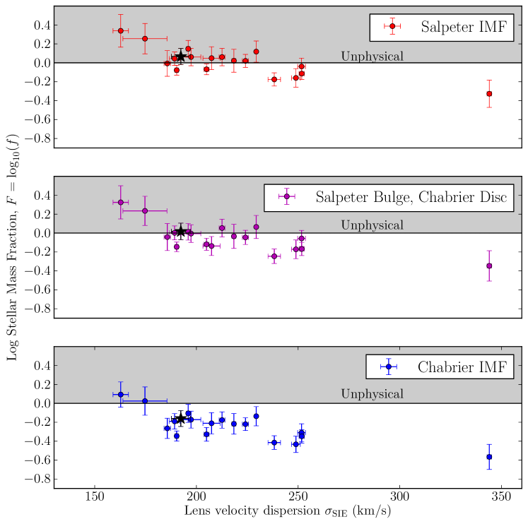
Figure 1: A comparison of the “observed” stellar mass fraction as a function of lens velocity dispersion for three different IMF scenarios. The vertical error bars are approximate, and were computed by calculating the uncertainty in the ratio of the stellar mass to the total mass assuming those two quantities are independent. The top two panels are similar to plots from SWELLS-III, while the middle panel is new to this paper. Top: Salpeter IMF, Middle: Salpeter IMF for bulge, Chabrier IMF for disc, Bottom: Chabrier IMF. The galaxy denoted with the black star symbol is J0820$+$4847, which is the object studied in Section 5.

In Figure 1, we plot, as a function of the estimated value of the gravitational lens velocity dispersion parameter $\widetilde{\sigma_{\mathrm{SIE}}}$, the “observed” mass fraction in stars, calculated naïvely by dividing the measured stellar mass by the measured total mass:

$$F\approx\log_{10}\left(10^{\widetilde{\mathcal{M}_{\rm b}}+\widetilde{\mathcal{M}_{\rm d}}}\right)-\widetilde{M_{\rm tot}}$$ (7)

In the top panel, we see the assumption of a Salpeter IMF leads to a prediction of high stellar mass fraction, and many of the galaxies in our sample appear in the unphysical region $F>0$ (or $f>1$). Thus, this data set seems to provide some evidence against the Salpeter IMF, and “heavier” IMFs, for this sample. Our goal in the remainder of this paper is to formalise this intuition by carefully performing the inference and obtaining constraints on hypotheses about the IMF normalisations $\alpha$ for the bulges and discs in this sample. This will be achieved by a Bayesian analysis of the data given in Table 1. This analysis should be considered as superseding the one presented in SWELLS-III.

5 A Single Galaxy

5.1 Noise-Free Argument

In this section we describe a simple argument for constraining the IMF normalisation parameters $\alpha_{\rm b}$ and $\alpha_{\rm d}$ in a single galaxy based on an SPS mass measurement (that assumed a Salpeter IMF) and a total mass measurement. This simple argument provides the fundamental reason for why this data set can constrain the IMF, free of the later probabilistic complications.

Suppose that the log of the total mass of a galaxy (within some aperture, in our case the elliptical critical curve of each system’s lens model) has been measured exactly (without noise), giving the result

$$M_{\rm tot} = \log_{10}\left(m_{\rm b}+m_{\rm d}+m_{\rm h}\right).$$ (8)

Suppose also that the bulge mass and the disc mass within the same aperture have also been measured exactly from the galaxy photometry and the application of an SPS model that assumes a Salpeter IMF. This is equivalent to having obtained the values of the following “SPS masses:”

$$\mathcal{M}_{\rm b} = \log_{10}\left(\frac{m_{\rm b}}{\alpha_{\rm b}}\right)$$ (9)

$$\mathcal{M}_{\rm d} = \log_{10}\left(\frac{m_{\rm d}}{\alpha_{\rm d}}\right).$$ (10)

In terms of these quantities, the total stellar mass (bulge plus disc) within the aperture is:

$$m_{\rm b}+m_{\rm d} = \alpha_{\rm b}10^{\mathcal{M}_{\rm b}}+\alpha_{\rm d}10^{\mathcal{M}_{\rm d}}.$$ (11)

The key argument is that the total stellar mass cannot be greater than the total mass including dark matter. This leads to the following constraint:

$$m_{\rm b}+m_{\rm d} \leq m_{\rm tot}$$ (12)

$$\alpha_{\rm b}10^{\mathcal{M}_{\rm b}}+\alpha_{\rm d}10^{\mathcal{M}_{\rm d}} \leq 10^{M_{\rm tot}}.$$ (13)

Equation 13 can be interpreted as a linear constraint on $\alpha_{\rm b}$ and $\alpha_{\rm d}$. This constraint, produced under the (false) assumption of noise-free measurements, is plotted as the dotted green line in Figure 2, alongside more justified conclusions derived henceforth.

5.2 Inference in the Presence of Noise

The assumption of noise-free measurements above is of course invalid. We now relax this assumption in order to obtain a probabilistic version of the constraint Equation 13.

Bayesian inference provides the framework for inferring the values of unknown model parameters. This is done by assuming a prior distribution ${\rm Pr}(\theta)$ over the parameter space (where $\theta$ denotes the unknown parameters) and updating this to a posterior distribution using Bayes’ rule:

$${\rm Pr}(\theta|D)\propto{\rm Pr}(\theta){\rm Pr}(D|\theta).$$ (14)

The first ingredient for the analysis is a choice of prior distribution ${\rm Pr}(\theta)$ describing initial uncertainty about the parameter values. The second ingredient for the analysis is a choice of “sampling distribution” ${\rm Pr}(D|\theta)$ which describes our assumptions about how the data came about, or our predictions about data we would be likely to observe if we happened to know the values of the unknown parameters. When the data are fixed the sampling distribution is a function of the parameters only, called the likelihood function. If the set of possible values for $\theta$ and $D$ is continuous then ${\rm Pr}(\theta)$ and ${\rm Pr}(D|\theta)$ are probability density functions (PDFs).

At this point we note a common misconception: that priors are subjective and sampling distributions are somehow measurable. In fact, both priors and sampling distributions describe prior beliefs (which may be informed by previous data). The prior ${\rm Pr}(\theta)$ models an agent’s prior beliefs about the values of the parameters, and the sampling distribution ${\rm Pr}(D|\theta)$ models the agent’s prior beliefs about how the data are related to the parameters. Without prior knowledge of a relationship, inference is not possible.

The final ingredients in the analysis are the actual data $D$ and numerical methods (such as Markov Chain Monte Carlo [MCMC]) for computing the posterior distribution ${\rm Pr}(\theta|D)$ or summaries thereof.

5.2.1 Data

In our case, the data are the values of the three measured quantities:

$$D=\{\widetilde{\mathcal{M}_{\rm b}},\widetilde{\mathcal{M}_{\rm d}},\widetilde{M_{\rm tot}}\}.$$ (15)

In principle, a more “raw” version of the data, such as pixel values, should be used. However, this is prohibitive in many applications.

For concreteness we will use the galaxy SWELLS J0820$+$4847 to demonstrate the technique. This galaxy has the following mass measurements within its critical curve:

$$\begin{array}[]{lllll}\widetilde{\mathcal{M}_{\rm b}}&=&10.65\\ \widetilde{\mathcal{M}_{\rm d}}&=&10.15\\ \widetilde{M_{\rm tot}}&=&10.71.\end{array}$$ (16)

The uncertainties on these measurements are:

$$\begin{array}[]{lllll}\sigma_{\rm b}&=&0.09\\ \sigma_{\rm d}&=&0.08\\ \sigma_{\rm tot}&=&0.05.\end{array}$$ (17)

These estimates and uncertainties are the result of SPS modelling (in the case of $\mathcal{M}_{\rm b}$ and $\mathcal{M}_{\rm d}$) and gravitational lens modelling (in the case of $M_{\rm tot}$).

5.2.2 Sampling Distribution

We make the usual Gaussian (normal) assumption for the measured quantities given the true quantities:

$$\begin{array}[]{lllll}\widetilde{\mathcal{M}_{\rm b}}&\sim&\textnormal{Normal}\left(\mathcal{M}_{\rm b},\sigma_{\rm b}^{2}\right)\\ \widetilde{\mathcal{M}_{\rm d}}&\sim&\textnormal{Normal}\left(\mathcal{M}_{\rm d},\sigma_{\rm d}^{2}\right)\\ \widetilde{M_{\rm tot}}&\sim&\textnormal{Normal}\left(M_{\rm tot},\sigma_{\rm tot}^{2}\right).\end{array}$$ (18)

5.2.3 Parameters and Priors

The unknown parameters of interest to be inferred are $\alpha_{\rm b}$ and $\alpha_{\rm d}$. However, the sampling distributions in Equation 18 depend on the values of the unknown nuisance parameters $\mathcal{M}_{\rm b}$, $\mathcal{M}_{\rm d}$ and $M_{\rm tot}$, so they must also be included as model parameters. For convenience, rather than using $M_{\rm tot}$ as a parameter we will parameterise in terms of $F$, which so our five unknown parameters are:

$$\theta=\left\{\alpha_{\rm b},\alpha_{\rm d},\mathcal{M}_{\rm b},\mathcal{M}_{\rm d},F\right\}$$ (19)

Therefore, the final line of the sampling distributions (Equation 18) will need to be written in terms of these parameters. Note that:

$$m_{\rm tot} = \frac{m_{\rm b}+m_{\rm d}}{f}$$ (20)

Which implies:

$$M_{\rm tot} = \log_{10}\left(\alpha_{\rm b}10^{\mathcal{M}_{\rm b}}+\alpha_{\rm d}10^{\mathcal{M}_{\rm d}}\right)-F$$ (21)

Therefore, the final line of the likelihood (Equation 18) can be rewritten in terms of the parameters $\theta$:

$$\widetilde{M_{\rm tot}}\sim\textnormal{Normal}\left(\log_{10}\left(\alpha_{\rm b}10^{\mathcal{M}_{\rm b}}+\alpha_{\rm d}10^{\mathcal{M}_{\rm d}}\right)-F,\sigma_{\rm tot}^{2}\right)$$ (22)

To assign priors, we can use broad distributions that allow a wide range of plausible values. For $\alpha_{\rm b}$ and $\alpha_{\rm d}$ we use a plausible range from 0.3 to 2. Let us also (for now) assume that we know “almost nothing” about the masses of galaxies, but guess that each component’s mass (assuming a Salpeter IMF) lies somewhere between $10^{5}$ and $10^{15}$ solar masses. This is a very broad prior range and a much narrower prior would be astrophysically justified, however, the prior range does not have much of an effect because these quantities are directly measurable and the posterior distribution will be much narrower than the prior.

This prior information is encoded by the following choices for the prior distribution (for four of the five parameters):

$$\alpha_{\rm b} \sim \textnormal{Uniform}(0.3,2)$$ (23)

$$\alpha_{\rm d} \sim \textnormal{Uniform}(0.3,2)$$ (24)

$$\mathcal{M}_{\rm b} \sim \textnormal{Uniform}(5,15)$$ (25)

$$\mathcal{M}_{\rm d} \sim \textnormal{Uniform}(5,15)$$ (26)

The final parameter that requires a prior distribution is $F$. This variable naturally has an upper limit of zero, and we shall assign a uniform prior:

$$F \sim \textnormal{Uniform}(-5,0).$$ (27)

Other quantities that may be of interest are considered derived quantities and can be obtained from the formulae given in Section 3.

The choice of uniform priors, particularly for $\alpha_{\rm b}$ and $\alpha_{\rm d}$, is not intended to be a realistic description of the best judgment of an IMF expert. Rather, the uniform prior is a convenient choice that allows us to easily see the effect of the current data set in the results.

5.2.4 Computation

To obtain the marginal distributions for $\alpha_{\rm b}$ and $\alpha_{\rm d}$ we implemented this model in the JAGS program for MCMC (Plummer, 2003). JAGS was chosen because it is straightforward to implement complex Bayesian models using its model specification language. For this study, this attribute was more important than computational efficiency.

6 Results: the bulge and disc IMFs in a single galaxy

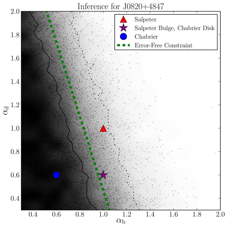
Figure 2: The posterior PDF for the bulge and disc IMF normalisation parameters $\alpha_{\rm b}$ and $\alpha_{\rm d}$ for SWELLS J0820$+$4847. Darker regions have higher probability density. If noise-free measurements were available, the green dotted line would provide a hard limit. The presence of noise has smoothed out the constraint, so that more massive IMFs become less plausible in a gradual manner. Note that the bulge IMF is more constrained than the disc IMF. This occurs because the bulge has more mass within the critical curve than the disc. The inner contour encloses 68% of the probability and the outer contour encloses 95%. The hypothesis that both bulge and disc IMF normalisations are Salpeter is indicated by the red triangle at (1, 1). Similarly, the purple star at (1, 0.6) and the blue circle at (0.6, 0.6) denote other hypotheses about the IMF of the bulge and the disc in SWELLS J0820$+$4847.

Figure 2 shows the posterior PDF for the bulge and disc IMF normalisations, $\alpha_{\rm b}$ and $\alpha_{\rm d}$, given the SWELLS J0820$+$4847 data. For clarity, the dotted line shows the constraint that would be obtained from Equation 13 if the measurements had zero uncertainty (Section 5.2; note the perfect degeneracy between the bulge and disc IMF normalisations). The posterior is approximately uniform below the constraint line, just like the prior. As expected, the probabilistic model has softened the hard constraint. We see that $\alpha_{\rm b}$ is more constrained than $\alpha_{\rm d}$, a result of the fact that this lens is dominated by the bulge, within its critical curve (as are most of the SWELLS lenses). We find that, under these assumptions, and marginalising over all other parameters, $\alpha_{\rm b}<1.10$ with 95% probability. For comparison, the prior probability of the hypothesis $\alpha_{\rm b}<1.10$ was 47%.

7 A hierarchical model

We now consider the simultaneous analysis of multiple galaxies in order to produce stronger constraints than those produced in the single system SWELLS J0820$+$4847 and shown in Figure 2. It is tempting to simply repeat the analysis of Section 5 for each system and take the product of the resulting marginal likelihood as a function of $\alpha_{\rm b}$ and $\alpha_{\rm d}$. However, such an approach would produce innaccurate results due to the following hidden assumptions. Firstly, in this approach we would be implicitly assuming that there is one $\alpha_{\rm b}$ value that applies to all bulges and one $\alpha_{\rm d}$ value that applies to all discs. Secondly (and more importantly), the model in Section 5 assumes a broad prior on the logarithm of the stellar mass fraction ($F$). Applying this model to every galaxy is equivalent to assuming the prior on the set of $F$-values ($\{F^{j}\}$) is independent. This assumption is problematic because it implies that the $F$ values are all very likely to be scattered across the whole range $[-5,0]$ and are very unlikely to be concentrated together.

Thus, the prior probability that (for example) all objects have a high stellar mass fraction is unreasonably low, and the model will favour lower values for the IMF normalisation. Inspection of Figure 1 suggests that a universal Salpeter IMF should be disfavoured; however the strength of this conclusion will depend strongly on how plausible it is that most galaxies in the sample have high stellar mass fractions. Applying the Section 5 analysis independently to each object implies a very small prior probability for all galaxies having approximately the same high $F$ value, while we have no good reasons to be sceptical of this possibility. In other words, such an analysis ignores our belief that some common physical framework is responsible for the formation and evolution of all galaxies. The result from applying this strategy is shown in Appendix C.

To overcome these problems, we introduce an alternative hierarchical Bayesian model. We allow each galaxy to have its own value for $\alpha_{\rm b}$ and its own value for $\alpha_{\rm d}$, but rather than assigning independent Uniform$(0.3,2)$ priors for these parameters, we assume that the prior would be a lognormal distribution, if only we knew the appropriate mean and variance. However, we do not know the appropriate mean and variance, so we allow those to be unknown parameters as well. There are several ways to parameterise a lognormal distribution. Throughout this paper we use the median value $\mu$ of the variable and the standard deviation of the natural logarithm of the variable, denoted by $\sigma$. The lognormal density for a variable $x$ is given by:

$${\rm Pr}(x|\mu,\sigma) = \frac{1}{x\sigma\sqrt{2\pi}}\exp\left[-\frac{1}{2\sigma^{2}}\left(\ln(x)-\ln(\mu)\right)^{2}\right]$$ (28)

for $x\geq 0$. When applied to the bulge IMF normalisations, the hierarchical prior increases the prior probability that the $\alpha_{\rm b}$ values are very similar to each other across the population and encodes our belief that the physics of star formation is not wildly different in different galaxies. The median and variance of this phenomenological model for the distribution of bulge IMFs are to be inferred from the data. Similarly, we take the $\alpha_{\rm d}$ parameters of each disc to be drawn from a different lognormal distribution. We now have four hyperparameters that represent our simple model for the distribution of bulge and disk IMFs in the population. It is to these hyperparameters – the medians and variances of the conditional prior PDFs for the $\alpha_{\rm b}$ and $\alpha_{\rm d}$ parameters – we assign vague, “uninformative” priors. The $\{\alpha_{\rm b}^{j}\}$ and $\{\alpha_{\rm d}^{j}\}$ variables are not the only quantities whose prior should be modified when the model is extended to multiple galaxies. We shall assume the bulge “masses” $\{\mathcal{M}_{\rm b}^{j}\}$ were drawn from a common normal distribution, whose mean $\mu_{\mathcal{M}_{\rm b}}$ and width $\sigma_{\mathcal{M}_{\rm b}}$ we hope to infer from the sample. This corresponds to the assumption that our galaxies’ bulges are similar in their mass, which makes sense given that they were all selected in the same way (Treu et al., 2011). We make the same assumption for the discs: that they are similar in their mass. This introduces additional hyperparameters $\mu_{\mathcal{M}_{\rm d}}$ and $\sigma_{\mathcal{M}_{\rm d}}$.

Each of our galaxies has an $F$ value, the logarithm (base 10) of the fraction of the mass that is in stars (within its critical curve). Rather than applying a simple hierarchical structure to the prior on the $\{F^{j}\}$ variables, the apparent trend in Figure 1 motivates the assumption that the $F$ values for the galaxies vary as a function of $\widetilde{\sigma_{\mathrm{SIE}}}$. The hard upper limit of $F=0$ complicates matters, so we work in the logit basis where $\ell=\ln\left[f/(1-f)\right]$. We shall assume that the mass fractions are scattered around the following relationship as a function of $\log_{10}\left(\widetilde{\sigma_{\mathrm{SIE}}^{j}}\right)$:

$$\ell = \ell_{0}+\ell_{1}\log_{10}\left[\frac{\widetilde{\sigma_{\mathrm{SIE}}^{j}}}{162.8\textnormal{ km/s}}\right].$$ (29)

In this relationship, $\ell_{0}$ is the “initial” value of the trend line, $\ell_{1}$ is the gradient, and 162.8 km/s is the lowest $\widetilde{\sigma_{\mathrm{SIE}}^{j}}$ value in the data set, where $\ell=\ell_{0}$ applies. This assumption introduces hyperparameters $\ell_{0}$, $\ell_{1}$ and $\sigma_{\ell}$ into the model, where the latter is the degree of scatter around the assumed trend line. We choose vague priors for $\ell_{0}$ and $\sigma_{\ell}$. For $\ell_{1}$ (the slope of the trend), we choose a heavy tailed Cauchy (Lorentzian) distribution centered at 0 and with a scale of 10. This models a prior assumption that $\ell_{1}$ is probably small in magnitude (such that we would not expect $\ell$ to vary by more than 10 over an order-of-magnitude range of $\widetilde{\sigma_{\mathrm{SIE}}^{j}}$), but the heavy tails allow this assumption to be incorrect if the data warrant it.

The prior PDF for all hyperparameters and parameters, and the sampling distribution for the data given the parameters, is given in Table 2. The structure of this hierarchical model is depicted graphically in Figure 3. This diagram can be understood as a recipe for generating simulated data sets by working from the outer nodes (hyperparameters) to the innermost data nodes. The first step would be to generate hyperparameter values from their prior, to describe the central tendencies and diversities of the galaxies’ properties. Then, individual galaxy properties would be drawn from their distributions given the hyperparameters. Finally, data values would be generated from the sampling distributions given the individual galaxy properties. A recipe for simulating data (starting by simulating parameter values from their prior) is equivalent to a fully specified Bayesian model. In Section 8 we present the results from the SWELLS sample.

Parameter	Meaning	Probability Distribution
Population Hyperparameters
$\mu_{\alpha_{\rm b}}$	Median of bulge IMFs	Uniform(0.3, 2)
$\sigma_{\alpha_{\rm b}}$	Diversity of bulge IMFs	LogUniform(0.001, 1)
$\mu_{\alpha_{\rm d}}$	Median of disc IMFs	Uniform(0.3, 2)
$\sigma_{\alpha_{\rm d}}$	Diversity of disc IMFs	LogUniform(0.001, 1)
$\mu_{\mathcal{M}_{\rm b}}$	Median of bulge masses	Uniform(5, 15)
$\sigma_{\mathcal{M}_{\rm b}}$	Diversity of bulge masses	LogUniform(0.001, 1)
$\mu_{\mathcal{M}_{\rm d}}$	Median of disc masses	Uniform(5, 15)
$\sigma_{\mathcal{M}_{\rm d}}$	Diversity of disc masses	LogUniform(0.001, 1)
$\ell_{0}$	Median of $\ell$ (logit-transformed $f$) at $\widetilde{\sigma_{\mathrm{SIE}}}=162.8$ km/s	Uniform(-10, 10)
$\ell_{1}$	Gradient of $\ell$ trend with $\log_{10}\left(\widetilde{\sigma_{\mathrm{SIE}}}\right)$	Cauchy(0, 10)
$\sigma_{\ell}$	Scatter of $\ell$ values around trend line	LogUniform(0.001, 1)
Individual Galaxy Parameters
$\alpha_{\rm b}^{j}$	Bulge IMF	LogNormal($\mu_{\alpha_{\rm b}}$, $\sigma_{\alpha_{\rm b}}^{2}$)
$\alpha_{\rm d}^{j}$	Disc IMF	LogNormal($\mu_{\alpha_{\rm d}}$, $\sigma_{\alpha_{\rm d}}^{2}$)
$\mathcal{M}_{\rm b}^{j}$	log10(“Salpeter” Bulge mass)	$\textnormal{Normal}(\mu_{\mathcal{M}_{\rm b}},\sigma_{\mathcal{M}_{\rm b}}^{2})$
$\mathcal{M}_{\rm d}^{j}$	log10(“Salpeter” Disc mass)	$\textnormal{Normal}(\mu_{\mathcal{M}_{\rm d}},\sigma_{\mathcal{M}_{\rm d}}^{2})$
$\ln\left(\frac{f^{j}}{1-f^{j}}\right)$	logit-transformed stellar mass fraction	$\textnormal{Normal}\left(\ell_{0}+\ell_{1}\log_{10}\left[\frac{\widetilde{\sigma_{\mathrm{SIE}}^{j}}}{162.8\textnormal{ km/s}}\right],\sigma_{\ell}^{2}\right)$
Data
$\widetilde{\mathcal{M}_{\rm b}^{j}}$	SPS bulge mass measurement	$\textnormal{Normal}(\mathcal{M}_{\rm b}^{j},(\sigma_{\rm b}^{j})^{2})$
$\widetilde{\mathcal{M}_{\rm d}^{j}}$	SPS disc mass measurement	$\textnormal{Normal}(\mathcal{M}_{\rm d}^{j},(\sigma_{\rm d}^{j})^{2})$
$\widetilde{M_{\rm tot}^{j}}$	Lensing total mass measurement	$\textnormal{Normal}\left(\log_{10}\left(\alpha_{\rm b}^{j}10^{\mathcal{M}_{\rm b}^{j}}+\alpha_{\rm d}^{j}10^{\mathcal{M}_{\rm d}^{j}}\right)-F^{j},(\sigma_{\rm tot}^{j})^{2}\right)$

Table 2: All the parameters in our hierarchical model, with their assigned prior PDFs or sampling distributions. In our notation for a lognormal distribution, the first entry gives the median or central value of the variable, and the second entry gives the variance (standard deviation squared) of the natural log of the variable. However, the variance is usually written as $\sigma^{2}$ so the standard deviation can be read easily. The total number of unknown parameters and hyperparameters is 106 and the total number of measurements is 57 (not including noise variances on the measurements, which are counted as prior information).

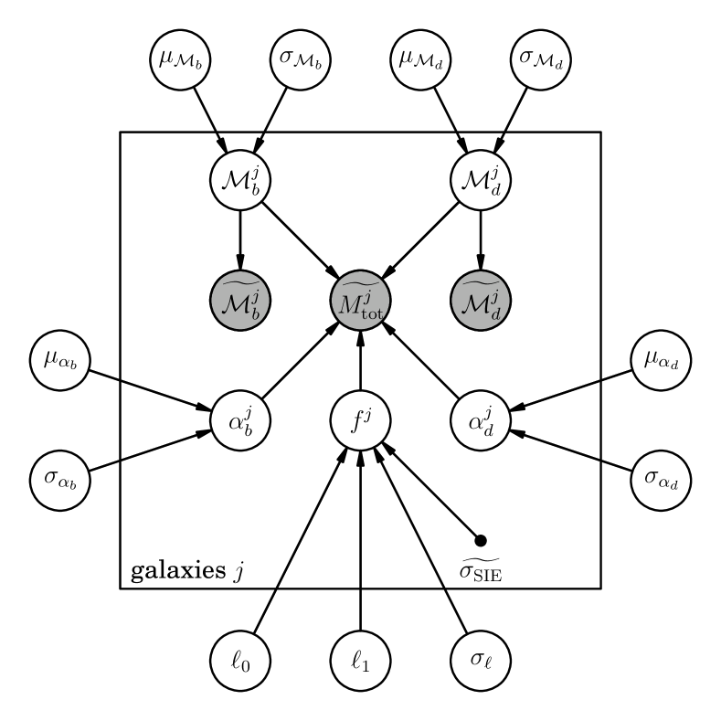
Figure 3: Probabilistic graphical model of our hierarchical model, produced using the DAFT package by Dan Foreman-Mackey and David Hogg, available from http://daft-pgm.org/. The equations illustrated by this figure are given in Table 2. The box can be interpreted as a ‘for’ loop, indicating quantities that are defined for each lens galaxy in the sample. Shaded nodes denote observed quantities (aka “data”) whose values are conditioned on in the inference. The small black dot indicates quantities that are fixed and known, but considered as “prior information” rather than “data” (i.e. no sampling distribution is specified).

8 Results: the disc and bulge IMFs in the SWELLS sample

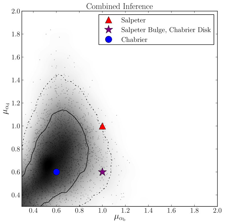
Figure 4: Samples from the posterior PDF for the median IMF normalisation parameters in the context of our hierarchical model, $\mu_{\alpha_{\rm b}}$ and $\mu_{\alpha_{\rm d}}$, given 19 SWELLS galaxies’ mass measurements. The inner contour encloses 68% of the probability and the outer contour encloses 95%. The hypothesis that both bulge and disc IMF normalisations are centered around Salpeter is indicated by the red triangle at (1, 1). Similarly, the purple star at (1, 0.6) and the blue circle at (0.6, 0.6) denote other hypotheses about the typical IMFs of bulges and discs.

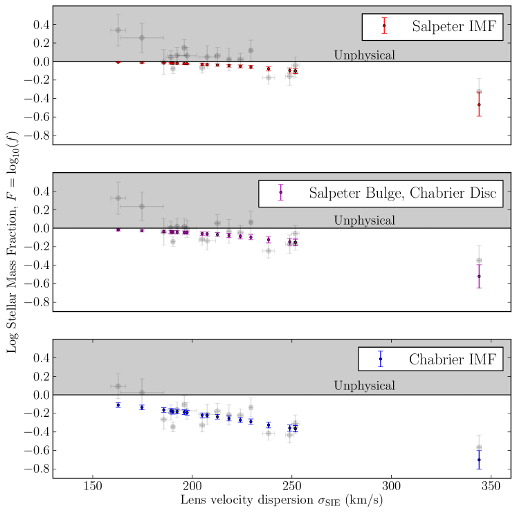
Figure 5: The inferred stellar mass fractions $F$ from the inference, for comparison with Figure 1. The “observed” (and often unphysical) $F$ values are plotted as grey points, while the hierarchically-inferred $F$ values are shown in colour. Top: Salpeter IMF, Middle: Salpeter IMF for bulge, Chabrier IMF for disc, IMF: Bottom: Chabrier IMF.

The hierarchical model specified in Section 7 was implemented and run in JAGS, producing posterior samples for all of the hyperparameters and parameters listed in Table 2. To investigate conclusions similar to those for SWELLS J0820$+$4847 in Figure 2, we plot the marginal posterior PDF for $\mu_{\alpha_{\rm b}}$ and $\mu_{\alpha_{\rm d}}$ in Figure 4. We see that in this sample, the mass measurements tend to support light IMFs in both the disc and the bulge components. The constraint on the bulge IMF is marginally tighter than the disc constraint, as we might expect for these brighter, more massive galaxy components. Heavy IMFs are somewhat disfavoured for both components in these galaxies: marginalising, we find that ${\rm Pr}(\mu_{\alpha_{\rm b}}<1)\approx 96.6\%$ while ${\rm Pr}(\mu_{\alpha_{\rm d}}<1)\approx 81.6\%$. The prior probability of each of these hypotheses was 41.2%. In other words, this data strongly disfavours the hypothesis that the centroid of the distribution of $\alpha$ values is greater than Salpeter (1). However, the assumption of a near-universal IMF ($\mu_{\alpha_{\rm b}}\approx\mu_{\alpha_{\rm d}}$ and both $\sigma_{\alpha_{\rm b}}$ and $\sigma_{\alpha_{\rm d}}$ are small) is compatible with the data.

Figure 4 shows the posterior distribution for the median IMF normalisations for bulges and disks, but we have assumed that there is some (possibly small) diversity in $\alpha_{\rm b}$ and $\alpha_{\rm d}$ from galaxy to galaxy. We plot the posterior PDF for the width parameters $\sigma_{\alpha_{\rm b}}$ and $\sigma_{\alpha_{\rm d}}$ in Figure 6. Note that the axes in this plot are in logarithmic units, so that the assumed prior was uniform inside the square shown. The data have ruled out the upper and right-most parts of this space, and are consistent with values in the lower left quadrant. A perfect universal IMF would imply (among other things, such as $\mu_{\alpha_{\rm b}}=\mu_{\alpha_{\rm d}}$) that $\sigma_{\alpha_{\rm b}}=\sigma_{\alpha_{\rm d}}=0$, and this is not included in our hypothesis space. However, low but nonzero values of $\sigma_{\alpha_{\rm b}}$ and $\sigma_{\alpha_{\rm d}}$ may be considered close enough to zero for practical purposes, but probability statements about universality would be sensitive to the definition. Marginalising over all other hyperparameters and parameters, we find 95% upper limits by computing ${\rm Pr}(\sigma_{\alpha_{\rm b}}\leq 0.165)=95\%$ and ${\rm Pr}(\sigma_{\alpha_{\rm d}}\leq 0.375)=95\%$. The prior probabilities of these two hypotheses were 55% and 64% respectively.

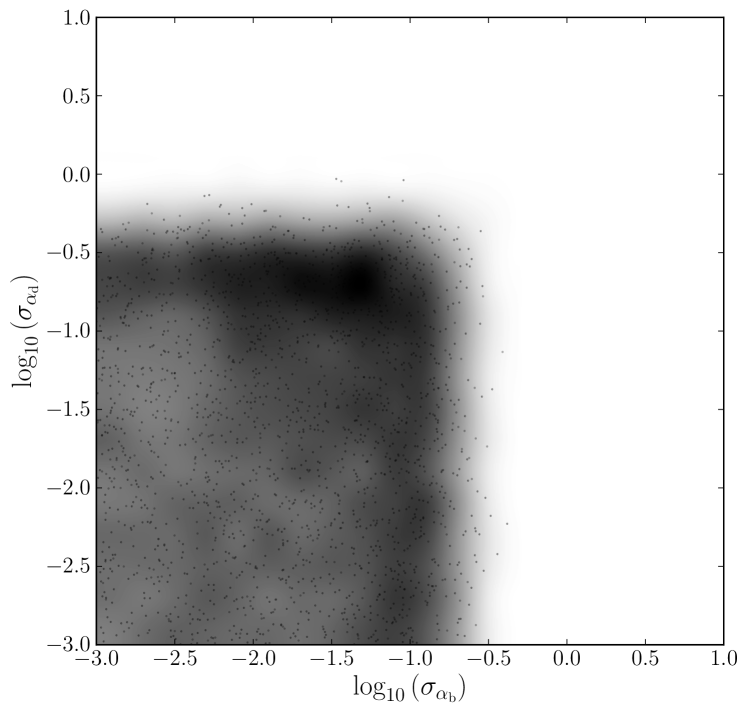
Figure 6: Samples from the posterior PDF for the width parameters, $\sigma_{\alpha_{\rm b}}$ and $\sigma_{\alpha_{\rm d}}$, of the galaxy component IMF normalisation distributions, given 19 SWELLS galaxies’ mass measurements. Small values of $\sigma_{\alpha_{\rm b}}$ imply a situation where the IMFs of bulges are close to universal, and this is not ruled out by the data. This is also the case with $\sigma_{\alpha_{\rm d}}$. The prior was uniform over the square region plotted here, so the data merely rule out high values of the width parameters.

The galaxy stellar mass fractions inferred in this hierarchical model are plotted in Figure 5, where the error bars represent the full uncertainty in the masses after marginalising over $\alpha_{\rm b}$ and $\alpha_{\rm d}$ for that galaxy, and also over the population hyper-parameters.

To make this plot we repeated the inference while conditioning on the Chabrier/Salpeter models by setting $\mu_{\alpha_{\rm b}},\mu_{\alpha_{\rm d}}=(0.6,0.6),(0.6,1),(1,1)$ and $(\sigma_{\alpha_{\rm b}},\sigma_{\alpha_{\rm d}})=(0,0)$. As opposed to Figure 1 it can be immediately noted that none of the inferred stellar mass fractions are unphysical, and that all have smaller uncertainties than the simply-estimated “observed” mass fractions; this latter point results from the fact that our model correlates each of the lenses and penalises widely discrepant masses, thereby reducing the uncertainties. In each case, we see a significant trend of lower stellar mass fractions in galaxies with increasing total mass (as represented by $\sigma_{\mathrm{SIE}}$). This could be due to the dark matter fraction increasing as the Einstein radius increases and the mass enclosed becomes less dominated by the stars.

9 Discussion and Conclusions

We have implemented a hierarchical model for a sample of strong lens galaxies, and used it to interpret a set of highly compressed data: total mass estimates obtained from strong gravitational lensing, and stellar mass estimates of the bulge and disc components obtained from SPS models that assume a Salpeter IMF. This simple set-up allowed us to explore the basic mechanics of the hierarchical inference in some detail. We found that an apparently uninformative prior on each galaxy component mass can actually have a significant impact on the results, since this assignment opens up an exponentially large volume of nuisance parameter space. A hierarchical prior on the masses as well stabilises the problem, as well as matching our actual knowledge of a) our selection process and b) galaxies in general. Further work on higher fidelity data might profitably include some relaxing of our assumptions of simple log-normal distributions for both the component masses and the $\alpha$ parameters.

While the data set analysed here is only a small subset of all the available information about variations of the IMF, it is an instructive subset that demonstrates many of the issues that arise when combining small amounts of information from large numbers of objects. In particular, the assumptions about the prior distributions for nuisance parameters are extremely important: assuming independence can lead to absurd conclusions. We also note that scepticism of IMF variations (e.g. Bastian, Covey, & Meyer, 2010) must eventually break down at some point as the only truly universal IMF would be one composed of delta function spikes at the true initial mass of each actual star in the universe: in other words, the appropriate question is not “does the IMF vary” but “how much does the IMF vary, and as a function of what parameters?”. Ultimately, detailed models of individual SWELLS galaxies, taking into account all of the available data (Barnabè et al., 2012) could be combined in similar way to the analysis of this paper. This would lead to a full description of the conclusions of the SWELLS survey: not only about the properties of the IMFs of disk galaxies but also about all other properties measurable from gravitational lensing and dynamical measurements.

While the analysis in this paper is something of a toy model, it does achieve some important goals. First, we have replaced the rather unsatisfactory “observed stellar mass fractions” that appeared in SWELLS-III, and in the process, incorporated some new, quantitative information – the fact that stellar mass fractions cannot be greater than one – into the inference of IMF normalisation. Second, the hierarchical framework we have presented has allowed us to explore the model that we were actually interested in! If we are to relax the assumption of a Universal IMF, that means that each galaxy must have a different IMF, each of which is to be measured. The hierarachical model enables investigation of all possible scenarios in between the two extremes of Universality and total randomness. It seems to us that asserting some distribution of IMF parameters, implying some essential similarity between galaxies in a sample, is the logical first step beyond universality.

Our conclusions regarding the IMF normalisation in the bulge and disc components of our sample of galaxies can be stated as follows:

• Under the assumptions that 1) the stellar populations of a particular bulge or disc can each be described by a single IMF normalisation, and 2) that bulges are drawn from one population distribution (both in stellar mass and IMF normalisation) and discs another, we find that the galaxies in the SWELLS sample seem to have been drawn from a sub-population with lighter-than Salpeter IMF: the medians of the bulge and disc IMF normalisation distribution are such that $p(\mu_{\alpha_{\rm b}}<1)\approx 96.6\%$ while $p(\mu_{\alpha_{\rm d}}<1)\approx 81.6\%$.

• The widths of the distributions of IMF normalisations are consistent with small values (i.e. a close-to-universal IMF) or more moderate values (variable IMF), both for SWELLS galaxy bulges and SWELLS galaxy discs. Given the uncertainty in the measurements, we cannot draw firm conclusions about IMF universality from these parameters alone, despite them being the natural choice. The results are consistent with the hypothesis of a universal IMF, but not a universal Salpeter IMF.

We suggest that hierarchical modelling is the natural way to approach inference problems involving samples of complex objects which can be assumed to be similar in certain respects. In particular, as samples of strong lenses continue to grow, we expect these highly informative individual objects to be most informative in ensembles when analysed in this way.

Appendix A Probability Expressions

Here we discuss the independence assumptions used in the hierarchical model specified in Section 7. The unknown hyperparameters (which describe the population distributions) are:

$$\boldsymbol{\eta}=\left\{\mu_{\alpha_{\rm b}},\sigma_{\alpha_{\rm b}},\mu_{\alpha_{\rm d}},\sigma_{\alpha_{\rm d}},\mu_{\mathcal{M}_{\rm b}},\sigma_{\mathcal{M}_{\rm b}},\mu_{\mathcal{M}_{\rm d}},\sigma_{\mathcal{M}_{\rm d}},\ell_{0},\ell_{1},\sigma_{\ell}\right\}$$ (30)

The priors on these hyperparameters are given in Table 2. The parameters for an individual galaxy $j$ are:

$$\boldsymbol{\theta}^{j}=\left\{\alpha_{\rm b}^{j},\alpha_{\rm d}^{j},\mathcal{M}_{\rm b}^{j},\mathcal{M}_{\rm d}^{j},f^{j}\right\}.$$ (31)

The joint prior for all unknown hyperparameters and the individual galaxy parameters can be written using the product rule:

$${\rm Pr}\left(\boldsymbol{\eta},\left\{\boldsymbol{\theta}^{j}\right\}_{j=1}^{N}\right) = {\rm Pr}\left(\boldsymbol{\eta}\right){\rm Pr}\left(\left\{\boldsymbol{\theta}^{j}\right\}_{j=1}^{N}|\boldsymbol{\eta}\right)$$ (32)

The assumption is that, given the hyperparameters, the individual galaxy parameters are independent:

$${\rm Pr}\left(\boldsymbol{\eta},\left\{\boldsymbol{\theta}^{j}\right\}_{j=1}^{N}\right) = {\rm Pr}\left(\boldsymbol{\eta}\right)\prod_{i=1}^{N}{\rm Pr}\left(\boldsymbol{\theta}^{j}|\boldsymbol{\eta}\right)$$ (33)

where ${\rm Pr}\left(\boldsymbol{\theta}^{j}|\boldsymbol{\eta}\right)$ is the same function for each $j$. We also assume that the data for galaxy $j$ is independent and only depends on the parameters for galaxy $j$:

$${\rm Pr}\left(\mathbf{D}|\boldsymbol{\eta},\boldsymbol{\theta}\right) = \prod_{i=1}^{N}{\rm Pr}\left(\mathbf{D}^{j}|\boldsymbol{\theta}^{j}\right)$$ (34)

where ${\rm Pr}\left(\mathbf{D}^{j}|\boldsymbol{\theta}^{j}\right)$ is the same function for all $j$.

One way to think about the hierarchical model is to think of the hyperparameters as describing the distribution of galaxy properties in the population, and each galaxy as being a point “drawn from” this distribution. The data is then drawn independently (for each galaxy) from a distribution that is dependent only on that galaxy’s properties, and not on the properties of that galaxy or the hyperparameters. These assumptions make sense when the objects being studied can literally be thought of as having been sampled from some population. However, hierarchical models can also be used when there is no population. Introducing the hyperparameters is a convenient way of constructing a prior distribution for $N$ exchangeable variables that are dependent. One could imagine marginalising away the hyperparameters which would give a dependent prior on the parameters (such that, for example, knowledge of several galaxies’ properties would be informative about the properties of a subsequent galaxy). hierarchical models can be used to implement such dependent priors, even when the “population” motivation may be absent.

Appendix B Corner/Triangle Plot

For completeness, a “corner” plot, showing various joint posterior distributions for an interesting subset of the hyperparameters, is given in Figure 7. A distinct correlation exists between $\ell_{0}$ and $\mu_{\alpha_{\rm b}}$, and $\ell_{0}$ and $\mu_{\alpha_{\rm d}}$, reflecting the fact that higher stellar mass fractions enable the IMF normalisation to be increased somewhat before becoming incompatible with the data. This plot was made using triangle.py by Dan Foreman-Mackey, available from http://www.github.com/dfm/triangle.py.

Figure 7: A “corner” plot of joint posterior distributions for many of the hyperparameters.

Appendix C Non-hierarchical Results

The results obtained by applying the single-object model (Section 5) to all 19 galaxies in the sample, and then combining the results, is given in Figure 8. This model implies strong evidence against all but the lightest IMF scenarios because it does not recognise the possibility that a lot of the galaxies may have a high stellar mass fraction (within the apertures used).

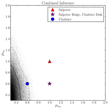
Figure 8: The IMF inferences obtained by naïve application of the single object model to all objects independently.

References

- Auger et al. (2010a) Auger, M. W., Treu, T., Bolton, A. S., et al. 2010a, ApJ, 724, 511
- Auger et al. (2010b) Auger, M. W., Treu, T., Gavazzi, R., et al. 2010b, ApJL, 721, L163
- Barnabè et al. (2013) Barnabè M., Spiniello C., Koopmans L. V. E., Trager S. C., Czoske O., Treu T., 2013, arXiv, arXiv:1306.2635
- Barnabè et al. (2012) Barnabè M., et al., 2012, MNRAS, 423, 1073
- Bastian, Covey, & Meyer (2010) Bastian N., Covey K. R., Meyer M. R., 2010, ARA&A, 48, 339
- Bell & de Jong (2001) Bell E. F., de Jong R. S., 2001, ApJ, 550, 212
- Bershady et al. (2011) Bershady, M. A., Martinsson, T. P. K., Verheijen, M. A. W., et al. 2011, ApJL, 739, L47
- Bolton et al. (2006) Bolton A. S., Burles S., Koopmans L. V. E., Treu T., Moustakas L. A., 2006, ApJ, 638, 703
- Cappellari et al. (2006) Cappellari M., et al., 2006, MNRAS, 366, 1126
- Cappellari et al. (2012) Cappellari M., et al., 2012, Natur, 484, 485
- Chabrier (2003) Chabrier, G. 2003, PASP, 115, 763
- Conroy & van Dokkum (2012) Conroy C., van Dokkum P., 2012, ApJ, 747, 69
- Dutton, Mendel, & Simard (2012) Dutton A. A., Mendel J. T., Simard L., 2012, MNRAS, L412
- Dutton et al. (2013) Dutton A. A., et al., 2013, MNRAS, 428, 3183
- Hogg, Myers, & Bovy (2010) Hogg D. W., Myers A. D., Bovy J., 2010, ApJ, 725, 2166
- Kelly (2007) Kelly B. C., 2007, ApJ, 665, 1489
- La Barbera et al. (2013) La Barbera F., Ferreras I., Vazdekis A., de la Rosa I. G., de Carvalho R. R., Trevisan M., Falcón-Barroso J., Ricciardelli E., 2013, arXiv, arXiv:1305.2273
- Loredo (2004) Loredo T. J., 2004, AIP Conference Series, 735, 195
- Loredo (2012) Loredo T. J., 2012, arXiv, arXiv:1208.3036
- Plummer (2003) Plummer, M., 2003, JAGS: A Program for Analysis of Bayesian Graphical Models Using Gibbs Sampling, Proceedings of the 3rd International Workshop on Distributed Statistical Computing (DSC 2003), March 20–22, Vienna, Austria. ISSN 1609-395X.
- Salpeter (1955) Salpeter E. E., 1955, ApJ, 121, 161
- Shu et al. (2012) Shu Y., Bolton A. S., Schlegel D. J., Dawson K. S., Wake D. A., Brownstein J. R., Brinkmann J., Weaver B. A., 2012, AJ, 143, 90
- Sonnenfeld et al. (2012) Sonnenfeld A., Treu T., Gavazzi R., Marshall P. J., Auger M. W., Suyu S. H., Koopmans L. V. E., Bolton A. S., 2012, ApJ, 752, 163
- Spiniello et al. (2012) Spiniello C., Trager S. C., Koopmans L. V. E., Chen Y. P., 2012, ApJ, 753, L32
- Tortora, Romanowsky, & Napolitano (2013) Tortora C., Romanowsky A. J., Napolitano N. R., 2013, ApJ, 765, 8
- Treu et al. (2010) Treu T., Auger M. W., Koopmans L. V. E., Gavazzi R., Marshall P. J., Bolton A. S., 2010, ApJ, 709, 1195
- Treu et al. (2011) Treu T., Dutton A. A., Auger M. W., Marshall P. J., Bolton A. S., Brewer B. J., Koo D. C., Koopmans L. V. E., 2011, MNRAS, 417, 1601 (Paper I)
- van Dokkum & Conroy (2010) van Dokkum P. G., Conroy C., 2010, Natur, 468, 940