A New Notion of Effective Resistance for Directed Graphs—Part II: Computing Resistances
Abstract
In Part I of this work we defined a generalization of the concept of effective resistance to directed graphs, and we explored some of the properties of this new definition. Here, we use the theory developed in Part I to compute effective resistances in some prototypical directed graphs. This exploration highlights cases where our notion of effective resistance for directed graphs behaves analogously to our experience from undirected graphs, as well as cases where it behaves in unexpected ways.
Index Terms:
Graph theory, networks, networked control systems, directed graphs, effective resistanceI Introduction
In the companion paper to this work, [1], we presented a generalization of the concept of effective resistance to directed graphs. This extension was constructed algebraically to preserve the relationships for directed graphs, as they exist in undirected graphs, between effective resistances and control-theoretic properties, including robustness of linear consensus to noise [2, 3], and node certainty in networks of stochastic decision-makers [4]. Further applications of this concept to directed graphs should be possible in formation control [5], distributed estimation [6, 7] and optimal leader selection in networked control systems [8, 9, 10].
Effective resistances have proved to be important in the study of networked systems because they relate global network properties to the individual connections between nodes, and they relate local network changes (e.g. the addition or deletion of an edge, or the change of an edge weight) to global properties without the need to re-compute these properties for the entire network (since only resistances that depend on the edge in question will change). Accordingly, the concept of effective resistance for directed graphs will be most useful if the resistance of any given connection within a graph can be computed, and if it is understood how to combine resistances from multiple connections. Computation and combination of resistances are possible for undirected graphs using the familiar rules for combining resistors in series and parallel.
In this paper, we address the problems of computing and combining effective resistances for directed graphs. In Section II we review our definition of effective resistance for directed graphs from [1]. In Section III we develop some theory to identify directed graphs that have the same resistances as an equivalent undirected graph. We use these results in Section IV to recover the series-resistance formula for nodes connected by one directed path and the parallel-resistance formula for nodes connected by two directed paths in the form of a directed cycle. In Section V we examine nodes connected by a directed tree and derive a resistance formula that has no analogue from undirected graphs.
II Background and notation
We present below some basic definitions of directed graph theory, as well as our definition of effective resistance. For more detail, the reader is referred to the companion paper [1].
A graph consists of the triple , where is the set of nodes, is the set of edges and is a weighted adjacency matrix with non-negative entries . Each will be positive if and only if , otherwise . The graph is said to be undirected if implies and . Thus, a graph will be undirected if and only if its adjacency matrix is symmetric.
The out-degree of node is defined as . has an associated Laplacian matrix , defined by , where is the diagonal matrix of node out-degrees.
A connection in between nodes and consists of two paths, one starting at and the other at and which both terminate at the same node. A direct connection between nodes and is a connection in which one path is trivial (i.e. either only node or only node ) - thus a direct connection is equivalent to a path. Conversely, an indirect connection is one in which the terminal node of the two paths is neither node nor node .
The graph is connected if it contains a globally reachable node. Equivalently, is connected if and only if a connection exists between any pair of nodes.
A connection subgraph between nodes and in the graph is a maximal connected subgraph of in which every node and edge form part of a connection between nodes and in . If only one connection subgraph exists in between nodes and , it is referred to as the connection subgraph and is denoted by .
Let be a matrix that satisfies
| (1) |
Using , we can compute the reduced Laplacian matrix for any graph as
| (2) |
and then for connected graphs we can find the unique solution to the Lyapunov equation
| (3) |
If we let
| (4) |
the resistance between two nodes in a graph can be computed as
| (5) |
Note that Definition LABEL:P1:def:generalres in the companion paper [1] extends effective resistance computations to disconnected graphs as well.
In some of the following results, we make use of binomial coefficients, defined as
| (6) |
III Directed and undirected graphs with equal effective resistances
In this section we prove Proposition 1, which provides sufficient conditions for the resistances in a directed graph to be the same as the resistances in an equivalent undirected graph. The proof relies on two lemmas, which we prove first.
Recall that a permutation matrix is a square matrix containing precisely one entry of in each row and column with every other entry being .
Lemma 1.
Let be a permutation matrix. Then has the following properties
-
(i)
-
(7)
-
-
(ii)
-
(8)
-
-
(iii)
-
(9)
-
Proof:
Since also satisfies the requirements of a permutation matrix, the results of Lemma 1 apply to as well (this can also be seen by simply transposing equations (i), (ii) and (iii)).
The following lemma is required to prove Proposition 1.
Lemma 2.
Let be a square matrix and be a permutation matrix of the same dimension as . Suppose that is diagonal. Then
-
(i)
is also diagonal,
-
(ii)
is symmetric, that is
(10) -
(iii)
-
(11)
-
Proof:
-
(i)
Let , which is diagonal by assumption. Then, by Lemma 1, we can see that . Thus , which implies that is formed by permuting the rows and columns of a diagonal matrix, and is therefore diagonal.
-
(ii)
Since and are diagonal, they are both symmetric. Thus () is symmetric too. Since is also symmetric, the result follows.
-
(iii)
First we note that as is diagonal, it is symmetric and commutes with its transpose (i.e. itself). Thus (by (i)). Similarly, by part (i), is also diagonal and so it too is symmetric and commutes with its transpose. Hence (by (i)). Using these facts, we can observe that . Now, adding to both sides gives us . But we can use (10) to write this as
(12) Now, by (iii), we can pre- or post-multiply any factor of or by without changing the matrix. Therefore, we can subtract from both sides of (12), obtain a common factor of on the left hand side and on the right hand side, then use (10) to obtain
which is equivalent to (using (iii) again)
Finally, pre-multiplying by and post-multiplying by gives us our desired result. ∎
The following proposition provides sufficient conditions for a directed graph to have the same resistances between any pair of nodes as an equivalent undirected graph. Although the assumption for the proposition may seem relatively general, it is straightforward to show that this can only apply to directed path and cycle graphs.
Proposition 1.
Suppose is a connected (directed) graph with matrix of node out-degrees . Furthermore, suppose there is a permutation matrix such that . Let be the undirected graph with , such that , and . Then the effective resistance between two nodes in is equal to the effective resistance between the same two nodes in .
Proof:
First we note that must be an undirected graph since its adjacency matrix is symmetric. The Laplacian matrix of is given by . Thus is given by , which can be rewritten (using (iii)) as . Furthermore, since is connected, is invertible [2].
Next, we claim that the Laplacian matrix of is given by . To see this, we first note that we can rewrite as . But by part (i) of Lemma 2, is diagonal and therefore so is . Hence is a diagonal matrix. Furthermore, . But since is a permutation matrix, and , and so . Therefore, is equal to a diagonal matrix minus and has zero row sums. Hence must be the diagonal matrix of the row sums of , i.e. the matrix of out-degrees of .
Since contains every edge in (in addition to the reversal of each edge) and is connected, must also be connected. Thus is the solution to the Lyapunov equation (3) for . Using our expression for and (iii), we can write . Since is symmetric, we can also write .
IV Effective resistances from direct connections
In this section we compute the resistance in directed graphs between a pair of nodes that are only connected through a single direct connection, or two direct connections in opposite directions (i.e. the connection subgraph consists of either a directed path or a directed cycle). These two scenarios are analogous (in undirected graphs) to combining multiple resistances in series and combining two resistances in parallel. At present, we do not have general rules for combining resistances from multiple direct connections.
The most basic connection is a single directed edge. Intuitively, since an undirected edge with a given weight is equivalent to two directed edges (in opposite directions) with the same weight, one would expect that the resistance of a directed edge should be twice that of an undirected edge with the same weight. The following lemma shows that this is indeed true.
Lemma 3.
If consists of a single directed edge from node to node with weight , then
| (14) |
Proof:
If we take node to be the first node in and node to be the second, then has Laplacian matrix . In this case, there is only one matrix (up to a choice of sign) which satisfies (1), namely . Then we have , and hence . Thus , and finally,
∎
As a result of Lemma 3, when we refer to the effective resistance of a single (directed) edge, we mean twice the inverse of the edge weight. Our next two results extend to some directed graphs the familiar rules from undirected graphs for combining resistances in series and parallel. These cover the cases when a pair of nodes is connected only by either a directed path or cycle.
Theorem 1.
Suppose consists of a single directed path. Then is given by the sum of the resistances of each edge in the path between the two nodes (where the resistance of each edge is computed as in Lemma 3).
Proof:
Suppose we label the nodes in from to in the order in which they appear along the path, starting with the root and moving in the direction opposite the edges. Then we can write the adjacency matrix of as , and the matrix of node out-degrees as .
If we let be the permutation matrix containing ones above the main diagonal and in the lower left corner, we can observe that . Therefore, by Proposition 1, the resistance between any two nodes in is equal to the resistance between the same two nodes in an undirected graph with adjacency matrix .
Now, is the adjacency matrix of an undirected path, with weights of on each edge. But the resistance of an edge in an undirected graph is the inverse of the edge weight and so each edge has resistance . Thus the edge resistances in this undirected graph match those in the original directed path graph (computed according to Lemma 3). Furthermore, the resistance between two nodes connected by an undirected path is simply the sum of the resistances of the edges between them. Thus the same is true for two nodes connected by a directed path. ∎
Theorem 2.
Suppose consists of a single directed cycle. Then is given by the inverse of the sum of the inverses of the resistances of each path connecting nodes and (where the resistance of each path is computed as in Theorem 1).
Proof:
Suppose we label the nodes in from to in the reverse of the order in which they appear around the cycle, starting with any node. Then we can write the adjacency matrix of as and the matrix of node out-degrees as .
If we let be the permutation matrix containing ones above the main diagonal and in the lower left corner, we can observe that . Therefore, by Proposition 1, the resistance between any two nodes in is equal to the resistance between the same two nodes in an undirected graph with adjacency matrix .
Now, is the adjacency matrix of an undirected cycle, with weights of on each edge. But the resistance of an edge in an undirected graph is the inverse of the edge weight, so each edge has resistance . Thus the edge resistances in this undirected graph match those in the original directed cycle graph (computed according to Lemma 3). Furthermore, the resistance between nodes and connected by an undirected cycle is given by
where is the resistance of one path between nodes and and is the resistance of the other path. Thus the same is true for two nodes connected by a directed cycle, where (by Theorem 1) and are equal to the resistances of the two directed paths between nodes and . ∎
V Effective resistances from indirect connections
Lemma 3 and Theorems 1 and 2 suggest a very intuitive interpretation of effective resistance for directed graphs. A directed edge can be thought of as “half” of an undirected edge - either by noting that a directed edge allows half of the interaction to take place that occurs through an undirected edge, or by viewing an undirected edge as consisting of two directed edges with equal weights but in opposite directions. Thus, the resistance of a directed edge is twice the resistance of an undirected edge with the same weight. Then, in path and cycle graphs, resistances combine in exactly the ways (i.e. in series and in parallel) we are used to. However, connections in directed graphs can be more complicated than these. In particular, two nodes in a directed graph may be connected even if neither node is reachable from the other. This will occur when the only connections between the nodes consist of two non-zero length paths which meet at a distinct node. In Theorem 3 we prove an explicit expression for resistances in the case when is a directed tree with unit edge weights. Before doing so we prove two lemmas on the correspondence between resistances and the matrix from (4), and two lemmas on the resistance between two leaves in a directed tree. We also rely on the finite series expressions given and proved in Appendix B.
Lemma 4.
There is a one-to-one relationship between the effective resistances between nodes in a graph and the entries of the matrix from (4). In particular,
| (15) |
| (16) |
Proof:
(15) is simply the definition of . To derive (16), we first note that from (1) and (4), has the property that and . That is, has zero row- and column-sums.
Lemma 5.
Suppose is a directed path with unit edge weights containing nodes, in which the nodes are labelled from to in the order in which they appear along the path, starting with the root. Let be the corresponding matrix from (4). Then the entries of are given by
| (19) |
Proof:
Suppose . Then by Theorem 1, we know that the resistance between nodes and in our directed path is equal to (the resistance of each edge) times the number of edges between them. Since the nodes are labelled in order along the path, this gives us . Therefore, from Lemma 4, we know that
| (20) |
We now proceed by examining each summation in turn. The first sum can be broken into two parts and then simplified using (i) to obtain . By replacing with in the previous expression, we observe that .
The following results are needed to prove Theorem 3. In them, we examine the resistance between the leaves of a tree containing two branches that meet at its root and with unit weights on every edge, , as shown in Fig. 1LABEL:sub@fig:C_G_n_m. The effective resistance between the two leaves of will be denoted by .
Lemma 6.
The effective resistance between the two leaves of is given by
| (21) |
Proof:
The number of nodes in is . Let us label the nodes in from to , in the reverse order of the edges, along the branch of length , starting with the root (thus the leaf of this branch is node ). Then the other leaf (with an edge connecting it to the root) will be node . Thus the resistance we seek to find is .
Let , and denote the adjacency matrix, matrix of out-degrees and Laplacian matrix of a directed path containing nodes and unit weights on every edge. Let the nodes in this path be labelled from to in the reverse of the order in which they appear, starting with the root. Thus , and . From these, we can observe that
| (22) |
| (23) |
Next, we will let be a matrix which satisfies (1), and and be derived from (2) and (3) using and . Let , according to (4). Then, by Lemma 5, the entries of are given by (19).
Now, we can write the adjacency matrix, matrix of out-degrees and Laplacian matrix of as , , and . Next, let , where and . Then satisfies (1). We can use (2), (22) and the facts that and to express as
In order to compute resistances in , we must find the matrix which solves (3). Since we have partitioned into a block matrix, we will do the same for . Let , where is a symmetric matrix, and . Then multiplying out the matrices in (3) and equating blocks in this matrix equation gives us
| (24) | ||||
| (25) | ||||
| (26) |
From (24), it is clear that . In addition, we can rewrite (26) as
| (27) |
In order to find a complete solution for , we must solve (25) for . However, resistances are computed from , which, if we let and use (4), can be written as
Hence, to compute resistances in , we need only compute , not . We can also note that as does not depend on our choice of (by Lemma LABEL:P1:lem:indofq in the companion paper [1]), neither does . In fact, we can write (27) as , and the resistance we seek as
| (28) |
Thus we only need to find and in order to compute .
Now, . We will therefore proceed by left-multiplying (25) by . Using the fact that , we obtain
| (29) |
But by (1), so by (22) and (23),
Furthermore, using (19), we observe that
Lemma 7.
For positive integers and , the resistance between the two leaves of satisfies the recurrence relation
| (35) |
The proof of Lemma 7 relies on similar ideas to the proof of Lemma 6, and is given in Appendix A. We now proceed to solve the recurrence relation given by Lemmas 6 and 7 using several finite series results given in Appendix B.
Theorem 3.
Suppose consists of a directed tree with unit weights on every edge. Then is given by
| (36) |
where is the length of the shortest path from node to a mutually reachable node and is the length of the shortest path from node to a mutually reachable node.
Proof:
Since every node in is reachable from either node or node , if is a tree then only nodes and can be leaves. But every tree has at least one leaf, so suppose that node is a leaf. If node is not a leaf, then must be a directed path and node is the closest mutually reachable node to both nodes and . Then , is the path length from to and (36) reduces to , which follows from Theorem 1. Conversely, if node is a leaf but node is not, must be a directed path and node is the closest mutually reachable node to both nodes and . Then , is the path length from to and (36) reduces to . But by (iv) and (ii) from Lemma 10, , and so (36) becomes , which follows from Theorem 1.
Now, if both node and node are leaves, then must be a directed tree with exactly two branches. Thus must correspond to the tree shown in Fig. 1LABEL:sub@fig:C_G_tree and and are the path lengths from nodes and , respectively, to the point where the two branches meet. Furthermore, both and are at least .
By Corollary LABEL:P1:cor:removepath from the companion paper [1], we observe that the resistance between nodes and remains the same as we remove all the nodes of from the root to the node where the two branches meet. Thus, can be computed as the resistance between the two leaves of the tree shown in Fig. 1LABEL:sub@fig:C_G_n_m. Let this tree be called , and since the only two parameters that define are and , we can write as a function of and only. That is,
(a)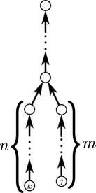
(b)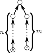
In order to compute , we will begin by considering the case where . Substituting into (36) gives , which follows from Lemma 6.
Now, suppose that (36) holds for all and all (for some ). Then for can be computed using Lemma 7. In particular, all resistances in the right-hand side of (35) are given by (36). Therefore, we find that matches the expression given in Lemma 15. Therefore, can be expressed in the form given in (96).
Next, suppose that is odd. That is, for some integer . Then (96) gives us
| (37) |
where is given by (86) in Lemma 13. But by Lemma 13, for any integers and . Thus (36) holds for .
Finally, suppose that is even. That is, for some integer . Then (96) gives us
where is given by (95) in Lemma 14. But by Lemma 14, for any integers and . Thus,
and so (36) holds for .
Therefore, by induction we have that (36) also holds for all and . ∎
Equation (36) is a highly non-intuitive result, not least because on initial inspection it does not appear to be symmetric in and (although we know that it must be, by Theorem LABEL:P1:theo:metric in the companion paper). Therefore, it becomes easier to interpret (36) if we reformulate it in terms of the shorter path length and the difference between the path lengths. Thus, if we let be the length of the longer path, that is, for some , (36) becomes
Then, using (6), we can write
and hence conclude that . Thus, when the connection subgraph between two nodes is a directed tree, the resistance between them is twice the difference between the lengths of the paths connecting each node to their closest mutually reachable node, plus some “excess” that disappears as this difference becomes large. Conversely, the excess is significant when the path length difference is small, leading to a resistance that is greater than twice the difference.
One common approach to the analysis of resistive circuits is to replace a section of the network that connects to the rest through a single pair of nodes by a single resistor with an equivalent resistance. The simplest example of this is the replacement of a path with a single edge with equivalent resistance. If this principle were to extend to the calculation of effective resistance in directed graphs, then in (as shown in Fig. 2) would match the formula from Theorem 3. However, a simple calculation shows that in ,
which only matches (36) for . Thus in more general cases of connection subgraphs like but with arbitrary weights on every edge, the resistance between the leaves does not depend only on the equivalent resistance of each path.

Theorems 1, 2 and 3 by no means characterise all the possible connection subgraphs in a directed graph. Other connection subgraphs include multiple paths from to (some of which could coincide over part of their length), multiple paths from to and multiple paths from to (again, some of which could partially coincide), multiple indirect connections of the type analysed in Theorem 3 (which could partially coincide) and a combination of indirect and direct (i.e. path) connections. Further analysis is needed to completely describe how to compute resistances in these situations.
VI Conclusions
The results of Lemma 3 and Theorems 1 and 2 demonstrate that in some situations our definition of effective resistance for directed graphs behaves as an intuitive extension of effective resistance in undirected graphs. In contrast, Theorem 3 demonstrates a fundamental difference between effective resistance in directed and undirected graphs that arises from the fundamentally different connections that are possible only in directed graphs. Nevertheless, the results presented above show that our notion of effective resistance for directed graphs provides an approach that can relate the local structure of a directed graph to its global properties. The familiar properties of effective resistance allows for a firm analysis of directed graphs that behave similarly to undirected graphs, while the unfamiliar properties can provide insight for the design of directed networks which contain essential differences as compared to undirected networks.
Appendix A Proof of Lemma 7
Proof:
As stated in the lemma, we will assume that and are positive integers throughout this proof. Let be the number of nodes in . The branch of length contains nodes (excluding the root), while the other branch contains nodes (excluding the root). Therefore, we have . Let us label the nodes in from to along the branch of length , in reverse order of the edge directions and starting with the root (thus the leaf of this branch is node ). Then let us label the nodes in the branch of length from to in reverse order of the edge directions. Thus the second leaf is node .
In the following, we will denote the adjacency matrix of by , its matrix of node out-degrees by and its Laplacian matrix by . Furthermore, we will let be a matrix that satisfies (1) and and be the corresponding matrices from (2) and (3) using and . Finally, will be the matrix from (4), computed using and . Then, by Lemma 4, the entries of are related to the resistances in by (16).
As in the proof of Lemma 6, let , and denote the adjacency matrix, matrix of out-degrees and Laplacian matrix of a directed path containing nodes and unit weights on every edge. Let the nodes in this path be labelled from to in the order in which they appear, starting with the root. Then we can write , and in terms of , and as follows: , and .
Let us now consider . By our labeling convention, the resistance between the two leaves of is given by . Now, we can write the adjacency matrix of in terms of as . In a similar fashion, we can write the matrix of node out-degrees for as , and the Laplacian matrix as .
Now, let , where and . Then satisfies (1). We can therefore use (2), (38) and the facts that and to compute as
In order to compute resistances in , we must find the matrix which solves (3). Since we have partitioned into a block matrix, we will do the same for . Let , where is a symmetric matrix, and . Then multiplying out the matrices in (3) and equating blocks in this matrix equation gives us
| (40) | ||||
| (41) | ||||
| (42) |
From (40), it is clear that . In addition, we can rewrite (42) as
| (43) |
Thus in order to find a complete solution for , we must solve (41) for . However, resistances are computed from the entries of , which, if we let and use (4), can be written as
Hence, in order to compute resistances in , we need only compute , not . We should also note that as does not depend on our choice of (by Lemma LABEL:P1:lem:indofq in the companion paper [1]), neither does . In fact, we can write (43) as , and the resistance we seek as
| (44) |
Thus we only need to find , and in order to compute .
Now, . We will therefore proceed by left-multiplying (41) by . Using the fact that , we obtain
| (45) |
But by (1), and so by using (38) and (39), we find
Furthermore, we observe that , , and .
Substituting these expressions into (45) gives us
| (46) | ||||
| (47) | ||||
| (48) |
Similarly, we can recursively apply (46) times, starting with , substitute in (47) and simplify using (iii) to find
| (50) |
But now (48), (49) and (50) form a set of three of simultaneous linear equations in , and . Substituting their solution into (44) and then multiplying by (and using the definitions of and ) gives us
| (51) |
Now, by (5), we can write . Furthermore, by Theorem 1 we know that
| (52) |
| (53) |
Finally, by the definition of , we can say that
| (54) |
Therefore, we can substitute for each non-diagonal term in (51) and use (iii) and (iv), along with the fact that to find
or, by changing indices inside the sums,
| (55) |
Appendix B Finite series
The following series are either well-known or special cases of well-known series. The first two and the general cases of the third and fourth usually appear in any introductory mathematical text that covers series (e.g. section 4.2 of [13]). The fifth is slightly more obscure.
Lemma 8.
For integer values of ,
-
(i)
-
(59)
-
-
(ii)
-
(60)
-
-
(iii)
-
(61)
-
-
(iv)
-
(62)
-
-
(v)
-
(63)
-
Proof:
B-A Finite series of binomial coefficients
Although there are many interpretations and uses of binomial coefficients, we will simply assume two basic facts about them, namely Pascal’s rule;
| (64) |
and the binomial formula;
| (65) |
Pascal’s rule follows easily from (6) while the binomial formula can be inductively proved using Pascal’s rule. Equations (64) and (65) can also be found in standard introductory mathematics texts, such as sections 1.5–1.6 in [13].
We can use Pascal’s rule to derive some identities involving binomial coefficients. These identities include the two in the following lemma.
Lemma 9.
For integer values of and , with , and ,
-
(i)
-
(66)
-
-
(ii)
-
(67)
-
Proof:
Both results can be easily proven using mathematical induction and Pascal’s rule. ∎
A special case of the binomial formula can be found by substituting into (65), which gives
| (68) |
Differentiating this expression with respect to gives us
| (69) |
In the following results, we will make use of a few “well-known” series of binomial coefficients (for example, the first two can be found in Chapter 3 of [15] and all can be solved by Mathematica). Since they are not as standard as the basic facts stated above, we will include a brief proof of them for the sake of completeness.
Lemma 10 (Standard sums of binomial coefficients).
For integer values of ,
-
(i)
-
(70)
-
-
(ii)
-
(71)
-
-
(iii)
-
(72)
-
-
(iv)
-
(73)
-
Proof:
Substituting into (68) gives us and for any . Equations (i) and (ii) can be found by taking the sum and difference of these two expressions and dividing by . Similarly, substituting into (69) gives us and for any . Equations (iii) and (iv) can be found by taking the sum and difference of these two expressions and dividing by . ∎
We can now use the results from Lemma 10 to derive some more specialised series. These are summarised in the following lemma. As a point of notation, we will assume that any sum not containing any terms (such as ) is equal to zero.
Lemma 11 (Specialised sums of binomial coefficients).
For integer values of ,
-
(i)
-
(74)
-
-
(ii)
-
(75)
-
-
(iii)
-
(76)
-
-
(iv)
-
(77)
-
-
(v)
-
(78)
-
-
(vi)
-
(79)
-
-
(vii)
-
(80)
-
-
(viii)
-
(81)
-
Proof:
In addition to these series evaluations, the following series manipulations will prove to be useful.
Lemma 12 (Equivalent binomial series).
For integer values of and ,
-
(i)
-
(82)
and
-
-
(ii)
-
(83)
-
Proof:
-
(i)
First, let us suppose that , and is an integer between and (inclusive). Then, we can use Pascal’s rule with to write , while for we can say . With these two facts, we can write
(84) By shifting indices by , substituting in (84), and then rearranging, the first sum on the right becomes
and so (84) becomes
Substituting this expression into the left hand side of (i) produces the desired result.
-
(ii)
Again, let us suppose that , and is an integer, now between and (inclusive). As above, we can use Pascal’s rule to write
(85) By shifting indices by , substituting in (85), and then rearranging, the first sum on the right becomes
and so (85) becomes
Substituting this expression into the left hand side of (ii) produces the desired result. ∎
Now, we can use Lemmas 11 and 12 to evaluate two more complicated expressions which will be necessary for the completion of our derivation.
Lemma 13.
Let and be non-negative integers, and let
| (86) |
Then .
Proof:
First, we can use (iii) to simplify the third term in the first sum. In addition, the third term in the second sum can be written as using Pascal’s rule for . We can then apply (viii) to the term. This gives us
| (87) |
Next, we will consider the case when . Using (6) and (iii), we can simplify to find that . Thus, in the rest of the proof, we will assume that . Furthermore, when , we can use (i), (iii) and (viii) to find that .
Next, let us consider . Substituting in for in (87), taking the terms out of the final sum and applying (64) and (i) gives us
| (88) |
Now, let us define a new function, , as
| (89) |
Then, from (87) and (88), we obtain
| (90) |
We can use (i), (iii) and (viii) to show that . In a similar manner as before, we will next consider . Substituting in for in (90), taking the terms out of the final sum and applying (64) and (i) produces
| (91) |
Once again, we will define a new function, , as
| (92) |
Note that is well-defined since its denominator is positive for all and . Then, from (90) and (91), we obtain
| (93) |
Using (iii) and (viii), we find that . Finally, we will follow our previous procedure once more and consider . Substituting in for in (93), using (64) and (i), and comparing to (93) produces
| (94) |
Hence, from (94) and , we conclude that . Substituting this result into (92) tells us that , which, along with the fact that , allows us to conclude that .
Finally, we can substitute this result into (89) to find that
which, along with the facts that and , gives us our desired result. ∎
Lemma 14.
Let and be non-negative integers, and let
| (95) |
Then .
Proof:
This proof proceeds almost exactly as the proof of Lemma 13. The only differences are that we use (64), (iv), (v), (vi) and (ii) to simplify expressions (rather than (iii), (64), (i), (iii), (viii) and (i)) and our intermediate functions are defined as
where is well-defined since its denominator is positive for all and . ∎
Our final result covers some simplification required for the proof of Theorem 3.
Lemma 15.
Suppose and are positive integers, and let
,
,
,
,
, and
.
Then
| (96) |
References
- [1] G. Young, L. Scardovi, and N. Leonard, “A new notion of effective resistance for directed graphs—Part I: Definition and properties,” 2013, submitted to IEEE Trans. Autom. Control.
- [2] ——, “Robustness of noisy consensus dynamics with directed communication,” in Proc. ACC, Baltimore, MD, 2010, pp. 6312–6317.
- [3] ——, “Rearranging trees for robust consensus,” in Proc. CDC-ECC, Orlando, FL, 2011, pp. 1000–1005.
- [4] I. Poulakakis, L. Scardovi, and N. Leonard, “Node classification in networks of stochastic evidence accumulators,” 2012, arXiv:1210.4235 [cs.SY].
- [5] P. Barooah and J. Hespanha, “Graph effective resistance and distributed control: Spectral properties and applications,” in Proc. CDC, San Diego, CA, 2006, pp. 3479–3485.
- [6] ——, “Estimation on graphs from relative measurements,” IEEE Control Syst. Mag., vol. 27, no. 4, pp. 57–74, 2007.
- [7] ——, “Estimation from relative measurements: Electrical analogy and large graphs,” IEEE Trans. Signal Process., vol. 56, no. 6, pp. 2181–2193, 2008.
- [8] S. Patterson and B. Bamieh, “Leader selection for optimal network coherence,” in Proc. CDC, Atlanta, GA, 2010, pp. 2692–2697.
- [9] A. Clark and R. Poovendran, “A submodular optimization framework for leader selection in linear multi-agent systems,” in Proc. CDC-ECC, Orlando, FL, 2011, pp. 3614–3621.
- [10] M. Fardad, F. Lin, and M. Jovanovic̀, “Algorithms for leader selection in large dynamical networks: Noise-free leaders,” in Proc. CDC-ECC, Orlando, FL, 2011, pp. 7188–7193.
- [11] R. Horn and C. Johnson, Matrix Analysis. New York, NY: Cambridge University Press, 1985.
- [12] M. Woodbury, Inverting modified matrices, ser. Memorandum Report no. 42, Statistical Research Group. Princeton, NJ: Princeton University, 1950.
- [13] K. Riley, M. Hobson, and S. Bence, Mathematical Methods for Physics and Engineering, 3rd ed. New York, NY: Cambridge University Press, 2006.
- [14] E. Hansen, A table of series and products. Englewood Cliffs, NJ: Prentice-Hall, 1975.
- [15] M. Spiegel, S. Lipschutz, and J. Liu, Mathematical Handbook of Formulas and Tables, 3rd ed. New York, NY: McGraw-Hill, 2009.