Antiscreening of the Ampère force in QED and QCD plasmas

Abstract

The static forces between electric charges and currents are modified at the loop level by the presence of a plasma. While electric charges are screened, currents are not. The effective coupling constant at long distances is enhanced in both cases as compared to the vacuum, and by different amounts, a clear sign that Lorentz symmetry is broken. We investigate these effects quantitatively, first in a QED plasma and secondly using non-perturbative simulations of QCD with two light degenerate flavors of quarks.

I Introduction

The properties of Abelian and non-Abelian plasmas are the subject of intensive experimental and theoretical investigation. See Arnold et al. (2012) for a recent overview of the status of research on the quark-gluon plasma, and Thoma (2009) for a comparative discussion of Abelian and non-Abelian plasmas. Electromagnetic probes play an important role in heavy ion collision experiments, see for instance the recent Gale (2012); Shen et al. (2013). In particular, it is important to understand the way in which electromagnetic interactions are modified by the presence of a thermal medium. While calculating dynamical properties Brandt et al. (2013); Ding et al. (2011); Amato et al. (2013); Ghiglieri et al. (2013) is crucial to predicting experimental observables in heavy-ion collisions, here we will concentrate on static (time-independent) aspects of the electromagnetic force in a plasma.

It is well-known that the electric force is screened by the quasi-free charges of a plasma. This phenomenon of Debye screening occurs already in a plasma described by classical physics. The static force between currents however remains unscreened. The coupling constants of both forces are in fact enhanced at long distances as compared to the vacuum. In the vacuum, the intensity of the Coulomb force and the Ampère force are related, a consequence of Lorentz symmetry Purcell (1963). In a medium such as a plasma, they may have a different intensity. They receive a factor $(1+e^{2}\kappa_{\ell})$ and $(1+e^{2}\kappa_{t})$ respectively, where both $\kappa_{\ell}$ and $\kappa_{t}$ are found to be positive and $\kappa_{\ell}>\kappa_{t}$. These coefficients are determined by the long-wavelength behavior of the static polarization tensor. An important point is that since the renormalized electromagnetic coupling is defined conventionally at long distances in the vacuum state (zero temperature), it is necessary to subtract the vacuum polarization tensor in order to obtain the medium-induced modification of the long-range force between renormalized charges and currents.

The enhancement of the effective coupling constant is perhaps physically more relevant in the case of currents, since the Ampère force remains unscreened. The enhancement of the latter can be understood intuitively, by noting that free charges that happen to be moving parallel to the external current line are attracted to it, thus reinforcing it, while free charges moving antiparallel are repelled. It is thus fair to speak of a medium-induced ‘antiscreening’ of the Ampère force. This picture is corroborated by the fact that the quantity $\kappa_{t}$, which quantifies the enhancement of the force, also enters the constitutive equation of the electric current at second order in a ‘hydrodynamic’ description, $\boldsymbol{j}=e\kappa_{t}\nabla\times\boldsymbol{B}\,+$ other terms Hong and Teaney (2010).

As a potential QED application, consider the early universe in its first few minutes. There is a period where electrons and positrons, which are still relativistic, dominate the energy density along with photons, with comparatively few nucleons present. The protons can then be considered as slow-moving probes of the relativistic QED plasma. They interact at long distances via a Debye-screened potential. Its coefficient is modified by a factor $(1+e^{2}\kappa_{\ell})$. Note, however, that at the same order one also has to consider the two-photon exchange amplitude.

A coefficient analogous to $\kappa_{t}$ has been introduced in the constitutive equation of shear stress Baier et al. (2008), where it is denoted by $\kappa$. It multiplies a term that vanishes in flat space. It has been computed in the SU($N$) gauge theory at weak coupling in leading order Romatschke and Son (2009) and has recently been addressed non-perturbatively using lattice Monte-Carlo simulations Philipsen and Schaefer (2013).

After deriving the physics interpretation of $\kappa_{\ell}$ and $\kappa_{t}$, we recall the known one-loop formulae for the polarization function in QED and extract the quantities $\kappa_{\ell}$ and $\kappa_{t}$ (section II). The QCD case is simply obtained by multiplying the results by the number of colors carried by the quarks. In section III we then proceed to calculate for the first time the polarization function in the deconfined phase of QCD. We use Monte-Carlo simulations of lattice QCD with two flavors of quarks (with the O($a$) improved Wilson action).

II Theory

In this section we define the correlation functions relevant to the calculation of the coefficients $\kappa_{\ell}$ and $\kappa_{t}$. We give their interpretation in subsection II.2. In subsection II.3, we review the role of $\kappa_{t}$ as a second order coefficient in the constitutive equation of the electromagnetic current. Finally, we review the one-loop results for the polarization tensor and extract analytic representations for $\kappa_{\ell}$ and $\kappa_{t}$ useful at small and at large fermion masses.

II.1 Definitions

We work in the Euclidean field theory. The vector current is defined as $j_{\mu}(x)=\bar{\psi}(x)\gamma_{\mu}\psi(x)$, where the Dirac matrices are all hermitian and satisfy $\{\gamma_{\mu},\gamma_{\nu}\}=2\delta_{\mu\nu}$. We define the polarization tensor as

$$\Pi_{\mu\nu}(q)\equiv\int d^{4}x\,e^{iq\cdot x}\langle j_{\mu}(x)j_{\nu}(0)\rangle.$$ (1)

In the vacuum, it is purely transverse,

$$\Pi^{\rm vac}_{\mu\nu}(q) = P_{\mu\nu}(q)q^{2}\Pi^{\rm vac}(q^{2}),$$ (2)

$$P_{\mu\nu}(q) = q_{\mu}q_{\nu}/q^{2}-\delta_{\mu\nu}.$$ (3)

With these conventions, the spectral function

$$\rho^{\rm vac}(s)\equiv-2\;{\rm Im}\,\Pi^{\rm vac}(-s-i\epsilon)\qquad(s\geq 0)$$ (4)

is non-negative for a flavor-diagonal correlator. For the electromagnetic current, it is related to the $R$ ratio via

$$\rho^{\rm vac}(s)=\frac{R(s)}{6\pi},\qquad R(s)\equiv\frac{\sigma(e^{+}e^{-}\to{\rm hadrons})}{4\pi\alpha(s)^{2}/(3s)}.$$ (5)

The denominator is the treelevel cross-section $\sigma(e^{+}e^{-}\to\mu^{+}\mu^{-})$ in the limit $s\gg m_{\mu}^{2}$, and we have neglected QED corrections.

At finite temperature $T\equiv 1/\beta$, the tensor decomposition reads

$$\Pi_{\mu\nu}(q)=P^{L}_{\mu\nu}(q)\,\Pi_{L}(q_{0}^{2},\boldsymbol{q}^{2})+P^{T}_{\mu\nu}(q)\,\Pi_{T}(q_{0}^{2},\boldsymbol{q}^{2}),$$ (6)

where $P^{T}_{00}(q)=0=P^{T}_{0i}(q)=P^{T}_{i0}(q)$ and $P^{T}_{ij}(q)=q_{i}q_{j}/\boldsymbol{q}^{2}-\delta_{ij}$, while $P^{L}_{\mu\nu}(q)=P_{\mu\nu}(q)-P^{T}_{\mu\nu}(q)$.

We define the ‘matter’ part of the polarization tensor via

$$\Pi_{\mu\nu}(q) \equiv \Pi^{\rm vac}_{\mu\nu}(q)+\Pi_{\mu\nu}^{\rm mat}(q),$$ (7)

$$\Pi_{L}^{\rm mat}(q) \equiv \Pi_{L}(q)-q^{2}\Pi^{\rm vac}(q^{2}),$$ (8)

$$\Pi_{T}^{\rm mat}(q) \equiv \Pi_{T}(q)-q^{2}\Pi^{\rm vac}(q^{2}).$$ (9)

With these conventions, following Hong and Teaney (2010) we define

$$\kappa_{t} = -\left.\frac{\partial}{\partial(q_{3}^{2})}\Pi_{11}^{\rm mat}(q_{3}\boldsymbol{e}_{3})\right|_{q_{3}=0}=\left.\frac{\partial}{\partial(\boldsymbol{q}^{2})}\Pi^{\rm mat}_{T}(0,\boldsymbol{q}^{2})\right|_{\boldsymbol{q}=0},$$ (10)

$$\kappa_{\ell} = -\left.\frac{\partial}{\partial(q_{3}^{2})}\Pi_{00}^{\rm mat}(q_{3}\boldsymbol{e}_{3})\right|_{q_{3}=0}=\left.\frac{\partial}{\partial(\boldsymbol{q}^{2})}\Pi^{\rm mat}_{L}(0,\boldsymbol{q}^{2})\right|_{\boldsymbol{q}=0}.$$ (11)

We now turn to the interpretation of these quantities.

II.2 Interpretation of $\kappa_{\ell}$ and $\kappa_{t}$

Consider an $SU(3)\times U(1)$ vector gauge theory with quarks as the only matter fields. Let $S$ be the action of quarks (described by the field $\psi(x)$), gluons ($A_{\mu}(x)$) and photons ($B_{\mu}(x)$). The partition function of the system coupled to a classical electromagnetic source $J_{\mu}(x)$ (it satisfies $\partial_{\mu}J_{\mu}(x)=0$) reads

$$Z[J]=\int D[\bar{\psi}]D[\psi]\,D[A]\,D[B]\;\exp\left(-S-ie_{0}\int d^{4}x\;B_{\mu}(x)J_{\mu}(x)\right).$$ (12)

Expanding the free energy $F[J]=-\frac{1}{\beta}\log Z[J]$ in $J$, one obtains for the quadratic term

$$F^{(2)}[J]=\frac{e_{0}^{2}}{2\beta}\int d^{4}x\int d^{4}y\;\langle B_{\mu}(x)B_{\nu}(y)\rangle_{J=0}\;J_{\mu}(x)J_{\nu}(y).$$ (13)

II.2.1 Free energy of electromagnetic sources at zero-temperature

Consider first the situation at zero temperature. In one loop approximation in the electromagnetic coupling $e$, the photon propagator is such that

$$\int d^{4}x\;J_{\mu}(x)\;\langle B_{\mu}(x)B_{\nu}(y)\rangle_{J=0}=\int d^{4}x\;J_{\mu}(x)\;\int\frac{d^{4}q}{(2\pi)^{4}}\;\frac{\delta_{\mu\nu}~{}e^{iq(x-y)}}{q^{2}(1-e_{0}^{2}\Pi^{\rm vac}(q^{2}))}.$$ (14)

For a static source of the form

$$J_{0}(x)=Q_{1}\delta^{(3)}(\boldsymbol{x})+Q_{2}\delta^{(3)}(\boldsymbol{x}-\boldsymbol{r}),\qquad\qquad J_{i}(x)=0,$$ (15)

$F^{(2)}[J]$ can be interpreted as the static potential between two static U(1) charges. As a check that one recovers the familiar expression, for the source (15) the quadratic contribution to the free energy becomes

$$F^{(2)}(r)=V(r)=Q_{1}Q_{2}\int\frac{d^{3}\boldsymbol{q}}{(2\pi)^{3}}\;\frac{e_{0}^{2}}{1-e_{0}^{2}\Pi^{\rm vac}(\boldsymbol{q}^{2})}\frac{e^{i\boldsymbol{q}\cdot\boldsymbol{r}}}{\boldsymbol{q}^{2}}+\dots$$ (16)

where the remaining terms are independent of $\boldsymbol{r}$. The renormalization of the electric charge leads to the substitution

$$\frac{e_{0}^{2}}{1-e_{0}^{2}\Pi^{\rm vac}(\boldsymbol{q}^{2})}=\frac{e^{2}}{1-e^{2}[\Pi^{\rm vac}(\boldsymbol{q}^{2})-\Pi^{\rm vac}(0)]}$$ (17)

at one-loop accuracy. We have thus recovered the familiar expression of the Coulomb potential, modified by the vacuum polarization Weinberg (1995), the so-called Uehling potential.

II.2.2 Generalization to finite temperature

In momentum space, the $(00)$ component of the static (i.e. $q_{0}=0$) photon propagator is given at one loop by

$$\int d^{4}x\;e^{-i\boldsymbol{q}(\boldsymbol{x}-\boldsymbol{y})}\;\langle B_{0}(x)B_{0}(y)\rangle_{J=0}=\frac{1}{\boldsymbol{q}^{2}-e_{0}^{2}\Pi_{L}(0,\boldsymbol{q}^{2})}.$$ (18)

Since the electric charge is conventionally renormalized at zero temperature, the free energy added by the presence of the two static leptons is given by

$$F_{l}^{(2)}(r) = Q_{1}Q_{2}\int\frac{d^{3}\boldsymbol{q}}{(2\pi)^{3}}\;\frac{e_{0}^{2}}{\boldsymbol{q}^{2}-e_{0}^{2}\Pi_{L}(0,\boldsymbol{q}^{2})}\;e^{i\boldsymbol{q}\cdot\boldsymbol{r}}$$ (19)

$$= Q_{1}Q_{2}\int\frac{d^{3}\boldsymbol{q}}{(2\pi)^{3}}\;\frac{e^{2}}{1-e^{2}[\Pi^{\rm mat}_{L}(0,\boldsymbol{q}^{2})/\boldsymbol{q}^{2}+\Pi^{\rm vac}(\boldsymbol{q}^{2})-\Pi^{\rm vac}(0)]}\;\frac{e^{i\boldsymbol{q}\cdot\boldsymbol{r}}}{\boldsymbol{q}^{2}}.$$ (20)

Given the expansion at small momenta

$$\Pi^{\rm mat}_{L}(0,\boldsymbol{q}^{2})=-\chi_{s}+\kappa_{l}\boldsymbol{q}^{2}+\dots,$$ (21)

and $\Pi^{\rm vac}(\boldsymbol{q}^{2})-\Pi^{\rm vac}(0)={\rm O}(\boldsymbol{q}^{2})$, the Coulomb potential is screened at long distances, with a screening mass given by

$$m_{\rm el}^{2}=e^{2}\chi_{s}.$$ (22)

Explicitly, the interaction free energy is given at long distances by

$$F_{l}^{(2)}(r)=\frac{e^{2}}{1-e^{2}\kappa_{l}}\;\frac{Q_{1}Q_{2}\,e^{-m_{\rm el}r}}{4\pi r}.$$ (23)

Consider now the stationary source

$$iJ_{3}(x)=I_{1}\delta^{(2)}(\boldsymbol{x}_{\perp})+I_{2}\delta^{(2)}(\boldsymbol{x}_{\perp}+\boldsymbol{R}_{\perp}),\qquad\boldsymbol{x}_{\perp}\equiv(x_{1},x_{2}),$$ (24)

where the other components of $J_{\mu}$ vanish. It describes two long wires along the $\boldsymbol{e}_{3}$ direction (which we take to be length $L_{3}$), separated by a distance $|\boldsymbol{R}_{\perp}|$. The currents $I_{1}$ and $I_{2}$ correspond to the charge, measured in units of $e$, that flows per unit time along the $\boldsymbol{e}_{3}$ direction. Then, up to $|\boldsymbol{R}_{\perp}|$-independent terms,

$$F_{t}^{(2)}(R_{\perp}) = -I_{1}I_{2}L_{3}\int\frac{d^{2}\boldsymbol{q}_{\perp}}{(2\pi)^{2}}\;\frac{e_{0}^{2}}{\boldsymbol{q}_{\perp}^{2}-e_{0}^{2}\Pi_{T}(\boldsymbol{q}_{\perp}^{2})}\;e^{i\boldsymbol{q}_{\perp}\cdot\boldsymbol{R}_{\perp}}$$ (25)

$$= -I_{1}I_{2}L_{3}\int\frac{d^{2}\boldsymbol{q}_{\perp}}{(2\pi)^{2}}\;\frac{e^{2}}{1-e^{2}[\Pi^{\rm mat}_{T}(\boldsymbol{q}_{\perp}^{2})/\boldsymbol{q}_{\perp}^{2}+\Pi^{\rm vac}(\boldsymbol{q}_{\perp}^{2})-\Pi^{\rm vac}(0)]}\;\frac{e^{i\boldsymbol{q}_{\perp}\cdot\boldsymbol{R}_{\perp}}}{\boldsymbol{q}_{\perp}^{2}}$$ (26)

Thus we see that the transverse channel $\Pi_{T}$ modifies Ampère’s $1/R_{\perp}$ force law. At long distances, the modification is given by

$$-\frac{1}{L_{3}}\frac{\partial F_{t}^{(2)}}{\partial R_{\perp}}=-\frac{e^{2}}{1-e^{2}\kappa_{t}}\cdot\frac{I_{1}I_{2}}{2\pi R_{\perp}}.$$ (27)

Thus a positive value of $\kappa_{t}$ corresponds to an enhancement of the strength of the $1/R_{\perp}$ force law, as compared to the Ampère force in the vacuum.

II.3 Constitutive equation of the electromagnetic current

The equation of continuity for the electric charge, $\dot{\rho}+\nabla\cdot\boldsymbol{j}=0$, can be used to describe the time evolution of a non-equilibrium initial charge distribution. This ‘hydrodynamic’ description applies on long distance and time scales. It needs to be supplemented by a constitutive equation in order to be predictive. At lowest order in a derivative expansion, $e\boldsymbol{j}=\sigma\boldsymbol{E}-eD\nabla\rho$, with the conductivity $\sigma$ and the diffusion coefficient related by $\sigma=\chi_{s}D$. At the next order, the most general allowed terms are of the form Hong and Teaney (2010)

$$(1+\tau_{J}\partial_{t})e\boldsymbol{j}=-eD\nabla\rho+\sigma\boldsymbol{E}+\kappa_{B}\nabla\times\boldsymbol{B}.$$ (28)

Note that in our conventions, for the QCD plasma $\sigma$ and $\kappa_{B}$ are both of order $e^{2}$ in the electromagnetic coupling. Through the linear response formalism, one shows Hong and Teaney (2010) that the coefficient multiplying the the curl of $\boldsymbol{B}$ is directly related to the quantity $\kappa_{t}=\kappa_{B}/e^{2}$ introduced above from the medium-induced part of the polarization function $\Pi_{T}^{\rm mat}$.

Equation (28) confirms the interpretation that the coefficient $\kappa_{t}>0$ corresponds to an antiscreening of electric currents in the medium. Indeed, suppose an external current $I_{0}=I_{\rm ext}$ flowing along a straight line is applied to the system, creating circular magnetic field lines around it. If we choose a transverse disc $S$ (with an edge $\partial S$) centered on it, the response electric current $e\int_{S}d\sigma\cdot\boldsymbol{j}$ flowing through $S$ is given by $I_{1}=\kappa_{B}\int_{\partial S}d\boldsymbol{\ell}\cdot\boldsymbol{B}$. This current enhances the circulation of the magnetic field along $\partial S$ by an amount equal to $I_{1}$, which in turn induces a current $I_{2}$. This amounts to a geometric series $\sum_{k=0}^{\infty}I_{k}$, so that the net effect is to enhance $I_{0}$ by a factor $1/(1-\kappa_{B})$.

II.4 Leading-order perturbative results

We now give one-loop results for the polarization tensor and its small $\boldsymbol{q}^{2}$ expansion in a pure QED plasma with one Dirac fermion of mass $m$ carrying a charge $e$. The expressions for QCD are obtained by summing the contribution of each quark flavor and multiplying the result by the number of colors $N_{c}$.

In QED at leading order, the vacuum polarization reads (see for instance Weinberg (1995))

$$\Pi^{\rm vac}(q^{2})-\Pi^{\rm vac}(0) = \frac{1}{2\pi^{2}}\int_{0}^{1}dx\,x(1-x)\log\left[1+\frac{q^{2}x(1-x)}{m^{2}}\right].$$ (29)

Two independent components of the thermal contribution read Kapusta and Gale (2006), with $E_{\boldsymbol{k}}=\sqrt{\boldsymbol{k}^{2}+m^{2}}$ and $n_{F}(E)=1/(e^{\beta E}+1)$,

$$\Pi_{00}^{\rm mat}(q) = \frac{2}{\pi^{2}}{\rm Re}\int_{0}^{\infty}{k^{2}dk}\,\frac{n_{F}(E_{\boldsymbol{k}})}{E_{\boldsymbol{k}}}\left[1+\frac{4E_{\boldsymbol{k}}^{2}-4iE_{\boldsymbol{k}}q_{0}-q_{0}^{2}-\boldsymbol{q}^{2}}{4k|\boldsymbol{q}|}\,\log\frac{R_{+}}{R_{-}}\right],$$ (30)

$$\Pi^{\rm mat}_{\mu\mu}(q) = \frac{4}{\pi^{2}}{\rm Re}\int_{0}^{\infty}k^{2}dk\,\frac{n_{F}(E_{\boldsymbol{k}})}{E_{\boldsymbol{k}}}\left[1+\frac{2m^{2}-q_{0}^{2}-\boldsymbol{q}^{2}}{4|\boldsymbol{q}|k}\log\frac{R_{+}}{R_{-}}\right],$$

$$R_{\pm} = {q_{0}^{2}+\boldsymbol{q}^{2}\pm 2|\boldsymbol{q}|k+2iq_{0}E_{\boldsymbol{k}}}.$$ (31)

From here one obtains the longitudinal and transverse part of the polarization tensor via

$$\Pi_{L}(q_{0}^{2},\boldsymbol{q}^{2})=-\Pi_{00}(q),\qquad\qquad\Pi_{T}(q_{0}^{2},\boldsymbol{q}^{2})=\frac{1}{2}\left(\Pi_{00}(q)-\Pi_{\mu\mu}(q)\right).$$ (32)

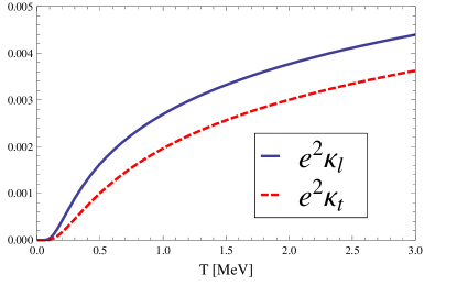
Figure 1: The coefficients $e^{2}\kappa_{\ell}$ and $e^{2}\kappa_{t}$ at one loop in QED, with the fermion mass set to $m_{e}=0.511{\rm MeV}$ and $e^{2}=4\pi/137$.

The expression for the fermion number susceptibility reads

$$\Pi_{00}^{\rm mat}(q=0)=-\Pi_{L}(0,0)=-\Pi^{\rm mat}_{L}(0,0)=\chi_{s}=\frac{2}{\pi^{2}}\int_{0}^{\infty}\frac{dk}{E_{\boldsymbol{k}}}\,n_{F}(E_{\boldsymbol{k}})\;(k^{2}+E_{\boldsymbol{k}}^{2})=-\frac{2m^{2}}{\pi^{2}}\sum_{n\geq 1}(-1)^{n}\;K_{2}(n\,\beta m).$$ (33)

In the massless limit, we have $\chi_{s}=T^{2}/3$.

In the transverse channel, we obtain from (30–II.4)

$$\kappa_{t}=\frac{1}{3\pi^{2}}\int_{0}^{\infty}\frac{dk}{E_{\boldsymbol{k}}}\;n_{F}(E_{\boldsymbol{k}})=-\frac{1}{3\pi^{2}}\sum_{n=1}^{\infty}(-1)^{n}\,K_{0}(n\,\beta m).$$ (34)

For small $\beta m$, we find the expansion (see appendix A)

$$\kappa_{t}=\frac{1}{6\pi^{2}}\left(\log\left({1}/{b}\right)-\gamma_{\rm E}\right)+{\rm O}(b^{2}\log(1/b)),\qquad b\equiv\frac{m}{\pi T}.$$ (35)

There is an infrared divergence coming from the $T=0$ contribution. In QCD, this divergence is driven by the light pions rather than by the light quarks, but the infrared sensitivity is also present.

It is convenient to consider the difference $\kappa_{\ell}-\kappa_{t}$, since it is infrared safe, unlike $\kappa_{\ell}$ and $\kappa_{t}$ individually. We find

$$\kappa_{\ell}-\kappa_{t}=-\frac{1}{6\pi^{2}}\int_{0}^{\infty}dp\;n_{F}^{\prime}(E_{\boldsymbol{p}})=-\frac{\beta m}{6\pi^{2}}\sum_{n=1}^{\infty}(-1)^{n}\,n\,K_{1}(n\,\beta m),$$ (36)

where $n_{F}^{\prime}(E)\equiv\frac{dn_{F}}{dE}$. At small $\beta m$, its expansion is

$$\kappa_{\ell}-\kappa_{t}=\frac{1}{12\pi^{2}}\left(1-{\frac{7}{4}}\zeta_{3}\,b^{2}+{\frac{93}{32}}\zeta_{5}\,b^{4}+{\rm O}(b^{6})\right),$$ (37)

and it would not be difficult to extend the series to higher orders. Note that $\kappa_{\ell}-\kappa_{t}$ amounts to a small number compared to the fermionic contribution to the entropy, $s/T^{3}=7\pi^{2}/45$ in the massless case.

Finally, as a numerical application, we display the value of the coefficients $\kappa_{\ell}$ and $\kappa_{t}$ in QED as a function of the temperature in Fig. 1. If we think about the early universe, we note that around the time when free neutrons start to disappear by $\beta$ decay ($T\simeq 0.8{\rm MeV}$, see for instance the recent review Olive (2012)), $\kappa_{\ell}$ and $\kappa_{t}$ represent a 2–3 permille effect on the inter-proton electromagnetic force. By the time the nucleosynthesis chain starts (around $T=0.1{\rm MeV}$), the effect really is tiny.

If we now consider the quark-gluon plasma, we expect the difference $\kappa_{\ell}-\kappa_{t}$ to be well described by the leading perturbative formulae above (with the suitable $N_{c}$ and $N_{f}$ factors) at sufficiently high temperature, since it is not infrared-sensitive at leading order in perturbation theory. The value of the individual coefficients $\kappa_{\ell}$ and $\kappa_{t}$ however emerge from an interesting interplay between ultraviolet and infrared physics. Indeed, without the vacuum subtraction, they would be ultraviolet divergent, but on the other hand, the vacuum contribution is infrared divergent for massless fermions. In QCD, this infrared contribution is non-perturbative (it is dominated by pions), and therefore we turn to lattice simulations in order to evaluate $\kappa_{\ell}$ and $\kappa_{t}$ individually.

III Numerics

Figure 2: The PCAC quark masses in the $x_{3}$ direction as calculated on our finite temperature lattice ensemble of size $16\times 64^{3}$. See the text for details on obtaining the quoted values $m/T$.

In this section, we describe a numerical lattice QCD calculation of the antiscreening coefficients $\kappa_{l}$ and $\kappa_{t}$, as well as of the free energy of two static leptons for a general separation $r$.

All our numerical results were obtained on dynamical gauge configurations with two mass-degenerate quark flavors. The gauge action is the standard Wilson plaquette action Wilson (1974), while the fermions were implemented via the O($a$) improved Wilson discretization with non-perturbatively determined clover coefficient $c_{\rm sw}$ Jansen and Sommer (1998). The configurations were generated using the MP-HMC algorithm Hasenbusch (2001); Hasenbusch and Jansen (2003) in the implementation of Marinkovic and Schaefer Marinkovic and Schaefer (2010) based on Lüscher’s DD-HMC package CLS (2010a).

We calculated correlation functions using the same discretization and masses as in the sea sector on two lattice ensembles. One at zero temperature and a lattice of size $128\times 64^{3}$ (labeled O7 in Fritzsch et al. (2012)) with a lattice spacing of $a=0.0486(4)(5)$fm Fritzsch et al. (2012) and a pion mass of $m_{\pi}=270$MeV, so that $m_{\pi}L=4.2$. The second at finite temperature with a lattice of size $16\times 64^{3}$ with all bare parameters identical to the zero-temperature ensemble. The zero-temperature ensemble was made available to us through the CLS effort CLS (2010b), while the second ensemble was generated by us and already presented in Brandt et al. (2013). Note that choosing $N_{\tau}=16$ yields a temperature of $T\simeq 250$MeV. Based on preliminary results on the pseudo-critical temperature $T_{c}$ of the crossover from the hadronic to the high-temperature phase Brandt et al. (2012), the temperature can also be expressed as $T/T_{c}\approx 1.2$.

In addition we calculated correlation functions on the same ensembles with the bare quark mass tuned to match the physical strange quark mass Capitani et al. (2011). More precisely, the bare quark mass is fixed at zero temperature by tuning the kaon mass to the value realized in nature. According to perturbation theory, the most relevant dimensionless parameter is $m/T$. In order to facilitate a comparison with the one-loop results, we therefore measure this quantity directly using the partially conserved axial current (PCAC) relation Bochicchio et al. (1985); Luscher et al. (1997) in the finite-temperature ensemble. Since it is an operator identity, we are free to evaluate the correlation functions of the axial current and the pseudoscalar density in the longer spatial direction to evaluate the quark mass. Specifically, we define

$$m_{\rm AWI}(x_{3})=\frac{1}{2}\sum_{(x_{0},x_{1},x_{2})}\frac{\langle\partial^{\rm imp}_{3}J^{I}_{3,5}(x)J_{5}(0)\rangle}{\langle J_{5}(x_{i})J_{5}(0)\rangle}\quad,$$ (38)

where $J_{5}(x_{i})$ and $J^{I}_{\mu,5}(x_{i})=J_{\mu,5}(x_{i})+ac_{A}\partial^{\rm imp}_{\mu}J_{5}(x_{i})$ denote the (isovector) pseudoscalar density and improved axial-vector current, respectively. As ‘improved’ lattice derivatives $\partial^{\rm imp}_{\mu}$ we use the higher-order difference scheme given in Guagnelli et al. (2001), Eq. (2.18–2.19). Here, for the improvement coefficient $c_{A}$ we use the non-perturbatively determined value of Della Morte et al. (2005a). The extraction of the PCAC mass is illustrated in Fig. 2. The quoted values for $m/T$ were determined by fitting a constant to $m_{\rm AWI}(x_{3})$ over the interval indicated by the band in Fig. 2. The result was found to be stable under variations of the fit interval. To renormalize the PCAC quark mass we use the non-perturbatively determined renormalization factors $Z_{A}$ and $Z_{P}$ of the axial current and the pseudoscalar density of Fritzsch et al. (2012); Della Morte et al. (2009), as well as the conversion factor from the Schrödinger functional scheme to the $\overline{\rm MS}$ scheme from Della Morte et al. (2005b); Fritzsch et al. (2012). Altogether the factor by which we multiply the bare PCAC mass to obtain the $\overline{\rm MS}$ mass at a renormalization scale of $\mu=2\,$GeV is $1.481(34)$. The result as well as all relevant parameters are collected in Tab. 1. From now on we simply refer to these $\overline{\rm MS}$ quark masses by $m$.

$6/g_{0}^{2}$	5.50
$\kappa$	0.13671
$c_{SW}$	1.751496
$m_{\pi}$[MeV]	270
$Z_{V}$	0.768(5)
$a[\textrm{fm}]$	0.0486(4)(5)
$T_{N_{\tau}=16}$[MeV]	253(4)
$\overline{m}_{\rm ud}^{\overline{\rm MS}}(2\,{\rm GeV})/T$	0.0325(48)(7)
$\overline{m}_{\rm s}^{\overline{\rm MS}}(2\,{\rm GeV})/T$	0.3747(30)(86)

Table 1: The top block shows the bare lattice parameters, for more details on the $N_{\tau}=128$ and $N_{\tau}=16$ ensembles see Fritzsch et al. (2012); Brandt et al. (2013, 2012). The middle block summarizes the pion mass, the vector renormalization constant Della Morte et al. (2005c), the lattice spacing Fritzsch et al. (2012) and the corresponding temperature of our $N_{\tau}=16$ lattice calculation. In the bottom block we give the renormalized quark masses in units of temperature, where the first error is from the bare axial Ward identity mass and the second from the renormalization factor.

We implemented the vector correlation function as a mixed correlator between the local and the conserved current. In the following we will require the three correlation functions:

$$G^{\rm bare}(x_{0},g_{0},T)\,\delta_{kl} =-a^{3}\sum_{(x_{1},x_{2},x_{3})}\langle J^{c}_{k}(x)J^{l}_{\ell}(0)\rangle,\quad k,l=1,2,3,$$ (39)

$$G_{t}^{\rm bare}(x_{3},g_{0},T)\,\delta_{ij} =-a^{3}\sum_{(x_{0},x_{1},x_{2})}\langle J^{c}_{i}(x)J^{\ell}_{j}(0)\rangle,\quad i,j=1,2,$$ (40)

$$G_{l}^{\rm bare}(x_{3},g_{0},T) =-a^{3}\sum_{(x_{0},x_{1},x_{2})}\langle J^{c}_{0}(x)J^{\ell}_{0}(0)\rangle,$$ (41)

where

$$J_{\mu}^{l}(x) = \frac{1}{\sqrt{2}}\bar{q}(x)\gamma_{\mu}{\tau^{3}}q(x),$$ (42)

$$J_{\mu}^{c}(x) = \frac{1}{2\sqrt{2}}\Big{(}\bar{q}(x+a\hat{\mu})(1+\gamma_{\mu})U_{\mu}^{\dagger}(x){\tau^{3}}q(x)-\bar{q}(x)(1-\gamma_{\mu})U_{\mu}(x){\tau^{3}}q(x+a\hat{\mu})\Big{)}.$$ (43)

Here $q$ represents a doublet of mass-degenerate quark fields and $\tau^{3}$ the diagonal Pauli matrix acting on the flavor indices. The doublet can be interpreted as the (u, d) quarks (which are treated fully dynamically) for the light mass case, while it can be interpreted as a ‘partially quenched’ (s, s^′) doublet for the heavier case (i.e. their back-reaction on the thermal system is neglected). We note that with this normalization of the current, the perturbative prediction for its two-point function is given by $N_{c}=3$ times the expressions given in section II.4.

We have renormalized the vector correlator using

$$G_{..}(x_{i},T)=Z_{V}(g_{0})\;G_{..}^{\rm bare}(x_{i},g_{0},T)$$ (44)

with the non-perturbative value of $Z_{V}=0.768(5)$ Della Morte et al. (2005c). We have not included O($a$) contributions from the improvement term proportional to the derivative of the antisymmetric tensor operator Luescher et al. (1996); Sint and Weisz (1997). A quark-mass dependent improvement term of the form $(1+b_{V}(g_{0})am_{q})$ Sint and Weisz (1997) was also neglected. These contributions should eventually be included to ensure a smooth scaling behavior as the continuum limit is taken. Here, our primary goal is to carry out the analysis on a single lattice spacing.

III.1 Correlator data and screening masses

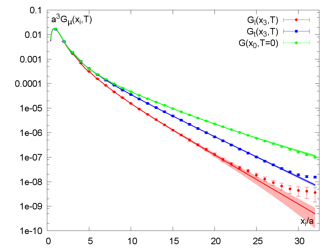
Figure 3: Local-conserved vector correlation functions for the light quarks (left panel) and the strange quark (right panel). The shaded bands represent the correlators entering the computation of the antiscreening coefficients and the free energy.

Reaching our goal of computing the antiscreening coefficients and the free energy requires the computation of three vector correlation functions: the vector correlator at zero temperature (Eq. 39) in the $x_{0}$ direction, as well as the individual transverse (Eq. 40) and longitudinal (Eq. 41) vector correlators in the $x_{3}$-direction.

To treat the latter required integrals over the spatial vector correlation functions without introducing unnecessarily large finite lattice effects, we employ the position space representation introduced in Francis et al. (2013). Here, the local-conserved correlator was extrapolated with an exponential that decays with the lowest-lying ‘mass’ . This mass can be fixed by fitting to the lattice data an Ansatz of the form

$$G_{\rm Ansatz}(x_{i})=\sum_{n=1}^{2}|A_{n}|^{2}e^{-m_{n}x_{i}},$$ (45)

for $x_{i}$ sufficiently below the half-lattice extent $N_{i}/2$ that the ‘backward’ propagating states give a negligible contribution. In the zero temperature ensemble this mass can be determined reliably by extracting it from a separate correlation function, computed on the same configurations using smeared operators at the source and sink Francis et al. (2013); Capitani et al. (2011). This operator has greater overlap with the ground state and yields more precise data. The mass parameter determined in this way is then carried over to the local-conserved correlator and the corresponding prefactor of the exponential $|A_{1}|^{2}$ is fitted to the lattice data around $x_{0}=\beta/4$. For the finite temperature ensembles, we did not compute vector correlation functions using smeared-smeared operators but fitted using the local-conserved data directly. However, due to the better signal-to-noise ratio in the finite temperature case, accurate results can nevertheless be obtained in this fashion.

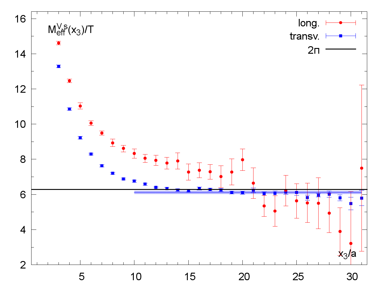
Figure 4: The effective screening masses (defined by Eq. (46)) for the longitudinal and the transverse channels. The left panel corresponds to the light quark case and the right panel to the strange quark. The band shows the result of the fit for the mass with its statistical error.

The raw lattice data as well as the resulting correlation functions are shown as the colored shaded bands in Fig. 3, where the error estimates were obtained via a jackknife procedure. For the light-quark longitudinal correlator, the relative errors grow rapidly for $x_{3}/a\gtrsim 20$, but this has little impact on our determination of the antiscreening coefficients and the free energy of two static leptons.

As a byproduct of our study, we can investigate the lowest-lying screening masses coupling to the isovector vector current. For that purpose, in Fig. 4 we display the effective screening masses, defined by the implicit equation

$$\frac{G(x_{3}-a/2)}{G(x_{3}+a/2)}=\frac{\cosh\big{[}M_{\rm eff}^{V}(x_{3})({L}/{2}-(x_{3}-a/2))\big{]}}{\cosh\big{[}M_{\rm eff}^{V}(x_{3})({L}/{2}-(x_{3}+a/2))\big{]}}.$$ (46)

This form corrects for the leading effects of the finite length of the $x_{3}$ direction. In the transverse channel, we observe a convincing plateau, showing that we observe the asymptotic screening mass. In the longitudinal channel, the correlator initially falls off with a substantially higher exponent, but at distances beyond $x_{3}\approx\beta$, the effective exponent appears to decrease to a value below $2\pi T$. A possible interpretation is that the charge density operator couples only weakly to the lightest state in that channel, and therefore initially decays with a higher exponent. Given this behavior, we leave the extraction of a screening mass in the longitudinal channel for a future study with increased statistics and possibly improved spectroscopic methods. In the transverse channel, we extract the following values for the screening mass,

$$\frac{M^{V}_{t}}{2\pi T}=\left\{\begin{array}[]{l@{~~~~}l}0.943(17)\hfil~{}~{}~{}~{}&\textrm{light quarks}\\ 0.973(21)\hfil~{}~{}~{}~{}&\textrm{strange quarks}.\end{array}\right.$$ (47)

The quoted error contains an estimate of the uncertainty associated with choosing a fit interval. We thus have rather convincing evidence that the screening mass lies below $2\pi T$ for light quarks. These results can be compared to the perturbative prediction $M_{t}^{V}/(2\pi T)=1+0.02980g^{2}$ for two massless flavors of quarks Laine and Vepsalainen (2004). Presumably the value of the screening mass reaches values above $2\pi T$ at sufficiently high temperatures. Interestingly, the charge density operator (corresponding to the longitudinal channel) also plays a somewhat special role in the perturbative analysis Laine and Vepsalainen (2004). It would be worth revisiting this special case. In addition to the masses, the coupling $|A_{1}|^{2}$ of the lightest screening state to the vector current is of significant interest. In the regime where the hierarchy $gT\ll\pi T$ applies, it is proportional to the wavefunction at the origin describing the bound state of two fermions effectively of mass $\pi T$. We find, in the transverse channel,

$$\frac{1}{T^{3}}|A_{1}|^{2}=\left\{\begin{array}[]{l@{~~~~}l}6.05\pm 0.78\hfil~{}~{}~{}~{}&\textrm{light quarks}\\ 5.80\pm 1.10\hfil~{}~{}~{}~{}&\textrm{strange quarks}.\end{array}\right.$$ (48)

A future comparison with perturbative calculations would be complementary to the comparison of the screening masses.

III.2 The antiscreening coefficients $\kappa_{t}$, $\kappa_{l}$ and $(\kappa_{l}-\kappa_{t})$

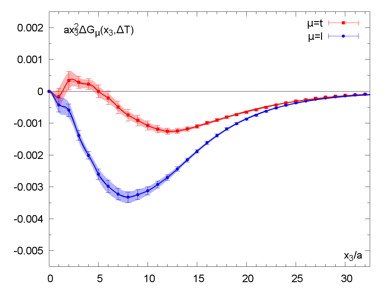
Figure 5: The integrands $x_{3}^{2}\,\Delta G_{\mu}(x_{3},T)$ for the convolution integrals of Eq. (49) and Eq. (50) for the light quark mass $m_{\rm ud}$ in the left panel and the strange quark mass $m_{\rm s}$ in the right panel.

In order to obtain $\kappa_{t}$, $\kappa_{l}$ and $(\kappa_{l}-\kappa_{t})$ given the local-conserved correlation functions of Fig. 3, one has to compute the following integrals:

$$\kappa_{t} =-\int_{0}^{\infty}dx\,x^{2}\,\Delta G_{t}(x,T), \Delta G_{t}(x,T)\equiv G_{t}(x,T)-G(x,0),$$ (49)

$$\kappa_{l} =-\int_{0}^{\infty}dx\,x^{2}\,\Delta G_{l}(x,T), \Delta G_{l}(x,T)\equiv G_{l}(x,T)-G(x,0),$$ (50)

$$\kappa_{l}-\kappa_{t} =-\int_{0}^{\infty}dx\,x^{2}\,\Delta G_{l-t}(x,T), \Delta G_{l-t}(x,T)\equiv G_{l}(x,T)-G_{t}(x,T).$$ (51)

To compute these integrals, we employ the parametrized correlation functions of Fig. 3, form the relevant differences, multiply the latter by $x^{2}$ and integrate them. The integrands for $\kappa_{t}$ and $\kappa_{l}$ in the light quark case are shown in the left panel of Fig. 5, while the corresponding strange quark results are given in the right panel. At large distances, $x_{3}\gtrsim 2/T$, the integrand is strongly suppressed. At the same time, the explicit factor $x_{3}^{2}$ induces an exact zero at $x_{3}=0$ in the integrand. For the longitudinal case a broad peak in the negative $y$-direction emerges with a minimum at $x_{3}\simeq(2T)^{-1}$. In the transverse case the integrand first yields positive results before passing through zero and also exhibiting a negative peak shape. Both results depend strongly on the mass value, as the light-quark curve drops roughly a factor 1.5–2.0 lower than the strange-quark curve.

The integral is carried out using standard numerical integration techniques (for example the ‘global adaptive’ strategy using the ‘Gauss-Kronrod rule’ or ‘trapezoidal rule’ options supplied by the Mathematica-package work very well here) for a set of jackknife bins, yielding a central value and an error estimate. We obtain, for the two quark masses,

$$\kappa_{t}(m_{\rm ud})=0.0400(39) ,\quad\quad\quad\kappa_{t}(m_{\rm s})=0.0169(17)\,,$$ (52)

$$\kappa_{l}(m_{\rm ud})=0.0750(34) ,\quad\quad\quad\kappa_{l}(m_{\rm s})=0.0458(19)\,.$$ (53)

These values are similar to the corresponding one-loop QED predictions for $m/T\simeq 1$ (if one divides the former by the $N_{c}=3$ factor). This reflects the fact that the infrared behavior of the vector correlator in QCD is very different from its QED counterpart due to confinement and chiral symmetry breaking. In QED, a substantial fermion mass mimicks to a certain extent the rapid fall-off of the QCD correlator.

Figure 6: The integrand $x_{3}^{2}\,\Delta G_{l-t}(x_{3},T)$ of Eq. (51) for the light and the strange quark cases. The corresponding quantity for free massless fermions is displayed as a black curve.

Since the zero temperature correlator drops out in $(\kappa_{l}-\kappa_{t})$, the latter difference is determined more accurately. The corresponding integrand for both masses is shown in Fig. 6, where we also give the one-loop lattice result (computed in appendix B) for comparison. For both values of the quark mass we observe a broad peak in the negative direction. While qualitatively similar, the non-perturbative data falls off somewhat more slowly than the one-loop result, in spite of the fact that the quark mass is finite in the simulation and set to zero in the one-loop curve. The resulting values of the integrals are:

$$(\kappa_{l}-\kappa_{t})(m_{\rm ud})=0.0350(24) ,\quad\quad\quad(\kappa_{l}-\kappa_{t})(m_{\rm s})=0.0290(21)\,.$$ (54)

Due to the slower fall-off of the screening correlators observed in the data, the value of this difference is noticibly larger than the one-loop calculation predicts,

$$\qquad\qquad(\kappa_{l}-\kappa_{t})_{m/T=0.033}=0.0253 ,\quad\quad\quad(\kappa_{l}-\kappa_{t})_{m/T=0.38}=0.0246\,\qquad\quad(\textrm{one loop}),$$ (55)

particularly for the light quark mass case. It would be interesting to see whether a two-loop calculation could account for the discrepancy.

III.3 Implications for the free energy of two static leptons in the quark-gluon plasma

To compute the free energy of two static electric charges in a QCD plasma in the one-photon exchange approximation, it is useful to switch to a position-space representation of the one-loop correction to the static photon propagator. The reason is that the integral over the module of the spatial momentum in Eq. (20) is not absolutely convergent. Defining $\tilde{j}_{\mu}(x_{3})\equiv\int dx_{0}dx_{1}dx_{2}j_{\mu}(x)$, the representation

$$F_{l}^{(2)}(r,T) = \frac{Q_{1}Q_{2}e^{2}\,e^{-m_{\rm el}r}}{4\pi r}\Big{(}1+e^{2}h_{l}(r,T)\Big{)},$$ (56)

$$h_{l}(r,T) = \int_{0}^{\infty}dx_{3}\,\left(\phi_{\ell}(r,x_{3})\,\Big{\langle}\tilde{j}_{0}(x_{3})j_{0}(0)\Big{\rangle}_{T}-x_{3}^{2}\,\Big{\langle}\tilde{j}_{0}(x_{3})j_{0}(0)\Big{\rangle}_{0}\right),$$ (57)

$$\phi_{\ell}(r,x_{3}) = \left\{\begin{array}[]{l@{\qquad}l}x_{3}^{2}&x_{3}<r,\\ 2x_{3}r-r^{2}&x_{3}\geq r,\end{array}\right.$$ (60)

is equivalent, up to higher order terms in the coupling $e$, to Eq. (20). However, the integral over $x_{3}$ to be performed numerically is now exponentially convergent for all $r$ in the infrared, and the integrand is finite around $x_{3}=0$. Moreover, since we identified the exponential fall-off of the correlator at long distances, this representation is less affected by the finite box length $L_{3}$ used in the simulation Francis et al. (2013) than the momentum space representation.

We recall that in the continuum, the two integrals contributing to $h_{l}$ taken separately are logarithmically divergent in the ultraviolet, but that their difference is finite. On the lattice, the corresponding sums are of course separately finite. For large $r$, $h_{l}(r,T)$ tends to $\kappa_{l}$. For small $r$, the thermal correlator can be approximated by the vacuum correlator and one recovers from Eq. (56) the standard expression for the potential $V(\boldsymbol{r})$ modified by vacuum polarization effects, the so-called Uehling potential (see for instance Weinberg (1995)).

Similarly, in the case of two stationary, parallel currents, the negative derivative of the free energy reads

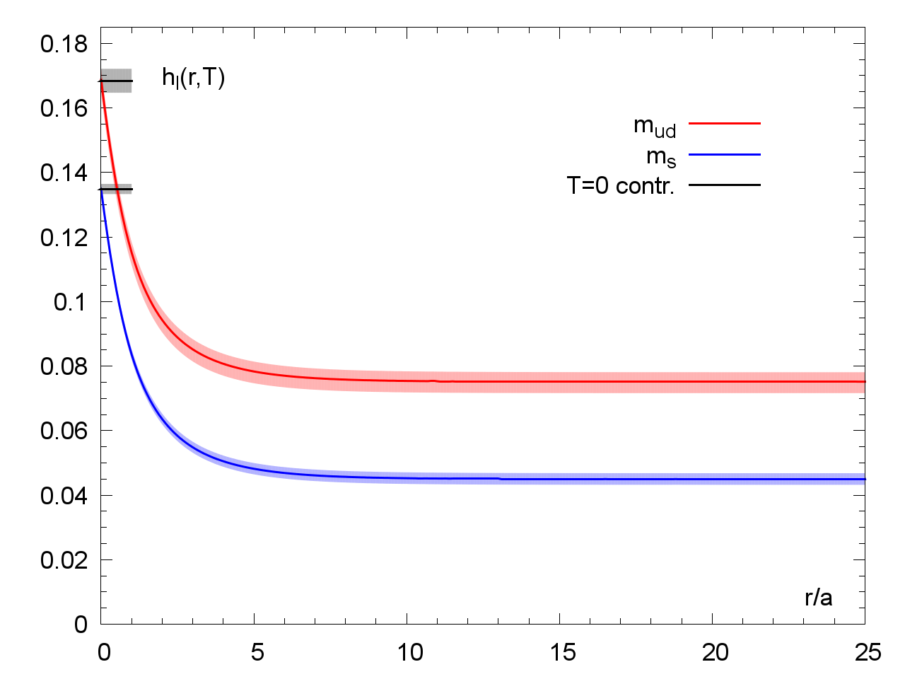
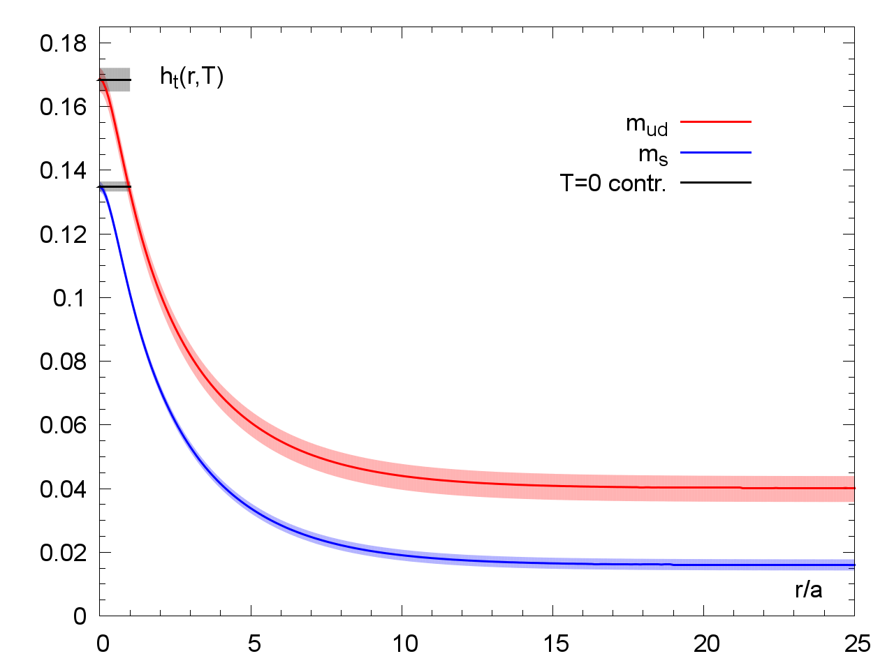
Figure 7: The modification terms of the free energy of two static charges in a QED plasma. Left: $h_{l}(r,T)$ of Eq. (56). Right: $h_{t}(r,T)$ of Eq. (61). In both cases the light and strange quark results are displayed respectively in red and blue. We highlight the $r$-independent $T=0$ contribution in black around $r=0$.

$$-\frac{1}{L_{3}}\frac{\partial}{\partial r}F_{t}^{(2)}(r,T)\! = \!-\frac{I_{1}I_{2}e^{2}}{2\pi r}\Big{(}1+e^{2}h_{t}(r,T)\Big{)},$$ (61)

$$h_{t}(r,T) = \int_{0}^{\infty}\!dx_{3}\,\left(\phi_{t}(r,x_{3})\,\Big{\langle}\tilde{j}_{1}(x_{3})j_{1}(0)\Big{\rangle}_{T}-x_{3}^{2}\,\Big{\langle}\tilde{j}_{1}(x_{3})j_{1}(0)\Big{\rangle}_{0}\right),$$ (62)

$$\phi_{t}(r,x_{3}) = \left\{\begin{array}[]{l@{\qquad}l}x_{3}^{2}&x_{3}<r,\\ x_{3}^{2}-x_{3}\sqrt{x_{3}^{2}-r^{2}}-r^{2}\log\frac{r}{x_{3}+\sqrt{x_{3}^{2}-r^{2}}}&x_{3}\geq r.\end{array}\right.$$ (65)

These equations allow us to compute the generalization of the electric Ampère force for currents immersed in hot, strongly interacting matter.

Now the integrals in Eq. (56) and Eq. (61) are of the same form as those of Eqs. (49–51) and to compute these loop corrections we may reuse the machinery developed to calculate the antiscreening coefficients. The results for both correction functions are shown in Fig. 7, where the red and blue lines denote the light and strange quark mass cases, respectively. We give the distance $r$ in lattice units and highlight the $r$-independent $T=0$ contribution by short black bands around $r=0$ (again, this contribution is logarithmically divergent in the continuum limit). In both cases we observe a sharp drop from the $T=0$ contribution at small $r$ with the results leveling off to a constant. In the case of the free energy of two static leptons in the left panel of Fig. 7, the dependence on $r$ rapidly becomes negligible; it levels off into a constant shift to the leading order term at around $r/a\simeq 10$. At this point the results for the two masses differ by roughly a factor 1.5. In the case of the derivative of the free energy of two parallel currents, the distance dependence quickly becomes negligible and levels off around $r/a\simeq 20$. In this case the mass dependence is seen to give roughly a factor 2 between the light and strange quark cases. Comparing the errors from the $T=0$ contribution and the respective $T\neq 0$ parts, we note that the $T=0$ uncertainty dominates at large distances. In the limit $r\rightarrow\infty$ the terms $h_{l}(r,T)$ and $h_{t}(r,T)$ become equivalent to those of Eq. (49) and Eq. (50), which provides a useful cross-check of our calculations and indeed the results agree as expected.

To illustrate the difference of this result with the zero-temperature case, we display the hadronic vacuum polarization contribution to the electric potential between two electric charges in Fig. 8. In the limit $T\to 0$, Eq. (56) simplifies to

$$V(r) = \frac{Q_{1}Q_{2}e^{2}}{4\pi r}\Big{(}1+e^{2}h_{l}(r,0)\Big{)},$$ (66)

$$h_{l}(r,0) = -\int_{r}^{\infty}dx_{3}\;(r-x_{3})^{2}\;\langle\tilde{j}_{0}(x_{3})\,j_{0}(0)\rangle_{0}\,.$$ (67)

In particular, the relative correction $h(r,0)$ to the Coulomb potential is positive definite, i.e. the effective QED coupling becomes stronger at short distances, as expected. Unlike in the thermal case, the correction goes to zero rapidly beyond a distance of 1fm.

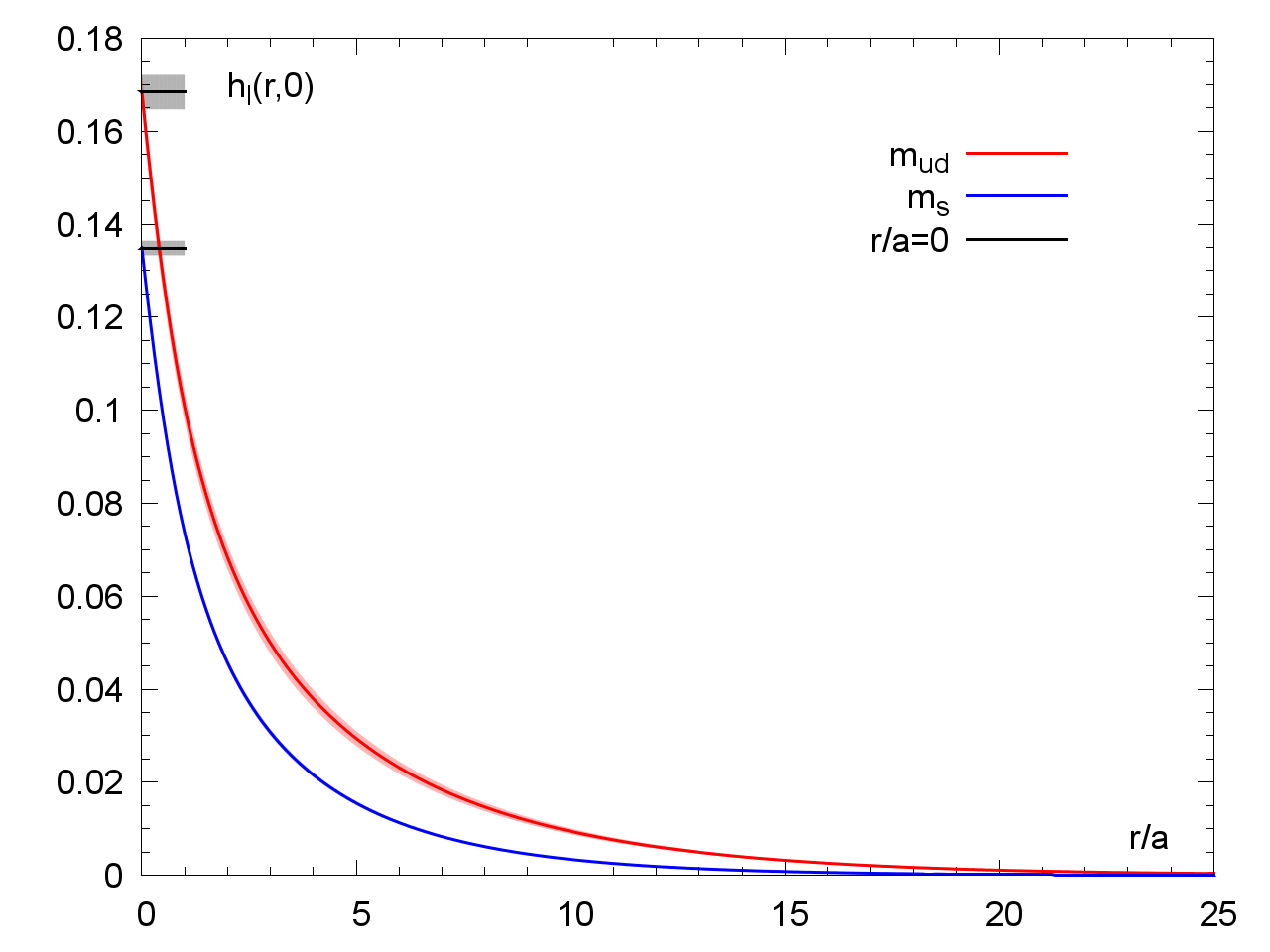
Figure 8: The hadronic vacuum polarization contribution $h_{l}(r,0)$ to the potential between two electric charges. Note that $r/a=20$ corresponds roughly to $r=1$fm.

IV Conclusion

We have studied two static properties of quantum relativistic plasmas. They represent a loop correction to the free energy of external static charges and stationary currents, where charge renormalization has been performed. In a hydrodynamic treatment, $\kappa_{t}$ enters the constitutive equation of the current and thus governs the linear response to an external magnetic field with a non-vanishing curl. We have calculated these two coefficients at one-loop order in perturbation theory for QED and using lattice QCD for the non-Abelian case. Remarkably, the presence of the plasma generates an antiscreening of electric currents and thereby an enhancement of the Ampère force between two currents. Our emphasis has been on the interpretation of these quantities and on the best suited strategies to compute them; in order to make a realistic prediction for QCD it would be necessary to explore the quark mass dependence and to take the continuum limit of the coefficients $\kappa_{l,t}$. While it appears unlikely that these physical effects have any observable consequence in primordial nucleosynthesis, it would be interesting to investigate further whether the coefficient $\kappa_{t}$ has any observable consequences, be it in the QED or in the QCD plasma.

Appendix A Treelevel calculation of $\kappa_{\ell}$ and $\kappa_{t}$

With $\tilde{j}_{1}(x_{3})=\int dx_{0}dx_{1}dx_{2}j_{1}(x)$, the coefficient $\kappa_{t}$ can be computed as follows,

$$\kappa_{t}=-\frac{\partial}{\partial(q_{3}^{2})}\int_{-\infty}^{\infty}dx_{3}\langle\tilde{j}_{1}(x_{3})j_{1}(0)\rangle|^{T}_{0}\;e^{iq_{3}x_{3}}\Big{|}_{q_{3}=0}=+\frac{1}{2}\int_{-\infty}^{\infty}dx_{3}\;x_{3}^{2}\langle\tilde{j}_{1}(x)j_{1}(0)\rangle|^{T}_{0}\;.$$ (68)

Using the spectral representation of the screening correlator,

$$-\langle\tilde{j}_{1}(x_{3})j_{1}(0)\rangle=\int_{0}^{\infty}\frac{d\omega}{2\pi}\;\tilde{\rho}_{11}(\omega,T)\;e^{-\omega|x_{3}|},$$ (69)

we obtain the expression

$$\kappa_{t}=-\frac{1}{\pi}\int_{0}^{\infty}\frac{d\omega}{\omega^{3}}\;(\tilde{\rho}_{11}(\omega,T)-\omega^{2}\rho^{\rm vac}(\omega^{2})).$$ (70)

Introducing the notation

$$p_{n}^{\pm}=(2n\pm 1)\pi T,\qquad E_{n}^{\pm}=(p_{n}^{\pm}{}^{2}+m^{2})^{1/2},$$ (71)

the spectral functions are given by, for $\omega\geq 0$,

$$\rho^{\rm vac}(\omega^{2}) = \frac{1}{6\pi}\sqrt{1-4m^{2}/\omega^{2}}\;(1+2m^{2}/\omega^{2})\;\theta(\omega-2m),$$ (72)

$$\tilde{\rho}_{11}(\omega,T) = \frac{\omega}{2\beta}\sum_{n=1}^{\infty}\left(1+\left({2E_{n}^{-}}/{\omega}\right)^{2}\right)\;\theta\left(\omega-2E_{n}^{-}\right).$$ (73)

We consider different intervals of frequency separately. From the low-frequency region, we get a purely vacuum contribution,

$$\kappa^{\rm low}=\frac{1}{\pi}\int_{0}^{2E_{0}^{+}}\frac{d\omega}{\omega}\rho^{\rm vac}(\omega^{2})=\frac{1}{36\pi^{2}}\left(6\,{\rm asinh\,}(\pi/(\beta m))-\frac{\pi(6\beta^{2}m^{2}+5\pi^{2})}{(\beta^{2}m^{2}+\pi^{2})^{3/2}}\right)$$ (74)

If we define $\tilde{\rho}_{11}(\omega,n,T)$ for $n\geq 1$ such that

$$\tilde{\rho}_{11}(\omega,n,T)=\tilde{\rho}_{11}(\omega,T)\qquad{\rm for}\qquad 2E_{n}^{-}\leq\omega\leq 2E_{n}^{+},$$ (75)

one finds

$$\tilde{\rho}_{11}(\omega,n,T)=\frac{n}{6\beta^{3}\omega}\left(3\beta^{2}(\omega^{2}+4m^{2})+4\pi^{2}(4n^{2}-1)\right).$$ (76)

Thus the coefficient $\kappa_{t}$ is given by

$$\kappa_{t} = \kappa^{\rm low}+\sum_{n=1}^{\infty}g_{b}(\beta,n),$$ (77)

$$g_{b}(\beta,n) \equiv -\frac{1}{\pi}\int_{2E_{n}^{-}}^{2E_{n}^{+}}\frac{d\omega}{\omega^{3}}\;(\tilde{\rho}_{11}(\omega,n,T)-\omega^{2}\rho^{\rm vac}(\omega^{2}))$$ (78)

The summand $g_{b}(\beta,n)$ is easily obtained analytically but the expression is not very illuminating and we do not reproduce it here. The series is absolutely convergent. Moreover, $g_{b}(\beta,n)$ can be expanded in positive powers of $\beta$, and each term in the expansion is an absolutely convergent series in $n$. The small $\beta m$ expansion is thus straightforwardly obtained in this way. Note that the infrared divergence in $\kappa_{t}$ when $m\to 0$ comes entirely from $\kappa^{\rm low}$.

For $\kappa_{\ell}$, the calculation proceeds in the same way,

$$\kappa_{\ell}=-\frac{1}{\pi}\int_{0}^{\infty}\frac{d\omega}{\omega^{3}}(\tilde{\rho}_{00}(\omega,T)-\omega^{2}\rho^{\rm vac}(\omega^{2})),$$ (79)

with the relevant screening spectral function given by

$$\tilde{\rho}_{00}(\omega,T)=\frac{\omega}{\beta}\sum_{n=1}^{\infty}\;(1-(2p_{n}^{-}/\omega)^{2})\;\theta\left(\omega-2E_{n}^{-}\right).$$ (80)

We then have

$$\tilde{\rho}_{00}(\omega,T)=\tilde{\rho}_{00}(\omega,n,T)\equiv\frac{n\,\omega}{\beta}+\frac{4\pi^{2}n(1-4n^{2})}{3\beta^{3}\omega},\qquad\quad 2E_{n}^{-}<\omega<2E_{n}^{+}.$$ (81)

Defining $g_{\ell}(\beta,n)$ analogously to $g_{b}(\beta,n)$ with $\tilde{\rho}_{11}$ replaced by $\tilde{\rho}_{00}$, we have $\kappa_{\ell}=\kappa^{\rm low}+\sum_{n=1}^{\infty}g_{\ell}(\beta,n)$.

The expansion (36) for $\kappa_{\ell}-\kappa_{t}=\sum_{n=1}^{\infty}[g_{\ell}(\beta,n)-g_{b}(\beta,n)]$, is obtained from

$$g_{\ell}(\beta,n)-g_{b}(\beta,n)=\frac{(p_{n}^{+}+p_{n}^{-})\,(E_{n}^{+}-E_{n}^{-})}{48\pi^{2}(E_{n}^{-}E_{n}^{+})^{3}}\left[(m^{2}+p_{n}^{+}p_{n}^{-})\,({E_{n}^{+}}^{2}+E_{n}^{+}E_{n}^{-}+{E_{n}^{-}}^{2})\,-3{E_{n}^{-}}^{2}{E_{n}^{+}}^{2}\right].$$ (82)

This expression can be expanded in positive powers of $\beta$, and then the individual Taylor coefficients can be summed over $n$. The series in $n$ are all absolutely convergent.

In order to obtain a representation more suitable for large values of $\beta m$, one uses the Poisson summation formula to rewrite the screening correlators

$$-\langle\tilde{j}_{\mu}(x_{3})j_{\mu}(0)\rangle=2\sum_{j\in\mathbb{Z}}(-1)^{j}\int\frac{d^{3}\boldsymbol{p}}{(2\pi)^{3}}\;\frac{e^{-2E_{\boldsymbol{p}}|x_{3}|+ip_{3}\beta j}}{E_{\boldsymbol{p}}^{2}}(E_{\boldsymbol{p}}^{2}-p_{\mu}^{2}),\qquad\textrm{(no summation over $\mu$; $\mu\neq 3$)}.$$ (83)

In particular one obtains $\kappa_{\ell}-\kappa_{t}$ by integrating the difference of the two correlators over $x_{3}$,

$$\kappa_{\ell}-\kappa_{t} = \int_{0}^{\infty}dx_{3}\,x_{3}^{2}\;\left\langle\tilde{j}_{0}(x_{3})j_{0}(0)-\tilde{j}_{1}(x_{3})j_{1}(0)\right\rangle$$ (84)

$$= -\frac{1}{8\pi^{2}}\sum_{j\in\mathbb{Z}\backslash\{0\}}(-1)^{j}\int_{0}^{\infty}\frac{p\,dp}{E_{p}^{5}}\;\left(p^{2}+3\frac{\partial^{2}}{j^{2}\partial\beta^{2}}\right)\frac{\sin(p\beta j)}{\beta j}.$$ (85)

Note that the term $j=0$ does not contribute, because it corresponds to the $T=0$ situation, where by rotation invariance the two correlators are equal. The integrals are now linear combinations of modified Bessel functions and we arrive at Eq. (36).

Appendix B Lattice perturbation theory

We consider a fermion described by the Wilson action. Defining

$$\hat{p}_{\mu}=\frac{2}{a}\sin\frac{ap_{\mu}}{2},\qquad\quad p^{{}^{\!\!\!\circ}}_{\mu}=\frac{1}{a}\sin ap_{\mu},\qquad\quad M_{p}=\frac{1}{2}a\hat{p}^{2}+m,$$ (86)

$$\int_{p}f(p)\equiv\frac{1}{\beta}\sum_{n_{0}=1}^{\beta/a}\int_{-\frac{\pi}{a}}^{\frac{\pi}{a}}\frac{d^{3}\boldsymbol{p}}{(2\pi)^{3}}~{}f({(2n_{0}-1)\pi}/{\beta},\boldsymbol{p}),$$ (87)

the propagator reads

$$G_{\rm w}(x,y)\equiv\langle\psi(x)\bar{\psi}(y)\rangle=\int_{p}\frac{e^{ip(x-y)}}{i\gamma_{\mu}p^{{}^{\!\!\!\circ}}_{\mu}+M_{p}}.$$ (88)

Consider the local vector current $\bar{\psi}(x)\gamma_{\mu}\psi(x)$ and the conserved vector current

$$V_{\mu}(x)=\frac{1}{2}\left(\bar{\psi}(x+a\hat{\mu})(1+\gamma_{\mu})U_{\mu}^{\dagger}(x)\psi(x)-\bar{\psi}(x)(1-\gamma_{\mu})U_{\mu}(x)\psi(x+a\hat{\mu})\right).$$ (89)

Its correlation function with the local current is

$$G^{\rm CL}_{\mu\nu}(x) \equiv -\langle V_{\mu}(x)\;\bar{\psi}(0)\gamma_{\nu}\psi(0)\rangle$$

$$= \frac{1}{2}{\rm Tr\,}\{(1+\gamma_{\mu})G(x,0)\gamma_{\nu}G(0,x+a\hat{\mu})-(1-\gamma_{\mu})G(x+a\hat{\mu})\gamma_{\nu}G(0,x)\}.$$

Inserting expression (88) for the fermion propagator and performing the Dirac traces, we obtain

$$a^{4}\sum_{x}G^{\rm CL}_{\mu\nu}(x)\,e^{ik(x+a\hat{\mu}/2)}\equiv-\Pi^{\rm CL}_{\mu\nu}(k)$$ (91)

$$={4}\int_{p}\frac{\cos[a(p_{\mu}+\frac{k_{\mu}}{2})](\delta_{\mu\nu}(p^{{}^{\!\!\!\circ}}\cdot q^{{}^{\!\!\!\circ}}+M_{p}M_{q})-p^{{}^{\!\!\!\circ}}_{\mu}q^{{}^{\!\!\!\circ}}_{\nu}-p^{{}^{\!\!\!\circ}}_{\nu}q^{{}^{\!\!\!\circ}}_{\mu})-\sin[a(p_{\mu}+\frac{k_{\mu}}{2})](M_{p}q^{{}^{\!\!\!\circ}}_{\nu}+M_{q}p^{{}^{\!\!\!\circ}}_{\nu})}{({p^{{}^{\!\!\!\circ}}}^{2}+M_{p}^{2})\;({q^{{}^{\!\!\!\circ}}}^{2}+M_{q}^{2})}\Big{|}_{q=p+k}.$$

The correlator satisfies

$$\sum_{\mu}\hat{k}_{\mu}\Pi^{\rm CL}_{\mu\nu}(k)=0.$$ (92)

Another representation is, on a spatial torus with infinite time extent,

$$a^{3}\sum_{\boldsymbol{x}}G_{11}^{\rm CL}(x) \stackrel{{\scriptstyle x_{0}\neq 0}}{{=}} \frac{4}{L_{1}L_{2}L_{3}}\sum_{\boldsymbol{p}}\frac{e^{-2\omega_{\boldsymbol{p}}|x_{0}|}}{D(\boldsymbol{p})^{2}}\Big{[}\cos(ap_{1})\left(D(\boldsymbol{p})^{2}/(2A(\boldsymbol{p}))^{2}+\boldsymbol{p^{{}^{\!\!\!\circ}}}^{2}-2p^{{}^{\!\!\!\circ}}{}^{2}_{1}+C(\boldsymbol{p})^{2}\right)-2ap^{{}^{\!\!\!\circ}}{}^{2}_{1}\,C(\boldsymbol{p})\Big{]},\qquad$$ (93)

$$a^{3}\sum_{\boldsymbol{x}}G_{11}^{\rm CL}(0,\boldsymbol{x}) = \frac{4}{L_{1}L_{2}L_{3}}\sum_{\boldsymbol{p}}\frac{1}{D(\boldsymbol{p})^{2}}\Big{[}\cos(ap_{1})\left(\boldsymbol{p^{{}^{\!\!\!\circ}}}^{2}-2p^{{}^{\!\!\!\circ}}{}^{2}_{1}+E(\boldsymbol{p})^{2}\right)-2ap^{{}^{\!\!\!\circ}}{}^{2}_{1}\,E(\boldsymbol{p})\Big{]}$$ (94)

with

$$A(\boldsymbol{p}) = 1+am+\frac{1}{2}a^{2}\hat{\boldsymbol{p}}^{2},\qquad B(\boldsymbol{p})=m^{2}+(1+am)\hat{\boldsymbol{p}}^{2}+\frac{1}{2}a^{2}\sum_{k<l}\hat{p}_{k}^{2}\hat{p}_{l}^{2}.$$ (95)

$$C(\boldsymbol{p}) = \frac{1}{2}a\hat{\boldsymbol{p}}^{2}+m-\frac{aB(\boldsymbol{p})}{2A(\boldsymbol{p})},\qquad D(\boldsymbol{p})=\sqrt{B(\boldsymbol{p})\,(4A(\boldsymbol{p})+a^{2}B(\boldsymbol{p}))},$$ (96)

$$E(\boldsymbol{p}) = C(\boldsymbol{p})+D(\boldsymbol{p})/(2A(\boldsymbol{p})),\qquad\omega_{\boldsymbol{p}}=\frac{2}{a}{\rm\,asinh\,}\left(\frac{a}{2}\sqrt{B(\boldsymbol{p})/A(\boldsymbol{p})}\right).$$ (97)

This representation is useful to calculate the $T=0$ vector correlator (in which case the $L_{i}$ can be sent to infinity) and the screening correlator at finite $T$ (in which case the direction $\boldsymbol{e}_{0}$ is interpreted as a spatial direction, while one of the directions $\boldsymbol{e}_{k}$ is interpreted as the Matsubara cycle). For the correlator of two local vector currents, see Aarts and Martinez Resco (2005).

References

- Arnold et al. (2012) P. Arnold, W. Florkowski, Z. Fodor, P. Foka, J. Harris, et al., PoS ConfinementX, 030 (2012).
- Thoma (2009) M. H. Thoma, J.Phys. A42, 214004 (2009), eprint 0809.1507.
- Gale (2012) C. Gale (2012), eprint 1208.2289.
- Shen et al. (2013) C. Shen, U. W. Heinz, J.-F. Paquet, and C. Gale (2013), eprint 1308.2440.
- Brandt et al. (2013) B. B. Brandt, A. Francis, H. B. Meyer, and H. Wittig, JHEP 1303, 100 (2013), eprint 1212.4200.
- Ding et al. (2011) H.-T. Ding, A. Francis, O. Kaczmarek, F. Karsch, E. Laermann, et al., Phys.Rev. D83, 034504 (2011), eprint 1012.4963.
- Amato et al. (2013) A. Amato, G. Aarts, C. Allton, P. Giudice, S. Hands, et al. (2013), eprint 1307.6763.
- Ghiglieri et al. (2013) J. Ghiglieri, J. Hong, A. Kurkela, E. Lu, G. D. Moore, et al., JHEP 1305, 010 (2013), eprint 1302.5970.
- Purcell (1963) E. M. Purcell, Electricity and Magnetism (Cambridge University Press, 1963).
- Hong and Teaney (2010) J. Hong and D. Teaney, Phys. Rev. C82, 044908 (2010), eprint 1003.0699.
- Baier et al. (2008) R. Baier, P. Romatschke, D. T. Son, A. O. Starinets, and M. A. Stephanov, JHEP 04, 100 (2008), eprint 0712.2451.
- Romatschke and Son (2009) P. Romatschke and D. T. Son, Phys. Rev. D80, 065021 (2009), eprint 0903.3946.
- Philipsen and Schaefer (2013) O. Philipsen and C. Schaefer, Lattice13 (2013).
- Weinberg (1995) S. Weinberg, The Quantum theory of fields. Vol. 1: Foundations (Cambridge University Press, 1995).
- Kapusta and Gale (2006) J. I. Kapusta and C. Gale, Finite-temperature field theory: Principles and applications (Cambridge University Press, 2006), 428.
- Olive (2012) K. A. Olive, AIP Conf.Proc. 1548, 116 (2012).
- Wilson (1974) K. G. Wilson, Phys. Rev. D10, 2445 (1974).
- Jansen and Sommer (1998) K. Jansen and R. Sommer (ALPHA collaboration), Nucl.Phys. B530, 185 (1998), eprint hep-lat/9803017.
- Hasenbusch (2001) M. Hasenbusch, Phys.Lett. B519, 177 (2001), eprint hep-lat/0107019.
- Hasenbusch and Jansen (2003) M. Hasenbusch and K. Jansen, Nucl.Phys. B659, 299 (2003), eprint hep-lat/0211042.
- Marinkovic and Schaefer (2010) M. Marinkovic and S. Schaefer, PoS LATTICE2010, 031 (2010), eprint 1011.0911.
- CLS (2010a) http://luscher.web.cern.ch/luscher/DD-HMC/index.html (2010a).
- Fritzsch et al. (2012) P. Fritzsch, F. Knechtli, B. Leder, M. Marinkovic, S. Schaefer, et al., Nucl.Phys. B865, 397 (2012), eprint 1205.5380.
- CLS (2010b) https://twiki.cern.ch/twiki/bin/view/CLS/WebIntro (2010b).
- Brandt et al. (2012) B. B. Brandt, A. Francis, H. B. Meyer, O. Philipsen, and H. Wittig (2012), eprint 1210.6972.
- Capitani et al. (2011) S. Capitani, M. Della Morte, G. von Hippel, B. Knippschild, and H. Wittig, PoS LATTICE2011, 145 (2011), eprint 1110.6365.
- Bochicchio et al. (1985) M. Bochicchio, L. Maiani, G. Martinelli, G. C. Rossi, and M. Testa, Nucl. Phys. B262, 331 (1985).
- Luscher et al. (1997) M. Lüscher, S. Sint, R. Sommer, P. Weisz, and U. Wolff, Nucl.Phys. B491, 323 (1997), eprint hep-lat/9609035.
- Guagnelli et al. (2001) M. Guagnelli et al. (ALPHA Collaboration), Nucl.Phys. B595, 44 (2001), eprint hep-lat/0009021.
- Della Morte et al. (2005a) M. Della Morte, R. Hoffmann, and R. Sommer, JHEP 0503, 029 (2005a), eprint hep-lat/0503003.
- Della Morte et al. (2009) M. Della Morte, R. Sommer, and S. Takeda, Phys.Lett. B672, 407 (2009), eprint 0807.1120.
- Della Morte et al. (2005b) M. Della Morte et al. (ALPHA Collaboration), Nucl.Phys. B729, 117 (2005b), eprint hep-lat/0507035.
- Della Morte et al. (2005c) M. Della Morte, R. Hoffmann, F. Knechtli, R. Sommer, and U. Wolff, JHEP 0507, 007 (2005c), eprint hep-lat/0505026.
- Luescher et al. (1996) M. Lüscher, S. Sint, R. Sommer, and P. Weisz, Nucl. Phys. B478, 365 (1996), eprint hep-lat/9605038.
- Sint and Weisz (1997) S. Sint and P. Weisz, Nucl.Phys. B502, 251 (1997), eprint hep-lat/9704001.
- Francis et al. (2013) A. Francis, B. Jäger, H. B. Meyer, and H. Wittig, Phys.Rev. D88, 054502 (2013), eprint 1306.2532.
- Laine and Vepsalainen (2004) M. Laine and M. Vepsalainen, JHEP 02, 004 (2004), eprint hep-ph/0311268.
- Aarts and Martinez Resco (2005) G. Aarts and J. M. Martinez Resco, Nucl. Phys. B726, 93 (2005), eprint hep-lat/0507004.