On the Observability of the Quark Orbital Angular Momentum Distribution

Abstract

We argue that due to Parity constraints, the helicity combination of the purely momentum space counterparts of the Wigner distributions – the generalized transverse momentum distributions – that describes the configuration of an unpolarized quark in a longitudinally polarized nucleon, can enter the deeply virtual Compton scattering amplitude only through matrix elements involving a final state interaction. The relevant matrix elements in turn involve light cone operators projections in the transverse direction, or they appear in the deeply virtual Compton scattering amplitude at twist three. Orbital angular momentum or the spin structure of the nucleon was a major reason for these various distributions and amplitudes to have been introduced. We show that the twist three contributions associated to orbital angular momentum are related to the target-spin asymmetry in deeply virtual Compton scattering, already measured at HERMES.

1. Considerable attention has been devoted to the partons’ Transverse Momentum Distributions (TMDs), to the Generalized Parton Distributions (GPDs), and to finding a connection between the two Bur ; Metz1 ; Metz2 . TMDs are distributions of different spin configurations of quarks and gluons within the nucleon whose longitudinal and transverse momenta can be accessed in Semi-Inclusive Deep Inelastic Scattering (SIDIS). GPDs are real amplitudes for quarks or gluons being probed in a hard process and then returning to reconstitute a scattered nucleon. They are accessed through exclusive electroproduction of vector bosons along with the nucleon. In each case there is a nucleon matrix element of bilinear, non-local quark or gluon field operators. In principle both TMDs and GPDs are different limits of Wigner distributions, i.e. the phase space distributions in momenta and impact parameters. The purely momentum space form of those are the Generalized TMDs (GTMDs). GTMDs correlate hadronic states with same parton longitudinal momentum, $x$ (assuming zero skewness), different relative transverse distance, ${\bf z}_{T}={\bf b}_{in}-{\bf b}_{out}$, between the struck parton’s initial and final (out) states, and same average transverse distance, ${\bf b}=({\bf b}_{in}+{\bf b}_{out})/2$, of the struck parton with respect to the center of momentum Soper77 (Figure 1a).

Understanding the angular momentum or spin structure of the nucleon is a major reason for these various distributions and amplitudes to have been introduced.

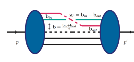
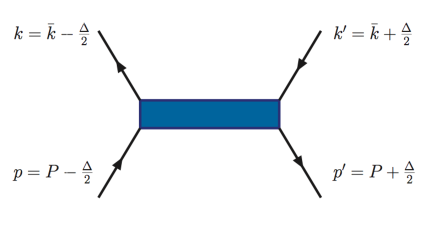
Figure 1: (a) Left: Correlation function for a GTMD; (b) quark-proton scattering in the $u$-channel.

Recently, specific GTMDs and Wigner distributions were studied that are thought to be related to the more elusive component of the angular momentum sum rule, which is partonic Orbital Angular Momentum (OAM) Vento ; Brodsky ; LorPas ; Yuan . Such theoretical efforts have been developing in parallel with the realization that the leading twist contribution to the angular momentum sum rule comes from transverse spin Ji_Xiong , while longitudinal angular momentum, and consequently orbital angular momentum, can be associated with twist three partonic components. The GTMD that was proposed to describe OAM appears in the parametrization of the (leading order) vector, $\gamma^{+}$, component of the unintegrated quark-quark correlator for the proton given in Metz2 as,

$$\bar{u}(p^{\prime},\Lambda^{\prime})\frac{i\sigma^{ij}\bar{k}_{T}^{i}\Delta_{T}^{j}}{M^{2}}u(p,\Lambda)F_{14}\propto\langle{\bf S}_{L}\cdot\bar{\bf k}_{T}\times{\bf\Delta}_{T}\rangle.$$ (1)

where $(p,\Lambda),(p^{\prime},\Lambda^{\prime})$ are the proton’s initial and final momentum and helicity, $k_{T}$ and $\Delta_{T}$ are the quarks’ average and relative momenta, respectively, and $F_{14}$ is the GTMD defined according to the classification scheme of Metz2 . Eq.(1) appears to represent the distribution of an unpolarized quark in a longitudinally polarized proton ($\rho_{LU}$ in Ref.LorPas ). However, we notice that its observability is inconsistent with several physical properties, namely:

i) it drops out of the formulation of both GPDs and TMDs, so that it cannot be measured;

ii) it is Parity-odd. Notice, in fact, how this structure is at variance with the more familiar $\langle{\bf S}_{T}\times\bar{\bf k}_{T}\rangle$ term, defining the TMD Sivers function Sivers , which is a Parity even observable with an analogous asymmetry but for transverse spin. It also differs from the definition of OAM based on the TMD $h_{1T}^{\perp}$ Avakian ; Ma , in that the latter also exhibits a transverse spin structure.

iii) it is non zero only for imaginary values of the quark-proton helicity amplitudes.

In order to develop a more concrete understanding of OAM that could lead to the definition of specific observables, it is important to examine the newly proposed partonic configurations and their connection with the quark-proton helicity or transverse spin amplitudes. In this paper, after showing the constraints on the recently studied GTMDs from the invariance under Parity transformations, we perform a thorough analysis of their helicity/transverse spin structure. We suggest that the helicity structure giving rise to OAM is described by twist three distributions only. Our findings corroborate the interpretation of the spin sum rule including OAM originally given in Polyakov (see also Penttinen ; Hatta ). Using the formalism proposed in Ref. Metz2 ; BelMuel , we identify the integrals over transverse momentum of the twist three GTMDs with twist three GPDs. The latter enter the $\sin 2\phi$ modulation of the target-spin asymmetry, $A_{UL}$, in DVCS which has already been measured at both HERMES HERMES and JLab pisano_privcomm . We present here predictions for $A_{UL}^{\sin 2\phi}$ using the GPD set of Ref. GGL ; GGL_FF . This is the first proposal for a direct experimental access to orbital angular momentum.

2. In Ref. Metz2 it was found that with Parity invariance, time reversal invariance, and Hermiticity there are 16 independent complex GTMDs for the quark-nucleon system, corresponding to 16 helicity amplitudes for quark-nucleon elastic scattering. However, we know that for elastic 2-body scattering of two spin $1/2$ particles there will only be 8 independent amplitudes. This follows from implementing Parity transformations on the helicity amplitudes in the 2-body Center of Mass (CM) frame JacobWick where all the incoming and outgoing particles are confined to a plane. In this plane the Parity transformation flips all momenta but it does not change the relation among the momentum components. In any other frame there will still be 8 independent amplitudes, although they may be in linear combinations with kinematic factors that appear to yield 16. The counting of helicity amplitudes in polarization dependent high energy scattering processes was addressed e.g. Ref. FGM . In order to explain this point, and to investigate its consequences on the off-forward matrix elements of QCD correlators, we first start by reviewing the helicity structure of the GTMDs from Ref.Metz2 .

To describe quark-proton scattering as a $u$-channel two-body scattering process (Fig.1b)

$$q^{\prime}(k^{\prime})+N(p)\rightarrow q(k)+N^{\prime}(p^{\prime}),$$

we choose a Light-Cone (LC) frame, where the average and relative 4-momenta $P=(p+p^{\prime})/2$, $\bar{k}=(k+k^{\prime})/2$, $\Delta=p^{\prime}-p=k^{\prime}-k$, respectively have components specified by,

$$P \equiv \left(P^{+},\frac{{\bf\Delta}_{T}^{2}+4M^{2}}{8P^{+}},0\right)$$ (2a)

$$\bar{k} \equiv \left(xP^{+},k^{-},\bar{\bf k}_{T}\right)$$ (2b)

$$\Delta \equiv \left(0,0,{\bf\Delta}_{T}\right)$$ (2c)

where $v\equiv(v^{+},v^{-},{\bf v}_{T})$, $v^{\pm}=1/\sqrt{2}(v_{o}\pm v_{3})$, and for simplicity we have taken the skewness variable, $\xi=0$ since this will not enter our discussion.

The connection between the unintegrated matrix elements defining the GTMDs and the quark-proton helicity amplitudes is obtained by considering the quark-proton helicity amplitude (Fig.1 and Ref.Diehl_rev ),

$$A_{\Lambda^{\prime}\lambda^{\prime},\Lambda\lambda}=\int\frac{dz^{-}\,d^{2}{\bf z}_{T}}{(2\pi)^{3}}e^{ixP^{+}z^{-}-i\bar{\bf k}_{T}\cdot{\bf z}_{T}}\left.\langle p^{\prime},\Lambda^{\prime}\mid{\cal O}_{\lambda^{\prime}\lambda}(z)\mid p,\Lambda\rangle\right|_{z^{+}=0},$$

where in the chiral even sector,

$${\cal O}_{\pm\pm}(z) = \bar{\psi}\left(-\frac{z}{2}\right)\gamma^{+}(1\pm\gamma_{5})\psi\left(\frac{z}{2}\right).$$ (4)

Following the definitions in Ref. Metz2 , and making use of the Gordon decomposition,

$$\overline{U}(p^{\prime},\Lambda^{\prime})\gamma^{\mu}U(p,\Lambda)=\overline{U}(p^{\prime},\Lambda^{\prime})\frac{P^{\mu}}{M}U(p,\Lambda)+\overline{U}(p^{\prime},\Lambda^{\prime})\frac{i\sigma^{i\,\mu}\Delta_{i}}{2M}U(p,\Lambda),$$ (5)

we obtain for the vector case,

$$W^{\gamma^{+}}_{\Lambda\Lambda^{\prime}} = \frac{1}{2P^{+}}\left[\overline{U}(p^{\prime},\Lambda^{\prime})\gamma^{+}U(p,\Lambda)F_{11}+\overline{U}(p^{\prime},\Lambda^{\prime})\frac{i\sigma^{i+}\Delta_{T}^{i}}{2M}U(p,\Lambda)(2F_{13}-F_{11})\right.$$ (6)

$$+ \left.\overline{U}(p^{\prime},\Lambda^{\prime})\frac{i\sigma^{i+}\bar{k}_{T}^{i}}{2M}U(p,\Lambda)(2F_{12})+\overline{U}(p^{\prime},\Lambda^{\prime})\frac{i\sigma^{ij}\bar{k}_{T}^{i}\Delta_{T}^{j}}{M^{2}}U(p,\Lambda)\,F_{14}\right]$$

$$= \delta_{\Lambda,\Lambda^{\prime}}F_{11}+\delta_{\Lambda,-\Lambda^{\prime}}\frac{-\Lambda\Delta_{1}-i\Delta_{2}}{2M}(2F_{13}-F_{11})+\delta_{\Lambda,-\Lambda^{\prime}}\frac{-\Lambda\bar{k}_{1}-i\bar{k}_{2}}{2M}(2F_{12})+\delta_{\Lambda,\Lambda^{\prime}}i\Lambda\frac{\bar{k}_{1}\Delta_{2}-\bar{k}_{2}\Delta_{1}}{M^{2}}F_{14},$$

and for the axial-vector case,

$$W^{\gamma^{+}\gamma_{5}}_{\Lambda\Lambda^{\prime}} = \frac{1}{2\,{P}^{+}}\left[-\overline{U}(p^{\prime},\Lambda^{\prime})\frac{i\epsilon_{T}^{ij}\,\bar{k}_{T}^{i}\Delta_{T}^{j}}{M^{2}}\,\frac{2P^{+}}{2M}U(p,\Lambda)G_{11}+\overline{U}(p^{\prime},\Lambda^{\prime})\frac{i\sigma^{i+}\gamma_{5}\Delta_{T}^{i}}{2M}U(p,\Lambda)(2G_{13})\right.$$

$$+ \left.\overline{U}(p^{\prime},\Lambda^{\prime})\frac{i\sigma^{i+}\gamma_{5}\,\bar{k}_{T}^{i}}{2M}U(p,\Lambda)(2G_{12})+\overline{U}(p^{\prime},\Lambda^{\prime})i\sigma^{+-}\gamma_{5}U(p,\Lambda)\,G_{14}\right]$$

$$= \delta_{\Lambda,\Lambda^{\prime}}\Lambda G_{14}+\delta_{\Lambda,-\Lambda^{\prime}}\frac{\Delta_{1}+i\Lambda\Delta_{2}}{2M}\,2G_{13}+\delta_{\Lambda,-\Lambda^{\prime}}\frac{\bar{k}_{1}+i\Lambda\bar{k}_{2}}{2M}\,2G_{12}-\delta_{\Lambda,\Lambda^{\prime}}i\frac{\bar{k}_{1}\Delta_{2}-\bar{k}_{2}\Delta_{1}}{M^{2}}G_{11},$$

By summing and subtracting the two equations, one obtains the following expressions for the quark-proton helicity amplitudes,

$$A_{\Lambda^{\prime}+,\Lambda,+} = \delta_{\Lambda,\Lambda^{\prime}}(F_{11}+\Lambda G_{14}+i\Lambda\frac{\bar{k}_{1}\Delta_{2}-\bar{k}_{2}\Delta_{1}}{M^{2}}F_{14}-i\frac{\bar{k}_{1}\Delta_{2}-\bar{k}_{2}\Delta_{1}}{M^{2}}G_{11})+$$

$$\delta_{\Lambda,-\Lambda^{\prime}}\left[\frac{-\Lambda\Delta_{1}-i\Delta_{2}}{2M}(2F_{13}-F_{11})+\frac{\Delta_{1}-i\Lambda\Delta_{2}}{2M}2G_{13}+\frac{-\Lambda\bar{k}_{1}-i\bar{k}_{2}}{2M}2F_{12}+\frac{\bar{k}_{1}-i\Lambda\bar{k}_{2}}{2M}2G_{12}\right]$$

$$A_{\Lambda^{\prime}-,\Lambda,-} = \delta_{\Lambda,\Lambda^{\prime}}(F_{11}-\Lambda G_{14}+i\Lambda\frac{\bar{k}_{1}\Delta_{2}-\bar{k}_{2}\Delta_{1}}{M^{2}}F_{14}+i\,\frac{\bar{k}_{1}\Delta_{2}-\bar{k}_{2}\Delta_{1}}{M^{2}}G_{11})+$$

$$\delta_{\Lambda^{\prime},-\Lambda}\left[\frac{-\Lambda\Delta_{1}-i\Delta_{2}}{2M}(2F_{13}-F_{11})-\frac{\Delta_{1}-i\Lambda\Delta_{2}}{2M}2G_{13}+\frac{-\Lambda\bar{k}_{1}-i\bar{k}_{2}}{2M}2F_{12}-\frac{\bar{k}_{1}-i\Lambda\bar{k}_{2}}{2M}2G_{12}\right],$$

We now examine the new contributions, $F_{14}$, and $G_{11}$,

$$i\frac{\bar{k}_{1}\Delta_{2}-\bar{k}_{2}\Delta_{1}}{M^{2}}F_{14} = A_{++,++}+A_{+-,+-}-A_{-+,-+}-A_{--,--}$$ (9a)

$$-i\frac{\bar{k}_{1}\Delta_{2}-\bar{k}_{2}\Delta_{1}}{M^{2}}G_{11} = A_{++,++}-A_{+-,+-}+A_{-+,-+}-A_{--,--}$$ (9b)

$F_{14}$ describes an unpolarized quark in a longitudinally polarized proton, while $G_{11}$ describes a longitudinally polarized quark in an unpolarized proton.

We reiterate, however, that Parity, imposes limits on the possible polarization asymmetries that can be observed in two body scattering: because of 4-momentum conservation and on-shell conditions, $k^{2}=m^{2}$, $p^{2}=M^{2}$, there are eight variables. Four of those describe the energy and 3-momentum of the CM relative to a fixed coordinate system, while the remaining four give the energy and the 3-vector orientation and magnitude of the scattering plane in the CM. In the CM frame or, equivalently in the “lab” frame with the $p$ direction chosen as the $z$-direction, the net longitudinal polarization defined in Eq.(1), is clearly a Parity violating term (pseudoscalar) under space inversion. This implies that a measurement of single longitudinal polarization asymmetries would violate Parity conservation in an ordinary two body scattering process corresponding to tree level, twist two amplitudes. Releasing the partons’ on-shell condition implies introducing higher twists in the description of the process EFP We can therefore anticipate that similarly to the TMDs $g^{\perp},f_{L}^{\perp},\ldots$ in SIDIS, single longitudinal polarization asymmetries are higher twist objects.

On the other hand, notice that polarization along the normal to the scattering plane is Parity conserving (scalar) under spatial inversion, thus giving rise to SSAs at leading twist JacRobRos .

To be explicit regarding parity constraints consider again the helicity amplitudes for the 2-body process,

$$A_{\Lambda^{\prime},\,\lambda^{\prime};\,\Lambda,\,\lambda}:q^{\prime}(k^{\prime},\lambda^{\prime})+N(p,\Lambda)\rightarrow q(k,\lambda)+N^{\prime}(p^{\prime},\Lambda^{\prime}).$$ (10)

Such amplitudes can be written in any Lorentz frame, but in the Center of Momentum frame the parity relations are simple,

$$A_{-\Lambda^{\prime},\,-\lambda^{\prime};\,-\Lambda,\,-\lambda}=(-1)^{\eta}\,A_{\Lambda^{\prime},\,\lambda^{\prime};\,\Lambda,\,\lambda}^{*},$$ (11)

where $\eta=\Lambda^{\prime}-\lambda^{\prime}-\Lambda+\lambda$, the net helicity change. Hence of 16 possible helicity amplitudes, 8 are independent. For chiral even, non-flip nucleon amplitudes there are 2 independent. These determinations are made in the CoM frame. By Lorentz covariance and 4-momentum conservation, the number of independent amplitudes cannot change. In other frames, e.g. the light cone frame or the target rest frame, there may appear to be more, yet the extra amplitudes must be linear combinations of the independent ones. In particular

$$A_{\widetilde{\Lambda}^{\prime},\,\widetilde{\lambda}^{\prime};\,\widetilde{\Lambda},\,\widetilde{\lambda}}=\sum_{\Lambda^{\prime},\cdots}D_{\widetilde{\Lambda}^{\prime},\,\Lambda^{\prime}}^{1/2}(\Omega_{N}^{\prime})\cdots A_{\Lambda^{\prime},\,\lambda^{\prime};\,\Lambda,\,\lambda},$$ (12)

where the $D$ functions are the rotation matrices for the Wigner rotations, $\Omega_{N}^{\prime}$, etc.

We see that for $F_{14}$ in Eq. 9a and $G_{11}$ in Eq. 9b to be non-zero there must be an imaginary part to either $A_{++;++}$ or $A_{+-;+-}$. This will not be the case in the CoM frame, wherein the momenta are coplanar. In order to have a non-vanishing helicity amplitude combination there must be another independent direction. That is provided by twist three amplitudes and corresponding GTMDs, as we show below.

Note also that that in the parametrization of the generalized correlation function of Ref.Metz2 ,

$$W_{\Lambda^{\prime},\,\Lambda}^{\gamma^{+}} = {\overline{U}}(p^{\prime},\Lambda^{\prime})\left[\overbrace{\frac{P^{+}}{M}(A_{1}^{F}+xA_{2}^{F}-2\xi A_{3}^{F})}^{type1}+\overbrace{\frac{i\sigma^{+k}}{M}A_{5}^{F}+\frac{i\sigma^{+\Delta}}{M}A_{6}^{F}}^{type2}+\overbrace{\frac{P^{+}i\sigma^{k\,\Delta}}{M^{3}}(A_{8}^{F}+xA_{9}^{F})}^{type3}\right.$$ (13)

$$\left.+\underbrace{\frac{P^{+}i\sigma^{k\,N}}{M^{3}}(A_{11}^{F}+xA_{12}^{F})+\frac{P^{+}i\sigma^{\Delta\,N}}{M^{3}}(A_{14}^{F}-2\xi A_{15}^{F})}_{type4}\right]U(p,\Lambda)$$

$$= A_{\Lambda^{\prime}\,+;\Lambda\,+}^{[\gamma^{+}]}+A_{\Lambda^{\prime}\,-;\Lambda\,-}^{[\gamma^{+}]}$$

the Dirac structure reduces to the four distinct groups selected above, of which type 1,2 and 4 are Parity even, while type 3, which composes $F_{14}$, is Parity odd SL_talkQCDJlab (details of the calculation will be given in inprogress ). Because of the Parity constraints Metz2 $F_{14}$ can therefore be non zero only if its corresponding helicity amplitudes combination is imaginary. Hence it cannot have a straightforward partonic interpretation. Integrating over $k_{T}$ gives zero for $F_{14}$ meaning that this term decouples from partonic angular momentum sum rules. The vector GPDs can, in fact, be written in terms of GTMDs as Metz2 ,

$$H = \int d^{2}\bar{\bf k}_{T}F_{11}$$ (14)

$$E = \int d^{2}\bar{\bf k}_{T}\left[-F_{11}+2\left(\frac{\bar{\bf k}_{T}\cdot{\bf\Delta}}{\Delta^{2}}F_{12}+F_{13}\right)\right].$$ (15)

We conclude that type 3 should not be included in the leading twist parametrization in Eq.(6). A similar argument is valid for the axial vector component (Eq.(On the Observability of the Quark Orbital Angular Momentum Distribution)).

3. In the presence of final state interactions Parity relations apply differently. We will show that the combination

$$A_{++,++}+A_{+-,+-}-A_{-+,-+}-A_{--,--},$$

gets replaced by a similar helicity structure where now the longitudinal spin is crossed into ${\bf\Delta}$, namely $\langle{\bf S}_{L}\times{\bf\Delta}_{T}\rangle$. Notice that this produces a transverse angular momentum component rather than the longitudinal component appearing in Eq.(1).

The chiral-even twist three components were also parametrized in Ref.Metz2 ,

$$W^{\gamma^{i}}_{\Lambda^{\prime}\Lambda} = \frac{1}{2P^{+}}\overline{U}(p^{\prime},\Lambda^{\prime})\left[\frac{\bar{k}_{T}^{i}}{M}F_{21}+\frac{\Delta_{T}^{i}}{M}(F_{22}-2F_{26})+\frac{i\sigma^{ji}\bar{k}_{T}^{j}}{M}F_{27}+\gamma^{i}(2F_{28})\right.$$ (16)

$$+ \left.\frac{Mi\sigma^{i+}}{P^{+}}F_{23}+\frac{\bar{k}_{T}^{i}}{M}\frac{i\sigma^{k+}\bar{k}_{T}^{k}}{P^{+}}F_{24}+\frac{\Delta_{T}^{i}}{M}\frac{i\sigma^{k+}\bar{k}_{T}^{k}}{P^{+}}F_{25}+\frac{\Delta_{T}^{i}}{P^{+}}\gamma^{+}(2F_{26})\right]U(p,\Lambda),$$

where we used the Gordon identity (5) in order to connect the helicity structure of the twist three tensor to the approaches in BelMuel ; Polyakov . The first four terms in Eq. (16) conserve the proton helicity, while the last four terms flip the proton helicity. Furthermore we used the identity

$$\overline{U}(p^{\prime},\Lambda^{\prime})\gamma_{i}U(p,\Lambda)=\overline{U}(p^{\prime},\Lambda^{\prime})\frac{i\sigma^{ji}\,\Delta_{T}^{j}}{M}U(p,\Lambda)\rightarrow\left\langle{\bf S}_{L}\times{\bf\Delta}_{T}\right\rangle.$$

Using the notation of Eq. (4), we now consider the matrix elements of the quark twist three operators,

$${\cal O}^{q}_{\pm\mp}(z) = \bar{\psi}\left(-\frac{z}{2}\right)(\gamma_{1}\pm i\gamma_{2})(1\pm\gamma_{5})\psi\left(\frac{z}{2}\right),$$ (17)

which lead to the following expression for the helicity amplitude,

$$A^{tw3}_{\Lambda^{\prime}\lambda^{\prime},\Lambda\lambda} =\displaystyle\int\frac{dz^{-}\,d^{2}{\bf z}_{T}}{(2\pi)^{3}}e^{ixP^{+}z^{-}-i\bar{\bf k}_{T}\cdot{\bf z}_{T}}\left.\langle p^{\prime},\Lambda^{\prime}\mid{\cal O}_{\lambda^{\prime}-\lambda}(z)\mid p,\Lambda\rangle\right|_{z^{+}=0},$$ (18)

where now,

$${\cal O}^{q}_{\pm\mp}(z) = \phi^{\dagger}_{\pm}\left(-\frac{z}{2}\right)\chi_{\pm}\left(\frac{z}{2}\right)\pm\,\chi^{\dagger}_{\pm}\left(-\frac{z}{2}\right)\phi_{\pm}\left(\frac{z}{2}\right).$$ (19a)

For the good spinor components, $\phi_{\lambda}$, helicity and chirality are the same since ($1\pm\gamma^{5}$) projects out both $\pm$ helicity and chirality. For the bad components helicity and chirality are opposite as it follows from the fact that $\chi_{\lambda}$ describes a composite system of a transverse gluon and $\phi_{\lambda}$. Since the gluon carries helicity but no chirality, by imposing angular momentum conservation one obtains the opposite chirality KogSop ; Jaffe . The net effect of this distinction between helicity and chirality is that the helicity conserving quark correlator at twist three will behave like the chirality odd operator at twist two - the latter flips helicity. That is interpreted as if the genuine twist three correlator has the helicity of the returning quark flipped ($\pm 1/2\rightarrow\mp 1/2$), while the collinear gluon field is transverse and with compensating helicity ($\pm 1$) Jaffe . The implication for the Parity relations, unlike Eq.(11), is that the reversed helicities are not directly related to the initial set. The twist three correlator does not map directly onto a 2-body process. For this reason there are twice as many vector and axial vector twist three GPDs and TMDs.

As we have noted, for the non flip quark-proton helicity amplitudes at twist three one finds that the chiral even structures correspond to what would be chiral odd at twist two,

$$A^{tw3}_{\Lambda^{\prime}\pm,\Lambda\pm}\rightarrow A^{tw2}_{\Lambda^{\prime}\pm,\Lambda\mp}.$$ (20)

By using the operators in Eq. (19), the non-flip helicity amplitudes ($\Lambda=\Lambda^{\prime}$) can be read off from the hadronic tensors parameterizations as,

$$A^{tw3}_{\Lambda+,\Lambda+} = \frac{\bar{k}_{T}^{1}+i\bar{k}_{T}^{2}}{P^{+}}F_{21}+\frac{\Delta_{1}+i\Delta_{2}}{P^{+}}F_{22}-\Lambda\frac{\bar{k}_{T}^{1}+i\bar{k}_{T}^{2}}{P^{+}}F_{27}-\Lambda\frac{\Delta_{T}^{1}+i\Delta_{T}^{2}}{P^{+}}F_{28}$$ (21a)

$$+ \frac{\bar{k}_{T}^{1}+i\bar{k}_{T}^{2}}{P^{+}}G_{21}+\frac{\Delta_{1}+i\Delta_{2}}{P^{+}}G_{22}+\Lambda\frac{\bar{k}_{T}^{1}+i\bar{k}_{T}^{2}}{P^{+}}G_{27}+\Lambda\frac{\Delta_{T}^{1}+i\Delta_{T}^{2}}{P^{+}}G_{28}$$

$$A^{tw3}_{\Lambda-,\Lambda-} = \frac{\bar{k}_{T}^{1}-i\bar{k}_{T}^{2}}{P^{+}}F_{21}+\frac{\Delta_{1}-i\Delta_{2}}{P^{+}}F_{22}+\Lambda\frac{\bar{k}_{T}^{1}-i\bar{k}_{T}^{2}}{P^{+}}F_{27}+\Lambda\frac{\Delta_{T}^{1}-i\Delta_{T}^{2}}{P^{+}}F_{28}$$ (21b)

$$+ \frac{\bar{k}_{T}^{1}-i\bar{k}_{T}^{2}}{P^{+}}G_{21}+\frac{\Delta_{1}-i\Delta_{2}}{P^{+}}G_{22}+\Lambda\frac{\bar{k}_{T}^{1}-i\bar{k}_{T}^{2}}{P^{+}}G_{27}+\Lambda\frac{\Delta_{T}^{1}-i\Delta_{T}^{2}}{P^{+}}G_{28}$$

Only two independent combinations of the $A^{tw3}_{\Lambda\lambda,\Lambda\lambda}$ can be formed, namely,

$$\frac{4}{P^{+}}\left[\frac{\bar{\bf k}_{T}\cdot{\bf\Delta}_{T}}{\Delta_{T}}F_{21}+\Delta_{T}F_{22}+\left(\frac{\bar{\bf k}_{T}\cdot{\bf\Delta}_{T}}{\Delta_{T}}G_{21}+\Delta_{T}G_{22}\right)\right] = A_{++,++}^{tw3}+A_{+-,+-}^{tw3}+A_{-+,-+}^{tw3}+A_{--,--}^{tw3}$$ (22a)

$$-\frac{4}{P^{+}}\left[\frac{\bar{\bf k}_{T}\cdot{\bf\Delta}_{T}}{\Delta_{T}}F_{27}+\Delta_{T}F_{28}-\left(\frac{\bar{\bf k}_{T}\cdot{\bf\Delta}_{T}}{\Delta_{T}}G_{27}+\Delta_{T}G_{28}\right)\right] = A_{++,++}^{tw3}+A_{+-,+-}^{tw3}-A_{-+,-+}^{tw3}-A_{--,--}^{tw3}$$ (22b)

where we have taken ${\bf\Delta}_{T}$ along the $x$-axis without loss of generality. Notice that Eq.(22a) corresponds to the unpolarized case yielding the twist two GPD $H$, while Eq.(22b) gives the distribution of an unpolarized quark in a longitudinally polarized proton. Owing to the helicity structure of the twist three quark operators discussed above, this combination is now allowed by Parity conservation KogSop ; Jaffe .

Integrating over ${\bf\bar{k}_{T}}$, one obtains the twist three GPDs,

$$2\widetilde{H}_{2T}+E_{2T} = \int d^{2}{\bf k}_{T}\left[\left(\frac{{\bf k}_{T}\cdot{\bf\Delta}_{T}}{\Delta_{T}^{2}}\right)F_{21}+F_{22}\right]$$ (23)

$$\widetilde{E}_{2T} = -2\int d^{2}{\bf k}_{T}\left[\left(\frac{{\bf k}_{T}\cdot{\bf\Delta}_{T}}{\Delta_{T}^{2}}\right)F_{27}+F_{28}\right]$$ (24)

$$2\widetilde{H}_{2T}^{\prime}+E_{2T}^{\prime} = \int d^{2}{\bf k}_{T}\left[\left(\frac{{\bf k}_{T}\cdot{\bf\Delta}_{T}}{\Delta_{T}^{2}}\right)G_{21}+G_{22}\right]$$ (25)

$$\widetilde{E}_{2T}^{\prime} = -2\int d^{2}{\bf k}_{T}\left[\left(\frac{{\bf k}_{T}\cdot{\bf\Delta}_{T}}{\Delta_{T}^{2}}\right)G_{27}+G_{28}\right]$$ (26)

in agreement with Ref.Metz2 . In order to proceed, it is important to connect the various notations for the twist three GPDs which appear classified in the literature in the three main publications, Refs. BelMuel ; Polyakov ; Metz2 , respectively. By using the Gordon relation and Kivel

$$i\epsilon^{+i\alpha\beta}\overline{U}(p^{\prime},\Lambda^{\prime})\gamma_{\alpha}\Delta_{\beta}\gamma_{5}U(p,\Lambda)=i\overline{U}(p^{\prime},\Lambda^{\prime})\left(\Delta_{j}\gamma^{+}-\Delta_{+}\gamma^{j}\right)\gamma_{5}U(p,\Lambda)=2P^{+}\overline{U}(p^{\prime},\Lambda^{\prime})\gamma^{j}U(p,\Lambda),$$

which follows from the Dirac equation, we find that all notations, as reported in Table 1, are equivalent.

Polyakov et al. Polyakov	$2G_{1}$	$G_{2}$	$G_{3}$	$G_{4}$
Meissner et al. Metz2	$2\widetilde{H}_{2T}$	$\widetilde{E}_{2T}$	$E_{2T}$	$H_{2T}$
Belitsky et al. BelMuel	$E_{+}^{3}$	$\widetilde{H}_{-}^{3}$	$H_{+}^{3}+E_{+}^{3}$	$\displaystyle\frac{1}{\xi}\widetilde{E}_{-}^{3}$

Table 1: Comparison of notations for different twist 3 GPDs.

.

4. We now turn to the interpretation of the OAM term in the proton’s angular momentum sum rule JM_SR ; Ji_SR which requires, as we show below, the twist three helicity amplitudes combination corresponding to $\widetilde{E}_{2T}$, Eq.(24). While the derivation of the sum rule was carried out along similar lines in both Refs.JM_SR and Ji_SR , the two approaches essentially differ in that in Ref.JM_SR (JM) one has,

$$\frac{1}{2}=\frac{1}{2}\Delta\Sigma+{\cal L}_{q}+\Delta G+{\cal L}_{g},$$ (27)

where ${\cal L}_{q(g)}\rightarrow{\bf r}\times i{\bf\partial}$, i.e. corresponds to canonical OAM, while in Ref.Ji_SR (Ji),

$$\frac{1}{2}=J_{q}+J_{g}=\frac{1}{2}\Delta\Sigma+L_{q}+J_{g},$$ (28)

where $L_{q}\rightarrow{\bf r}\times i{\bf D}$ includes dynamics through the covariant derivative. $J_{g}$, the gluons total angular momentum contribution to Eq.(28) was originally not split into its separate intrinsic and orbital components, in order to satisfy gauge invariance. We note, however, that in Ref.Waka a separation into all four parts (the orbital angular momenta and intrinsic spins of quarks and gluons) was proposed that is gauge invariant for the longitudinal nucleon spin. This question, and similarly the feasibility of a gauge invariant separation into all four components for the transverse nucleon spin, are still a matter of debate and beyond the scope of this paper.

In Ref.Ji_SR the quarks and gluons angular momentum components were identified with observables obtained from Deeply Virtual Compton Scattering (DVCS) type experiments. Both $J_{q(g)}$ and $L_{q}$ can therefore be measured owing to the well known relation involving twist two GPDs,

$$\frac{1}{2}\int_{-1}^{1}dx\,x(H_{q(g)}(x,0,0) + E_{q(g)}(x,0,0))=J_{q_{(}g)}\rightarrow$$

$$L_{q}=\frac{1}{2}\int_{-1}^{1}dx\, x (H_{q}(x,0,0)+E_{q}(x,0,0))-\frac{1}{2}\int_{-1}^{1}dx\,\widetilde{H}(x,0,0)$$ (29)

(the arguments of the GPDs are $(x,\xi=0,t=0)$. What is crucial here is that in a subsequent development Polyakov et al. Polyakov derived a sum rule for the twist three vector components,

$$\int dx\,x\,G_{2}^{q}(x,0,0)=\frac{1}{2}\left[-\int dxx(H^{q}(x,0,0)+E^{q}(x,0,0))+\int dx\tilde{H}^{q}(x,0,0)\right]$$ (30)

from which it appears that the second moment of $G_{2}\equiv\widetilde{E}_{2T}$ (see Table 1) represents the quarks’ OAM.

By unraveling the helicity structure of $\widetilde{E}_{2T}$ (or equivalently, $G_{2}$) in Eqs.(22b) and (24) we were able to show that OAM is measured by a twist three contribution which corresponds to the Lorentz structure $\sigma^{ij}\Delta_{j}$ Metz1 , or, in terms of 3-vectors, to a transverse direction (${\bf S}_{L}\times{\bf\Delta}_{T}$). This is at variance with the distribution of an unpolarized quark in a longitudinally polarized proton appearing at twist two in LorPas ; Yuan .

Our finding is in line with the recent observation that the same twist three contribution is fundamental for solving the issue of defining the quarks and gluons angular momentum decomposition within QCD Ji_Xiong ; Hatta . An important question remains to be explained of whether $G_{2}$ is related to the distribution of canonical angular momentum, ${\cal L}_{q}$. In order to address this question we notice that,

$$L_{q}(x) = L_{q}^{WW}(x)+\overline{L}_{q}(x)$$ (31)

$${\cal L}_{q}(x) = L_{q}^{WW}(x)+\overline{\cal L}_{q}(x),$$ (32)

where $L_{q}^{WW}(x)$ is the Wandzura Wilczek (WW) contribution, $\overline{L}_{q}(x)$ and $\overline{\cal L}_{q}(x)$ are the genuine twist three terms. Eqs.(31,32) are consistent with the observation that ${L}_{q}(x)$ and ${\cal L}_{q}(x)$ admit the same WW part, while they differ in their genuine twist three contribution Hatta . In other words, while in the WW limit the two OAM distributions coincide, their differences depend on final state interactions contained in this case in the genuine twist three terms (notice, in particular, that $\int dx\overline{L}_{q}(x)=0$).

Only the WW contribution to $G_{2}$ and $L_{q}$, obtained by taking the forward limit of the twist three GPDs BelMuel ; Kivel ; Hatta , contributes to the sum rule in Eq.(30). One has,

$$L_{q}^{WW}(x,0,0)=x\int_{x}^{1}\frac{dy}{y}(H_{q}(y,0,0)+E_{q}(y,0,0))-x\int_{x}^{1}\frac{dy}{y^{2}}\widetilde{H}_{q}(y,0,0),$$ (33)

An alternative argument was given in Ji_Xiong ; Hatta , and demonstrated with a specific physical example in Burkardt_torque , where, by treating OAM in a similar way to Single Spin Asymmetries (SSA’s), the difference between $L_{q}$ and ${\cal L}_{q}$ has been attributed, within the TMD factorization picture, to final state interactions via the specific behavior of the gauge links in the two cases. We remind that this approach relies on Wigner distributions, whereas the issue of its connection to OPE needs further discussion.

In order to illustrate the feasibility of OAM measurements, in Fig.2 we show the unintegrated OAM for the $u$ quarks, within the WW approximation, Eq.(33). We show for comparison the integrand in Ji’s sum rule, Eq.(28), and an evaluation obtained in a partonic picture following Refs.BurkardtBC . All curves were obtained using the same parametrization for the GPDs $H,E,\widetilde{H}$ of Ref.GGL ; GGL_FF . The WW and Ji-integrand curves integrate to the same value of $L_{q}=0.13$. The curve from Ref.BurkardtBC integrates to ${\cal L}_{q}=0.11$.

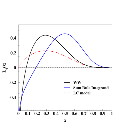
Figure 2: (Color online) Unintegrated OAM for the $u$ quark calculated in the Wandzura Wilczek approximation Eq.(33), compared to the integrand in Ji’s sum rule, Eq.(28), evaluated using the reggeized diquark model of Refs.GGL ; GGL_FF . Results are compared to ${\cal L}_{u}$ obtained using the same input wave functions from Refs.GGL ; GGL_FF in the partonic picture given in Refs.BurkardtBC (labeled LC in the graph).

Next we propose an observable that gives a direct experimental access to the quark OAM. The GPDs contributions to the amplitudes for Deeply Virtual Compton Scattering (DVCS) experiments were computed up to twist three in Refs.BelMuel ; Kivel (see also BelRad ). By referring to the notation of Ref.BelMuel for the CFFs we see that the contribution of $G_{2}$ is found in the singularity free combination given by

$$\widetilde{\mathcal{H}}^{eff}=-2\xi\left(\frac{1}{1+\xi}\widetilde{\mathcal{H}}+\widetilde{\mathcal{H}}^{+}_{3}-\widetilde{\mathcal{H}}^{-}_{3}\right),$$ (34)

where (Table 1),

$$\widetilde{\mathcal{H}} = C^{+}\otimes\widetilde{H},\;\;\;\;\widetilde{\mathcal{H}}_{3}^{+}=C^{+}\otimes\widetilde{E}_{2T}^{\prime},\;\;\;\;\widetilde{\mathcal{H}}_{3}^{-}=C^{-}\otimes\widetilde{E}_{2T},$$ (35)

and,

$$C^{\pm}=-\frac{1}{x-\xi+i\epsilon}\pm\frac{1}{x+\xi-i\epsilon}$$ (36)

In order to extract $G_{2}\equiv\widetilde{E}_{2T}$ from experiment one needs to first of all single out the observables sensitive to $\widetilde{\cal H}^{eff}$. These are the azimuthal asymmetries for DVCS on a longitudinally polarized proton, namely the single spin asymmetry averaged over all beam polarizations, $A_{UL}$, and the double spin asymmetry where both beam and target are polarized, $A_{LL}$. Both $A_{UL}$, and $A_{LL}$ have been recently measured HERMES ; pisano_privcomm .

In this Letter we show our calculation of the twist two and twist three contributions to $A_{UL}$ BelMuel ,

$$A_{UL}=\frac{N_{s_{z}=+}-N_{s_{z}=-}}{N_{s_{z}=+}+N_{s_{z}=-}}$$ (37)

where $N_{s_{z}=\pm}$ is a measure of the number of scatterings on a proton with longitudinal spin, $s_{z}=\pm 1/2$. The dependence of $A_{UL}$ on the the angle $\phi$, or the azimuthal angle between the lepton plane and the plane of the virtual and real photons can be written keeping terms up to twist three as,

$$A_{UL}=\frac{a\sin\phi+b\sin 2\phi}{c_{0}+c_{1}\cos\phi+c_{2}\cos 2\phi}$$ (38)

where the coefficients for the total unpolarized cross section in the denominator, $c_{0}$, $c_{1}$, and $c_{2}$ are given by combinations of the Bethe-Heitler (BH), DVCS, and BH-DVCS interference terms BelMuel . The coefficients in the numerator, also displayed in BelMuel contain the GPDs of interest in our study namely,

$$a\approx s^{\mathcal{I}}_{1,LP}\propto F_{1}(t)\Im m\widetilde{\mathcal{H}}$$

and

$$b\approx s^{\mathcal{I}}_{2,LP}\propto F_{1}(t)\Im m\widetilde{\mathcal{H}}^{eff},$$

where $F_{1}(t)$ is the Dirac form factor.

In Fig.3 we show the asymmetry values plotted vs. the momentum transfer squared $-t$, compared to HERMES data HERMES at the Bjorken $x$ and scale $Q^{2}$ of the data. Both the twist two ($\sin\phi$) and twist three ($\sin 2\phi$) modulations are shown. The blue bands represent the predictions from the GPD model of GGL ; GGL_FF including the error from the model’s parameters variations calculated in WW approximation. As we can see from the figure the $\sin 2\phi$ modulation, dominated by the $\tilde{\cal H}$ Compton form factor, is sizable: an extraction of $G_{2}$ is then possible. More accurate data analyses that will allow us to better single out this term will be available soon pisano_privcomm .

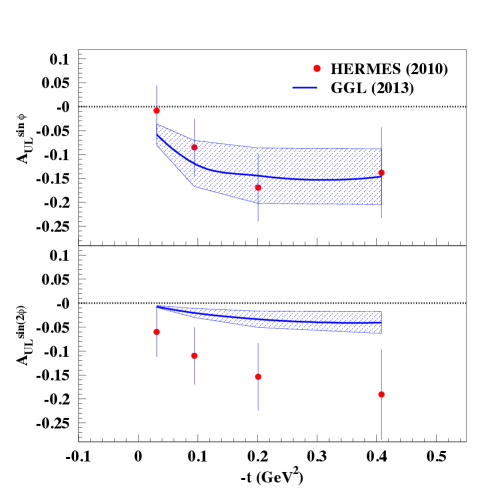
Figure 3: (Color online) The asymmetry $A_{UL}$ twist two ($\sin\phi$) and twist three ($\sin 2\phi$) modulations plotted vs. the momentum transfer squared $-t$, compared to HERMES data HERMES at the Bjorken $x$ and scale $Q^{2}$ of the data. The blue bands represent the predictions from the GPD model of GGL ; GGL_FF denoted by GGL in the legend, including the error from the model’s parameters variations calculated in WW approximation.

Finally, we notice that, as shown recently in Hatta , both the canonical JM_SR and Ji’s OAM admit the same WW approximated form, while their genuine twist three contributions differ.

5. In conclusion, we have proposed the first experimental access to the quark OAM, through twist three GPDs. With the corresponding data from HERMES and the soon available data from JLab, $L_{q}$ could be extracted.

Our suggestion for a direct OAM measurement originates from an interpretation of the helicity structure of GTMDs and GPDs that identifies the relevant spin projections for this quantity. In particular we show that OAM is determined by a transverse spin correlation at twist three.

The non-zero $F_{14},G_{11}$ cannot directly be related to the single longitudinal polarizations of either the quarks or the nucleons within the transverse momentum distributions, and final state interactions should be introduced. Efforts to extract dynamical information from model calculations of these will lead to deceptive results. Because the quarks are off their mass shell before imposing any particular model, the counting of independent helicity amplitudes is complicated leading to a doubling of the number of helicity states FGM . Starting from this observation we proposed a QCD approach where: 1) single longitudinal polarizations observables can be derived; 2) they involve twist three distributions. Our approach is complementary to the one in Ref.Burkardt_torque that was derived using TMD factorization.

Our most important result is perhaps in dispelling the notion that what is believed to be the orbital angular momentum component of the nucleon spin sum rule cannot be observed directly in hard scattering experiments. Both the JM and Ji decompositions correspond to twist three contributions, and their validity can be tested by measuring twist three GPDs. These observables can be obtained from both HERMES data HERMES and in forthcoming Jefferson Lab analyses pisano_privcomm .

We are grateful to Silvia Pisano for fruitful discussions as well as information about the DVCS observables. This work was funded in part by the Belgian Fund F.R.S.-FNRS via the contract of Charge de recherches (A.C.), and by U.S. D.O.E. grant DE-FG02-01ER4120 (S.L., A.R.). A.R. thanks the INFN Laboratori Nazionali di Frascati for support.

References

• (1) M. Burkardt, Phys. Rev. D 66, 114005 (2002)
• (2) S. Meissner, A. Metz and K. Goeke, Phys. Rev. D 76, 034002 (2007)
• (3) S. Meissner, A. Metz and M. Schlegel, JHEP 0908, 056 (2009)
• (4) D. E. Soper, Phys. Rev. D 15, 1141 (1977).
• (5) S. Scopetta and V. Vento, Phys. Lett. B 460, 8 (1999) [Erratum-ibid. B 474, 235 (2000)]
• (6) S. J. Brodsky, D. S. Hwang, B. -Q. Ma and I. Schmidt, Nucl. Phys. B 593, 311 (2001)
• (7) C. Lorce and B. Pasquini, Phys. Rev. D 84, 014015 (2011) [arXiv:1106.0139 [hep-ph]].
• (8) C. Lorce, B. Pasquini, X. Xiong and F. Yuan, Phys. Rev. D 85, 114006 (2012)
• (9) X. Ji, X. Xiong and F. Yuan, Phys. Rev. Lett.  109, 152005 (2012)
• (10) D. Sivers, Phys. Rev. D 41, 83 (1990).
• (11) H. Avakian, A. V. Efremov, P. Schweitzer and F. Yuan, Phys. Rev. D 78, 114024 (2008)
• (12) J. She, J. Zhu and B. -Q. Ma, Phys. Rev. D 79, 054008 (2009)
• (13) D.V. Kiptily and M.V. Polyakov, Eur. Phys. J. C. 37, 105 (2004).
• (14) M. Penttinen, M. V. Polyakov, A. G. Shuvaev and M. Strikman, Phys. Lett. B 491, 96 (2000)
• (15) Y. Hatta, Phys. Lett. B 708, 186 (2012); Y. Hatta and S. Yoshida, JHEP 1210, 080 (2012)
• (16) A. V. Belitsky, D. Mueller and A. Kirchner, Nucl. Phys. B 629, 323 (2002)
• (17) A. Airapetian et al. [HERMES Collaboration], JHEP 1006, 019 (2010)
• (18) S. Pisano and H. Avakian, private communication.
• (19) G. R. Goldstein, J. O. Hernandez and S. Liuti, Phys. Rev. D 84, 034007 (2011)
• (20) J. O. Gonzalez-Hernandez, S. Liuti, G. R. Goldstein and K. Kathuria, arXiv:1206.1876 [hep-ph].
• (21) M. Jacob and G.C. Wick, Ann. Phys. 7, 404 (1959).
• (22) H.A. Fearing, G.R. Goldstein and M.J. Moravcsik, Phys. Rev. D29, 2619 (1984).
• (23) M. Diehl, Eur. Phys. J. C 25, 223 (2002).
• (24) R.K. Ellis, W. Furmanski and R. Petronzio, Nucl. Phys. B 212, 29 (1983).
• (25) J. D. Jackson, G. G. Ross and R. G. Roberts, Phys. Lett. B 226, 159 (1989).
• (26) S. Liuti, A. Courtoy, G. R. Goldstein, J. O. G. Hernandez and A. Rajan, arXiv:1309.7029 [hep-ph], to be published in Proceedings of QCD workshop.
• (27) A. Courtoy, G.Goldstein, O. Gonzalez, S. Liuti and A. Rajan, in preparation.
• (28) J. B. Kogut and D. E. Soper, Phys. Rev. D 1, 2901 (1970).
• (29) R. L. Jaffe, In *Erice 1995, The spin structure of the nucleon* 42-129 [hep-ph/9602236].
• (30) N. Kivel, M. V. Polyakov and M. Vanderhaeghen, Phys. Rev. D 63, 114014 (2001)
• (31) R. L. Jaffe and A. Manohar, Nucl. Phys. B 337, 509 (1990).
• (32) X. -D. Ji, Phys. Rev. Lett.  78, 610 (1997)
• (33) M. Burkardt, Phys. Rev. D 88, 014014 (2013)
• (34) A. Harindranath and R. Kundu, Phys. Rev. D 59, 116013 (1999)
• (35) M. Burkardt and H. BC, Phys. Rev. D 79, 071501 (2009)
• (36) A. V. Belitsky and A. V. Radyushkin, Phys. Rept.  418, 1 (2005)
• (37) M. Wakamatsu, Phys. Rev. D 85, 114039 (2012)