A Non-radial Oscillation Mode in an Accreting Millisecond Pulsar?

Abstract

We present results of targeted searches for signatures of non-radial oscillation modes (such as r- and g-modes) in neutron stars using RXTE data from several accreting millisecond X-ray pulsars (AMXPs). We search for potentially coherent signals in the neutron star rest frame by first removing the phase delays associated with the star’s binary motion and computing FFT power spectra of continuous light curves with up to $2^{30}$ time bins. We search a range of frequencies in which both r- and g-modes are theoretically expected to reside. Using data from the discovery outburst of the 435 Hz pulsar XTE J1751$-$305 we find a single candidate, coherent oscillation with a frequency of $0.5727597\times\nu_{spin}=249.332609$ Hz, and a fractional Fourier amplitude of $7.46\times 10^{-4}$. We estimate the significance of this feature at the $1.6\times 10^{-3}$ level, slightly better than a $3\sigma$ detection. Based on the observed frequency we argue that possible mode identifications include rotationally-modified g-modes associated with either a helium-rich surface layer or a density discontinuity due to electron captures on hydrogen in the accreted ocean. In the latter case the presence of sufficient hydrogen in this ultracompact system with a likely helium-rich donor would present an interesting puzzle. Alternatively, the frequency could be identified with that of an inertial mode or a core r-mode modified by the presence of a solid crust, however, the r-mode amplitude required to account for the observed modulation amplitude would induce a large spin-down rate inconsistent with the observed pulse timing measurements. For the AMXPs XTE J1814$-$338 and NGC 6440 X-2 we do not find any candidate oscillation signals, and we place upper limits on the fractional Fourier amplitude of any coherent oscillations in our frequency search range of $7.8\times 10^{-4}$ and $5.6\times 10^{-3}$, respectively. We briefly discuss the prospects and sensitivity for similar searches with future, larger X-ray collecting area missions.

1. Introduction

The study of global stellar oscillations can provide a powerful probe of the interior properties of stars. A prime example of this is the rich field of helioseismology. By comparison, efforts to probe the exotic interiors of neutron stars via similar methods are still in their infancy, but recent observational results have provided new impetus to further explore asteroseismology of neutron stars. For example, observations of quasiperiodic oscillations (QPOs) in the X-ray flux of highly magnetized neutron stars, “magnetars” (Duncan, 1998; Israel et al., 2005; Strohmayer & Watts, 2005, 2006; Watts & Strohmayer, 2006; Woods & Thompson, 2006), which have been linked to global torsional vibrations within the star’s crust, may ultimately provide a promising new probe of a neutron star’s internal composition and structure. In addition to the magnetar QPOs, burst oscillations, pulsations seen at or near the neutron star spin frequency during thermonuclear X-ray bursts from accreting, low mass X-ray binary (LMXB) neutron stars (see Strohmayer & Bildsten (2006); Watts (2012) for reviews on burst oscillations), may also be linked to stellar pulsations. Although a comprehensive understanding of the physics of these oscillations is still being developed, one of the models that has been proposed to explain them is the Rossby wave (r-mode) model, which assumes that the oscillation is produced by a low-frequency r-mode (Rossby wave) propagating in the neutron star surface “ocean.” In this case the r-mode modulates the temperature distribution across the neutron star surface and the resulting angular variations of the surface thermal emission–combined with the spin of the star–produce pulsations in the X-ray flux observed from the stellar surface. For example, Lee & Strohmayer (2005) and Heyl (2005) have explored this model, and computed light curves for small azimuthal wavenumber, $m$, surface r-modes on rotating neutron stars.

Accretion-powered millisecond X-ray pulsars (AMXPs) also show small-amplitude X-ray oscillations with periods equal to their spin periods. To explain the low modulation amplitudes and nearly sinusoidal waveforms in these sources, Lamb et al. (2009) proposed a model in which the X-rays are emitted from a hot-spot that is located at or near a magnetic pole of the star, and the magnetic pole is assumed to be close to the spin axis of the star. When the emitting region is close to the spin axis, a small variation in its position can produce relatively large changes in the amplitude and phase of the X-ray variations. Lee (2010) and Numata & Lee (2010) later suggested that global oscillations of neutron stars (for example, r-modes) can periodically perturb such a hot-spot and therefore the oscillation mode periods might potentially be observable as X-ray flux oscillations from these sources (we discuss this in more detail below).

The global oscillation spectrum of neutron stars is rich, and has been classified according to the restoring force relevant to each particular mode (McDermott et al., 1988). For example, pressure modes (p-modes and the f-mode) are primarily supported by internal pressure fluctuations (essentially sound waves) in the star and have frequencies in the $10$ kHz range that scale as $(\bar{\rho})^{1/2}$, where $\bar{\rho}$ is the stellar mean density. The successive overtones of these modes have higher frequencies. By overtones we mean modes with an increasing number of nodes (zero crossings) in their radial displacement eigenfunctions. Gravity modes (g-modes) confined primarily to the region above the solid crust have buoyancy as their restoring force and frequencies in the $1-100$ Hz range (in the slow-rotation limit). The overtones of these surface g-modes have decreasing frequencies. The finite shear modulus of the neutron star crust leads to additional, shear-dominated modes. These include the purely transverse torsional modes (t-modes), briefly mentioned above in the context of magnetar QPOs, which have frequencies larger than about $30$ Hz, and the s-modes, which possess both radial and transverse displacements. For both classes of torsional modes the overtones–whose radial eigenfunctions have at least one node in the crust–can be thought of as shear waves traveling vertically through the crust. They have frequencies in the kHz range that scale inversely with the thickness of the neutron star crust.

In the case of rotating neutron stars another important class of oscillations are the so-called inertial modes for which the restoring force of the pulsations is provided by the Coriolis force (Yoshida & Lee, 2000a, b). A well known sub-set of these are the r-modes that couple to gravitational radiation and can be driven unstable by the Chandrasekhar-Friedman-Schutz (CFS) mechanism (Friedman & Schutz, 1978; Andersson, 1998; Friedman & Morsink, 1998). Whether they are excited or not is a competition between the driving due to the coupling to gravitational radiation and the various mechanisms–such as bulk and shear viscosity–that can damp the oscillations. The damping and transport properties, such as viscosity, heat conductivity and neutrino emissivity, depend significantly on the phase of dense matter present in the star, and since r-modes can both brake the star’s rotation and heat its interior, study of the spin and thermal evolution of neutron stars can be a potentially important probe of the dense matter interior (Mahmoodifar & Strohmayer, 2013; Haskell et al., 2012). Moreover, the co-rotating frame r-mode frequencies depend on the stellar spin rate and the internal composition and structure of the star (Lindblom et al., 1999; Yoshida & Lee, 2000b; Alford et al., 2012). Thus, observations of the frequencies of non-radial oscillation modes of neutron stars would be very useful in probing their internal structure, but except for the magnetar QPOs linked to crustal vibrations and perhaps the surface r-modes linked with burst oscillations, there have been no other direct observations of these oscillations.

It is relevant to ask the question of how the presence of non-radial oscillations might be inferred from observations. As noted briefly above in the context of burst oscillations, if an r-mode modulates the temperature distribution across the neutron star surface, then this may be revealed as a pulsation in the X-ray flux from the star. Another possibility is that surface motions induced by a particular oscillation mode perturb the X-ray emitting hot-spot that is present during the outbursts of accreting millisecond X-ray pulsars (AMXPs). This mechanism seems most relevant for quasi-toroidal modes (such as the r- and g-modes) in which the dominant motions are transverse–locally parallel to the stellar surface–as opposed to radial. Such transverse motions can deform an emitting region in a periodic fashion and thus imprint the periodic deformation on the observed light curve from the source. Indeed, Numata & Lee (2010) explored this mechanism, and computed the resulting light curves from such a perturbed hot-spot on a rotating neutron star. Since the hot-spot rotates with the star it is periodically deformed at the oscillation frequency of the mode as measured in the co-rotating frame of the star. They computed the modulation that would be produced by a hot-spot that is perturbed by the surface motions associated with a global r-mode, and showed that the r-mode frequency specified in the co-rotating frame is imprinted on the light curve seen by a distant observer. We note that surface g-modes also have dominant horizontal displacements and could also be relevant in this context. Using this model they also demonstrated that the observed modulation amplitude of the light curve could be used to infer or constrain the mode amplitude.

In the limit of slow rotation it is well known that the r-mode frequency in the co-rotating frame is given by $\omega=2m\Omega/l(l+1)$, where $m$ and $l$ are the spherical harmonic indices that describe the angular distribution of the dominant toroidal displacement vector, and $\Omega$ is the stellar spin frequency. The most unstable r-mode is that associated with $l=m=2$, which has the familiar frequency $\omega=2\Omega/3$ in the co-rotating frame. For more rapidly rotating neutron stars, like the AMXPs, the r-mode frequency deviates from the above limit and is typically calculated in an expansion in powers of the angular rotation frequency (see, for example, Lockitch & Friedman (1999); Yoshida & Lee (2000b); Lindblom et al. (1998); Alford et al. (2012)). This leads to an expression for $\omega$ of the form, $\omega=\Omega(\kappa_{0}+\kappa_{2}\bar{\Omega}^{2})$, where for the $l=m=2$ r-mode, $\kappa_{0}=2/3$, $\bar{\Omega}^{2}=\Omega^{2}(R^{3}/GM)$ and $\kappa_{2}$, which represents the next-order correction to the r-mode frequency, depends on the properties of the unperturbed stellar model, such as its equation of state (EOS) and entropy stratification (Yoshida & Lee, 2000b; Alford et al., 2012). Thus, if an r-mode frequency is detected it can potentially provide interesting information about the stellar interior, and perhaps be used to identify the dense matter phase present in the core (see, for example, Figure 3 in Alford et al. 2012).

The above discussion ignores the effects that the solid crust of the neutron star may have in modifying the r-modes and their surface displacements. For example, Yoshida & Lee (2001) have investigated the r-modes for neutron star models including a solid crust and show that they are strongly influenced by mode coupling with the crustal torsional modes (t-modes). They found that this mode coupling can reduce the r-mode frequency from $2\Omega/3$ to values as low as $\Omega/2$ to $2\Omega/5$ (see their Figure 2), and the reduction occurs at and above a critical rotational frequency that is close to the fundamental torsional mode frequency (we discuss this in more detail below).

Since the spin frequency of outbursting AMXPs can be tracked with high precision, and the r-mode frequencies are computed as a series expansion in powers of the spin frequency, it is possible to carry out coherent, targeted searches in such sources for r-modes in a specific range of frequencies both above and below its “expected” ($\Omega\rightarrow 0$ limit) value, $2\Omega/3$. Similar arguments apply for other modes as well, such as the surface g-modes, some of which have frequencies that overlap the expected frequency range for the r-modes. Here we present the results of power spectral searches for the signatures of such modes using data from several AMXPs obtained with the Rossi X-ray Timing Explorer (RXTE). It is not our intent here to present an exhaustive search of all known AMXPs, rather, we illustrate the methods and present results for three sources; XTE J1751$-$305 (hereafter J1751), XTE J1814$-$338 (hereafter J1814), and NGC 6440 X-2 (hereafter X-2), all of which are within the nominal r-mode instability window computed for hadronic matter, and which had the highest inferred r-mode amplitude upper limits in our recent study (Mahmoodifar & Strohmayer, 2013). We will present a study of additional sources, including SAX J1808.4$-$3658, in a sequel. The paper is organized as follows. In §2 we illustrate in some detail our search analysis procedures using data from the 435 Hz AMXP J1751. We also present the search results for this source and describe our best detection candidate, which is at a frequency of $0.57276\nu_{spin}$ (249.33 Hz). In §3 we summarize our search results for the additional targets, the 206 Hz pulsar X-2, and the 314 Hz pulsar J1814. In §4 we discuss possible mode identifications for the best candidate frequency in J1751. We also briefly discuss how future observations with larger collecting area missions, such as ESA’s Large Observatory for X-ray Timing (LOFT, Feroci et al. (2012)), and the Advanced X-ray Timing Array (AXTAR, Ray et al. (2010)) can improve the sensitivity of such searches. We conclude with a brief summary of our findings in §5.

2. A Coherent Search in XTE J1751$-$305

The most sensitive search procedure for a particular timing signature, such as a coherent pulsation, depends on the nature of that signature. In the context of searches employing Fourier power spectra the greatest sensitivity is achieved by matching the frequency resolution of the power spectrum to the expected frequency bandwidth of the signal. Thus, for a highly coherent signal the greatest sensitivity is achieved by maximizing the frequency resolution. This effectively means that one should compute a single Fourier power spectrum of the longest time series obtainable from the available data. While the exact frequency bandwidth of a candidate signal is often not known precisely, the work of Numata & Lee (2010) suggests that a signal produced by perturbation of a hot-spot by an r-mode (or some other non-radial mode) may be quite coherent. On the other hand, conditions in the neutron star surface layers can evolve as accretion continues during an outburst and these sources are known to exhibit timing noise that is likely associated with variations in the latitude and azimuth of the accretion hot-spot (Patruno et al., 2009), so such processes are likely to limit the effective coherence of such signals. Because of this, as well as computational constraints, we restrict the size of the longest light curves for Fourier analysis in this work to $N=2^{30}$ time bins. For a sample rate of 2048 Hz this corresponds to a time interval of 524,288 s, or about 6 days. Depending on the amount of data present for a given source, one can then average several independent power spectra and/or adjacent Fourier frequency bins to search for signals with broader frequency bandwidths (such as quasi-periodic oscillations, QPOs).

In order to carry out searches at the highest frequency resolution it is necessary to remove as best as possible the frequency drifts associated with the binary motion of the neutron star about the center of mass of the system in which it resides. This effectively places the observer at the center of mass of the binary system, a point from which the neutron star is neither approaching nor receding. These considerations lead to the following basic steps we use to carry out a search. First, the X-ray event arrival times are corrected to the Solar System barycenter. Next, we fit a model to the observed orbit-induced phase variations. This orbit model is used to convert each photon event arrival time to a neutron star rotation phase. These phases are then converted back to fiducial times using the best-determined spin frequency of the neutron star. Finally, these orbit corrected times can be used to compute a single light curve which can then be Fourier analyzed using Fast Fourier Transform (FFT) power spectral methods.

To illustrate the procedure in some detail we step through our analysis for J1751. This source was discovered in early April, 2002 during regular monitoring observations of the Galactic center region using the RXTE Proportional Counter Array (PCA, Markwardt et al. (2002)). The outburst was relatively short, lasting only about 10 days. Timing of the X-ray pulsations revealed an ultra-compact system with an orbital period of 42.4 min (Markwardt et al., 2002). For our coherent search we used data spanning about 6 days during the peak of the outburst. Figure 1 shows the source light curve sampled in 2 s bins. We used PCA event mode data with a resolution of 125 $\mu$-sec for our study and included all events in the full energy band-pass of the PCA and from all operating detectors. We used the FTOOL faxbary to correct the photon arrival times to the Solar System barycenter. We then applied the orbit timing solution from Markwardt et al. (2002, 2007) (see Table 1 in their 2007 paper) to convert the arrival times to neutron star rotational phases. Figure 2 shows a dynamic power spectrum from a single RXTE orbit, which reveals the time evolution of the pulsar frequency due to the neutron star’s orbital motion. The best fitting orbit model for this time interval (thick solid curve) is also plotted, showing that it accurately predicts the observed evolution. Figure 3 shows the resulting phase residuals after application of the orbit model to the light curve used for our coherent search. The remaining variations are consistent with poisson errors in the phases.

We then used the orbit model to convert each arrival time to a rotational phase. These phases can then be expressed as fiducial times by multiplying by the best-fit pulsar spin period. We use the resulting times to produce a light curve sampled at 2048 Hz that contains $2^{30}=1,073,741,824$ time bins. Finally, we compute an FFT power spectrum of this light curve. The resulting power spectrum has a little more than half a billion frequency bins and a Nyquist frequency of 1024 Hz, thus, simply from file size considerations it is not practical to present a plot of the entire spectrum. However, to demonstrate that the coherent pulsar signal is strongly detected we show in Figure 4 the power spectrum in a narrow frequency band centered on the pulsar signal. Here, the units on the x-axis are $(\sigma/\Omega-1)\times 10^{5}$, where $\sigma$ is a Fourier frequency. Thus, the pulsar signal appears at zero in these units. Moreover, in order to enable direct comparison with the light curve computations of Numata & Lee (2010), see for example their Figure 6, we plot the power spectrum in units of fractional Fourier amplitudes $\sqrt{(a_{j}^{*}a_{j})/N_{tot}}$, where the $a_{j}$ are the complex Fourier amplitudes at Fourier frequency $\nu_{j}=j/(524,288\;s)$, $j$ ranges from $0$ to $2^{29}$, $N_{tot}=44,316,997$ is the total number of events in the light curve, and the $*$ symbol indicates complex conjugation. To convert the fractional Fourier amplitudes to the commonly used Leahy normalization one simply squares the fractional amplitudes, and then multiplies by $2\times N_{tot}$. The commonly employed fractional rms amplitude is simply $\sqrt{2}$ times the fractional Fourier amplitude defined above.

2.1. Search for Co-rotating Frame Frequencies Consistent with r- and g-modes

As noted in §1 above, when a pulsation mode periodically perturbs an X-ray emitting hot-spot that is fixed in the rotating frame of the star, the co-rotating frame mode frequency is imprinted on the light curve seen by a distant observer. Further, rapid rotation tends to increase the co-rotating frame frequency of the $l=m=2$ r-mode from the slow-rotation limit of $\omega=2\Omega/3$, while the influence of a solid crust may decrease it. Based on the discussion above, a reasonable frequency range to search is then $2/3-k_{1}\leq\omega/\Omega\leq(2/3+k_{2})$, where $k_{1}$ represents a plausible reduction in the frequency based on the possible crustal effects to the r-mode, and $k_{2}$ represents a reasonable maximum increase for $\kappa_{2}\bar{\Omega}$ given the observed spin frequency of J1751 and various possible masses, equations of state and interior compositions for the neutron star. Based on the calculations of Yoshida & Lee (2001) and Alford et al. (2012, see their Figure 3), plausible values for $k_{1}$ and $k_{2}$ are 0.25 and 0.09, respectively. This defines a search range from $0.4166\leq\omega/\Omega\leq 0.75667$. A search in that range reveals one candidate peak in slightly more than 77.59 million independent Fourier frequency bins. Figure 5 shows a portion of the full-resolution spectrum in the vicinity of this peak. It appears at a frequency of $0.5727597\times\nu_{spin}=249.332609$ Hz, and has a fractional Fourier amplitude of $7.455\times 10^{-4}$.

To assess the significance of this peak we first convert its fractional Fourier amplitude to a Leahy-normalized power and then estimate its single-trial probability using the expected noise power distribution, which for a single power spectrum is the $\chi^{2}$ distribution with 2 degrees of freedom. The peak Leahy-normalized power is then 49.26, which corresponds to a single-trial probability of $2\times 10^{-11}$. Accounting for the number of trials by multiplying by the number of independent Fourier frequencies in the search range, $77.6\times 10^{6}$, gives a significance of $1.6\times 10^{-3}$, which is a little better than a $3\sigma$ detection. We then used a portion of the power spectrum at higher frequencies (from 1.6 to 2.2 times the pulsar spin frequency) to investigate how accurately the distribution of noise powers follows the expected $\chi^{2}$ distribution. The result is shown in Figure 6, where the red dashed line denotes the probability to exceed a given Fourier power for the $\chi^{2}$ distribution with 2 degrees of freedom, and the Leahy-normalized power spectral data are plotted as a histogram. Over the range of Fourier powers present in the data the power spectral values show a good match to the expected distribution. The Fourier power of the candidate peak is marked by the vertical dashed-dot line, and as indicated above, has a single trial probability of $2\times 10^{-11}$. Based on this we think our significance estimate is reasonable.

We next averaged the full resolution power spectrum in order to search for any broader bandwidth signals that might be present. Figure 7 shows two such averaged power spectra over the full frequency range. The black and green histograms have frequency resolutions of 1/2048, and 1/128 Hz, respectively. The pulsar signal is still easily detected in each case, but we do not find any other significant features at these or other frequency resolutions. The horizontal dashed line marks the amplitude of the candidate signal at $249.33$ Hz discussed above. We can place upper limits on any signal power in our defined search range at these frequency resolutions of $1.64\times 10^{-4}$ and $1.42\times 10^{-4}$, respectively. The horizontal, red dashed line in Figure 7 marks an amplitude given by $1/(N_{tot})^{1/2}=1.50\times 10^{-4}$, which gives a reasonably close approximation to the quoted upper limits for broader band signals.

2.2. Search for Modulation at the Inertial Frame r-mode Frequency

As discussed in §1, if an oscillation mode modulates emission over the entire neutron star surface rather than simply perturbing a hot-spot fixed in the co-rotating frame, then one would expect a pulsation signal at the mode’s inertial frame frequency, $\omega_{i}=2\Omega-\omega$, where $\omega$ is the co-rotating frame frequency. Thus, to search the range of inertial frame frequencies corresponding to the range of co-rotating frame frequencies just discussed in §2.1 we need to search the frequency range $2-(2/3+0.09)<\sigma/\Omega<2-(2/3-0.25)$, which reduces to $1.243<\sigma/\Omega<1.583$. A search reveals no significant peaks in this range. The highest peak appears at a frequency of $1.565327\nu_{spin}$, with a fractional Fourier amplitude limit of $6.6\times 10^{-4}$.

3. Coherent Searches in XTE J1814$-$338 and NGC 6440 X-2

Here we briefly summarize search results for J1814 and X-2.

3.1. Results for XTE J1814$-$338

J1814 was discovered by RXTE in June 2003 using data obtained with the Galactic bulge monitoring program then being conducted with the PCA onboard RXTE. The pulsar has a 314.36 Hz spin frequency and an orbital period of 4.275 hr (Markwardt et al., 2003; Papitto et al., 2007). The discovery outburst lasted for $\approx 50$ days. This object was the first neutron star to exhibit burst oscillations with a significant first harmonic (Strohmayer et al., 2003), and indeed, the persistent pulse profile also shows substantial harmonic content. This source is also known to exhibit significant timing noise, that is, systematic timing residuals remain after modeling the binary Doppler delays (Papitto et al., 2007; Watts et al., 2008b). This noise is still not completely understood, but may represent movement of the accretion hot-spot relative to the stellar spin axis as the accretion rate changes during an outburst (Patruno, 2010). Here we use data from the first 12 days for which such variations were less significant (Watts et al., 2008b). We used data beginning on June 5, 2003 at 02:34:20 UTC and constructed two light curves, each sampled at 2048 Hz and with $2^{30}$ time bins. There are a total of $31,361,962$ X-ray events in the two light curves. We first modeled the orbital variations in a similar manner as described above for J1751. Our orbit parameters are consistent with those of Papitto et al. (2007). Figures 8 and 9 show the resulting orbit-corrected phase residuals for the two data segments used to construct our light curves. One can see that the second interval (Figure 9) shows more systematic timing noise than the first interval (Figure 8). We then computed power spectra for each interval in the same manner as described for J1751. We searched the power spectra in the same frequency ranges as described above for J1751 and for each data interval separately as well as the average power spectrum computed from both intervals. We did not find any significant features in the power spectra. Figure 10 shows two average power spectra computed from both intervals, the black and green histograms have been averaged to frequency resolutions of 1/2048, and 1/128 Hz, respectively. The pulsar fundamental and first harmonic are clearly evident (at 1 and 2 in these units). The horizontal dashed line (black) marks the upper limit of $7.8\times 10^{-4}$ on any signal power at the full frequency resolution of the power spectrum. The horizontal dashed (red) line marks an amplitude given by $1/(N_{tot}/2)^{1/2}\approx 2.5\times 10^{-4}$, which again gives a reasonably close approximation to the upper limits for broader band signals.

3.2. Results for NGC 6440 X-2

Pulsations at 205.89 Hz were detected with RXTE from the globular cluster source NGC 6440 X-2 on 30 August, 2009 (Altamirano et al., 2009). On this date the source was observed for a single RXTE orbit, yielding $\approx 3000$ s of exposure, revealing a 57 min orbital period (Altamirano et al., 2010). A subsequent outburst with detectable pulsations was observed with RXTE on 21 March, 2010, for an additional 3 RXTE orbits and 6600 s of exposure. We used all these data in our search. As for J1751, we first barycentered the data using the best determined position from Heinke et al. (2010). Because the available data for this source are too sparse to enable calculation of a single, coherent Fourier power spectrum, we separately modeled the orbital variations in each of the four data segments. We then generated light curves using the orbit-corrected arrival times, computed a Fourier power spectrum for each, and then averaged them. The light curves were sampled at 8192 Hz, yielding a Nyquist frequency of 4096 Hz. The resulting averaged power spectrum is shown in Figure 11. Since there are many fewer Fourier frequencies compared to either J1751 or J1814, we show the spectrum at the full frequency resolution. Two spectra are shown in Figure 11, the black curve is plotted at the full frequency resolution ($3.125\times 10^{-4}$ Hz), and the green curve has been averaged by a factor of 32 to a resolution of 0.01 Hz. The pulsar fundamental is clearly evident (at 1 in these units), but there are no other candidate detections. At these resolutions we can place upper limits on any signal power in our search ranges of $5.6\times 10^{-3}$ (at $3.125\times 10^{-4}$ Hz resolution), and $2.8\times 10^{-3}$ (at $0.02$ Hz). Because much less data is available for X-2 than for either J1751 or J1814, the limits are not as constraining as for those sources.

4. Discussion

As discussed in §2, we found a candidate oscillation at a frequency $\omega=0.5727\Omega$ with an estimated significance of $1.6\times 10^{-3}$ in data from the discovery outburst of J$1751$. Here we discuss possible mode identifications for this candidate oscillation. As mentioned in the introduction, AMXPs show small-amplitude X-ray oscillations with periods equal to the spin period of the star. To explain their low modulation amplitudes and nearly sinusoidal waveforms Lamb et al. (2009) proposed a model in which X-rays are emitted from a hot-spot at the stellar surface and near a magnetic pole that is assumed to be close to the rotation axis of the star. If we assume that this model is correct, then transverse motions induced by the non-radial oscillations at the surface of the star can perturb the hot-spot periodically, and these periodicities might be observable in the radiation flux from the star (Numata & Lee, 2010). In addition to producing X-ray variations by perturbing the hot-spot, if the amplitude of the oscillations at the surface of the star are large enough they might also generate X-ray variations by modulating the surface temperature of the star (Lee & Strohmayer, 2005). In the former case–where the surface oscillation perturbs the hot-spot–since it is co-moving with the star, a distant observer will detect the oscillation frequency of the mode as measured in the co-rotating frame of the star (we refer to this as the “co-rotating frame scenario”). This has been shown by Numata & Lee (2010) for the case of r-modes. On the other hand, oscillation-induced temperature perturbations will produce X-ray variations with the same periodicity as the oscillation frequency of the mode as measured in an inertial frame (we call this the “inertial frame scenario”).

For fast rotating, accreting neutron stars such as J1751 the most relevant restoring forces that can produce stellar pulsations with frequencies that might be consistent with the candidate frequency in J1751 are the coriolis force–due to the star’s rotation–and buoyancy associated with thermal and composition gradients. As briefly summarized in §1, the corresponding oscillation modes associated with these forces are the inertial modes (which includes the r-modes) and the gravity modes (g-modes). In general, both forces are present and the nature of the resulting modes will depend on their relative strength. For example, at high rotation rates the coriolis force will almost certainly dominate–except perhaps within a very small band around the rotational equator–and the resulting pulsation modes are expected to be inertial in character. At the other extreme of slow rotation buoyancy can eventually prevail resulting in essentially pure g-modes (Yoshida & Lee, 2000b; Passamonti et al., 2009). Other oscillation modes such as crustal toroidal modes associated with the finite shear modulus of the crust, or f- and p-modes due to pressure forces are either confined to the crust or core of the star and may not be able to induce motions at the surface, or they have higher frequencies which are inconsistent with the candidate oscillation. In what follows we discuss how the candidate frequency in J$1751$ might be identified as a surface g-mode, a core r-mode, or perhaps an inertial mode in a fast rotating star.

4.1. g-modes

As briefly mentioned above, the g-modes are low frequency non-radial oscillation modes of neutron stars with buoyancy as their restoring force. In a 3 component NS model composed of a fluid core, a solid crust and a fluid ocean, g-modes might be excited in the core and/or in the ocean, but the finite shear modulus excludes them from the crust (Bildsten & Cutler, 1995). As a result core g-modes are unlikely to have observable effects on the radiation observed from the surface of the star. Therefore, here we focus on the surface g-modes that are confined to a thin layer at the surface of the star. There have been many studies on g-modes in neutron stars (McDermott & Taam, 1987; Strohmayer & Lee, 1996; Bildsten & Cutler, 1995; Bildsten et al., 1996; Bildsten & Cumming, 1998). We are particularly interested in the surface g-modes in AMXPs. The conditions at the surface of these objects evolve slowly due to the accretion and their g-mode spectrum is different from that of the isolated and non-accreting neutron stars. The g-modes at the surface of an accreting NS can be divided into several different categories according to their different sources of buoyancy, such as an entropy gradient or density discontinuity. Bildsten & Cutler (1995) studied surface g-modes in accreting systems with thermal buoyancy as the restoring force. They obtained an analytic result for the mode frequency in the non-rotating limit ($\Omega\rightarrow 0$)

$$f_{th} =6.26Hz\left(T_{8}\frac{16}{A}\right)^{\frac{1}{2}}\left(1+\left(\frac{3n\pi}{2\ln(\rho_{b}/\rho_{t})}\right)^{2}\right)^{-1/2}$$

$$\times\left(\frac{10km}{R}\right)\left(\frac{l(l+1)}{2}\right)^{\frac{1}{2}},$$ (1)

where $T_{8}=\frac{T}{10^{8}K}$, $A$ is the mass number, $l$ is the spherical harmonic index, $n$ is the number of radial nodes in the displacement eigenfunction, $R$ is the stellar radius, and $\rho_{b}$ and $\rho_{t}$ are densities at the bottom and top of the ocean, respectively. Strohmayer & Lee (1996) studied thermal g-modes in a steady state accreting and nuclear burning atmosphere, and found some modes can be excited by the $\epsilon$ mechanism (perturbations in the nuclear burning). For example, see their Table 3 for results on the oscillation periods of $g_{1}$ and $g_{2}$ modes. Bildsten & Cumming (1998) studied the effect of hydrogen electron captures on g-modes in the ocean of accreting neutron stars. They found that the sudden increase in the density at the hydrogen electron capture layer supports a density discontinuity mode with a non-rotating limit frequency

$$f_{d}\approx 35Hz\left(\frac{X_{r}}{0.1}\right)^{\frac{1}{2}}\left(1-\frac{\Delta Z}{\Delta A}\right)^{\frac{1}{2}}\left(\frac{10km}{R}\right)\left(\frac{l(l+1)}{2}\right)^{\frac{1}{2}},$$ (2)

where $X_{r}$ is the residual mass fraction of hydrogen, and $\Delta Z$ and $\Delta A$ are the changes in the charge and mass of the nuclei from one side of the discontinuity to the other.

Piro & Bildsten (2004) studied non-radial oscillations at the surface of a helium burning neutron star. They found one unstable mode that resides in the helium atmosphere and is supported by the buoyancy of the helium/carbon interface. The frequency of this mode in the non-rotating limit is given by

$$f_{th-He}\approx(20-30Hz)\sqrt{\frac{l(l+1)}{2}},$$ (3)

which depends on the accretion rate. Similarly to the results of Strohmayer & Lee (1996), they find that this mode can also be driven unstable by the $\epsilon$-mechanism, and they also compute results for higher accretion rates. Now, the orbital period of J$1751$ is very short ($\sim 42$ min) (Markwardt et al., 2002), which means that it is a very compact system and thus the donor star is likely a helium white dwarf. This suggests that the accreted material is helium-rich and it therefore seems plausible that the system might show the unstable shallow surface waves that are obtained for a helium atmosphere.

It is important to note that the g-mode frequencies just discussed are obtained in the non-rotating limit $(\Omega\rightarrow 0)$ and, as alluded to above, they will be modified by rapid rotation of the star. Bildsten et al. (1996) studied the effect of high spin frequencies on the g-mode spectrum in the so-called “traditional approximation,” in which mode propagation is confined to a thin shell, the radial component of the coriolis force is neglected, and the radial displacements produced by the modes are assumed to be much less than the horizontal displacements. These approximations are reasonable for surface g-modes as long as the coriolis force remains less than the buoyant force (see §2 of Bildsten et al. (1996)). This condition can be expressed as, $N^{2}\gg(\Omega\omega R)/h$, where $N$, $R$ and $h$ are the Brunt Väisällä frequency (which sets the strength of buoyancy), stellar radius, and characteristic scale height in the surface envelope, respectively. Assuming the candidate frequency in J1751 represents the mode frequency in the co-rotating frame (and using the 435 Hz spin frequency of J1751), then $\omega=0.573\Omega$, and we would require $N^{2}\gg 4.3\times 10^{6}(R/h)$ Hz².

From this analysis Bildsten et al. (1996) found that stellar rotation “squeezes” the eigenfunctions toward the equator within an angle $\cos\theta<\frac{1}{q}$ where $\theta$ is measured from the pole, $q=\frac{2\Omega}{\omega}$, and the oscillation frequency of the mode (in the co-rotating frame) in a non-rotating star, $\omega_{l,0}$, is related to the mode frequency at arbitrary spin frequencies by the following equation

$$\omega^{2}=2\Omega\omega_{l,0}\left[\frac{(2l_{\mu}-1)^{2}}{l(l+1)}\right]^{1/2}$$ (4)

where $l_{\mu}$ is the number of zero crossings in the angular displacement between $\cos\theta=-\frac{1}{q}$ and $+\frac{1}{q}$. Thus, the surface displacements of the rotationally modified g-modes are strongly confined to the equatorial region at high spin frequencies and the modes are exponentially damped for $\cos\theta\geq 1/q$ (Bildsten et al., 1996). For the spin frequency of J1751, $q\simeq 3.5$ (assuming that the 249.33 Hz candidate frequency is associated with a co-rotating frame mode frequency). This leaves open the question of what mode amplitudes would be needed to effectively perturb a hot-spot located near the rotational pole.

Moreover, the relevant scale height, $h$, will depend on details of the surface envelopes in question, however, a typical value for the He-rich envelopes of Piro & Bildsten (2004) is $h\approx 200$ cm, thus, for a 10 km radius neutron star we would require $N^{2}\gg 2.2\times 10^{10}$ Hz² in order to satisfy the assumptions associated with the traditional approximation. We note that this condition appears to be technically violated for these envelopes as $N$ is everywhere less than about $1\times 10^{5}$ Hz (see their Figures 2 and 3). This suggests the need for more theoretical work in order to more accurately determine the surface g-mode properties for rotation rates appropriate to the faster spinning AMXPs (such as J1751). In addition, more work similar to that done in the context of r-modes by Numata & Lee (2010) should be done for the rotationally modified g-modes to determine how efficiently these modes can perturb a hot-spot located near the spin axis of the star and the resulting light curves.

Keeping in mind these caveats, we can nevertheless rearrange Eq. 4 to express the frequency of the mode in a non-rotating star, $f_{l,0}$, in terms of the observed mode co-rotating frame frequency, $f_{obs}$, stellar spin frequency, $\nu_{spin}$ and the mode indices $l$, $m$ and $l_{\mu}$. If the observed frequency is directly related to the modes co-rotating frame frequency (the “co-rotating frame scenario”), we find,

$$f_{l,0}=(f_{obs}^{2}/(2\nu_{spin}))*\sqrt{(l(l+1)/(2l_{\mu}-1)^{2}}\;.$$ (5)

However, if the observed oscillation frequency is the modes inertial frame frequency (the “inertial frame scenario”), then we must first relate this to the co-rotating frame via $f_{obs}=m\nu_{spin}-f_{obs,i}$, where $f_{obs,i}$ is the (observed) inertial frame mode frequency, yielding,

$$f_{l,0}=((m\nu_{spin}-f_{obs,i})^{2}/(2\nu_{spin}))*\sqrt{(l(l+1)/(2l_{\mu}-1)^{2}}\;.$$ (6)

We can then find plausible non-rotating g-modes that can be consistent with the candidate frequency. Possible identifications are summarized in Table 1 and discussed in more detail below.

From the discussion above we can see that the candidate peak at $0.5727\times\nu_{spin}=249.33$ Hz in J$1751$ may be identified as an $l=2,\;m=1\;(l_{\mu}=3)$ g-mode that resides in a helium atmosphere and has a non-rotating frequency of $\sim 35$ Hz as observed in the co-rotating frame. This is based on the assumption that this surface mode perturbs the hot-spot periodically and the candidate frequency is related to the frequency of the mode in the co-rotating frame. This mode is consistent with the $g_{2}$ mode given in Table 3 of Strohmayer & Lee (1996) with a period of 29.04 ms and $\dot{M}/\dot{M}_{Edd}=0.7$ in a pure helium shell. The thermal g-mode computations discussed above have been done under the assumption of steady-state nuclear burning in a thermally stable envelope. Now, stable burning of the accreted material in the envelope requires a high, near-Eddington accretion rate (Piro & Bildsten, 2004), however, the average accretion rate of J1751 was about $2.1\times 10^{-11}M_{\odot}$ yr^-1 (Markwardt et al., 2002), which is low relative to the Eddington rate, and therefore the assumption of steady-state nuclear burning may not be applicable in this case. However, we note that the relevant accretion rate for the thermal stability calculation is the local value (per unit area) which might be higher depending on the accretion geometry, for example, if accretion is restricted to a portion of the neutron star’s surface.

If we assume that the amplitude of this mode is high enough that it can modify the temperature distribution at the surface of the star and produce observable X-ray variations then the inertial frame scenario is relevant (see Eq. 6 above). In this case the candidate oscillation in J1751 may be consistent with an $l=m=1$ shallow surface wave in the helium layer with a non-rotating frequency of 18.7 Hz (this is slightly less than the lower limit of 20 Hz given in Piro & Bildsten (2004)).

Another possibility for the candidate at $249.33$ Hz would be an $l=l_{\mu}=2$ (with $m=0$ or $m=2$) density discontinuity g-mode due to hydrogen electron captures in the ocean of the star with a non-rotating limit frequency of $f_{d}\simeq 58.34$ (see Eq. 2) as measured in the co-rotating frame. However, whether or not sufficient hydrogen is present to support a density discontinuity mode in such a compact and presumably helium-rich system as J1751 remains an open question.

Carroll et al. (1986) showed that in the presence of strong magnetic fields the frequencies and displacements of modes that reside in the ocean, in particular g-modes, will be modified. For magnetic fields $B_{0}>10^{5}$ G, these modified g-modes (magneto-gravity modes) change with increasing $B$ from predominantly g-modes with constant periods to predominantly magnetic modes with periods proportional to $B_{0}^{-1}$ (see their Eq. 42 and Figure 4). Piro & Bildsten (2004) estimated the maximum magnetic field before the shallow surface mode would be dynamically affected to be $B_{dyn}\approx 5\times 10^{7}\rm{G}(\frac{\omega/2\pi}{21.4Hz})$ which is about $6\times 10^{8}$ G for a rotationally modified shallow surface wave with a frequency of 249.33 Hz. This is close to the estimated value of the magnetic field of J1751 obtained from spin-down measurements due to magneto-dipole radiation which is about $4\times 10^{8}$ G (Riggio et al., 2011). However, Heng & Spitkovsky (2009) also explored the effect of a vertical magnetic field on shallow surface waves, and their results suggest that for the spin rate and likely magnetic field strength appropriate to J175, the field does not strongly modify the mode frequencies (see the “magneto-Poincare modes” in their Figure 2). The above results support the conclusion that the magnetic field likely does not exert a dramatic influence on these g-mode frequencies.

4.2. r-modes and inertial modes

As we discussed earlier, another class of non-radial oscillation modes that may have frequencies consistent with the candidate signal in J$1751$ are the r-modes. A 3-component neutron star model may have unstable r-modes in the ocean and/or in the core. The frequency of the r-modes in the slow-rotation limit ($\bar{\Omega}\equiv\Omega/(GM/R^{3})^{1/2}\rightarrow 0$) is given by $\omega_{0}=2m\Omega/[l(l+1)]$. As the rotation frequency of the star increases, the co-rotating frame frequency of the r-modes in the surface layer of the star deviates appreciably from this asymptotic form and becomes almost insensitive to $\Omega$ (see Figure 4 in Lee (2004)). According to Table 2 in Lee (2004) the frequencies of the surface r-modes are always less than 200 Hz for the spin frequencies and mass accretion rates that are relevant to LMXBs. For example, for the $l=|m|=2$ fundamental r-modes of radiative envelopes Lee (2004) found that the co-rotating frequency is in the range of 101 to 173 Hz for the stellar spin frequencies of 300 to 600 Hz and $\dot{M}=0.02\dot{M}_{Edd}$ to $0.1\dot{M}_{Edd}$. Lee (2010) also studied the low frequency oscillations of rotating and magnetized neutron stars and found no r-modes confined in the ocean in the presence of a magnetic field even as low as $B_{0}\sim 10^{7}$ G in a 3 component NS model. Thus, the candidate frequency at 249.33 Hz in J$1751$ doesn’t appear to be consistent with that of a surface r-mode.

Although the amplitudes of the ocean g- and r-modes tend to be confined to the equatorial regions, this is not the case for $l=|m|$ r-modes in the fluid core. In fact Lee (2010) showed that the displacement vector of these core r-modes have large amplitudes around the rotation axis at the stellar surface even in the presence of a surface magnetic field $B_{0}\sim 10^{10}$ G.

As we briefly mentioned in the previous sections, the co-rotating frame frequency of $l=m=2$ core r-modes (which are the most unstable ones) in the $\bar{\Omega}\rightarrow 0$ limit is equal to $\omega_{0}=\frac{2}{3}\Omega$ which is larger than the frequency of the candidate peak at $\omega=0.5727\Omega$ and adding the corrections due to high spin rates only slightly increases the slow-rotation limit value. Yoshida & Lee (2001) studied the effect of a solid crust on the r-mode oscillations of a three component NS model. At sufficiently small values of $\Omega$ the coupling between r-modes and crustal toroidal modes is negligibly weak, but at higher spin frequencies they found that the core r-modes are strongly affected by the mode coupling with crustal toroidal modes, and because of the avoided crossings with the crustal toroidal modes, the core r-modes will lose their simple form of eigenfrequency and eigenfunction. The r-mode frequency increases as the spin frequency of the star increases, and at some point it meets the frequency of the crustal modes which results in avoided crossings. Depending on the thickness of the crust and therefore the number of modes in the crust with relevant frequencies, there might be several avoided crossings between core r-modes and crustal toroidal modes (Levin & Ushomirsky, 2001; Glampedakis & Andersson, 2006). The spin frequencies at which the avoided crossings occur are given by $\Omega_{cross}\approx\frac{l(l+1)}{m}\omega_{t}(0)$ where $\omega_{t}(0)$ is the oscillation frequency of the toroidal mode at $\Omega=0$ and it is a function of the shear modulus of the crust. As shown in Figure 3 of Yoshida & Lee (2001), in the presence of a solid crust and at high rotation frequencies, the r-mode frequency in the co-rotating frame deviates from its simple form in the $\bar{\Omega}\rightarrow 0$ limit. For fundamental r-modes with $l=m=2$ they showed that $\kappa$ can decrease from its slow-rotation limit and span a range of values from $\frac{2}{3}$ to less than $0.4$ depending on the spin frequency of the star and the properties of the solid crust, such as its shear modulus. We note that the value of $\mu/\rho$ is almost constant in the crust of a neutron star, $\mu/\rho\simeq 1-6\times 10^{16}$ cm² s^-2 (see for example Figure 1 in Glampedakis & Andersson (2006)). The results of Yoshida & Lee (2001) given in their Figure 3 and Table 1 suggest that for $\kappa\sim 0.57$ at $\bar{\Omega}\simeq 0.2$ (relevant for J1751) one needs the shear modulus of the crust to be a few times higher than the standard values given by Strohmayer et al. (1991) for a bcc crystal at the higher densities in the crust. This suggests that observations of r-mode induced oscillations in the X-ray flux of neutron stars could be useful in probing the structure and properties of the crust.

In addition to the r-modes the Coriolis force also supports the more general class of inertial modes which have both significant toroidal and spheroidal angular displacements, whereas the r-modes are principally toroidal. A number of authors have studied the properties of inertial modes, and in particular their relationship to other low-frequency modes such as the g-modes (Yoshida & Lee, 2000a, b; Passamonti et al., 2009; Lee, 2010). For example, Passamonti et al. (2009) have computed time evolutions of the linear perturbation equations in order to explore the oscillations of rapidly rotating, stratified (non-isentropic) neutron stars. They find that the g-modes in stratified stars become strongly modified by rapid rotation, with each g-mode frequency approaching that of a particular inertial mode associated with the corresponding isentropic (ie. no bouyancy) stellar model. Earlier work by Yoshida & Lee (2000b) reached a similar conclusion, but the more recent results of Passamonti et al. (2009) have explored the connection to much higher rotation rates. These studies, as well as the recent calculations of Lee (2010), all find some inertial modes with co-rotating frame frequencies that appear at least qualitatively consistent with the candidate oscillation in J1751. For example, the ${}^{3}i_{1}$ and ${}^{4}i_{2}$ modes of Passamonti et al. (2009) have frequencies near $\omega=0.573\Omega$ (see their Table 2 and Figures 3 and 11). Note that for their stellar models $\Omega/(G\rho_{c})^{1/2}\approx 0.5$ is appropriate for the 435 Hz spin frequency of J1751. Similarly, the $l_{0}-|m|=2$, $m=2$ prograde, isentropic inertial mode of Yoshida & Lee (2000a), and the non-isentropic modes labelled $g_{-1}(2)<-->i_{-1}(2)$ in Figure 9a of Yoshida & Lee (2000b) have frequencies near to that of our candidate oscillation. It should be noted, however, that all these calculations have significant simplifications that likely make detailed quantitative comparisons with our observed frequency problematic. For example, they all employ rather simplistic stellar models, such as the use of polytropic equations of state, and the models do not have a solid crust. Additionally, the calculations of Yoshida & Lee (2000a,b) were for relatively modest spin rates, and extrapolation to the higher spin rate appropriate for J1751 is perhaps risky.

In addition, Lee (2010) has presented oscillation mode calculations for rotating, and magnetized neutron stars using 3-component (ocean, crust, core) models. He also finds prograde inertial modes with frequencies approximately consistent with our candidate oscillation (see, for example, the $|m|=2$ modes for $B_{0}=10^{10}$ G near the lower right corner of Figure 5). These calculations were for a low mass, $0.5M_{\odot}$, neutron star and are also only strictly valid for modest rotation rates, so, again, caution should be exercised when making quantitative comparisons with observed frequencies. We emphasize that all of the above calculations were for global stellar modes, and not restricted to only surface displacements. Similarly to the global r-modes these inertial modes will likely have appreciable surface amplitudes closer to the rotational poles than the surface-based, rotationally modified g-modes investigated by Bildsten et al. (1996) and Piro & Bildsten (2004). Based on the above discussion it seems possible that inertial modes could be relevant to our candidate oscillation in J1751, but clearly new theoretical work is needed to explore such modes in more realistic, rapidly rotating neutron star models before any firm conclusion should be drawn. Further, new calculations to determine how effectively inertial modes can perturb an X-ray emitting hot-spot, and the resulting light curves, are certainly warranted.

4.3. Coherence of the Candidate Oscillation

The candidate power spectral peak in J$1751$ is narrow, which means that the oscillation frequency has to be steady over most of the time span used to compute the power spectrum, which is about 6 days. Thus, if the candidate peak is due to some non-radial oscillation of the star, its frequency has to be almost constant during that time span. Between surface g-modes and core r-modes which might be consistent with the observed candidate peak as discussed above, r-modes are expected to have steady frequencies over such a short time span because they reside in the core and conditions there are not expected to change over such timescales. Among surface g-modes that are consistent with the candidate oscillation in J$1751$, thermal g-modes of a helium burning neutron star reside in the shallow layers close to the surface of the star, but the density discontinuity g-modes due to hydrogen electron capture reside in deeper layers close to the ocean-crust interface. If the temperature and elemental composition of the ocean doesn’t change during the time span used to compute the light curve, the frequency would be steady which is expected to be the case if the accretion rate varies little. In fact, it has been shown by Piro & Bildsten (2004) that the g-mode frequency scales approximately as $\dot{m}^{1/8}$ where $\dot{m}$ is the local accretion rate, and therefore a small change in the accretion rate will not have a large effect on the g-mode frequencies.

The light curve of J1751 (see Figure 1) shows variation in the count rate at the level of 30-40 counts s^-1, which likely suggests some variation in the accretion rate. Although we note that X-ray flux (or count rate) is known to not always correlate linearly with the accretion rate. While this suggests the mode frequency may change, a second effect likely limits the rate at which it can vary, and that is set by the time, $t_{acc}$, required to change conditions in the surface layers at a column depth where the mode frequency is set. This can be roughly approximated as $t_{acc}\approx y/\dot{m}$, where $y$ is the relevant column depth in g cm^-2, and $\dot{m}$ is the accretion rate per unit surface area. For an accretion rate of $2\times 10^{-11}M_{\odot}$ yr^-1, and a characteristic column depth of $10^{8}$ g cm^-2, $t_{acc}$ is about 11.6 days. So, while accretion rate variations can, in principle, change the g-mode frequencies, for timescales much less than $t_{acc}$ the frequency is likely reasonably stable.

4.4. Future Capabilities and Sensitivities

As can be seen in several of our power spectra (see for example, Figure 7), an upper limit on the modulation amplitude is approximately given by $1/(N_{tot})^{1/2}$, where $N_{tot}$ is simply the total number of X-ray events in the light curve from which the power spectrum is computed. The approximation is better as one averages more frequency bins, meaning it is a more precise limit in the context of broader band-width signals. For the full resolution spectra presented here the derived upper limits are reasonably approximated as $\approx 4/(N_{tot})^{1/2}$.

This is not too surprising, as the fractional Poisson error on the average count rate within a time interval is just $1/(N_{tot})^{1/2}$. Thus, this limit is simply a statement that one cannot measure a fractional modulation amplitude of the X-ray count rate that is smaller than the precision with which that rate can be determined. Assuming that other necessary capabilities are present in future observatories—such as adequate high frequency time resolution—then a simple way to estimate the amplitude sensitivity for future detectors is just to scale up the expected count rates appropriately. The above considerations are valid in the case that the source count rate dominates any background rate.

The largest effective area for fast X-ray timing presently being planned is ESA’s Large Observatory for X-ray Timing (LOFT, Feroci et al. 2012). The Large Area Detector (LAD) on LOFT would consist of $\approx 12$ m² of silicon detectors and due to the larger collecting area and better (flatter) response above 6-7 keV would provide an increase in source count rate compared to the PCA on RXTE of about a factor of 30 (though the exact scaling would depend on the X-ray spectrum of the source being considered). The other way to increase the total counts that can be included in a light curve is to more densely sample an outburst, and to Fourier analyse longer continuous time intervals. For the sake of argument, if we scale based on the most sensitive observation reported here, that is, the single $\approx 6$ day interval for J1751, and assume that a LOFT observation has twice the duty cycle and extends for twice as long, then we might expect to reach an amplitude limit of $a_{amp}\approx 1/(2*2*30*44\times 10^{6})^{1/2}=1.4\times 10^{-5}$.

While this represents a limit on the Fourier amplitude of X-ray flux modulations that could be detected, the corresponding amplitude of an oscillation mode would depend on the details of how the oscillation mode perturbs the X-ray emission. Numata & Lee (2010) show from their light curve modeling that the observed Fourier amplitude is proportional to the normalized amplitude of the stellar oscillation (see their Figure 6). The details of the scaling depends on the particular oscillation mode and other details, but a rough estimate indicates that the Fourier amplitude $a_{amp}\approx 1-2\times A$, where $A$ represents the maximum horizontal displacement produced by a mode divided by the stellar radius ($A={\rm max}(|\xi_{\theta}|/R,|\xi_{\phi}|/R)$). Based on this simple scaling one can expect that future sensitivities with LOFT would be such that $A\approx 1\times 10^{-5}$ could be probed. We note that this corresponds to a 10 cm maximum surface displacement for a 10 km neutron star.

In the case of r-mode oscillations, $A$ is approximately equal to $\alpha/2$, where $\alpha$ is the dimensionless amplitude of the mode, defined in Eq. 1 of Lindblom et al. (1998). We note that for the candidate oscillation in J$1751$, $A\approx 7\times 10^{-4}$, and $\alpha\sim 10^{-3}$. This is much larger than the upper limits on $\alpha$ given in Mahmoodifar & Strohmayer (2013), which is less than $10^{-7}$ for J1751 (see also Haskell et al. (2012)). A global r-mode with an amplitude of the order of $10^{-3}$ would cause a rapid spin-down of the star. Using the corresponding equation for spin-down due to gravitational wave emission from unstable r-modes (Owen et al., 1998), $d\Omega/dt\simeq-(2\Omega/\tau_{V})Q\alpha^{2}$, where $\tau_{V}(T,\Omega,\alpha)$ is the viscous damping timescale of the mode, and $Q\equiv\frac{3\tilde{J}}{2\tilde{I}}$ (Mahmoodifar & Strohmayer, 2013), gives a spin-down rate of $\sim-1.3\times 10^{-9}$ Hz s^-1 for J1751 assuming a core temperature of $\sim 3\times 10^{7}K$ (Mahmoodifar & Strohmayer, 2013). We note that even with a higher core temperature of $\sim 3\times 10^{8}K$ the spin-down rate would be $\sim-2.8\times 10^{-11}$ Hz s^-1, which would still dominate the accretion spin-up rate and therefore is inconsistent with the observations (Patruno & Watts, 2012). Further, if the amplitude of the mode is saturated at $\alpha_{s}\sim 10^{-3}$, $\tau_{V}$ in the spin evolution equation should be replaced by $\tau_{G}$, where $\tau_{G}$ is the gravitational radiation timescale. This would cause an even larger spin-down rate of $\approx-1.5\times 10^{-7}$ Hz s^-1. Such a large amplitude for a global r-mode, even assuming that it is large only during the outburst and would be damped in quiescence, would cause a large change in the frequency of J1751 which would be easily detectable in the data. In addition, the maximum saturation amplitude due to nonlinear mode coupling, computed by Arras et al. (2003), $\alpha_{s}\approx 8\times 10^{-3}(\nu_{s}/1kHz)^{5/2}$, that in the case of J1751 is $\sim 6\times 10^{-5}$ (see also Watts et al. (2008a) and Bondarescu et al. (2007)), and the upper limits on $\alpha$ ($\sim 10^{-4}$) from gravitational wave searches with LIGO (Owen, 2010; Aasi et al., 2013) further support the notion that the candidate oscillation is unlikely to be a global r-mode. This argues that a g-mode or inertial mode interpretation is more likely. While we think the present evidence is strongly suggestive, future, more sensitive observations will likely be needed to confirm the presence of non-radial oscillation modes in J$1751$ and/or other AMXPs.

5. Summary and Conclusions

We have carried out searches for X-ray modulations that could be produced by global non-radial oscillation modes in several AMXPs. A likely mechanism for generating X-ray flux modulations is that due to perturbations to the X-ray emitting hot-spot produced by surface motions associated with the oscillation modes (see for example, Numata & Lee 2010). In this regard the most relevant non-radial modes are those with predominantly horizontal displacements at the stellar surface, such as the inertial modes (which includes the r-modes), and the g-modes. In order to search most sensitively for nearly coherent modulations we first remove the Doppler delays due to the binary motion of the neutron star. We search a range of frequencies–scaled to the stellar spin frequency–that are theoretically consistent with those expected for the global r-modes in neutron stars, and this range also encompasses the frequencies expected for some surface g-modes. We find one plausible candidate signal in J1751 with an estimated significance of $1.6\times 10^{-3}$, and upper limits for the two other sources we studied, X-2, and J1814.

Our candidate signal in J1751 appears at a frequency of $0.5727597\times\nu_{spin}=249.332609$ Hz, has a fractional Fourier amplitude of $7.455\times 10^{-4}$, and is effectively coherent over the entire light curve in which it was found. Based on its observed frequency it appears at least plausible that it could be related to a surface g-mode associated with a helium-rich layer on the neutron star surface (Piro & Bildsten, 2004). Other possibilities include a g-mode associated with density discontinuities in the surface layers (Bildsten & Cumming, 1998), an inertial mode (Passamonti et al., 2009), or perhaps an r-mode modified by the presence of the neutron star crust (Yoshida & Lee, 2001).

For J1814 we find an amplitude upper limit to any signal of $\approx 7.8\times 10^{-4}$ (for a coherent signal). For broader bandwidth signals the limit approaches $\approx 2.2\times 10^{-4}$. In the case of X-2, because less data is available for this source, the limits are less constraining, and we find values of $5.6\times 10^{-3}$ and $2.8\times 10^{-3}$ at frequency resolutions of $3.125\times 10^{-4}$ and $0.01$ Hz, respectively.

Table 1 Possible g-mode identifications

$l$	$m$	$l_{\mu}$	$\omega_{l,0}/(2\pi)$	Consistent with	$\omega_{l,0}/(2\pi)$	Consistent with
			rotating frame		inertial frame
			scenario		scenario
1	0	1	$101.1$		101.1
1	1	2	$33.7$	Thermal g-mode (helium atmosphere)	18.7	Thermal g-mode (helium atmosphere)
2	-1	$\sim 1$	$175.0$		1318.5
2	0	2	$58.3$	Density discontinuity g-mode	58.3	Density discontinuity g-mode
2	1	3	$35.0$	Thermal g-mode (helium atmosphere)	19.4
				Density discontinuity g-mode
2	2	2	$58.3$	Density discontinuity g-mode	361.5

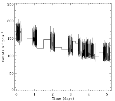
Figure 1.— Light curve in the 2 - 60 keV band from XTE J1751-305 used in our pulsation search. These data span the brightest portion of the outburst onset. Time zero is 2002 Apr 05 at 15:29:03.422 UTC. Note that the background level of $\approx 15$ counts s^-1 PCU^-1 has not been subtracted.

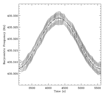
Figure 2.— Dynamic power spectrum (Leahy-normalized) of XTE J1751-305 as a function of time and barycentric frequency in a single RXTE orbit. The contours show levels of Leahy-normalized Fourier power and track the binary Doppler-shifted pulsar spin frequency. The solid curve is the best-fitting orbit model for this data interval. The origin for the time axis has the same reference as Figure 1.

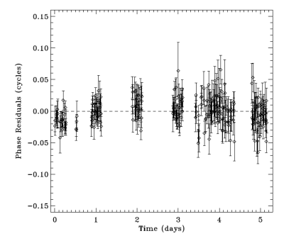
Figure 3.— Pulse timing phase residuals (in cycles) for XTE J1751-305 after application of the best fitting circular orbit model. The remaining phase residuals are poisson dominated. Time zero is the same as in Figure 1.

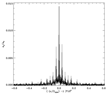
Figure 4.— A portion of the full frequency resolution, coherent power spectrum for XTE J1751-305 in the vicinity of the pulsar spin frequency (at 0 in these units). The power spectrum is shown in units of Fourier amplitudes (see the text in §2 for further details). The side-lobe pattern of peaks results from the uneven temporal sampling (the window function).

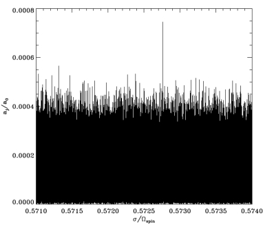
Figure 5.— A portion of the full frequency resolution, coherent power spectrum for XTE J1751-305 in the vicinity of the candidate signal peak at $0.57276\times\nu_{spin}$. The spectrum is plotted in units of fractional Fourier amplitude.

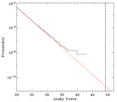
Figure 6.— Probability to exceed a given Leahy-normalized Fourier power in a single trial. The red squares show the expected noise-power distribution (in this case a $\chi^{2}$ distribution with 2 degrees of freedom). The solid histogram shows the observed power-spectral distribution for XTE J1751-305 in the frequency range from 1.6 to 2.2 $\times$ the pulsar spin frequency. The vertical dashed line marks the power value of the candidate signal peak. The data track the expected distribution over a broad range of power values. An exact match at the highest power values is not expected simply due to statistical fluctuations.

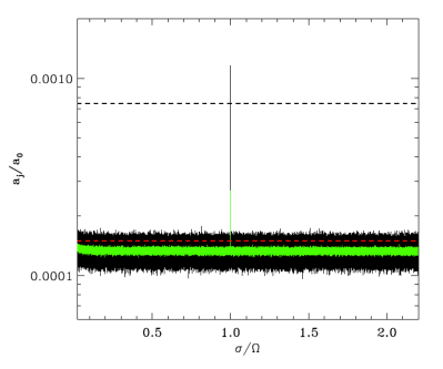
Figure 7.— Frequency-averaged power spectra of XTE J1751-305 plotted in units of fractional Fourier amplitude. Spectra averaged to 1/2048 (black) and 1/128 (green) Hz are shown. The X-axis shows frequency scaled by the pulsar spin frequency. The pulsar signal at 1 is clearly evident, but there are no other significant features evident at either resolution. The horizontal dashed red line marks the amplitude given by $1/\sqrt{N_{tot}}$, where $N_{tot}$ is the total number of counts in the light curve. The horizontal dashed line marks the amplitude of the candidate signal peak at $0.57276\times\nu_{spin}$.

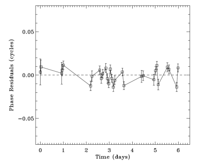
Figure 8.— Pulse timing phase residuals (in cycles) for XTE J1814-338 (first time interval) after application of the best fitting circular orbit model. Time zero is 2003 June 5 at 02:34:20 UTC.

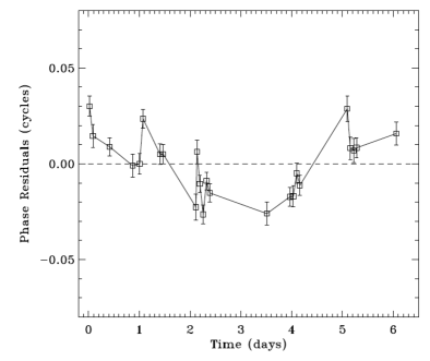
Figure 9.— Pulse timing phase residuals (in cycles) for XTE J1814-338 (second time interval) after application of the best fitting circular orbit model. Time zero is 2003 June 11 at 04:12:28 UTC.

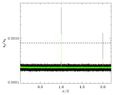
Figure 10.— Frequency-averaged power spectra of XTE J1814-338 (average of both data intervals analyzed) plotted in units of fractional Fourier amplitude. Spectra averaged to 1/2048 (black) and 1/128 (green) Hz are shown. The x-axis shows frequency scaled by the pulsar spin frequency. The pulsar fundamental and first harmonic are clearly evident, but there are no other significant features evident at either resolution. The horizontal dashed red line marks the amplitude given by $1/\sqrt{N_{tot}/2}$, where $N_{tot}$ is the total number of counts in the light curve. The horizontal dashed line (black) marks the upper limit on the amplitude at the full frequency resolution.

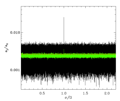
Figure 11.— Frequency-averaged power spectra of NGC 6440 X-2 plotted in units of fractional Fourier amplitude. Spectra at the full frequency resolution (1/3200 Hz, black) and 0.01 Hz (red) are shown. The x-axis shows frequency scaled by the pulsar spin frequency. The pulsar signal at 1 is clearly evident, but there are no other significant features evident at either resolution. The horizontal dashed red line marks the amplitude given by $1/\sqrt{N_{tot}/4}$, where $N_{tot}$ is the total number of counts in the four light curves analyzed.

References

- Aasi et al. (2013) Aasi, J., Abadie, J., Abbott, B. P., et al. 2013, ArXiv e-prints, arXiv:1309.4027
- Alford et al. (2012) Alford, M. G., Mahmoodifar, S., & Schwenzer, K. 2012, Phys. Rev. D, 85, 024007
- Altamirano et al. (2009) Altamirano, D., Strohmayer, T. E., Heinke, C. O., et al. 2009, The Astronomer’s Telegram, 2182, 1
- Altamirano et al. (2010) Altamirano, D., Patruno, A., Heinke, C. O., et al. 2010, ApJ, 712, L58
- Andersson (1998) Andersson, N. 1998, ApJ, 502, 708
- Arras et al. (2003) Arras, P., Flanagan, E. E., Morsink, S. M., et al. 2003, ApJ, 591, 1129
- Bildsten & Cumming (1998) Bildsten, L., & Cumming, A. 1998, ApJ, 506, 842
- Bildsten & Cutler (1995) Bildsten, L., & Cutler, C. 1995, ApJ, 449, 800
- Bildsten et al. (1996) Bildsten, L., Ushomirsky, G., & Cutler, C. 1996, ApJ, 460, 827
- Bondarescu et al. (2007) Bondarescu, R., Teukolsky, S. A., & Wasserman, I. 2007, Phys. Rev. D, 76, 064019
- Carroll et al. (1986) Carroll, B. W., Zweibel, E. G., Hansen, C. J., et al. 1986, ApJ, 305, 767
- Duncan (1998) Duncan, R. C. 1998, ApJ, 498, L45
- Feroci et al. (2012) Feroci, M., den Herder, J. W., Bozzo, E., et al. 2012, in Society of Photo-Optical Instrumentation Engineers (SPIE) Conference Series, Vol. 8443
- Friedman & Morsink (1998) Friedman, J. L., & Morsink, S. M. 1998, ApJ, 502, 714
- Friedman & Schutz (1978) Friedman, J. L., & Schutz, B. F. 1978, ApJ, 222, 281
- Glampedakis & Andersson (2006) Glampedakis, K., & Andersson, N. 2006, Phys. Rev. D, 74, 044040
- Haskell et al. (2012) Haskell, B., Degenaar, N., & Ho, W. C. G. 2012, MNRAS, 424, 93
- Heinke et al. (2010) Heinke, C. O., Altamirano, D., Cohn, H. N., et al. 2010, ApJ, 714, 894
- Heng & Spitkovsky (2009) Heng, K., & Spitkovsky, A. 2009, ApJ, 703, 1819
- Heyl (2005) Heyl, J. S. 2005, MNRAS, 361, 504
- Israel et al. (2005) Israel, G. L., Belloni, T., Stella, L., et al. 2005, ApJ, 628, L53
- Lamb et al. (2009) Lamb, F. K., Boutloukos, S., Van Wassenhove, S., et al. 2009, ApJ, 705, L36
- Lee (2004) Lee, U. 2004, ApJ, 600, 914
- Lee (2010) —. 2010, MNRAS, 405, 1444
- Lee & Strohmayer (2005) Lee, U., & Strohmayer, T. E. 2005, MNRAS, 361, 659
- Levin & Ushomirsky (2001) Levin, Y., & Ushomirsky, G. 2001, MNRAS, 324, 917
- Lindblom et al. (1999) Lindblom, L., Mendell, G., & Owen, B. J. 1999, Phys. Rev. D, 60, 064006
- Lindblom et al. (1998) Lindblom, L., Owen, B. J., & Morsink, S. M. 1998, Physical Review Letters, 80, 4843
- Lockitch & Friedman (1999) Lockitch, K. H., & Friedman, J. L. 1999, ApJ, 521, 764
- Mahmoodifar & Strohmayer (2013) Mahmoodifar, S., & Strohmayer, T. 2013, ApJ, 773, 140
- Markwardt et al. (2003) Markwardt, C. B., Strohmayer, T. E., & Swank, J. H. 2003, The Astronomer’s Telegram, 164, 1
- Markwardt et al. (2002) Markwardt, C. B., Swank, J. H., Strohmayer, T. E., in ’t Zand, J. J. M., & Marshall, F. E. 2002, ApJ, 575, L21
- Markwardt et al. (2007) Markwardt, C. B., Swank, J. H., Strohmayer, T. E., in’t Zand, J. J. M., & Marshall, F. E. 2007, ApJ, 667, L211
- McDermott & Taam (1987) McDermott, P. N., & Taam, R. E. 1987, ApJ, 318, 278
- McDermott et al. (1988) McDermott, P. N., van Horn, H. M., & Hansen, C. J. 1988, ApJ, 325, 725
- Numata & Lee (2010) Numata, K., & Lee, U. 2010, MNRAS, 409, 481
- Owen (2010) Owen, B. J. 2010, Phys. Rev. D, 82, 104002
- Owen et al. (1998) Owen, B. J., Lindblom, L., Cutler, C., et al. 1998, Phys. Rev. D, 58, 084020
- Papitto et al. (2007) Papitto, A., di Salvo, T., Burderi, L., et al. 2007, MNRAS, 375, 971
- Passamonti et al. (2009) Passamonti, A., Haskell, B., Andersson, N., Jones, D. I., & Hawke, I. 2009, MNRAS, 394, 730
- Patruno (2010) Patruno, A. 2010, ApJ, 722, 909
- Patruno & Watts (2012) Patruno, A., & Watts, A. L. 2012, ArXiv e-prints, arXiv:1206.2727
- Patruno et al. (2009) Patruno, A., Wijnands, R., & van der Klis, M. 2009, ApJ, 698, L60
- Piro & Bildsten (2004) Piro, A. L., & Bildsten, L. 2004, ApJ, 603, 252
- Ray et al. (2010) Ray, P. S., Chakrabarty, D., Wilson-Hodge, C. A., et al. 2010, in Society of Photo-Optical Instrumentation Engineers (SPIE) Conference Series, Vol. 7732
- Riggio et al. (2011) Riggio, A., Burderi, L., di Salvo, T., et al. 2011, A&A, 531, A140
- Strohmayer & Bildsten (2006) Strohmayer, T., & Bildsten, L. 2006, New views of thermonuclear bursts, ed. W. H. G. Lewin & M. van der Klis, 113–156
- Strohmayer et al. (1991) Strohmayer, T., van Horn, H. M., Ogata, S., Iyetomi, H., & Ichimaru, S. 1991, ApJ, 375, 679
- Strohmayer & Lee (1996) Strohmayer, T. E., & Lee, U. 1996, ApJ, 467, 773
- Strohmayer et al. (2003) Strohmayer, T. E., Markwardt, C. B., Swank, J. H., & in’t Zand, J. 2003, ApJ, 596, L67
- Strohmayer & Watts (2005) Strohmayer, T. E., & Watts, A. L. 2005, ApJ, 632, L111
- Strohmayer & Watts (2006) —. 2006, ApJ, 653, 593
- Watts (2012) Watts, A. L. 2012, ARA&A, 50, 609
- Watts et al. (2008a) Watts, A. L., Krishnan, B., Bildsten, L., & Schutz, B. F. 2008a, MNRAS, 389, 839
- Watts et al. (2008b) Watts, A. L., Patruno, A., & van der Klis, M. 2008b, ApJ, 688, L37
- Watts & Strohmayer (2006) Watts, A. L., & Strohmayer, T. E. 2006, ApJ, 637, L117
- Woods & Thompson (2006) Woods, P. M., & Thompson, C. 2006, Soft gamma repeaters and anomalous X-ray pulsars: magnetar candidates, ed. W. H. G. Lewin & M. van der Klis, 547–586
- Yoshida & Lee (2000a) Yoshida, S., & Lee, U. 2000a, ApJ, 529, 997
- Yoshida & Lee (2000b) —. 2000b, ApJS, 129, 353
- Yoshida & Lee (2001) —. 2001, ApJ, 546, 1121