Explore or exploit? A generic model and an exactly solvable case

Abstract

Finding a good compromise between the exploitation of known resources and the exploration of unknown, but potentially more profitable choices, is a general problem, which arises in many different scientific disciplines. We propose a stylized model for these exploration-exploitation situations, including population or economic growth, portfolio optimisation, evolutionary dynamics, or the problem of optimal pinning of vortices or dislocations in disordered materials. We find the exact growth rate of this model for tree-like geometries and prove the existence of an optimal migration rate in this case. Numerical simulations in the one-dimensional case confirm the generic existence of an optimum.

The exploration-exploitation tradeoff problem pervades a large number of different fields (see Gen and the many references therein). Two early examples concern the management of firms Exp1 (should one exploit an already known technology or explore other avenues, potentially more profitable, but risky?) and the so-called multi-arm bandit problem Exp3 (sticking with the seemingly most profitable arm to date, or switching in search of potentially more profitable ones?). Clearly, this is a universal paradigm that ranges from population growth and animal foraging to economic growth, investment strategies or optimal research policies. As we will show below, the same issues also arise, in a slightly disguised form, in the context of vortex or dislocation pinning by impurities, and are relevant for material design. Intuitively, neither staying at the same place (and missing interesting opportunities) nor changing places too rapidly (and failing to exploit favorable circumstances) are optimal strategies. An optimal, non zero search rate should thus exist in general. However, there are no exactly solvable cases where the exploration-exploitation tradeoff can be investigated in details. The aim of this paper is to propose a general, stylized model for these exploration-exploitation situations, which encompasses all the examples given above. We obtain exact solutions of this model in two cases (a fully connected and a tree geometry), for which we explicitely prove the existence of a non-trivial optimal search rate. Euclidean geometries are also considered, as these correspond to physical situations, like the pinning problem alluded to above. In this case, perturbation theory and numerical simulations confirm the existence of an optimum as well.

Our model describes the dynamics of a quantity we generically call $Z_{i}$, defined on the nodes $i$ of an arbitrary graph, that evolves according to the following equationBM :

$$\frac{\partial Z_{i}(t)}{\partial t}=\sum_{j\neq i}J_{ij}Z_{j}(t)-\sum_{j\neq i}J_{ji}Z_{i}(t)+\eta_{i}(t)Z_{i}(t).$$ (1)

The first two terms encode “migration” effects, with $J_{ij}$ the migration rate from $j$ to $i$. The last term describes the growth (or decay) of the quantity $Z_{i}$ with a random growth rate $\eta_{i}(t)$. We will choose $\eta_{i}$ to be Gaussian, centred and uncorrelated from site to site, with a exponential time-correlator:

$$\langle\eta_{i}(t_{1})\eta_{j}(t_{2})\rangle=\delta_{ij}\frac{\sigma^{2}}{2\tau}e^{-\frac{|t_{1}-t_{2}|}{\tau}}.$$ (2)

Our qualitative conclusions are however independent of the precise form (2), provided correlations decay on a finite scale $\tau$, which will play an important role in the following.

Many different problems are described by Eq. (1). Population dynamics (bacteria, humans, animals) is one example with $Z_{i}$ the number of individuals around site (or habitat) $i$. In this setting, $\eta_{i}(t)$ encodes the local balance between beneficial and detrimental effects on population growth Nelson (i.e. quality and quantity of resources/nutrients, climate, illnesses, etc.). A slightly different interpretation can be given in the context of evolutionary dynamics, where the sites $i$ correspond to different alleles and the $J_{ij}$ are mutation rates. In the context of pinning problems, $Z_{i}$ corresponds to the partition function of a linear object of length $t$ (polymers, vortices, dislocations), ending on site $i$, that can hop between sites and interact with a local random pinning potential $\eta_{i}(t)$ HHZ . In an economics setting, Eq.(1) can be interpreted as describing the dynamics of the wealth of individuals that exchange and invest in risky projects, or of the total activity in a sector of the economy $i$, that may shift from one sector to another, and grow or decay depending on innovations, raw material prices, etc. Another interesting application is that of portfolio theory, where $Z_{i}$ is the amount of money invested in asset $i$ Cover . Then $\eta_{i}(t)$ is the return streams of this assets and the $J_{ij}$ describe the reallocation of the gains made on some assets towards the rest of the portfolio. Without this rebalancing the portfolio would end up being concentrated in one (or a few) assets only (see e.g. BP , pp. 37-38), and hence be exceedingly risky.

In the case where $J_{ij}\equiv J$ and the nodes $i$ are on a regular lattice in $d$ dimensions, Eq. (1) is a discretized version of the “stochastic heat equation”,

$$\frac{\partial Z(\vec{x},t)}{\partial t}=J\nabla^{2}Z(\vec{x},t)+\eta(\vec{x},t)Z(\vec{x},t).$$ (3)

Upon a Cole-Hopf transformation $Z=e^{h}$, this equation maps into the celebrated KPZ equation $\partial_{t}h=J\nabla^{2}h+J(\nabla h)^{2}+\eta$ that appears in a wide variety of domains: cosmology & turbulence Bec ; BecKhanin , surface growth Krug ; Barabasi , directed polymers HHZ or Hamilton-Jacobi-Bellmann optimisation problems Kappen .

A host of exact results have recently been obtained for the one dimensional ($d=1$) case, in particular concerning the scaling properties of the fluctuations of the $h$-field (for a review, see Corwin ). Here, however, we will not be concerned with these fluctuations but interested in the long-time average “velocity” $c$ of the $h$-field, defined in the discrete case as:

$$c:=\lim_{t\to\infty}\frac{1}{Nt}\sum_{i=1}^{N}\ln Z_{i}(t),$$ (4)

where $N$ is the total number of sites. This velocity $c$ has a clear interpretation in all the examples mentioned above: it represents the average asymptotic growth rate of the population, or of the economic wealth in models of growth, the free-energy of the polymer, vortex, etc. in the context of pinning. It is therefore very natural to look for the maximum of this quantity as a function of the parameters of the model, since these will correspond to optimal situation – either in terms of population, economic or portfolio growth, or in terms of pinning efficiency, which is relevant for material design, for example superconductors with high critical currents HTC . In this case, so-called “columnar disorder” KrugHH (corresponding to a time correlated random noise $\eta$ in the present language) is known to be highly effective at pinning vortices PLD-Nelson ; GiamarchiLedoussal . Our central result is that for non-zero correlation time of the random noise/potential $\eta_{i}(t)$, there exists an optimal migration rate $J$ such that $c$ reaches a maximum. This optimal rate realizes the “exploration-exploitation” compromise: moving too slowly ($J$ small) does not allow the system to probe the environment efficiently, and some favorable opportunities are missed. Moving too fast ($J$ large), on the other hand, does not allow the system to fully benefit from favorable spots that last for a time $\sim\tau$, as it leaves these spots too early.

Let us first present numerical simulations of the 1+1 directed polymer problem with time-correlated disorder. The equation we simulated is:

$$Z_{i}(t+\mathrm{d}t) =(1-2J\mathrm{d}t)Z_{i}(t)+$$

$$J\mathrm{d}t \left[Z_{i+1}(t)+Z_{i-1}(t)\right]+\eta_{i}(t)\mathrm{d}tZ_{i}(t),$$ (5)

with $i=1,\dots,N$ and $\eta_{i}(t)$ an exponentially correlated Gaussian noise, as in Eq. (2). We considered a system with $N=512$ sites and periodic boundary conditions. We determined $c(J)$ after a time $t=40$ long enough to reach a stationary state, and much greater than the correlation time fixed here to $\tau=0.1$. The dependence of $c$ on $J$ for $\sigma=1$ and $\tau=0.1$ is shown in Fig. 1, together with a) the result of direct perturbation theory of the KPZ equation, a priori valid for large $J$, and b) the prediction of the “tree-approximation” with $a=1/2$ and $m=1$ that we detail below. The former predicts $c(J)\approx\sigma^{2}/4\sqrt{J\tau}+O(\sigma^{4}/J)$ for $J\to\infty$, which indeed fits the data quite well in the large $J$ region, without any adjustable parameter. The tree-approximation, on the other hand, is quantitatively incorrect as expected for a one-dimensional system. For example, it predicts a $J^{-1}$ decay of $c$ (see below) but still manages to capture approximately the overall behaviour of $c(J)$, in particular the existence of a maximum.

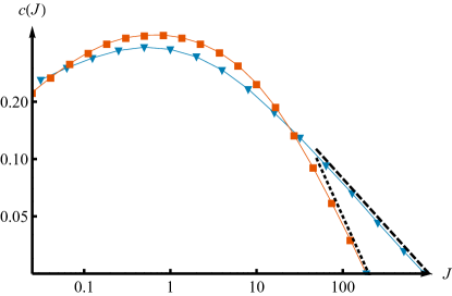
Figure 1: Comparison of simulations of (5) (blue triangles) and of (6) (red squares) for $N=512$ and $\tau=0.1$, as functions of the branching (diffusion) rate $J$. We fix $\sigma=1$. The dashed black line is the large $J$ asymptotics obtained from perturbation theory, $c(J)\approx\sigma^{2}/4\sqrt{J\tau}$. The dotted line reveals the $J^{-1}$ behaviour of $c(J)$ for large $J$, predicted by the tree-approximation (with $a=1/2$ and $m=1$).

Let us now turn to a simplified model, where the interplay between exploration and exploitation, and the optimal migration rate, can be fully understood analytically. We first note that our general model Eq. (1) for a regular lattice with $J_{ij}=J$ for neighbouring sites, can be slightly altered as the following evolution rule:

$$Z_{i}(t+\mathrm{d}t)=\begin{cases}Z_{i}(t+\mathrm{d}t)\exp\left[\eta_{i}(t)\mathrm{d}t\right]&\text{prob.}\,1-J\mathrm{d}t,\\ (1-{a})Z_{i}(t)+\frac{a}{m}\sum_{j\wedge i}Z_{j}(t)&\text{prob.}\,J\mathrm{d}t.\end{cases}$$ (6)

where $m$ is the number of neighbours of $i$ and $j\wedge i$ means that $i,j$ are neighbours. To obtain a solvable model, we neglect all spatial correlations between the $Z_{i}$’s, which amounts to the tree approximation introduced by Derrida and Spohn for the directed polymer problem in 1988 DerridaSpohn1988 . Following these authors, we define the generating functions

$$G_{t}(x,\eta):= \left\langle\exp\left[-e^{-x}Z_{i}(t)\right]\delta\left[\eta_{i}(t)-\eta\right]\right\rangle,$$

$$\widehat{G}_{t}(x):= \int_{-\infty}^{\infty}\mathrm{d}\eta\,G_{t}(x,\eta)=\left\langle\exp\left[-e^{-x}Z_{i}(t)\right]\right\rangle$$ (7)

Assuming the $Z_{i}$’s to be independent allows one to write the following evolution equation for $G_{t}(x,\eta)$:

$$G_{t+\mathrm{d}t}(x,\eta)=$$

$$(1-J\,\mathrm{d}t)\langle\exp\left[-e^{-x+\eta_{i}(t)\mathrm{d}t}Z_{i}(t)\right]\delta\left[\eta_{i}(t+\mathrm{d}t)-\eta\right]\rangle$$

$$+J\,\mathrm{d}t\left\langle\exp\left[-e^{-x+q_{1}}Z_{i}(t)\right]\delta\left[\eta_{i}(t)-\eta\right]\right\rangle$$

$$\times\left\langle\exp\left[-e^{-x+q_{2}}Z_{j}(t)\right]\right\rangle^{m}$$ (8)

with $q_{1}:=\log(1-{a})$ and $q_{2}:=\log\frac{a}{m}$. The choice in Eq. (2) of an Ornstein-Uhlenbeck process for $\eta$ is particularly simple, since it yields a Markovian equation for $\eta_{i}(t+\mathrm{d}t)$:

$$\eta_{i}(t+\mathrm{d}t)=\eta_{i}(t)+\left[-\frac{1}{\tau_{c}}\eta_{i}(t)+\frac{\sigma}{\tau_{c}}\xi_{i}(t)\right]\mathrm{d}t,$$ (9)

where $\xi$ is a Gaussian white noise. Inserting this into (Explore or exploit? A generic model and an exactly solvable case), and expanding to $\mathcal{O}(\mathrm{d}t)$, we obtain

$$G_{t+\mathrm{d}t}(x,\eta)= \left\langle G_{t}\left(x,\eta+\frac{\sigma}{\tau_{c}}\xi_{i}(t)\mathrm{d}t\right)\right\rangle_{\xi}-J\,\mathrm{d}tG_{t}(x,\eta)$$

$$-\eta\,\mathrm{d}t\,\partial_{x}G_{t}(x,\eta)+\frac{\mathrm{d}t}{\tau}\partial_{\eta}\left[\eta G_{t}(x,\eta)\right]$$

$$+J\,\mathrm{d}t\,G_{t}(x-q_{1},\eta)\widehat{G}_{t}(x-q_{2})^{m}+\mathcal{O}(\mathrm{d}t)^{2}$$

Using $\xi_{i}(t)\mathrm{d}t\sim\mathcal{N}(0,\mathrm{d}t)$, we now average over $\xi$ and obtain a generalized Fisher-KPP equation for $G$, where the diffusion operator is replaced by the Ornstein-Uhlenbeck operator, involving the additional state variable $\eta$:

$$\partial_{t}G_{t}(x,\eta)= \frac{\sigma^{2}}{2\tau_{c}^{2}}\partial_{\eta}^{2}G+\frac{1}{\tau_{c}}\partial_{\eta}\left(\eta G\right)-\eta\partial_{x}G$$

$$+J\left[G_{t}(x-q_{1},\eta)\widehat{G}_{t}(x-q_{2})^{m}-G_{t}(x,\eta)\right].$$ (10)

Like the Fisher-KPP equation known from the standard mean-field directed polymer problem DerridaSpohn1988 ; CookDerrida1990 , it gives rise to a front propagating in the $x$ direction. The velocity of this front is precisely the quantity $c$ we are looking for and is fixed by the tail behaviour of $G_{t}$ when $x\to\infty$. In this tail, we make the following ansatz for $G$:

$$G_{t}(x,\eta)=Q(\eta)-R(\eta)e^{-\gamma(x-ct)}+...$$ (11)

with $\int\mathrm{d}\eta\,Q(\eta)=1$. Inserting this into (10), one finds, by identifying terms of order $1$ and terms of order $e^{-\gamma(x-ct)}$, that $Q(\eta)$ is the stationary Gaussian distribution for the Ornstein-Uhlenbeck process $\eta(t)$ (as it should be), while $R(\eta)$ satisfies:

$$Rc\gamma= \frac{\sigma^{2}}{2\tau^{2}}\partial^{2}_{\eta}R+\frac{1}{\tau}\partial_{\eta}(\eta R)+\eta R+Jme^{\gamma q_{2}}Q\int\mathrm{d}\eta R(\eta)$$

$$+R(\eta)J(e^{\gamma q_{1}}-1).$$ (12)

This can be simplified by imposing (without loss of generality) $\int\mathrm{d}\eta\,R(\eta)=1$ and setting $R=\phi e^{-\eta^{2}\tau/2\sigma^{2}}$, $\sigma^{2}\hat{c}=\gamma c-J(e^{\gamma q_{1}}-1)-\sigma^{2}\gamma^{2}/2$ and $y=\eta/\sigma^{2}-\gamma$. One gets the following equation for $\phi$:

$$-\frac{1}{2\sigma^{4}\tau^{2}}\phi^{\prime\prime}+\frac{1}{2}y^{2}\phi+(\hat{c}-\frac{1}{2\sigma^{2}\tau})\phi=\frac{Jme^{\gamma q_{2}}}{\sigma^{2}}\frac{e^{-\frac{(y+1)^{2}\sigma^{2}\tau}{2}}}{\sqrt{\pi\sigma^{2}/\tau}}.$$ (13)

Introducing the harmonic oscillator eigenfunctions $\phi_{n}(y)=e^{-y^{2}\sigma^{2}\tau/2}H_{n}(y\sigma\sqrt{\tau})$, the solution of the above equation can be written as $\phi(y)=\sum_{n=0}^{\infty}A_{n}\phi_{n}(y)$ where the coefficients $A_{n}$ are given by:

$$A_{n}\left[\frac{n}{\sigma^{2}\tau}+\hat{c}\right]=\frac{Jme^{\gamma q_{2}}}{\sigma^{2}}\frac{e^{-\gamma^{2}\sigma^{2}\tau/4}\frac{(-1)^{n}}{n!}\left(\frac{\sigma\sqrt{\tau}}{2}\right)^{n}}{\sqrt{\pi\sigma^{2}/\tau}}.$$ (14)

Finally, the condition $\int\mathrm{d}\eta\,R(\eta)=1$ yields an implicit equation for $c$, valid for arbitrary $\tau$ :

$$1=Jme^{\gamma q_{2}-\gamma^{2}\sigma^{2}\tau/2}\sum_{n=0}^{\infty}\frac{(\gamma^{2}\sigma^{2}\tau/2)^{n}}{n!\left[\frac{n}{\tau}+\gamma c-J(e^{\gamma q_{1}}-1)-\frac{\sigma^{2}}{2}\gamma^{2}\right]}$$ (15)

As in the Derrida-Spohn case, the corresponding function $c(\gamma)$ is found to reach a minimum value for a certain $\gamma_{\min}$, that depends on the parameters $J,\sigma^{2},\tau,m$. The interpretation of this phenomenon is now standard: only traveling waves with $\gamma\leq\gamma_{\min}$ can be sustained, and propagate at the speed $c(\gamma)$. A wave front which is “too sharp”, i.e. prepared initially with a $\gamma>\gamma_{\min}$, will broaden until it reaches $\gamma=\gamma_{\min}$, and will propagate with the velocity $c(\gamma_{\min})$. In our case, the initial condition $Z=1$ corresponds to $\gamma=1$; therefore either $\gamma_{\min}$ is found to be larger than unity, in which case $c$ is given by the solution of Eq. (15) with $\gamma=1$, or $\gamma_{\min}\leq 1$, in which case $c=c(\gamma_{\min})$. For the directed polymer/pinning problem, the first case corresponds to the high-temperature, annealed phase (arising for $J\geq J_{c}$), while the second case corresponds to a low-temperature, frozen phase (for $J\leq J_{c}$). In the random growth problems, the latter case corresponds to a localization of the population/wealth/portfolio on a small number of particularly favorable habitats/individuals/assets (see the discussion in BM ).

We determine $c(\gamma)$, $\gamma_{\min}$ and $c(\gamma_{\min})$ numerically from (15), with very good agreement with numerical simulations (see figure 2). We see in particular that for $\tau=0$, increasing the migration rate always increases the growth rate, which saturates at a constant value $c=\sigma^{2}/2$, for all $J\geq J_{c}$. Therefore, no optimum tradeoff between exploration and exploitation exists in this case – exploring is always favorable or neutral. However, when a finite correlation time $\tau$ is introduced, we see that, as expected, an optimum migration rate indeed appears (cf. figure 2). In particular, we find analytically that for small $J$, $c(J)=\sqrt{2\sigma^{2}J}+\mathcal{O}(J)$ while for large $J$, $c(J)=\sigma^{2}/{2aJ\tau}+\mathcal{O}(J)^{-2}$. In fact, the large $J$ behaviour can be understood heuristically as follows. Clearly, the problem for $\tau>0$ must be equivalent, for large times, to the standard uncorrelated case ($\tau=0$), but with a renormalized disorder amplitude. For large $J$ and finite $\tau$, the disorder cannot change the random walk nature of the exploration up to time $\tau$. The walk therefore freely visits $N_{\neq}=\mathcal{O}(J\tau)$ different sites during this time, leading to a pre-averaging of the random disorder that reduces the variance $\sigma^{2}$ by a factor $N_{\neq}$. Since for $\tau=0$, $c\propto\sigma^{2}$, the above renormalisation immediately leads to $c(J)\sim\sigma^{2}/{J\tau}$ at large $J$. [Note that the very same argument leads to $c(J)\sim\sigma^{2}/\sqrt{J\tau}$ in $d=1$, as found above, and is also exact in $d=2$, where logarithmic corrections appear.] Now since $c(J=0)=0$ trivially, the decaying behaviour of $c(J)$ for large $J$ and finite $\tau$ immediately implies the generic existence of an optimum in the exploration rate, as anticipated above.

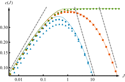
Figure 2: (Color online) Comparison of simulations of (6) for various $N$ and $\tau$, as a function of the branching (diffusion) rate $J$. Green diamonds, orange squares and blue circles were obtained from numerical simulation of (6) for $\tau=0,0.1$ and $1$ with $N=2^{20}$. Blue triangles correspond to $\tau=1$ and $N=2^{8}$. In all cases, $\sigma=1$ and $a=1/2$, $m=1$. The solid curves were obtained by numerical solution of (15) for the corresponding values of $\tau$. The dashed grey lines are the large and small-$J$ asymptotics.

We find very similar conclusions isunpublished for another exactly solvable limit, the fully connected graph where $J_{ij}=J_{0}/N$, $\forall i,j$, which in fact corresponds (up to minor details) to the limit $a=1-\frac{1}{N}$ and $m=N$ of the tree model above. Other theoretical methods used to investigate the KPZ/Directed Polymer problem could also be useful to characterize $c(J)$ in $d+1$ dimensions or for other geometries, such as Mode-Coupling Theory or the Gaussian Variational method. The mapping to interacting bosons in the 1+1 case is also an interesting avenue we are exploring isunpublished . It would be very interesting to observe the predicted pinning optimum experimentally. One possibility is in superconductors where the hopping rate $J$ is related to the elastic energy of the vortex lattice, which itself depends on the external magnetic field. Changing the temperature is also a way to affect both the hopping constant and the effective pinning strength RossoPLD . Applications of these ideas are numerous, in particular to quantify how diversified portfolios benefit from a balance between persistence and rebalancing, or to understand how economic growth is impacted by the ability of societies to find a tradeoff between tradition and innovation, or else collapse collapse .

We thank G. Biroli, P. Le Doussal and R. Munos for very helpful insights.

References

- [1] J. D. Cohen, S. M. McClure, and A. J. Yu. Philos Trans R Soc Lond B Biol Sci, 362(1481):933–942, 2007.
- [2] J. G. March. Exploration and exploitation in organizational learning. Organization Science, 2(1):71–87, 1991. Note that it has 11,000 citations at the time of writing !
- [3] J. C. Gittins and D. M. Jones. A dynamic allocation index for the sequential design of experiments. In Progress in statistics (European Meeting Statisticians, Budapest, 1972), pages 241–266. North-Holland, Amsterdam, 1974.
- [4] J.P. Bouchaud and M. Mézard. Wealth condensation in a simple model of economy. Physica A, 282(3–4):536–545, 2000.
- [5] D. R. Nelson and N. M. Shnerb. Non-hermitian localization and population biology. Phys. Rev. E, 58(2):1383–1403, 1998.
- [6] T. Halpin-Healy and Y.-C. Zhang. Kinetic roughening phenomena, stochastic growth, directed polymers and all that. aspects of multidisciplinary statistical mechanics. Physics Reports, 254(4–6):215–414, 1995.
- [7] T. M. Cover. Universal portfolios. Mathematical Finance, 1:1–29, 1991.
- [8] J.-P. Bouchaud and M. Potters. Theory of Financial Risks and Derivative Pricing. Cambridge University Press, 2003.
- [9] U. Frisch and J. Bec. Burgulence. In M. Lesieur, A. Yaglom, and F. David, editors, New trends in turbulence Turbulence: nouveaux aspects, pages 341–383. Springer Berlin Heidelberg, 2001.
- [10] J. Bec and K. Khanin. Burgers turbulence. Physics Reports, 447(1–2):1 – 66, 2007.
- [11] J. Krug and H. Spohn. Kinetic roughening of growing surfaces in Solids Far from Equilibrium. C. Godrèche, Cambridge University Press, 1991.
- [12] A.-L. Barabasi and H. E. Stanley. Fractal Concepts in Surface Growth. Cambridge University Press, 1995.
- [13] H. J. Kappen. Linear theory for control of nonlinear stochastic systems. Phys. Rev. Lett., 95(20):200–201, 2005.
- [14] I. Corwin. The Kardar-Parisi-Zhang equation and universality class. Random Matrices: Theory and Applications, 01(01):1130001, 2012.
- [15] B. Maiorov and al. Synergetic combination of different types of defect to optimize pinning landscape using BaZrO3-doped YBa2Cu3O7. Nat Mater, 8(5):398–404, 2009.
- [16] J. Krug and T. Halpin-Healy. Directed polymers in the presence of columnar disorder. J. Phys. I France, 3(11), 1993.
- [17] T. Hwa, P. Le Doussal, D. Nelson, and V. Vinokur. Flux pinning and forced vortex entanglement by splayed columnar defects. Phys. Rev. Lett., 71(21):3545–3548, 1993.
- [18] T. Giamarchi and P. Le Doussal. Variational theory of elastic manifolds with correlated disorder and localization of interacting quantum particles. Phys. Rev. B, 53:15206–15225, 1996.
- [19] B. Derrida and H. Spohn. Polymers on disordered trees, spin glasses, and traveling waves. J Stat Phys, 51(5-6):817–840, 1988.
- [20] J. Cook and B. Derrida. Polymers on disordered hierarchical lattices: A nonlinear combination of random variables. Journal of Statistical Physics, 57(1-2):89–139, 1989.
- [21] The infinite sum over can be rewritten in a integral form that is convenient for an asymptotic analysis of the equation.
- [22] Note that the “columnar” limit where [16, 17, 18], is not easily approachable through the KPP mapping due to the non commutativity of the large and large limits.
- [23] T. Gueudré, A. Dobrinevski, and J-P. Bouchaud. in preparation.
- [24] S. Bustingorry, P. Le Doussal, and A. Rosso. Universal high-temperature regime of pinned elastic objects. Phys. Rev. B, 82(14):140201, 2010.
- [25] J. M. Diamond. Collapse: How Societies Choose to Fail Or Succeed. Penguin, 2006.