On the stabilization of the Friedmann Big Bang by the shear stresses

Abstract

The window is found in the space of the free parameters of the theory of viscoelastic matter for which the Friedmann singularity is stable. Under stability we mean that in the presence of the shear stresses the generic solution of the equations of relativistic gravity possessing the isotropic, homogeneous and thermally equilibrated cosmological singularity exists.

I Introduction

Observations show that the early Universe was isotropic, homogeneous and thermally balanced. A number of authors Bar ; Pen ; Goo expressed the point of view that also the initial cosmological singularity should be in conformity with these properties, that is should be of the Friedmann type. But it is well known that the Friedmann singularity for the conventional types of matter is unstable which means that space-time cannot start isotropic expansion unless an artificial fine tuning of unknown origin. This instability is due to the sharp anisotropy which develops unavoidably near the generic cosmological singularity. However, an intuitive understanding suggests that anisotropy can be damped down by the shear viscosity which being taking into account might results in the generic solution with isotropic Big Bang. To search an analytical realization of such a possibility there would be inappropriate to use just the Eckart Eck or Landau-Lifschitz LL approaches to the relativistic hydrodynamics with dissipative processes. These theories are valid provided the characteristic times of the macroscopic motions of the matter are much bigger than the time of relaxation of the medium to the equilibrium state. It might happen that this is not so near the cosmological singularity since all characteristic macroscopic times in this region tend to zero in which case one need a theory which takes into account the Maxwell’s relaxation times on the same footing as all other transport coefficients. In a literal sense such a theory does not exists, however, it can be constructed in an approximate form for the cases when a medium do not deviates too much from equilibrium and relaxation times do not exceed noticeably the characteristic macroscopic times . It is reasonable to expect that these conditions will be satisfied automatically for a generic solution (if it exists) near isotropic singularity describing the beginning of the thermally balanced Friedmann Universe accompanying by the arbitrary infinitesimally small corrections.

The main target of the efforts of many authors (starting from the first idea of Cattaneo Cat up to the final formulation of the generalized relativistic theory by Israel and Stewart Isr1 ; Isr2 ) was to bring the theory into line with relativistic causality, that is to eliminate the supraluminal propagation of the thermal and viscous excitations. The existence of such supraluminal effects was the main stumbling-block for the Eckart’s and Landau-Lifschitz’s descriptions of dissipative fluids. One of the first applications of the Israel-Stewart theory to the problems of cosmological singularity was undertaken in the article BNK . Already in this paper the stability of the Friedmann models under the influence of the shear viscosity has been investigated and it was found that relativistic causality and stability of the Friedmann singularity are in contradiction to each other. Then the final conclusion was: ”…relativistic causality precludes the stability of isotropic collapse. The isotropic singularity cannot be the typical initial or final state.” However, in the present paper it will be shown that this ”no go” conclusion was too hasty since it was the result of too restricted range for the dependence of the shear viscosity coefficient on the energy density. As usual, in the vicinity to the singularity where the energy density $\varepsilon$ diverges we approximate the coefficient of viscosity $\eta$ by the power law asymptotics $\eta\sim\varepsilon^{\nu}$ with some exponent $\nu.$ In the article BNK (due to some more or less plausible thoughts) we choose the values of this exponent from the region $\nu>1/2.$ For these values of $\nu$ the negative result of paper BNK remains correct, but recently it made known that the boundary value $\nu=1/2$ leads to the dramatic change of the state of affairs. It turns out that for this case there exists a window in the space of the free parameters of the theory in which the Friedmann singularity becomes stable and at the same time no supraluminal signals exist in its vicinity. This possibility was overlooked in BNK .

It is worth to add that also the case $\nu<1/2$ is analyzed in the present article but it is of no interest since it leads to the strong instability of the isotropic singularity independently of the question of relativistic causality.

Also it is necessary to stress that here as well as in the old paper BNK only the standard models for a physical fluid is considered for which the pressure is non-negative and is less than the energy density.

To make the present paper self-contained we will reproduce below the principal (although updated) points on which the analysis of the work BNK was based. Then to read the present paper there is no necessity to turn to our old publication.

II Basic equations in the presence of the shear stresses

Shear stresses generate an addend $S_{ik}$ to the standard energy-momentum tensor of a fluid:

$$T_{ik}=\left(\varepsilon+p\right)u_{i}u_{k}+pg_{ik}+S_{ik}\text{ },$$ (1)

and this additional term has to satisfy the following constraints LL :

$$S_{ik}=S_{ki}\text{ },\text{ }S_{k}^{k}=0\text{ },\text{ }u^{i}S_{ik}=0\text{ }.$$ (2)

Besides we have the usual normalization condition for the 4-velocity:

$$u_{i}u^{i}=-1.$$ (3)

If the Maxwell’s relaxation time $\tau$ of the stresses is not zero then do not exists any closed expression for $S_{ik}$ in terms of the viscosity coefficient $\eta$ and 4-gradients of the 4-velocity. Instead the stresses $S_{ik}$ should be defined from the following differential equations Isr1 :

$$S_{ik}+\tau\left(\delta_{i}^{m}+u_{i}u^{m}\right)\left(\delta_{k}^{n}+u_{k}u^{n}\right)S_{mn}{}_{;l}u^{l}=$$ (4)

$$=-\eta\left(u_{i;k}+u_{k;i}+u^{l}u_{k}u_{i;l}+u^{l}u_{i}u_{k;l}\right)+$$

$$+\frac{2}{3}\eta\left(g_{ik}+u_{i}u_{k}\right)u^{l}{}_{;l}\text{ },$$

which due to the normalization condition for velocity is compatible with constraints (2). In case $\tau=0$ expression for $S_{ik},$ following from this equation, coincides with that one introduced by Landau and Lifschitz LL . If the equations of state $p=p\left(\varepsilon\right),$ $\eta=\eta\left(\varepsilon\right),$ $\tau=\tau\left(\varepsilon\right)$ are fixed then the Einstein equations

$$R_{ik}=T_{ik}-\frac{1}{2}g_{ik}T_{l}^{l}$$ (5)

together with equation (4) for the stresses gives the closed system where from all quantities of interest, that is $g_{ik},u_{i},\varepsilon,S_{ik}$ can be found.

Since we are interesting in behaviour of the system in the vicinity to the cosmological singularity where $\varepsilon\rightarrow\infty$ the viscosity coefficient $\eta$ in this asymptotic domain can be approximated by the power law asymptotics

$$\eta=const\cdot\varepsilon^{\nu},$$ (6)

with some constant exponent $\nu.$ Beforehand the value of this exponent is unknown then we need to investigate its entire range $-\infty<\nu<\infty.$ As for the relaxation time $\tau$ the choice is more definite. It is well known that $\eta/\varepsilon\tau$ represents a measure of velocity of propagation of the shear excitations. Then we will model this ratio by a positive constant $f$ (in a more accurate theory $f$ can be a slow varying function on time but in any case this function should be bounded in order to exclude the appearance of the supraluminal signals). Consequently we choose the following model for the relation between relaxation time and viscosity coefficient:

$$\eta=f\varepsilon\tau,\text{ }f=const.$$ (7)

For the dependence $p=p\left(\varepsilon\right)$ we follow the standard approximation with constant parameter $\gamma$:

$$p=\left(\gamma-1\right)\varepsilon\text{ },\text{ }1\leqslant\gamma<2.$$ (8)

Now the system (1)-(8) is closed and we can search the asymptotic behaviour of its solution in the vicinity to the cosmological singularity. It is convenient to work in the synchronous reference system where the interval is

$$-ds^{2}=-dt^{2}+g_{\alpha\beta}dx^{\alpha}dx^{\beta}.$$ (9)

Our task is to take the standard Friedmann solution in this system as background and to find the asymptotic (near singularity) solution of the equations (1)-(8) for the linear perturbations around this background in the same synchronous system. The background solution is:

$$-ds^{2} =-dt^{2}+R^{2}\left[\left(dx^{1}\right)^{2}+\left(dx^{2}\right)^{2}+\left(dx^{3}\right)^{2}\right],\text{ }$$ (10)

$$R =\left(t/t_{c}\right)^{2/3\gamma},\text{ }$$

$$\varepsilon=4\left(3\gamma^{2}t^{2}\right)^{-1},\text{ }u_{0}=-1,\text{ }u_{\alpha}=0,\text{ }S_{ik}=0,$$ (11)

where $t>0$ and $t_{c}$ is some arbitrary positive constant (it is worth to remark that in the comoving and at the same time synchronous system the right hand side of the equation (4) is identically zero then the background value $S_{ik}=0$ indeed satisfies this equation). We have to deal with the following linear perturbations (as usual any quantity $X$ we write as $X=X_{\left(0\right)}+\delta X$ where $X_{\left(0\right)}$ represents the background value of $X$ ):

$$\delta g_{\alpha\beta},\delta u_{\alpha},\delta\varepsilon,\delta S_{\alpha\beta}.$$ (12)

In the linearized version of the system (1)-(9) around the Friedmann solution (10)-(11) will appear only these variations. The variations $\delta u_{0}$ and $\delta S_{0k}$ can not be of the first (linear) order because of the exact relations $u_{i}u^{i}=-1$ and $u^{i}S_{ik}=0$ and properties (11) of the background. The variations $\delta\tau$ and $\delta\eta$ of the relaxation time and viscosity coefficient, although exist as the first order quantities, will disappear from the linear approximation since they reveal itself only as factors in front of the terms vanishing for the isotropic Friedmann seed.

Let’s introduce for the quantities (12) the following notations:

$$\delta g_{\alpha\beta}=R^{2}H_{\alpha\beta},\text{ }\delta u_{\alpha}=V_{\alpha},\text{ }\delta\varepsilon=E,\text{ }\delta S_{\alpha\beta}=R^{2}K_{\alpha\beta}.$$ (13)

(Here and in the sequel we use two different entries $\delta^{\alpha\beta}$ and $\delta_{\alpha\beta}$ for one and the same 3-dimensional Kronecker delta). In terms of these quantities the linearized version of the equations (1)-(5) in synchronous reference system over the Friedmann space-time (10)-(11) becomes:

$$\ddot{H}_{\alpha\beta}+\frac{3\dot{R}}{R}\dot{H}_{\alpha\beta}+\frac{\dot{R}}{R}\delta_{\alpha\beta}\dot{H}+$$ (14)

$$+\frac{1}{R^{2}}\left(\delta^{\lambda\mu}H_{\alpha\lambda},_{\beta\mu}+\delta^{\lambda\mu}H_{\beta\lambda},_{\alpha\mu}-\delta^{\lambda\mu}H_{\alpha\beta},_{\lambda\mu}-H,_{\alpha\beta}\right)=$$

$$=\left(2-\gamma\right)\delta_{\alpha\beta}E+2K_{\alpha\beta}\text{ },$$

$$\dot{H},_{\alpha}-\delta^{\lambda\mu}\dot{H}_{\alpha\lambda},_{\mu}=2\gamma\varepsilon V_{\alpha}\text{ },$$ (15)

$$\ddot{H}+\frac{2\dot{R}}{R}\dot{H}=\left(2-3\gamma\right)E\text{ },$$ (16)

$$K_{\alpha\beta}+\tau\dot{K}_{\alpha\beta}=-\frac{\eta}{R^{2}}\left(V_{\alpha},_{\beta}+V_{\beta},_{\alpha}\right)+$$ (17)

$$+\frac{2\eta}{3R^{2}}\delta_{\alpha\beta}\delta^{\lambda\mu}V_{\lambda},_{\mu}-\eta\left(\dot{H}_{\alpha\beta}-\frac{1}{3}\delta_{\alpha\beta}\dot{H}\right),$$

where $H=\delta^{\alpha\beta}H_{\alpha\beta}$. In these formulas $R$ is the background scale factor given in (10) and $\varepsilon,\tau,\eta$ are the background values of these quantities defined by the the relations (6), (7) and (11) (in principle they should be written as $\varepsilon_{\left(0\right)},\tau_{\left(0\right)},\eta_{\left(0\right)}$ but we omit the index $\left(0\right)$ to simplify the writing).

To find the general solution of these equations we apply the technique invented by Lifschitz L1 (see also LK ) and used by him to analyze the stability of the Friedmann solution for the perfect liquid. Since all coefficients in the differential equations (14)-(17) do not depend on spatial coordinates we can represent all quantities of interest in the form of the 3-dimensional Fourier integrals to reduce these equations to the system of the ordinary differential equations in time for the corresponding Fourier coefficients. First of all we substitute the expression for $E$ from equation (16) to the right hand side of equation (14) and expression for $V_{\alpha}$ from (15) to the right hand side of (17). This gives the closed system of equations for tensorial perturbations $H_{\alpha\beta}$ and $K_{\alpha\beta}$ and corresponding system of ordinary differential equations in time for their Fourier coefficients $\tilde{H}_{\alpha\beta}$ and $\tilde{K}_{\alpha\beta}$ (any space-time field $\Phi\left(t,x^{1},x^{2},x^{3}\right)$ we represent as $\Phi\left(t,x^{1},x^{2},x^{3}\right)={\displaystyle\int}\tilde{\Phi}\left(t,k_{1},k_{2},k_{3}\right)e^{ik_{\alpha}x^{\alpha}}d^{3}k$). Any symmetric tensorial Fourier coefficient containing six independent components can be expended in the Lifshitz basis which consists of the six basic elements. These elements can be constructed from an orthonormal triad $\left(l_{\alpha}^{\left(1\right)},l_{\alpha}^{\left(2\right)},l_{\alpha}^{\left(3\right)}\right)$ in the euclidean $k$-space where

$$l_{\alpha}^{\left(1\right)}=k_{\alpha}/k\text{ },\text{ }k=\sqrt{\delta^{\alpha\beta}k_{\alpha}k_{\beta}}),$$ (18)

that is $l_{\alpha}^{\left(1\right)}$ is the unit directional vector of $k$-space and $l_{\alpha}^{\left(2\right)},l_{\alpha}^{\left(3\right)}$ are another two unit vectors normal to $k_{\alpha}$ and to each other. The aforementioned basic elements are:

$$Q_{\alpha\beta}=\frac{1}{3}\delta_{\alpha\beta}\text{ },\text{ \ }P_{\alpha\beta}=\frac{1}{3}\delta_{\alpha\beta}-\frac{k_{\alpha}k_{\beta}}{k^{2}},$$ (19)

$$L_{\alpha\beta}^{\left(2\right)}=\frac{k_{\alpha}}{k}l_{\beta}^{\left(2\right)}+\frac{k_{\beta}}{k}l_{\alpha}^{\left(2\right)},\text{ }L_{\alpha\beta}^{\left(3\right)}=\frac{k_{\alpha}}{k}l_{\beta}^{\left(3\right)}+\frac{k_{\beta}}{k}l_{\alpha}^{\left(3\right)},$$ (20)

$$G_{\alpha\beta}^{\left(2\right)}=l_{\alpha}^{\left(2\right)}l_{\beta}^{\left(3\right)}+l_{\beta}^{\left(2\right)}l_{\alpha}^{\left(3\right)},\text{ }G_{\alpha\beta}^{\left(3\right)}=l_{\alpha}^{\left(2\right)}l_{\beta}^{\left(2\right)}-l_{\alpha}^{\left(3\right)}l_{\beta}^{\left(3\right)}.$$ (21)

Then $\tilde{H}_{\alpha\beta}$ and $\tilde{K}_{\alpha\beta}$ can be expended in the following way:

$$\tilde{H}_{\alpha\beta}=\lambda P_{\alpha\beta}\text{ }+\mu Q_{\alpha\beta}+{\displaystyle\sum\limits_{J=2}^{3}}\left[\sigma_{\left(J\right)}L_{\alpha\beta}^{\left(J\right)}+\omega_{\left(J\right)}G_{\alpha\beta}^{\left(J\right)}\right],$$ (22)

$$\tilde{K}_{\alpha\beta}=AP_{\alpha\beta}\text{ }+{\displaystyle\sum\limits_{J=2}^{3}}\left[B_{\left(J\right)}L_{\alpha\beta}^{\left(J\right)}+D_{\left(J\right)}G_{\alpha\beta}^{\left(J\right)}\right],$$ (23)

(here we introduced the new index $J$ which takes only two values $2$ and $3$), where the amplitudes $\lambda,\mu,\sigma_{\left(J\right)},\omega_{\left(J\right)},A,B_{\left(J\right)},D_{\left(J\right)}$ depend on time (and on the components of the wave vector).

Only $Q_{\alpha\beta}$ has non-zero contraction $\delta^{\alpha\beta}Q_{\alpha\beta}$ , that’s why in the expansion (23) for the shear stresses this component is absent (remember that the second condition of (2) calls $\delta^{\alpha\beta}K_{\alpha\beta}=0$). The reason why the Lifshitz basis is better than any other lies in the fact that in this basis the system of the differential equations (14)-(17) re-written in terms of the $\lambda,\mu,\sigma_{\left(J\right)},\omega_{\left(J\right)},A,B_{\left(J\right)},D_{\left(J\right)}$ splits in the three separate and independent subsets: the first for $\lambda,\mu,A,$ the second for $\sigma_{\left(J\right)},B_{\left(J\right)}$ and the third for $\omega_{\left(J\right)},D_{\left(J\right)}.$ The equations for $\lambda,\mu,A$ are:

$$\ddot{\mu}+\frac{3\gamma\dot{R}}{R}\dot{\mu}+\frac{k^{2}(3\gamma-2)}{3R^{2}}\left(\lambda+\mu\right)=0\text{ },$$ (24)

$$\ddot{\lambda}+\frac{3\dot{R}}{R}\dot{\lambda}-\frac{k^{2}}{3R^{2}}\left(\lambda+\mu\right)=2A\text{ },$$ (25)

$$\text{\ }A+\tau\dot{A}=-\eta\dot{\lambda}-\frac{2\eta k^{2}}{3\gamma\varepsilon R^{2}}\left(\dot{\lambda}+\dot{\mu}\right)\text{ }.$$ (26)

For the four amplitudes $\sigma_{\left(J\right)},B_{\left(J\right)}$ we have:

$$\ddot{\sigma}_{\left(J\right)}+\frac{3\dot{R}}{R}\dot{\sigma}_{\left(J\right)}=2B_{\left(J\right)}\text{ },\text{ \ }$$ (27)

$$B_{\left(J\right)}+\tau\dot{B}_{\left(J\right)}=-\eta\dot{\sigma}_{\left(J\right)}-\frac{\eta k^{2}}{2\gamma\varepsilon R^{2}}\dot{\sigma}_{\left(J\right)}\text{ },$$ (28)

and equations for two pairs $\omega_{\left(J\right)},D_{\left(J\right)}$ are:

$$\ddot{\omega}_{\left(J\right)}+\frac{3\dot{R}}{R}\dot{\omega}_{\left(J\right)}+\frac{k^{2}}{R^{2}}\omega_{\left(J\right)}=2D_{\left(J\right)}\text{ },$$ (29)

$$D_{\left(J\right)}+\tau\dot{D}_{\left(J\right)}=-\eta\dot{\omega}_{\left(J\right)}\text{ }.$$ (30)

If we know functions $\lambda,\mu$ and $\sigma_{\left(J\right)}$ the Fourier components $\tilde{V}_{\alpha},\tilde{E}$ of perturbations of velocity and energy density, as follows from the equations (15) and (16) (also making use the equation (24) to eliminate the second derivative $\ddot{\mu}$), can be expressed in terms of these functions by the relations:

$$\tilde{V}_{\alpha}=\frac{ik}{2\gamma\varepsilon}\left[\frac{2}{3}\left(\dot{\lambda}+\dot{\mu}\right)\frac{k_{\alpha}}{k}-{\displaystyle\sum\limits_{J=2}^{3}}\dot{\sigma}_{\left(J\right)}l_{\alpha}^{\left(J\right)}\right],$$ (31)

$$\tilde{E}=\frac{\dot{R}}{R}\dot{\mu}+\frac{k^{2}}{3R^{2}}\left(\lambda+\mu\right)\text{ }.$$ (32)

III On the propagation of the short wavelength pulses

To study the waves of the short wavelength (formally $k\rightarrow\infty$) it is convenient to pass to the conformally flat version of the Friedman metric $-ds^{2}=R^{2}\left(T\right)\left[-dT^{2}+\left(dx^{1}\right)^{2}+\left(dx^{2}\right)^{2}+\left(dx^{3}\right)^{2}\right]$, introducing the new time variable $T$ by the relation $dT=dt/R.$ Then in the limit when $k$ dominates in the equations (24)-(30) this system has the following set of solutions:

$$\lambda=\lambda^{sva}\left(T\right)e^{i\upsilon_{1}kT},\text{ }\mu=\mu^{sva}\left(T\right)e^{i\upsilon_{1}kT},\text{ }$$ (33)

$$A=A^{sva}\left(T\right)e^{i\upsilon_{1}kT},$$

$$\sigma_{\left(J\right)}=\sigma_{\left(J\right)}^{sva}\left(T\right)e^{i\upsilon_{2}kT},\text{ }B_{\left(J\right)}=B_{\left(J\right)}^{sva}\left(T\right)e^{i\upsilon_{2}kT},$$ (34)

$$\omega_{\left(J\right)}=\omega_{\left(J\right)}^{sva}\left(T\right)e^{i\upsilon_{3}kT},\text{ }D_{\left(J\right)}=D_{\left(J\right)}^{sva}\left(T\right)e^{i\upsilon_{3}kT},$$ (35)

with large phases and slow varying amplitudes (index $sva$). Substituting these expressions into the equations (24)-(30) and keeping only the terms of highest order with respect to the large quantity $k$ one get the velocities of propagation of perturbations:

$$\upsilon_{1}^{2}=\gamma-1+\frac{4f}{3\gamma},\text{ }\upsilon_{2}^{2}=\frac{f}{\gamma},\text{ }\upsilon_{3}^{2}=1.$$ (36)

This result have been obtained in BNK and it shows that gravitational waves (perturbation $\omega_{\left(J\right)},D_{\left(J\right)}$) propagate with velocity of light but in order to exclude the supraluminal signals for two other types of perturbations it is necessary to demand $\upsilon_{1}^{2}<1$ and $\upsilon_{2}^{2}<1.$ Both of these conditions in the region $1\leqslant\gamma<2$ will be satisfied if

$$\text{ }f<\frac{3}{4}\gamma\left(2-\gamma\right).$$ (37)

IV Extreme vicinity to the singularity

The useful property of the equations (24)-(30) is an essential simplification and unification of their mathematical forms near singularity. Indeed near the singular point $t\rightarrow 0$ in the limit when $t$ is much less than everything else (including $t\ll k^{-1})$ we can neglect in these equations by all terms containing the factor $k^{2}R^{-2\text{ }}$which are much smaller than all other terms. Consequently the asymptotic form of the equations (24)-(30) in the vicinity to singularity is:

$$\ddot{\mu}+\frac{2}{t}\dot{\mu}=0,$$ (38)

$$\ddot{\lambda}+\frac{2}{\gamma t}\dot{\lambda}=2A,\text{ \ }A+\tau\dot{A}=-\eta\dot{\lambda}.$$ (39)

$$\ddot{\sigma}_{\left(J\right)}+\frac{2}{\gamma t}\dot{\sigma}_{\left(J\right)}=2B_{\left(J\right)},\text{ \ }B_{\left(J\right)}+\tau\dot{B}_{\left(J\right)}=-\eta\dot{\sigma}_{\left(J\right)}.$$ (40)

$$\ddot{\omega}_{\left(J\right)}+\frac{2}{\gamma t}\dot{\omega}_{\left(J\right)}=2D_{\left(J\right)},\text{ \ }D_{\left(J\right)}+\tau\dot{D}_{\left(J\right)}=-\eta\dot{\omega}_{\left(J\right)}.$$ (41)

In the solution $\mu=C_{\mu}^{\left(-1\right)}t^{-1}+$ $C_{\mu}^{\left(0\right)}$ of the first equation both arbitrary constants $C_{\mu}^{\left(-1\right)}$ and $C_{\mu}^{\left(0\right)}$can be removed by the coordinate transformations which still exist in the synchronous system LK , that is $\mu$ in this approximation represents a pure gauge (non physical) excitation. We can take

$$\mu=C_{\mu}^{\left(0\right)}$$ (42)

without loss of generality but keeping in mind that also constant $C_{\mu}^{\left(0\right)}$ can be put to zero. The other pairs of perturbations are described by the identical equations so it is enough to consider only one such pair, for example $(\lambda,$ $A).$ As analysis shows there are three principally different characters of behaviour of perturbations for the three different ranges of values of the index $\nu$ in formula (6) for the viscosity coefficient, namely $\nu<1/2,$ $\nu>1/2$ and $\nu=1/2.$ For the first two ranges it is convenient to represent relations (6) and (7) (taking into account expression (11) for $\varepsilon$) in the following form:

$$\frac{\eta}{\tau}=\frac{4f}{3\gamma^{2}t^{2}},\text{ }\tau=\left(\frac{t}{t_{\tau}}\right)^{1-2\nu}t,\text{ }$$ (43)

with some arbitrary positive constant $t_{\tau}.$ Then from the equations (39) follow that $\dot{\lambda}$ and $A$ can be expressed in term of an auxiliary function $F\left(t\right)$ as:

$$\dot{\lambda}=2F,\text{ }A=\dot{F}+\frac{2}{\gamma t}F,$$ (44)

after which equations (39) reduce to one ordinary equation of second order for $F$:

$$\ddot{F}+\frac{1}{t}\left[\frac{2}{\gamma}+\left(\frac{t}{t_{\tau}}\right)^{2\nu-1}\right]\dot{F}+$$ (45)

$$+\frac{1}{t^{2}}\left[-\frac{2}{\gamma}+\frac{2}{\gamma}\left(\frac{t}{t_{\tau}}\right)^{2\nu-1}+\frac{8f}{3\gamma^{2}}\right]F=0$$

If instead of $t$ and $F\left(t\right)$ we introduce the new time variable $y$ and new function $W\left(y\right)$ by the relations:

$$y =\frac{1}{\left|2\nu-1\right|}\left(\frac{t}{t_{\tau}}\right)^{2\nu-1},\text{ \ }$$ (46)

$$F =\left|2\nu-1\right|^{\alpha}y^{\alpha}\exp\left(-\frac{\left|2\nu-1\right|y}{2\left(2\nu-1\right)}\right)W\left(y\right),$$

where

$$\alpha=\frac{\gamma\left(1-\nu\right)-1}{\gamma\left(2\nu-1\right)},$$ (47)

then (45) gives the Whittaker equation Gr-Ry :

$$W_{,\text{ }yy}+\left(-\frac{1}{4}+\frac{L}{y}+\frac{1-4M^{2}}{4y^{2}}\right)W=0,$$ (48)

where constants $L$ and $M$ are:

$$L=\frac{\gamma(1-\nu)+1}{\gamma\left|2\nu-1\right|},\text{ \ }M=\sqrt{\frac{3\left(\gamma+2\right)^{2}-32f}{12\gamma^{2}\left(2\nu-1\right)^{2}}},\text{ \ }$$ (49)

It is easy to check that due to the condition of causality (37) the quantity $3\left(\gamma+2\right)^{2}-32f$ under the square root in expression for $M$ can never be negative. Then $M$ is real and without loss of generality we can choose its positive branch $M>0.$

For the boundary value $\nu=1/2$ the representation (43) and (45)-(49) does not works and this special case we will consider separately (see below).

IV.1 Case $\nu<1/2.$

In this case, as follows from (46), near singularity ($t\rightarrow 0$) the variable $y\rightarrow\infty$. Then the asymptotic behaviour of the function $W\left(y\right)$ at infinity is characterized by the superposition of two terms $y^{-L}e^{y/2}$ and $y^{L}e^{-y/2}$ (this can be seen directly from the equation (48) without necessity to go to a reference book for the asymptotic properties of the two Whittaker fundamental solutions $W_{L,M}\left(y\right)$ and $W_{-L,M}\left(-y\right)$). Then relations (46) and (44) show that perturbations contain the strongly divergent mode for which $\lambda,A\sim\exp\left[\frac{1}{2\left(1-2\nu\right)}\left(\frac{t}{t_{\tau}}\right)^{2\nu-1}\right].$ This mode destroys the background regime. Consequently the values $\nu<1/2$ are of no interest for us since in this case does not exists a general solution of the gravitational equations with the Friedmann singularity.

IV.2 Case $\nu>1/2.$

For $\nu>1/2$ the singularity $t\rightarrow 0$ corresponds to $y\rightarrow 0.$ In this asymptotic region the superposition of two modes $W_{\pm}\sim y^{\frac{1}{2}\pm M}$ forms the general solution for the Whittaker equation. For the function $F\left(t\right)$ this corresponds to the modes $F_{\pm}\sim t^{\left(2\nu-1\right)\left(\alpha+\frac{1}{2}\pm M\right)}$ which gives the following asymptotic behaviour for two time-dependent perturbation modes for metric: $\lambda_{\pm}\sim t^{\left(2\nu-1\right)\left(\alpha+\frac{1}{2}\pm M\right)+1}.$ With definitions (47) and (49) for constants $\alpha$ and $M$ we have:

$$\lambda_{\pm}\sim t^{s_{\pm}},\text{ \ }s_{\pm}=\frac{3\gamma-2}{2\gamma}\pm\sqrt{\frac{3\left(\gamma+2\right)^{2}-32f}{12\gamma^{2}}}\text{ },$$ (50)

For stability of the Friedmann solution it is necessary for both exponents $s_{\pm}$ to be positive ($\lambda_{\pm}$ must disappear in the limit $t\rightarrow 0$). Because the first term in $s_{\pm}$ in the region $1\leqslant\gamma<2$ is positive and the square root is positive we need to provide only the inequality $s_{-}>0$ and it is easy to show that this is equivalent to the restriction $f>\frac{3}{4}\gamma\left(2-\gamma\right)$ for the constant $f.$ However, this restriction is exactly opposite to the causality condition (37). Consequently, also for $\nu>1/2,$ assuming the absence of the supraluminal excitations, there is no way to provide stability of the Friedmann solution near singularity. This result has been obtained already in BNK . It is worth to remark that this state of affairs is in conformity with the general statement, already expressed in the literature, on the connection between the existence of the supraluminal signals and instability of the equilibrium states GL ; His .

IV.3 Case $\nu=1/2.$

For $\nu=1/2$ instead of (43) we have to write:

$$\frac{\eta}{\tau}=\frac{4f}{3\gamma^{2}t^{2}},\text{ }\tau=\frac{t}{\beta},\text{ }$$ (51)

where $\beta$ is some dimensionless positive arbitrary constant. Relations (44) are the same and equation for the auxiliary function $F\left(t\right)$, which follows from (39) and (51) becomes:

$$\ddot{F}+\frac{1}{t}\left(\frac{2}{\gamma}+\beta\right)\dot{F}+\frac{1}{t^{2}}\left(-\frac{2}{\gamma}+\frac{2\beta}{\gamma}+\frac{8f}{3\gamma^{2}}\right)F=0.$$ (52)

This equation has exact solutions in the form of two power law modes with power exponents following from the corresponding quadratic equation. Using the relation $\dot{\lambda}=2F$ it is easy to show that the final result for the perturbation $\lambda$ is:

$$\lambda=C_{\lambda}^{\left(0\right)}+C_{\lambda}^{\left(1\right)}t^{s_{1}}+C_{\lambda}^{\left(2\right)}t^{s_{2}},$$ (53)

where $C_{\lambda}^{\left(0\right)},C_{\lambda}^{\left(1\right)},C_{\lambda}^{\left(2\right)}$ are three arbitrary constants (depending on the wave vector) and

$$s_{1,2}=\frac{3\gamma-\gamma\beta-2}{2\gamma}\pm\frac{1}{2\gamma}\sqrt{\left(\gamma-\gamma\beta+2\right)^{2}-\frac{32f}{3}},$$ (54)

where the sign plus corresponds to $s_{1}$ and minus to $s_{2}$ and square root we take to be positive in case when it is real. In order to have $\lambda\ll 1$ at $t\rightarrow 0$ both exponents $s_{1}$ and $s_{2}$ should be either positive or they should  have the positive real part. At the same time in both cases we have to satisfy the relativistic causality condition (37). Then we have two possibilities. Either

$$3\gamma-\gamma\beta-2>0,\text{ }\left(\gamma-\gamma\beta+2\right)^{2}-\frac{32f}{3}>0,\text{ \ }$$ (55)

$$f<\frac{3}{4}\gamma\left(2-\gamma\right),\text{ }3\gamma-\gamma\beta-2>\sqrt{\left(\gamma-\gamma\beta+2\right)^{2}-\frac{32f}{3}},$$

in which case $s_{1}$ and $s_{2}$ are real and positive, or

$$3\gamma-\gamma\beta-2 >0,\text{ \ }\left(\gamma-\gamma\beta+2\right)^{2}-\frac{32f}{3}<0,\text{ \ }$$ (56)

$$f <\frac{3}{4}\gamma\left(2-\gamma\right),$$

which corresponds to the complex conjugated $s_{1}$ and $s_{2}$ but with positive real part. It is easy to show that in the space of parameters $f,\beta,\gamma$ there are two regions, exposed on the Fig. 1, in which either the first or the second of these sets of requirements is satisfied. The set of inequalities (55) is satisfied in the triangle $ABD$ and the set (56) is valid in the triangle $BCD$. The caption to this figure contains all necessary information on the admissible domains for the values of the parameters $f,\beta,\gamma$.

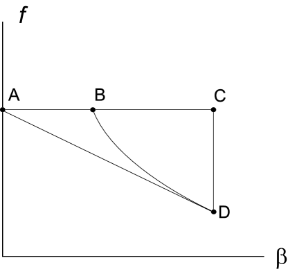
Figure 1: Two regions ($ABD$ and $BCD$) in the plane of parameters $(f,\beta)$ where the Friedmann singularity is stable are shown. For each fixed value of parameter $\gamma$ the coordinates of the points $A,B,C,D$ are fixed and all acceptable values of $f,\beta$ for each $\gamma$ are located in the region $ABCD.$ In $ABD$ both exponents $s_{1}$ and $s_{2}$ are real and positive and at the same time no supraluminal velocities exists. In $BCD$ exponents $s_{1}$ and $s_{2}$ are complex conjugated to each other but with the positive real part and again no supraluminal signals exist. The coordinates of the boundary points $A,B,C,D$ depend on the constant $\gamma$ (which has been chosen from the region $1\leqslant\gamma<2$) and they are (the first coordinate indicate the value of $f$ and the second  the value of $\beta)$: $A[\frac{3}{4}\gamma(2-\gamma),$ $0],$ $B[\frac{3}{4}\gamma(2-\gamma),\frac{2+\gamma-\sqrt{8\gamma(2-\gamma)}}{\gamma}],$ $C[\frac{3}{4}\gamma(2-\gamma),$ $\frac{3\gamma-2}{\gamma}],$ $D[\frac{3}{8}\left(2-\gamma\right)^{2},$ $\frac{3\gamma-2}{\gamma}].$ The straight line $AD$ has the equation $f=\frac{3}{8}\gamma\left(2-\gamma\right)(2-\beta).$ The curve $BD$ is the piece of parabola $f=$ $\frac{3}{32}\left[2-\gamma\left(\beta-1\right)\right]^{2}.$

Fom the first of the equations (39) follows amplitude $A$:

$$A=q_{1}C_{\lambda}^{\left(1\right)}t^{s_{1}-2}+q_{2}C_{\lambda}^{\left(2\right)}t^{s_{2}-2},$$ (57)

where

$$q_{1}=\frac{s_{1}\left(\gamma s_{1}-\gamma+2\right)}{2\gamma}\text{ },\text{ \ }q_{2}=\frac{s_{2}\left(\gamma s_{2}-\gamma+2\right)}{2\gamma}\text{ }.$$ (58)

Now one can make asymptotics for $\lambda,\mu$ and $A$ more precise taking into account those terms in equations (24)- (26) containing the factor $k^{2}R^{-2}$, that is the terms which have been neglected in the first approximation. Analysis shows that their influence consists in generation the small time-dependent corrections to the arbitrary constants appeared in the first approximation. These corrections are completely expressible in terms of parameters of the first approximation, that is they do not bring any new arbitrariness in the solution. The fact is that the exact general solution of equations (24)- (26) for the functions $\lambda,\mu$ and $t^{2}A$ has the form $F^{\left(0\right)}\left(t\right)+t^{s_{1}}F^{\left(1\right)}\left(t\right)+t^{s_{2}}F^{\left(2\right)}\left(t\right)$ with the same exponents $s_{1}$ and $s_{2}$ given by the formula (54) and with functions $F^{\left(0\right)},F^{\left(1\right)},F^{\left(2\right)}$ each of which can be expressed in the form of the Taylor series in the small parameter $\zeta$:

$$\zeta=\left(kt/R\right)^{2},$$ (59)

which parameter tends to zero in the limit $t\rightarrow 0$ because $\left(kt/R\right)^{2}=k^{2}t_{c}^{4/3\gamma}t^{2\left(3\gamma-2\right)/3\gamma}$ and $\gamma\geqslant 1$. The first time-independent terms in these power series are just the arbitrary constants figured in the formulas (42),(53) and (57). The general structure of the exact solution for $\lambda,\mu$ and $t^{2}A$ is:

$$\lambda =\left(C_{\lambda}^{\left(0\right)}+\alpha_{\lambda 1}^{\left(0\right)}\zeta+\alpha_{\lambda 2}^{\left(0\right)}\zeta^{2}...\right)+$$ (60)

$$+\left(C_{\lambda}^{\left(1\right)}+\alpha_{\lambda 1}^{\left(1\right)}\zeta+\alpha_{\lambda 2}^{\left(1\right)}\zeta^{2}...\right)t^{s_{1}}+$$

$$+\left(C_{\lambda}^{\left(2\right)}+\alpha_{\lambda 1}^{\left(2\right)}\zeta+\alpha_{\lambda 2}^{\left(2\right)}\zeta^{2}...\right)t^{s_{2}},$$

$$\mu =\left(C_{\mu}^{\left(0\right)}+\alpha_{\mu 1}^{\left(0\right)}\zeta+\alpha_{\mu 2}^{\left(0\right)}\zeta^{2}...\right)+$$ (61)

$$+\left(\alpha_{\mu 1}^{\left(1\right)}\zeta+\alpha_{\mu 2}^{\left(1\right)}\zeta^{2}...\right)t^{s_{1}}+$$

$$+\left(\alpha_{\mu 1}^{\left(2\right)}\zeta+\alpha_{\mu 2}^{\left(2\right)}\zeta^{2}...\right)t^{s_{2}},$$

$$t^{2}A =\left(\alpha_{A1}^{\left(0\right)}\zeta+\alpha_{A2}^{\left(0\right)}\zeta^{2}...\right)+$$ (62)

$$+\left(q_{1}C_{\lambda}^{\left(1\right)}+\alpha_{A1}^{\left(1\right)}\zeta+\alpha_{A2}^{\left(1\right)}\zeta^{2}...\right)t^{s_{1}}+$$

$$+\left(q_{2}C_{\lambda}^{\left(2\right)}+\alpha_{A1}^{\left(2\right)}\zeta+\alpha_{A2}^{\left(2\right)}\zeta^{2}...\right)t^{s_{2}},$$

where all $\alpha$-coefficients in front of the powers of parameter $\zeta$ are constant quantities which depend on the four arbitrary constants $C_{\mu}^{\left(0\right)},C_{\lambda}^{\left(0\right)},C_{\lambda}^{\left(1\right)},C_{\lambda}^{\left(2\right)}$ and external numbers $f,\beta,\gamma$. There is no big sense in taking into account corrections containing the powers of $\zeta$ in the factors in front of the powers $t^{s_{1}}$ and $t^{s_{2}}$ since this would give the small unimportant addends to the asymptotics. The same is true for the corrections of the orders $\zeta^{2}$ and higher in terms which do not contain powers $t^{s_{1}}$ and $t^{s_{2}}$. However, to keep the terms $\alpha_{\lambda 1}^{\left(0\right)}\zeta$ , $\alpha_{\mu 1}^{\left(0\right)}\zeta$ and $\alpha_{A1}^{\left(0\right)}\zeta$ in the asymptotics is necessary because in general they, although small, play a role in the behaviour of the solution and the first non-vanishing term in the asymptotic expression for the energy density depends on them. Calculations gives the following result for the coefficients $\alpha_{\lambda 1}^{\left(0\right)},\alpha_{\mu 1}^{\left(0\right)}$ and $\alpha_{A1}^{\left(0\right)}$:

$$a_{\lambda 1}^{\left(0\right)}=\frac{3\gamma^{2}\left(3\gamma\beta-4\right)}{2\left(3\gamma-2\right)\left[24f+\left(3\gamma+2\right)\left(3\gamma\beta-4\right)\right]}\left(C_{\lambda}^{\left(0\right)}+C_{\mu}^{\left(0\right)}\right),$$ (63)

$$a_{\mu 1}^{\left(0\right)}=-\frac{3\gamma^{2}}{2\left(9\gamma-4\right)}\left(C_{\lambda}^{\left(0\right)}+C_{\mu}^{\left(0\right)}\right),$$ (64)

$$a_{A1}^{\left(0\right)}=-\frac{4f}{24f+\left(3\gamma+2\right)\left(3\gamma\beta-4\right)}\left(C_{\lambda}^{\left(0\right)}+C_{\mu}^{\left(0\right)}\right).$$ (65)

Then the final sufficient asymptotics for the amplitudes $\lambda,\mu$ and $A$ is:

$$\lambda=C_{\lambda}^{\left(0\right)}+C_{\lambda}^{\left(1\right)}t^{s_{1}}+C_{\lambda}^{\left(2\right)}t^{s_{2}}+\alpha_{\lambda 1}^{\left(0\right)}k^{2}t_{c}^{4/3\gamma}t^{s_{3}},$$ (66)

$$\mu=C_{\mu}^{\left(0\right)}+\alpha_{\mu 1}^{\left(0\right)}k^{2}t_{c}^{4/3\gamma}t^{s_{3}},$$ (67)

$$A=q_{1}C_{\lambda}^{\left(1\right)}t^{s_{1}-2}+q_{2}C_{\lambda}^{\left(2\right)}t^{s_{2}-2}+\alpha_{A1}^{\left(0\right)}k^{2}t_{c}^{4/3\gamma}t^{s_{3}-2}.$$ (68)

where

$$s_{3}=\frac{2\left(3\gamma-2\right)}{3\gamma}$$ (69)

The exact coincidence of the forms of equations (39)-(41) means that in the main approximation the other pairs of amplitudes $\sigma_{\left(J\right)},B_{\left(J\right)}$ and $\omega_{\left(J\right)},D_{\left(J\right)}$ are described by the same formulas (53)-(54) and (57)-(58) with only difference that instead of $C_{\lambda}^{\left(0\right)},C_{\lambda}^{\left(1\right)},C_{\lambda}^{\left(2\right)}$ one should take the new arbitrary constants $C_{\sigma_{\left(J\right)}}^{\left(0\right)},C_{\sigma_{\left(J\right)}}^{\left(1\right)},C_{\sigma_{\left(J\right)}}^{\left(2\right)}$ and $C_{\omega_{\left(J\right)}}^{\left(0\right)},C_{\omega_{\left(J\right)}}^{\left(1\right)},C_{\omega_{\left(J\right)}}^{\left(2\right)}$ respectively. After that one can calculate corrections to this main approximation taking into account the influence of the terms in equations (27)-(30) containing the factor $k^{2}R^{-2}.$ These calculations are analogous to those we made for the amplitudes $\lambda,\mu,t^{2}A$ and the final results are:

$$\sigma_{\left(J\right)}=C_{\sigma_{\left(J\right)}}^{\left(0\right)}+C_{\sigma_{\left(J\right)}}^{\left(1\right)}t^{s_{1}}+C_{\sigma_{\left(J\right)}}^{\left(2\right)}t^{s_{2}},\text{ \ }$$ (70)

$$\omega_{\left(J\right)}=C_{\omega_{\left(J\right)}}^{\left(0\right)}+C_{\omega_{\left(J\right)}}^{\left(1\right)}t^{s_{1}}+C_{\omega_{\left(J\right)}}^{\left(2\right)}t^{s_{2}}+\alpha_{\omega_{\left(J\right)}1}^{\left(0\right)}k^{2}t_{c}^{4/3\gamma}t^{s_{3}},\text{ }$$ (71)

$$B_{\left(J\right)}=q_{1}C_{\sigma_{\left(J\right)}}^{\left(1\right)}t^{s_{1}-2}+q_{2}C_{\sigma_{\left(J\right)}}^{\left(2\right)}t^{s_{2}-2},$$ (72)

$$D_{\left(J\right)}=q_{1}C_{\omega_{\left(J\right)}}^{\left(1\right)}t^{s_{1}-2}+q_{2}C_{\omega_{\left(J\right)}}^{\left(2\right)}t^{s_{2}-2}+\alpha_{D_{\left(J\right)}1}^{\left(0\right)}k^{2}t_{c}^{4/3\gamma}t^{s_{3}-2},$$ (73)

where the coefficients $\alpha_{\omega_{\left(J\right)}1}^{\left(0\right)}$ and $\alpha_{D_{\left(J\right)}1}^{\left(0\right)}$ are:

$$\alpha_{\omega_{\left(J\right)}1}^{\left(0\right)}=-\frac{9\gamma^{2}\left(3\gamma\beta-4\right)}{2\left(3\gamma-2\right)\left[24f+\left(3\gamma+2\right)\left(3\gamma\beta-4\right)\right]}C_{\omega_{\left(J\right)}}^{\left(0\right)}\text{ },$$ (74)

$$\alpha_{D_{\left(J\right)}1}^{\left(0\right)}=-\frac{12f}{24f+\left(3\gamma+2\right)\left(3\gamma\beta-4\right)}C_{\omega_{\left(J\right)}}^{\left(0\right)}\text{ }.$$ (75)

Due to specific structure of equations (27) and (28) the solutions for perturbations $\sigma_{\left(J\right)},$ $t^{2}B_{\left(J\right)}$ do not contain corrections of the order $t^{s_{3}}$.

The two arbitrary constants $C_{\sigma_{\left(J\right)}}^{\left(0\right)}$ can be removed by the coordinate transformations which still remain in the synchronous system (in addition to those by which we already eliminated constant $C_{\mu}^{\left(-1\right)}$ and can eliminate constant $C_{\mu}^{\left(0\right)}$ in function $\mu$). Consequently the total number of the arbitrary physical constants in the Fourier coefficients (which generate the arbitrary 3-dimensional physical function in the real $x$-space) of the solution is 13, these are $C_{\lambda}^{\left(0\right)},C_{\lambda}^{\left(1\right)},C_{\lambda}^{\left(2\right)},$ $C_{\sigma_{\left(J\right)}}^{\left(1\right)},C_{\sigma_{\left(J\right)}}^{\left(2\right)},C_{\omega_{\left(J\right)}}^{\left(0\right)},C_{\omega_{\left(J\right)}}^{\left(1\right)},C_{\omega_{\left(J\right)}}^{\left(2\right)}$. This is exactly the number of arbitrary independent physical degrees of freedom of the system under consideration, that is 4 for the gravitational field, 1 for the energy density, 3 for the velocity and 5 for the shear stresses (five because the six components $S_{\alpha\beta}$ follows from the six differential equations of the first order in time with one additional condition $\delta^{\alpha\beta}S_{\alpha\beta}=0$). Then the solution we constructed is generic.

The asymptotic solutions for the Fourier coefficients for perturbations of the velocity and energy density follow from (31)-(32):

$$\tilde{V}_{\alpha} =\frac{3ik\gamma}{8}\left(\frac{2k_{\alpha}}{3k}C_{\lambda}^{\left(1\right)}-\sum_{J=2}^{3}l_{\alpha}^{\left(J\right)}C_{\sigma_{\left(J\right)}}^{\left(1\right)}\right)s_{1}t^{s_{1}+1}+$$ (76)

$$+\frac{3ik\gamma}{8}\left(\frac{2k_{\alpha}}{3k}C_{\lambda}^{\left(2\right)}-\sum_{J=2}^{3}l_{\alpha}^{\left(J\right)}C_{\sigma_{\left(J\right)}}^{\left(2\right)}\right)s_{2}t^{s_{2}+1}+$$

$$+\frac{ik_{\alpha}\left(3\gamma-2\right)}{6}\left(\alpha_{\lambda 1}^{\left(0\right)}+\alpha_{\mu 1}^{\left(0\right)}\right)k^{2}t_{c}^{4/3\gamma}t^{s_{3}+1},$$

$$\tilde{E}=\frac{\gamma}{9\gamma-4}\left(C_{\lambda}^{\left(0\right)}+C_{\mu}^{\left(0\right)}\right)k^{2}t_{c}^{4/3\gamma}t^{s_{3}-2}.$$ (77)

It is evident that the asymptotic behaviour of all perturbations satisfy the basic requirement to be small in relative sense. This condition means that variations (12) must be small with respect to the corresponding background values, that is the quantities $\frac{\delta g_{\alpha\beta}}{R^{2}},\frac{\delta\varepsilon}{\varepsilon},\delta u_{\alpha}$ and $\frac{\delta S_{\alpha\beta}}{\varepsilon R^{2}}$ in the limit $t\rightarrow 0$ should be much less than unity (the necessity to be small for the last ratio follows from the condition $\delta S_{\alpha\beta}\ll T_{\alpha\beta}^{\left(0\right)}=pg_{\alpha\beta}^{\left(0\right)}\sim\varepsilon R^{2}$). In terms of the Fourier amplitudes these requirements are $\tilde{H}_{\alpha\beta}\ll 1,$ $t^{2}\tilde{E}\ll 1,$ $\tilde{V}_{\alpha}\ll 1,$ $t^{2}\tilde{K}_{\alpha\beta}\ll 1$ and all of them are satisfied since all time-dependent terms in the left hand sides of these inequalities are going to die away as $t\rightarrow 0$ and the six arbitrary constants

$$\tilde{H}_{\alpha\beta}^{\left(0\right)}=C_{\lambda}^{\left(0\right)}P_{\alpha\beta}\text{ }+C_{\mu}^{\left(0\right)}Q_{\alpha\beta}+{\displaystyle\sum\limits_{J=2}^{3}}\left[C_{\sigma_{\left(J\right)}}^{\left(0\right)}L_{\alpha\beta}^{\left(J\right)}+C_{\omega_{\left(J\right)}}^{\left(0\right)}G_{\alpha\beta}^{\left(J\right)}\right]$$ (78)

in the metric perturbations $\tilde{H}_{\alpha\beta}$ we are free to take to be infinitesimally small. The interpretation of these constants is well known: their appearance simply indicates that the isotropic part of the perturbed metric $g_{\alpha\beta}$ in the $x$-space instead of the seed value $R^{2}\delta_{\alpha\beta}$ acquires the more general form $R^{2}a_{\alpha\beta}\left(x^{1},x^{2},x^{3}\right)$ where $a_{\alpha\beta}$ in perturbative solution should be closed to $\delta_{\alpha\beta}$ but in the non-perturbative context (see below) becomes an arbitrary symmetric 3-dimensional tensor.

All this means that in the real $x$-space a generic non perturbative solution exists with the following asymptotics for the metric near singularity:

$$g_{\alpha\beta}=R^{2}\left(a_{\alpha\beta}+t^{s_{1}}b_{\alpha\beta}^{\left(1\right)}+t^{s_{2}}b_{\alpha\beta}^{\left(2\right)}+t^{s_{3}}b_{\alpha\beta}^{\left(3\right)}+...\right)$$ (79)

where $R=\left(t/t_{c}\right)^{2/3\gamma}$ and exponents $s_{1},s_{2}$ and $s_{3}$ are defined by the relation (54) and (69). The additional terms denoted by the triple dots are small corrections which contain the terms of the orders $t^{2s_{3}},t^{s_{1}+s_{3}},$ $t^{s_{2}+s_{3}}$ as well as all their powers and cross products. The main addend $a_{\alpha\beta}$ represents six arbitrary 3-dimensional functions (in the linearized version they are generated by the arbitrary constants $C_{\lambda}^{\left(0\right)},C_{\mu}^{\left(0\right)},C_{\sigma_{\left(J\right)}}^{\left(0\right)},C_{\omega_{\left(J\right)}}^{\left(0\right)}$ in the Fourier coefficients). Each tensor $b_{\alpha\beta}^{\left(1\right)}$ and $b_{\alpha\beta}^{\left(2\right)}$ consists of the six 3-dimensional functions subjected to the restrictions $a^{\alpha\beta}b_{\alpha\beta}^{\left(1\right)}=0$ and $a^{\alpha\beta}b_{\alpha\beta}^{\left(2\right)}=0$ (here $a^{\alpha\beta}$ is inverse to $a_{\alpha\beta}$), consequently $b_{\alpha\beta}^{\left(1\right)}$ and $b_{\alpha\beta}^{\left(2\right)}$ contain another ten arbitrary 3-dimensional functions (in the linearized version they are generated by the ten arbitrary constants $C_{\lambda}^{\left(1\right)},C_{\lambda}^{\left(2\right)},C_{\sigma_{\left(J\right)}}^{\left(1\right)},C_{\sigma_{\left(J\right)}}^{\left(2\right)},C_{\omega_{\left(J\right)}}^{\left(1\right)},C_{\omega_{\left(J\right)}}^{\left(2\right)}$ in the Fourier coefficients). In case of complex conjugated $s_{1}$ and $s_{2}$ the components $b_{\alpha\beta}^{\left(1\right)}$ and $b_{\alpha\beta}^{\left(2\right)}$ are complex but in the way to provide reality of the metric tensor. The last term $b_{\alpha\beta}^{\left(3\right)}$ and all corrections denoted by the triple dots in the expansion (79) are expressible in terms of the $a_{\alpha\beta},b_{\alpha\beta}^{\left(1\right)},b_{\alpha\beta}^{\left(2\right)}$ and their derivatives then they do not contain any new arbitrariness. The shear stresses, velocity and energy density follows from the exact Einstein equations in terms of the metric tensor (79) and its derivatives and all these quantities also do not contain any new arbitrary parameters. In result the solution contains 16 arbitrary 3-dimensional functions the three of which represent the gauge freedom due to the possibility of the arbitrary 3-dimensional coordinate transformations. Then the physical freedom in the solution corresponds to 13 arbitrary functions as it should be.

This result is the generalization of the so-called quasi-isotropic solution constructed in LK2 (see also LK ) for the perfect liquid. However, in case of perfect liquid the isotropic singularity is unstable and asymptotics found in LK2 corresponds to the narrow class of particular solutions containing only 3 arbitrary physical 3-dimensional parameters.

V Concluding remarks

1. The results presented show that the viscoelastic material with shear viscosity coefficient $\eta\sim\sqrt{\varepsilon}$ can stabilize the Friedmann cosmological singularity and the corresponding generic solution of the Einstein equations for the viscous fluid possessing the isotropic Big Bang (or Big Crunch) exists. Depending on the free parameters $f,\beta,\gamma$ of the theory such solution can be either of smooth power law asymptotics near singularity (when both power exponents $s_{1}$ and $s_{2}$ are real and positive) or it can have the character of damping (in the limit $t\rightarrow 0$) oscillations (when $s_{1}$ and $s_{2}$ have the positive real part and an imaginary part). The last possibility reveals itself as a weak trace of the chaotic oscillatory regime which is characteristic for the most general asymptotics near the cosmological singularity and which can not be described in closed analytical form (for the short simplified review on the oscillatory regime see Bel1 ). The present case show that the shear viscosity can smooth such chaotic behaviour up to the quiet oscillations which have simple asymptotic expressions in terms of the elementary functions of the type $t^{\operatorname{Re}s}\sin\left[\left(\operatorname{Im}s\right)\ln t\right]$ and $t^{\operatorname{Re}s}\cos\left[\left(\operatorname{Im}s\right)\ln t\right].$

2. In the generic isotropic Big Bang described here some part of perturbations are presented already at the initial singularity $t=0$ which are the three physical components of the arbitrary 3-dimensional tensor $a_{\alpha\beta}(x^{1},x^{2},x^{3})$ in formula (79). Another ten arbitrary physical degrees of freedom are contained in the components of two tensors $b_{\alpha\beta}^{\left(1\right)}$ and $b_{\alpha\beta}^{\left(2\right)}$ in this formula and they come to the action in the process of expansion. This picture has no that shortage of the classical Lifshitz approach when one is forced to introduce some unexplainable segment between singularity $t=0$ and initial time $t=t_{0}$ when perturbations arise in such a way that inside this segment it is necessary to postulate without reasons the validity of the exact Friedmann solution free of any perturbations.

3. It might happen that due to the universal growing of all perturbations (in the course of expansion) already before that critical time when equations of state will be changed and will switched off the action of viscosity the perturbation amplitudes will reach the level sufficient for the further development of the observed structure of our Universe. If not we always have that means of escape as inflation phase which can be inserted in the evolution after the Big Bang. Here we are touching another problem. It is known Vil ; Bor that no inflation (including ”eternal” one) can appear without preceding cosmological singularity. Moreover, namely the period of expansion from singularity to inflationary stage is responsible for the generation of the necessary initial conditions for the such inflationary phase. How to match the singular and inflationary stages and to find the initial conditions for inflation call for another good piece of work.

4. In our analysis the case of stiff matter ($\gamma=2$) have been excluded. This peculiar possibility should be investigated separately. It is known that for the perfect liquid with stiff matter equation of state a generic solution with isotropic singularity is impossible (see Bel1 and references therein). The asymptotic of the general solution for this case have essentially anisotropic structure although of the smooth (non-oscillatory) power law character. It might be that viscosity will be able to isotropize such evolution, however, it is not yet clear how the viscous stiff matter should be treated mathematically. The simple way to take $\gamma=2$ in our previous study does not works.

5. Another interesting question is how an evolution directed outwards of a thermally equilibrated state to a non-equilibrium one can be reconciled with the second law of thermodynamics. Indeed, it seems that in accordance with this law no deviation can happen from the background Friedmann expansion since in course of a such deviation entropy must increase but in equilibrium it already has the maximal possible value. The explanation should come from the fact of the presence of the superstrong gravitational field. This field is an external agent with respect to the matter itself, consequently, the matter in the Friedmann Universe cannot be consider as closed system. It might happen that Penrose Pen is right and the gravitational field possess an intrinsic entropy then this entropy being added to the entropy of matter will bring the situation to the normal one. To clarify the question let’s calculate the matter entropy production near singularity in the solution described in the previous sections. For the energy-momentum tensor (1)-(2) equation $T_{i;k}^{k}u^{i}=0$ can be written as

$$\left(\sigma u^{k}\right)_{;k}=-T^{-1}S^{mn}u_{m;n}\text{ },$$ (80)

where $\sigma$ and $T$ is the entropy density and temperature of a (perturbed) fluid. Here we used the fact that in our model chemical potential vanish (that is $\gamma\varepsilon=T\sigma$) and that principal assumption of the Israel-Stewart theory that the Gibbs relation (in our case $d\varepsilon=Td\sigma$) is universal in the sense that it is valid for the arbitrary displacements of the thermodynamical parameters, that is not only between neighbouring equilibrium states. Equation (4) for stresses being multiplied by $S^{ik}$ gives:

$$S^{mn}u_{m;n}=-\frac{\tau}{2\eta}\left[\frac{1}{2}\left(S^{mn}S_{mn}\right)_{;k}u^{k}+\frac{1}{\tau}S^{mn}S_{mn}\right].$$ (81)

Substituting this into the previous formula we obtain:

$$\left(\sigma u^{k}-\frac{\tau}{4\eta T}S^{mn}S_{mn}u^{k}\right)_{;k}=$$ (82)

$$=\frac{1}{2\eta T}S^{mn}S_{mn}-\left(\frac{\tau}{4\eta T}u^{k}\right)_{;k}S^{mn}S_{mn}$$

The 4-vector in the brackets in the left hand side of the last equation represents the generalization of the Landau-Lifshitz entropy flux for the case when relaxation time $\tau$ of the shear stresses is not zero. This expression for the entropy flux is the same that have been proposed by the Israel-Stewart theory Isr1 ; Isr2 .

If the background solution is an real equilibrium state in the literal sense then the action of the operator $u^{k}\partial_{k}$ on the background values of quantities $\tau,\eta,T$ gives zero and also $u_{;k}^{k}=0$ for the background values of the 4-velocity. Then the factor $\left(\tau u^{k}/4\eta T\right)_{;k}$ in front of $S^{mn}S_{mn}$ in the last term of the equation (82) disappears in the first approximation. Then this last term belongs to the third approximation since also $S^{mn}$ vanish for the background solution. Consequently up to the second order in the deviation from the equilibrium the equation (82) provides correct result, that is for any future directed evolution the entropy increases because the quantity $S^{mn}S_{mn}$ is always positive due to the properties (2) of the stresses.

However, the Friedmann background is not an equilibrium state in the aforementioned literal sense. This solution describes the quasi-stationary evolution in which the Universe passes the continuous sequence of equilibrium states with different equilibrium parameters but with one and the same conserved entropy. Due to this evolution the background value of the factor $\left(\tau u^{k}/4\eta T\right)_{;k}$ in equation (82) is not zero, moreover, it is not small with respect to the factor $1/2\eta T$ in the first term in the right hand side of the equation (82). It is easy to get $\left(\tau u^{k}/4\eta T\right)_{;k}$ from formulas (10)-(11) and (51) using expression $T=\gamma\varepsilon_{c}\left(\varepsilon/\varepsilon_{c}\right)^{\left(\gamma-1\right)/\gamma}$ for the background temperature ($\varepsilon_{c}$ is an arbitrary constant). In result the entropy production equation (82) for our model take the form

$$\left(\sigma u^{k}-\frac{\tau}{4\eta T}S^{mn}S_{mn}u^{k}\right)_{;k}=\frac{\beta-2}{2\beta\eta T}S^{mn}S_{mn}\text{ },$$ (83)

and one can see that constant $\beta-2$ is negative. Indeed, the first inequality in both sets of stability conditions (55) and (56) is $\beta<\left(3\gamma-2\right)/\gamma$ but for any value of parameter $\gamma$ from the interval $1\leqslant\gamma<2$ the quantity $\left(3\gamma-2\right)/\gamma$ is less than $2$.

It might be thought that the negativity of the right hand side of equation (83) means that the second law of thermodynamics precludes the physical realization of the generic isotropic Big Bang. However, it can happen that such conclusion again would be too hasty because, as we already said, the entropy of gravitational field might normalize the situation. As of now no concrete calculation can be made inasmuch no theory of the gravitational entropy exists. Nevertheless in the model under investigation it looks plausible that gravitational entropy, being proportional to some invariants of the Weyl tensor Pen , indeed would be able to change the state of affairs because for the background Friedmann solution this tensor is identically zero and it will start to increase in the course of expansion. Then increasing of the gravitational entropy would compensate the decreasing of the matter entropy. For those who believe that the Universe began by an isotropic expansion the negativity of the right hand side of the equation (83) stands as a hint that gravitational entropy indeed exists.

By the way it is worth to remark that practically in all publications (including Isr1 ; Isr2 ) dedicated to the extended thermodynamics in the framework of the General Relativity the condition $\sigma_{;k}^{k}\geqslant 0$ for the entropy flux of the matter is accepted from the beginning as one’s due. Moreover, namely from this condition follows the structure of the additional dissipative terms in the energy-momentum tensor and particle flux. Such strategy is undoubtedly correct not only for the ”everyday life” but also for the majority of the astrophysical problems where the gravitational fields are relatively weak. However the cases with extremely strong gravity as in vicinity to the cosmological singularity need more precise definition of what we should understand under the total entropy of the system.

VI Acknowledgements

It is a pleasure to thank G.Bisnovatiy-Kogan for the useful critics and stimulating discussions and E.Vladimirova for the help which accelerates the creation of the final version of the manuscript.

References

• (1) J.D.Barrow and R.A.Matzner ”The homogeneity and isotropy of the Universe”, Mon. Not. R. astr. Soc., 181, 719 (1977).
• (2) R.Penrose ”Singularities and Time-Asymmetry”, General Relativity: An Einstein Centenary Survey, Cambridge University Press, 581 (1979).
• (3) S.W.Goode, A.A.Coley and J.Wainwright  ”The isotropic singularity in cosmology”, Class. Quant.   Grav.,9, 445 (1992).
• (4) C.Eckart ”The Thermodynamics of Irreversible Processes III. Relativistic Theory of the Simple Fluid”, Phys. Rev., 58, 919 (1940).
• (5) L.D.Landau and E.M.Lifschitz, Fluid Mechanics, Addison Wesley, Reading, Mass. (1958).
• (6) C.Cattaneo ”Sur une forme de l’équation de la chaleur éliminant le paradoxe d’une propagation instantanée”, Comptes rendus Acad. Sci. Paris Sér. A-B, 247, 431 (1958). Based on his earlier seminar talk ”Sulla conduzione del calore”, Atti Semin. Mat. Fis. Univ. Modena, 3, 83 (1948).
• (7) W.Israel ”Nonstationary Irreversible Thermodynamics: A Causal Relativistic Theory”, Ann. Phys., 100, 310 (1976).
• (8) W.Israel and J.M.Stewart ”Transient Relativistic Thermodynamics and Kinetic Theory”, Ann. Phys., 118, 341 (1979).
• (9) V.A.Belinski, E.S.Nikomarov and I.M.Khalatnikov ”Investigation of the cosmological evolution of viscoelastic matter with causal thermodynamics”, Sov.Phys. JETP, 50, 213 (1979).
• (10) E.M.Lifschitz ”On the gravitational stability of the expanding universe””, ZhETP, 16, 587 (1946) (in russian); reprinted: Journal of Physics (USSR), 10, 116 (1946).
• (11) E.M.Lifschitz and I.M.Khalatnikov ”Problems of Relativistic Cosmology”, Soviet Physics Uspekhi, 6, 495 (1964).
• (12) I.S.Gradshteyn and I.M.Ryzhik ”Table of Integrals, Series, and Products”, Section 9, A.Jeffrey and D.Zwillinger (eds.), 2007.
• (13) R.Geroch and L.Lindblom ”Dissipative relativistic fluid theories of divergence type”, Phys.Rev., D41, 1855 (1990).
• (14) W.Hiscock and L.Lindblom ”Generic instabilities in first-order dissipative relativistic fluid theories”, Phys.Rev.D, 31, 725 (1985).
• (15) E.M.Lifschitz and I.M.Khalatnikov ”On the singularities of cosmological solutions of the gravitational equations.I”, Sov.Phys. JETP, 12, 108 (1961).
• (16) V.Belinski ”Cosmological singularity”, arXiv:0910.0374, [gr-qc].
• (17) A.Vilenkin ”Did the Universe have a beginning?”, Phys.Rev., D46, 2355 (1992).
• (18) A.Borde, A.Guth and A.Vilenkin ”Inflationary spacetimes are not past-complete”, Phys.Rev.Lett., 90, 151301 (2003).
• (1)