Orientational glass in mixtures of elliptic and circular particles:
Structural heterogeneities, rotational dynamics, and rheology

Abstract

Using molecular dynamics simulation with an angle-dependent Lennard-Jones potential, we study orientational glass with quadrupolar symmetry in mixtures of elliptic particles and circular impurities in two dimensions. With a mild aspect ratio ($=1.2$) and a mild size ratio ($=1.2$), we realize a plastic crystal at relatively high temperature $T$. With further lowering $T$, we find a structural phase transition for very small impurity concentration $c$ and pinned disordered orientations for not small $c$. The ellipses are anchored by the impurities in the planar alignment. With increasing $c$, the orientation domains composed of isosceles triangles gradually become smaller, resulting in orientational glass with crystal order. In our simulation, the impurity distribution becomes heterogeneous during quenching from liquid, which then produces rotational dynamic heterogeneities. We also examine rheology in orientational glass to predict a shape memory effect and a superelasticity effect, where a large fraction of the strain is due to collective orientation changes.

I Introduction

Certain anisotropic molecules such as KCN, N₂ and ortho-H form a cubic crystal without orientational order ori ; Binder ; Kob-Binder . Solids in such a rotator phase are often called plastic solids Sherwood . As the temperature $T$ is further lowered, they undergo orientational phase transitions, where the crystal structure changes from a cubic to noncubic one St ; ori . In mixtures of anisotropic particles such as KCN diluted with KBr, N₂ diluted with Ar, and ortho-H diluted with para-H, the so-called orientational glass is realized with increasing the impurity concentration $c$ ori ; Binder ; Kob-Binder , where the quadrupolar, orientational degrees of freedom are randomly frozen Sullivan . In such mixtures, a specific-heat peak ori ; Mertz and a decrease in one of the shear moduli ori ; sound have been observed above the transition for not large $c$. The latter indicates a strong orientation-strain coupling Raedt ; Knorr ; Bell ; Harris . To explain these behaviors, molecular dynamics (MD) simulation was also performed on mixed cyanides Klein . It is also remarkable that one-component systems of globular molecules such as ethanol, cyclohexanol, and C₆₀ have rotator phases and are orientationally arrested at lower $T$ with weak specific-heat singularities Seki ; Yamamuro ; C60 .

However, not enough attention has yet been paid to the physics of orientational glass. In contrast, numerous investigations have been made on translational glass, where positional disorder is frozen Kob-Binder . In previous MD simulations on diatomic systems Kob1 and more complex molecular systems Lewis , the correlations between the translational and rotational degrees of freedom have been examined in glassy states. Glassy dynamics was also found in monodisperse hard ellipsoids with a slight anisotropy Schilling . Moreover, in double glass Sch , these two kinds of degrees of freedom have been predicted to freeze at the same temperature.

Recently, we performed MD simulation on mixtures of spheroidal particles and spherical impurities in three dimensions to examine the formation of orientational glass EPL . In this paper, we aim to investigate its complex dynamics in more detail in mixtures of elliptic particle and circular impurities in crystal in two dimensions. We assume a mild aspect ratio ($=1.2$) of the ellipses to avoid liquid crystal mesophases and a mild size ratio ($=1.2$) between the two species to suppress positional disorder. We vary $T$ and $c$ to examine the changeover between multi-variant domain states for small $c$ and highly frustrated states of orientational glass for not small $c$. We shall find that mesoscopic orientational order and strains exist in glassy states. Previously, for binary mixtures of circular particles, the changeover between polycrystal and translational glass was studied with varying $c$ Hamanaka . In translational glass, mesoscopic crystalline order still remains and was visualized Hamanaka ; Tanaka . In double glass, simultaneous appearance of these two mesoscopic heterogeneities have been detected Takae-double .

If the molecules forming a crystal are anisotropic, there arises a direct coupling between the orientations and the lattice deformations Raedt ; Knorr ; Bell ; Harris . In fact, an effective interaction mediated by acoustic phonons was derived among anisotropic particles in crystal such as (CN)^- in KCN Raedt ; Knorr ; Bell , leading to acoustic softening in the rotator phase ori ; sound . The orientational phase transitions for small $c$ thus belong to type-I instabilities in Cowley’s classification of elastic instabilities Cowley ; Onukibook , where acoustic modes become soft in particular wave vector directions. In this paper, we predict shape memory effect and a superelasticity effect in orientational glass at low $T$, where favored oriented domains increase and disfavored ones decrease upon stretching. These effects are well-known for shape-memory alloys such as TiNi marten ; RenReview ; Ren . Molecular dynamics simulation was also performed to reproduce superelasticity for a model alloy Suzuki . It is worth noting that mesoscopic strain heterogeneities were observed in TiNi glass, which were on a scale of $20$nm at a slightly off-stoichiometric composition Ren .

As another ingredient, we shall find a tendency of impurity clustering depending on the molecular interactions EPL . In our simulation, it took place during quenching from high-temperature liquid to low-temperature solid. The impurity clustering gives rise to significant heterogeneities in orientational order and rotational dynamics. For example, a small fraction of the elliptic particles remain not strongly anchored to the impurities such that they undergo flip rotations even at very low $T$. Though such effects have rarely been discussed in the literature, they should be relevant in many real experiments.

We point out that our system is similar to liquid crystal gels (gels containing rodlike molecules) PGgel ; Tere . In such soft matter, there arises a strong orientation-strain coupling, which makes the isotropic-nematic transition analogous to the orientation transition in solids. Irregularities in the crosslinkage play the role of random quenched disorder, leading to mesoscopic nematic polydomains Uchida . Application of stress or electric field induces polydomain-monodomain transitions Kai . We also note that dilute magnetic alloys, called spin glass, have glassy phases characterized by frozen-in local magnetic moments which point in random directions Binder ; Sullivan ; Kob-Binder . However, in its research, the spin-lattice coupling and the impurity clustering (resulting in correlated quenched disorder) have not yet been well examined.

The problem of orientational glass is thus closely related to many important problems in solids and soft matter. On the basis of a simple microscopic model, we organize this paper as follows. In Sec.II, we will present the background of our simulation. In Sec.III, we will display orientational configurations for various $c$ at low $T$. In Sec.IV, we will examine the rotational dynamics. In Sec.V, we will treat rheology of orientational glass.

II Simulation background

We use an angle-dependent potential EPL , which is similar to but much simpler than the Gay-Berne potential Gay for rodlike molecules forming mesophases.

II.1 Model of anisotropic particles

We consider a binary mixture in two dimensions, where the first species consists of anisotropic particles with number $N_{1}$ and the second species consists of circular ones with number $N_{2}$. The total number is $N=N_{1}+N_{2}$. The concentration of the second species is

$$c=N_{2}/N.$$ (2.1)

For small $c$, the circular particles are impurities. The particle positions are written as ${\mbox{\boldmath$r$}}_{i}$, where $i=1,\cdots,N_{1}$ for the anisotropic particles ($i\in 1$) and $i=N_{1},\cdots,N$ for the isotropic particles ($i\in 2$). The orientations of the anisotropic particles are expressed by

$${\mbox{\boldmath$n$}}_{i}=(\cos\theta_{i},\sin\theta_{i}),$$ (2.2)

where $\theta_{i}$ are their angles $\theta_{i}$ with respect to the $x$ axis. The particle sizes are characterized by two lengths, $\sigma_{1}$ and $\sigma_{2}$. The pair potential $U_{ij}$ between particles $i\in\alpha$ and $j\in\beta$ ($\alpha,\beta=1,2$) depends on the distance $r_{ij}=|{\mbox{\boldmath$r$}}_{i}-{\mbox{\boldmath$r$}}_{j}|$ and the angles $\theta_{i}$ ($i\in 1$) and $\theta_{j}$ ($j\in 1$). For $r_{ij}<r_{c}$, it is a modified Lennard-Jones potential,

$$U_{ij}=4\epsilon\bigg{[}(1+A_{ij})\frac{\sigma^{12}_{\alpha\beta}}{r_{ij}^{12}}-\frac{\sigma_{\alpha\beta}^{6}}{r_{ij}^{6}}\bigg{]}-C_{ij},$$ (2.3)

For $r_{ij}>r_{c}=3\sigma_{1}$, it is zero. Here, $\epsilon$ is the characteristic interaction energy and

$$\sigma_{\alpha\beta}=(\sigma_{\alpha}+\sigma_{\beta})/2.$$ (2.4)

The $C_{ij}$ ensures the continuity of $U_{ij}$ at $r_{ij}=r_{c}$, so it is equal to the first term at $r=r_{c}$ in the right hand side of Eq.(2.3). The angle factor $A_{ij}$ depends on the angles between the relative direction $\hat{\mbox{\boldmath$r$}}_{ij}=r_{ij}^{-1}({\mbox{\boldmath$r$}}_{i}-{\mbox{\boldmath$r$}}_{j})$ and the particle orientations. In this paper, we assume the following form,

$$A_{ij}=\chi\delta_{\alpha 1}({\mbox{\boldmath$n$}}_{i}\cdot\hat{\mbox{\boldmath$r$}}_{ij})^{2}+\chi\delta_{\beta 1}({\mbox{\boldmath$n$}}_{j}\cdot\hat{\mbox{\boldmath$r$}}_{ij})^{2},$$ (2.5)

where $\delta_{\alpha\beta}$ is the Kronecker delta and $\chi$ represents the strength of anisotropic repulsion for $\chi>0$. Our potential is invariant with respect to turnovers $\theta_{i}\to\theta_{i}\pm\pi$ or inversions ${\mbox{\boldmath$n$}}_{i}\to-{\mbox{\boldmath$n$}}_{i}$. In our system, it follows quadrupolar glass (orientational glass with quadrupolar symmetry) with impurities Sullivan ; Kob-Binder ; Binder ; EPL . On the other hand, if $U_{ij}$ contains a term like $({\mbox{\boldmath$n$}}_{i}\cdot{\mbox{\boldmath$n$}}_{j})v(r_{ij})$, it is not invariant with respect to these transformations, resulting in spin glass with impurities Binder ; Kob-Binder .

The total kinetic energy of our system is given by

$$K=\frac{1}{2}\sum_{1\leq i\leq N}{m_{\alpha}}|{\dot{\mbox{\boldmath$r$}}}_{i}|^{2}+\frac{1}{2}\sum_{1\leq i\leq N_{1}}{I_{1}}|\dot{\theta}_{i}|^{2},$$ (2.6)

where ${\dot{\mbox{\boldmath$r$}}}_{i}=d{\mbox{\boldmath$r$}}_{i}/dt$, ${\dot{\theta}}_{i}=d\theta_{i}/dt$, $m_{1}$ and $m_{2}$ are the masses, and $I_{1}$ is the moment of inertia of the anisotropic particles. The total potential energy is $U=\sum_{i<j}U_{ij}$ and the total energy is $H=K+U$. The Newton equations for ${\mbox{\boldmath$r$}}_{i}(t)$ and $\theta_{i}(t)$ are written as

$${m_{\alpha}}{\ddot{\mbox{\boldmath$r$}}}_{i}=\frac{d}{dt}\frac{\partial{}}{\partial{{\dot{\mbox{\boldmath$r$}}}_{i}}}K=-\frac{\partial{}}{\partial{{\mbox{\boldmath$r$}}_{i}}}U,$$ (2.7)

$${I_{1}}{\ddot{\theta}}_{i}=\frac{d}{dt}\frac{\partial{}}{\partial{{\dot{\theta}}_{i}}}K=-\frac{\partial{}}{\partial{\theta_{i}}}U,$$ (2.8)

where ${\ddot{\mbox{\boldmath$r$}}}_{i}={d^{2}}{\mbox{\boldmath$r$}}_{i}/{dt^{2}}$ ($i\in 1$ and 2) and ${\ddot{\theta}}_{i}={d^{2}}{\theta}_{i}/{dt^{2}}$ ($i\in 1$). In our time integration, $\theta_{i}$ are unbounded, changing continuously in the range $[-\infty,\infty]$.

We regard the anisotropic particles as ellipses with short and long diameters $a_{s}$ and $a_{\ell}$. To determine them, we minimize $U_{ij}$ in Eq.(2.3) with respect to $r_{ij}$ to obtain $r_{ij}=2^{1/6}(1+A_{ij})^{1/6}\sigma_{1}$. For $\chi>0$, this distance is minimum at $A_{ij}=0$ for the perpendicular orientations (${\mbox{\boldmath$n$}}_{i},{\mbox{\boldmath$n$}}_{j}\perp{\hat{\mbox{\boldmath$r$}}}_{ij}$) and is maximum at $A_{ij}=2\chi$ for the parallel orientations (${\mbox{\boldmath$n$}}_{i},{\mbox{\boldmath$n$}}_{j}\parallel{\hat{\mbox{\boldmath$r$}}}_{ij}$). Thus, we set

$$a_{s}=2^{1/6}\sigma_{1},\quad a_{\ell}=(1+2\chi)^{1/6}a_{s}.$$ (2.9)

If these elliptic diameters are assumed, we obtain

$$I_{1}=(a_{s}^{2}+a_{\ell}^{2})m_{1}/4.$$ (2.10)

II.2 Simulation method

We integrated Eqs.(2.7) and (2.8) using the leap-frog method under the periodic boundary condition for $N=N_{1}+N_{2}=4096$. We set

$$\chi=1.2,\quad\sigma_{2}/\sigma_{1}=1.2.$$ (2.11)

The aspect ratio is $a_{\ell}/a_{s}=1.23$ from Eq.(2.9). We measure space in units of $\sigma_{1}$ and time in units of

$$\tau_{0}=\sigma_{1}\sqrt{m_{1}/\epsilon}.$$ (2.12)

We also set $m_{1}=m_{2}$. The temperature $T$ is measured in units of $\epsilon/k_{B}$ with $k_{B}$ being the Boltzmann constant.

To prepare the initial states in each simulation run, we started with a liquid state at $T=2$, lowered $T$ to 0.5 below the melting temperature ($\sim 1)$, waited for a time interval of $10^{5}$, and changed $T$ to the final temperature, where we attached a Nos$\acute{\rm e}$-Hoover thermostat nose to all the particles. After this preparation, we used three simulation methods. First, retaining the thermostat, we took data in the $NVT$ ensemble (Sec.III). Second, we switched off the thermostat, waited for another time interval of $10^{5}$, and calculated the time correlation functions in the NVE ensemble (Sec.IV). In these simulations at fixed $V$, the cell volume $V$ was given by

$$\frac{\pi}{4}a_{s}a_{\ell}(1-c)+\frac{\pi}{4}a_{s}^{2}c=0.95\frac{V}{N}.$$ (2.13)

Then the cell length was $V^{1/2}\sim 70$ for small $c$. Third, to apply uniaxial stress, we varied the cell lengths in the $x$ and $y$ axes assuming a rectangular cell, where we used the method of Parrinello and Rahman Rahman (Sec.V).

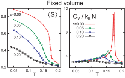
Figure 1: Average orientation amplitude $\langle{S}\rangle$ in Eq.(A4) (left) and specific heat $C_{V}$ in Eq.(3.1) divided by $k_{B}N$ (right) vs $T$ for $c=0.0,0.05,0.1$, and 0.2, which are calculated in the $NVT$ ensemble. The peak of $C_{V}$ decreases with increasing $c$.

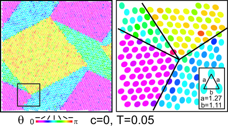
Figure 2: Left: Domain pattern composed of three martensitic variants for $c=0$ at $T=0.05$. Right: Elliptic particles around a junction of four domains in the box region in the left. The angles among the four lines are nearly equal to $\pi/2$ (for yellow square), $\pi/6$, $\pi/2$, and $5\pi/6$, being multiples of $\pi/6$. Each variant is composed of isosceles triangles with long side length $a=1.27\sigma_{1}$ and short one $b=1.11\sigma_{1}$ (inset). Colors represent $[\theta_{i}]_{\pi}$ according to the color bar.

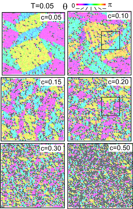
Figure 3: Frozen patterns of the angles $\theta_{i}$ of the ellipses at $T=0.05$ for $c=0.05,0.1$, 0.15, 0.2, 0.3, and 0.5. Colors of the ellipses represent $[\theta_{i}]_{\pi}$ according to the color bar, while black points ($\bullet$) represent impurities. With increasing impurity concentration $c$, the domains become smaller, resulting in orientational glass.

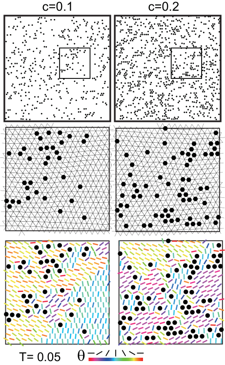
Figure 4: Top: Impurity distribution with significant clustering for $c=0.1$ (left) and 0.2 (right) at $T=0.05$. The data of these snapshots are common to those of $c=0.1$ and 0.2 in Fig.3. Middle: Delaunay diagrams in the box regions in the top panels (common to those in Fig.3), mostly composed of isosceles triangles. Impurities are also written $(\bullet)$. Bottom: Expanded snapshots of ellipses around impurities in the same regions, exhibiting planar anchoring with $[\theta_{i}]_{\pi}$ according to the color bar.

III NVT simulation of orientational glass on a hexagonal lattice

In Figs.1-4, we give results in the $NVT$ ensemble. Under Eqs.(2.11) and (2.13), the melting temperature $T_{m}$ was about $1.0$, above which liquid was realized. Below $T_{m}$, a hexagonal crystal without orientational order appeared. For $T\lesssim 0.4$, an orientational phase transition took place for small $c\lesssim 0.1$, while orientational glass emerged for not small $c\gtrsim 0.2$. Previously, many authors Frenkel1 examined the phase transition between orientationally disordered and ordered crystal phases for monodisperse hard rods with mild aspect ratios.

III.1 Order parameter amplitude and specific heat

In Fig.1, we plot the average orientation amplitude $\langle{S}\rangle$ defined in Appendix A and the constant-volume specific heat $C_{V}=(\partial{\langle{H}\rangle}/\partial{T})_{NV}$ vs $T$ for four concentrations. The former represents the overall strength of the orientational order, while the latter is the fluctuation amplitude of the energy $H$ in the $NVT$ ensemble,

$$C_{V}=\langle{(H-\langle{H}\rangle)^{2}}\rangle/k_{B}T^{2}.$$ (3.1)

Hereafter, $\langle{\cdots}\rangle$ denotes the average over time and over several runs. For $c=0$, $\langle{S}\rangle$ grows nearly discontinuously at $T=0.18$ in a narrow temperature window with width about $0.02$, where the disordered and ordered phases coexist. However, its $T$ dependence becomes gradual for $c>0$. The $C_{V}$ exhibits a peak at the orientational transition and its peak height decreases with increasing $c$. This peak stems from the enhanced orientation fluctuations near the transition.

In the same situation with the same $N$, we also performed simulation in the $NpT$ ensemble with an isotropic applied stress in two dimensions (not shown in this paper), where we allowed the cell to take a rectangular shape. There, the transition was first-order with discontinuous changes in volume and entropy comment1 as in three-dimensional KCN Mertz ; St ; Raedt ; Bell ; Kob-Binder . We also found a sharp peak in the isobaric specific heat $C_{p}$ at the transition. For $c\gtrsim 0.1$, the impurities pin the domain growth and the $NVT$ and $NpT$ simulations provide essentially the same low-$T$ behavior.

In previous experiments on (KCN)_1-c(KBr)_c, $C_{p}$ exhibited peaks as a function of $T$ at structural phase transitions for small $c$, but it varied continuously without peaks for large $c$ ori ; Mertz . In addition, the peak height for small $c$ was of order $5k_{B}$ per molecule. These features are common to those of our specific heat results.

III.2 Structural phase transition for $c=0$ and fragmentation of domains for $c>0$

In the one-component case $c=0$, the ellipses undergo a first-order structural (martensitic) phase transition from a hexagonal lattice to a deformed hexagonal lattice formed by isosceles triangles. The transition temperature is about 0.18 under Eq.(3.1) as indicated by Fig.1. In Fig.2, we show a typical orientational pattern of oriented domains for $c=0$ below the transition at fixed $V$. Depicted are the angles,

$$[\theta_{i}]_{\pi}=\theta_{i}-k\pi$$ (3.2)

in the range $[0,\pi]$ with $k$ being an integer, where $\theta_{i}$ and $\theta_{i}\pm\pi$ are not differentiated. There appear three crystalline variants with the same volume fraction $1/3$. Here, ${\mbox{\boldmath$n$}}_{i}$ are aligned along one of the underlying crystal axes, so each variant is composed of isosceles triangles elongated along its orientated direction. The domains are separated by sharp interfaces, where the surface tension is about $0.2$ in units of $\epsilon/\sigma_{1}^{2}$. As a unique feature, the junctions, at which domain boundaries intersect, have angles $\pi n/6$ ($n=1,2,\cdots)$ approximately. Similar unique domain patterns were experimentally observed on hexagonal planes after structural phase transitions Kitano . They were also reproduced in 2D phase-field simulations Chen ; Onukibook .

Next, it is of great interest how the domain structure is influenced by impurities. In Fig.3, we present snapshots of $[\theta_{i}]_{\pi}$ at $T=0.05$ for $c=0.05,0.1$, 0.15, 0.2, 0.3, and 0.5. At this low $T$, the thermal fluctuations are very small and the patterns of $[\theta_{i}]_{\pi}$ are nearly frozen in time even on a time scale of $10^{5}$, though flip rotations are still activated infrequently (see the bottom panels of Fig.5 below). We can see that the domains gradually become finely divided with increasing $c$. The fractions of the three variants are the same ($1/3)$ at fixed $V$. For $c\gtrsim 0.2$, the orientational disorder is much enhanced, resulting in orientational glass. We note that the distribution of $[\theta_{i}]_{\pi}$ is peaked at the three angles along the crystal directions (even for $c=0.5)$ (see Fig.15 below).

III.3 Impurity clustering and planar anchoring

The top panels of Fig.4 display the overall impurity distributions for $c=0.1$ and 0.2 at $T=0.05$. We can see a significant tendency of clustering of the impurities, which took place mostly during liquid states in the quenching process. In the present model, association of the impurities lowers the total potential energy by about $-5\epsilon$ per impurity EPL . In contrast, such impurity clustering has been neglected in spin glass theories Binder ; Kob-Binder .

In the middle plates of Fig.4, the Delaunay triangulation is given for the particle configurations in the box regions in the upper panels, which are the dual graphs of the Voronoi diagrams. They are mostly composed of isosceles triangles in the inset of Fig.2. With impurities of size ratio 1.2, the hexagonal lattice is locally elongated, but its structure is preserved, where the number of triangles surrounding each particle (the coordination number) $k$ is mostly 6. In Figs.3 and 4, there appear particles with $k=5$ and those with $k=7$. They are both two ellipses for $c=0.1$, while they are both seven (including two impurities with $k=7$) for $c=0.2$. See Fig.11(b) below for such defects.

In the bottom panels of Fig.4, we present expanded snapshots of anisotropic particles around impurities. The alignments are mostly perpendicular to the surface normals of the impurities, analogously to the planar anchoring of liquid crystal molecules near colloid surfaces PG . Domain boundaries between different variants can also be seen.

To examine the degree of clustering of the impurities, let us group them into clusters. We assume that two impurities $i$ and $j$ belong to the same cluster if their distance is shorter than $1.6$. Then, we calculate the numbers $N_{\rm I}(\ell)$ of the $\ell$ clusters consisting of $\ell$ impurities, where $\sum_{\ell\geq 1}\ell N_{\rm I}(\ell)=N_{2}$. The average cluster size is given by

$${\ell}_{\rm I}=\sum_{\ell}\ell^{2}N_{\rm I}(\ell)/N_{2}$$ (3.3)

In Fig.3, we have ${\ell}_{\rm I}=1.37$, 2.04, 3.02, 4.79, 10.7, and 984 for $c=0.05$, 0.1, 0.15, $0.2$, 0.3, and 0.5, respectively. For $c=0.5$, a cluster of the system size $\sim 1400$ appears.

IV NVE simulation of rotational dynamics

In Figs.5-12, we give simulation results in the $NVE$ ensemble, where the average translational and rotational kinetic energies were kept at $k_{B}T$ and $k_{B}T/2$, respectively, per particle. Varying $T$, we examine the rotational dynamics at $c=0.2$. For $0.3\lesssim T\lesssim 0.7$, we realize the rotator phase, where non-flip rotations with angle changes not close to $\pm\pi$ are gradually arrested with lowering $T$. For $T\lesssim 0.3$, quadrupolar glass is realized, where only flip rotations can be activated heterogeneously.

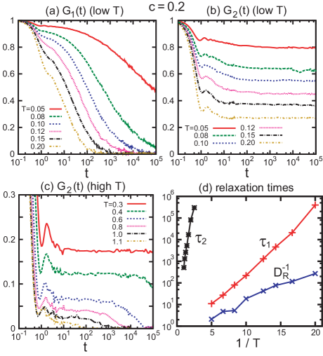
Figure 5: Orientational relaxations for $c=0.2$ at various $T$. (a) $G_{1}(t)$ and (b) $G_{2}(t)$ at low $T=$0.05,0.08,0.10,0.12, 0.15, and 0.20. (c) $G_{2}(t)$ at relatively high $T=$0.3,0.4,0.6,0.8, 1.0, and 1.1. (d) Relaxation times $\tau_{1}$ from $G_{1}(t)$ at low $T$ in Eq.(4.3), $\tau_{2}$ from $G_{2}(t)$ at high $T$ in Eq.(4.4), and the inverse rotational diffusion constant $D_{R}^{-1}$ in Eq.(4.12).

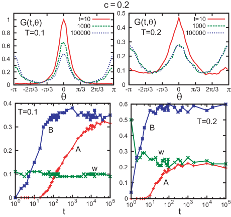
Figure 6: Top:Time-dependent angle distribution $G(t,\theta)$ in Eq.(4.5) for $c=0.2$ at $t=10,10^{3}$, and $10^{5}$. Here, $T=0.1$ and $\tau_{1}=220$ (left), while $T=02$ and $\tau_{1}=220$ (right). Bottom: Parameters $A$, $B$, and $w$ in the approximate expression (4.8) for $T=0.1$ and 0.2 as functions of $t$.

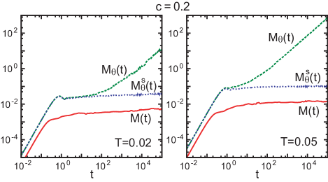
Figure 7: $M_{\theta}(t)$ in Eq.(4.11), $M(t)$ in Eq.(4.13), and $M_{\theta}^{s}(t)$ in Eq.(4.14) for $c=0.2$ at $T=0.02$ (left) and $T=0.05$ (right). These are the averages of $(\Delta\theta_{i})^{2}$, $|\Delta{\mbox{\boldmath$r$}}_{i}|^{2}$, and $\sin^{2}(\Delta\theta_{i})$, respectively. At these low $T$, $M(t)$ and $M_{\theta}^{s}(t)$ tend to plateaus, but $M_{\theta}(t)$ exhibits linear growth at long times due to flip rotations. Then, $D_{R}$ is $0.75\times 10^{-4}$ at $T=0.02$ and $3.5\times 10^{-3}$ at $T=0.05$. Transient plateau behavior can also be seen in $M_{\theta}(t)$ at $T=0.02$.

IV.1 Rotational time-correlation functions

The rotational dynamics has been extensively investigated for anisotropic particles in glassy states Kob1 ; Lewis ; EPL ; Schilling ; Sch . We consider the rotational time-correlation functions $G_{1}(t)$ and $G_{2}(t)$ for the ellipses defined by

$$G_{\ell}(t)=\frac{1}{N_{1}}\sum_{j\in 1}\bigg{\langle}{\cos[\ell\Delta\theta_{j}(t_{0},t_{0}+t)]}\bigg{\rangle},$$ (4.1)

where $\ell=1$, 2. We write the angle change of ellipse $i$ as

$$\Delta\theta_{i}(t_{0},t_{1})=\theta_{i}(t_{1})-\theta_{i}(t_{0}).$$ (4.2)

In 3D, use has been made of the Legendre polynomials $P_{\ell}(\theta)$. In Fig.5, we show $G_{1}(t)$ and $G_{2}(t)$ for $c=0.2$ at various temperatures. For low $T\leq 0.2$, the relaxation of $G_{1}(t)$ is slowed down with lowering $T$ in (a), while $G_{2}(t)$ tends to a plateau $f_{2}(T)$ for $t\gtrsim 10^{2}$ after considerable initial relaxations in (b). For higher $T\geq 0.4$, $G_{2}(t)$ decays at long times in (c). Relaxation times vs $1/T$ are plotted in (d), where $\tau_{1}$ of $G_{1}(t)$ is determined by

$$G_{1}(\tau_{1})=e^{-1}.$$ (4.3)

At long times, $G_{2}(t)$ relaxes only for $T\geq 0.4$ and its relaxation time $\tau_{2}$ is determined by its fitting to the stretched exponential form,

$$G_{2}(t)\cong f_{2}\exp[-(t/\tau_{2})^{\beta}].$$ (4.4)

In our case, we find $\beta\cong 1$. In the Arrhenius form, we obtain $\ln(\tau_{1})=0.68/T-1.2$ for $T\lesssim 0.2$ and $\ln(\tau_{2})=4.2/T+2.5$ for $T\gtrsim 0.4$. Note that these two temperature ranges are separated.

The difference between $G_{1}(t)$ and $G_{2}(t)$ can be understood if we consider the distribution of the angle changes,

$$G(t,\theta)=\frac{1}{N_{1}}\sum_{i\in 1}\bigg{\langle}{\delta([\Delta\theta_{i}(t_{0},t+t_{0})]_{2\pi}-\theta)}\bigg{\rangle},$$ (4.5)

where $-\pi\leq\theta<\pi$. For any $\Delta\theta_{i}$, we set

$$[\Delta\theta_{i}]_{2\pi}=\Delta\theta_{i}-2k\pi,$$ (4.6)

in the range $[-\pi,\pi]$ with an integer $k$. This $G(t,\theta)$ tends to $\delta(\theta)$ as $t\to 0$ and broadens gradually for $t>0$. The $G_{\ell}(t)$ in Eq.(4.1) can be written as

$$G_{\ell}(t)=\int_{-\pi}^{\pi}d\theta G(t,\theta)\cos(\ell\theta).$$ (4.7)

In the top panels of Fig.6, we plot time-evolution of $G(t,\theta)$ for $c=0.2$ at $T=0.1$ and 0.2. Salient features are as follows. (i) The width of the peak at $\theta=0$, written as $\sqrt{w}$, soon tends to be independent of $t$. For $t\gg 1$, $w$ represents the vibrational amplitude of the ellipses (see Eq.(4.10)). We obtain $w=0.09$, 0.17, and 0.22 at $T=0.1$, 0.15, and $0.2$, respectively. (ii) For $t\gtrsim\tau_{1}$, $G(t,\theta)$ exhibits secondary peaks at $\theta=\pm\pi$ due to the flip motions $\theta_{i}\to\theta_{i}\pm\pi$. Their peak widths are nearly equal to that of the main peak at $\theta=0$. (iii) The midpoint values $G(t,\pm\pi/2)$ become appreciable at long times.

We may thus approximate $G(t,\theta)$ as a superposition of a constant and Gaussian functions as

$$G(t,\theta)\cong\frac{B}{2\pi}+\frac{1-A-B}{\sqrt{2\pi w}}{e^{-{\theta^{2}}/{2w}}}$$

$$+\frac{A}{\sqrt{2\pi w}}\bigg{[}{e^{-{(\theta-\pi)^{2}}/{2w}}}+{e^{-{(\theta+\pi)^{2}}/{2w}}}\bigg{]}.$$ (4.8)

where $A$ is the turnover probability and $B/2\pi$ is the homogeneous part. We fit the calculated $G(t,\theta)$ to the above form to obtain $w(t)$, $A(t)$, and $B(t)$ vs $t$ for $T=0.1$ and 0.2 in the bottom panels of Fig.6. Here, $w(t)$ and $B(t)$ are nearly constant for $t\gg 1$, while $A(t)$ tends to saturate for $t\gtrsim 10^{5}$ at $T=0.1$ and for $t\gtrsim 10^{3}$ at $T=0.2$. Also $w$ remains so small such that the Gaussian functions in Eq.(4.8) are negligible at the midpoints $\theta=\pm\pi$ compared to $B/2\pi$. The plateau $f_{2}$ of $G_{2}(t)$ in Fig.5(b) is expressed as

$$f_{2}\cong(1-B)\exp({-2w}).$$ (4.9)

Substitution of the calculated values of $B$ and $w$ into the above expression yields $f_{2}=0.54$, 0.37, and 0.26 for $T=0.1$, 0.15, and 0.2, respectively, in excellent agreement with $f_{2}$ in Fig,5(b). On the other hand, at higher $T(\gtrsim 0.4)$, the system is in the plastic solid phase and $G(t,\theta)$ tends to be homogeneous ($=1/2\pi$) very slowly for $t\gg\tau_{2}$, leading to the long-time decay of $G_{2}(t)$ in Fig.5(c).

We comment on the meaning of $w$ in Eq.(4.8). Let $\bar{\theta}_{i}$ be the time average of $\theta_{i}$ over many vibrations, where we neglect flip rotations. Then, we have $\Delta{\theta}_{i}(t_{0},t_{1})=\delta\theta_{i}(t_{1})-\delta\theta_{i}(t_{0})$ in Eq.(4.2), where $\delta{\theta}_{i}={\theta}_{i}-\bar{\theta}_{i}$ is the deviation from the equilibrium angle $\bar{\theta}_{i}$. With increasing $t=t_{1}-t_{0}$, $\delta\theta_{i}(t_{1})$ and $\delta\theta_{i}(t_{0})$ should become uncorrelated to give $\sum_{i}\delta\theta_{i}(t_{1})\delta\theta_{i}(t_{0})/N_{1}=0$ so that

$$w=2\langle{\delta\theta^{2}}\rangle=2\sum_{i\in 1}|\delta\theta_{i}|^{2}/N_{1},$$ (4.10)

where $\langle{\delta\theta^{2}}\rangle$ is the variance of $\delta\theta_{i}$ over all the ellipses.

IV.2 Angular mean-square displacement

In the literature Kob1 ; Lewis , the rotational diffusion has been discussed in terms of the angular mean-square displacement of the ellipses,

$$M_{\theta}(t)=\langle{(\Delta\theta)^{2}}\rangle=\frac{1}{N_{1}}\sum_{i\in 1}\langle{[\Delta\theta_{i}(t_{0},t_{0}+t)]^{2}}\rangle.$$ (4.11)

which exhibits the ballistic behavior $(\propto t^{2})$ for $t\lesssim 1$ and the diffusion behavior for $t\gg 1$ as

$$M_{\theta}(t)\cong 2D_{R}t.$$ (4.12)

See Fig.5(d), where $\ln(D_{R}^{-1})=0.33/T-0.68$ in the Arrhenius form. These behaviors are analogous to those of the positional mean-square displacement,

$$M(t)=\langle{|\Delta{\mbox{\boldmath$r$}}|^{2}}\rangle=\frac{1}{N_{1}}\sum_{i\in 1}\langle{|\Delta{\mbox{\boldmath$r$}}_{i}(t_{0},t_{0}+t)|^{2}}\rangle.$$ (4.13)

where $\Delta{\mbox{\boldmath$r$}}_{i}(t_{0},t_{0}+t)={\mbox{\boldmath$r$}}_{i}(t_{0}+t)-{\mbox{\boldmath$r$}}_{i}(t_{0})$ is the displacement vector of ellipse $i$ in time interval $[t_{0},t_{0}+t]$. In Fig.7, we plot $M_{\theta}(t)$ and $M(t)$ vs $t$ at low $T=0.02$ and 0.05 for $c=0.2$. Here, $M(t)$ saturates at a plateau, but $M_{\theta}(t)$ still exhibits the diffusion behavior. As Fig.6 suggests, this difference originates from flip rotations without positional changes. To confirm this, we also plot the mean-square displacement of $\sin(\Delta\theta_{i})$ written as

$$M_{\theta}^{s}(t)=\frac{1}{N_{1}}\sum_{i\in 1}|\sin[\Delta\theta_{i}(t_{0},t_{0}+t)]|^{2}/N_{1},$$ (4.14)

which is insensitive to flip rotations. As ought to be the case, $M_{\theta}^{s}(t)$ coincides with $M_{\theta}(t)$ at short times but tends to a plateau at long times. We also notice that $M_{\theta}(t)$ exhibits a plateau in the range $1\lesssim t\lesssim 100$ at $T=0.02$.

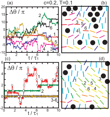
Figure 8: Time-evolution of angle changes $\Delta\theta_{i}(t_{0},t_{0}+t)$ in Eq.(4.1) (left) for $c=0.2$ and $T=0.1$, where $\tau_{1}=220$. Selected ellipses are numbered $1,\cdots,6$ and impurities are written as large circles ($\bullet$) (right). (a) Rotationally active ellipses not anchored by impurities. Ellipse 2 is active though it is rather close to impurities. (c) Inactive ones in an orientationally ordered domain ($3-6$) and relatively active ones in an interfacial region ($1$ and $2$). On the curve of ellipse 1, the flip times are marked ($\circ$) (see the Appendix B).

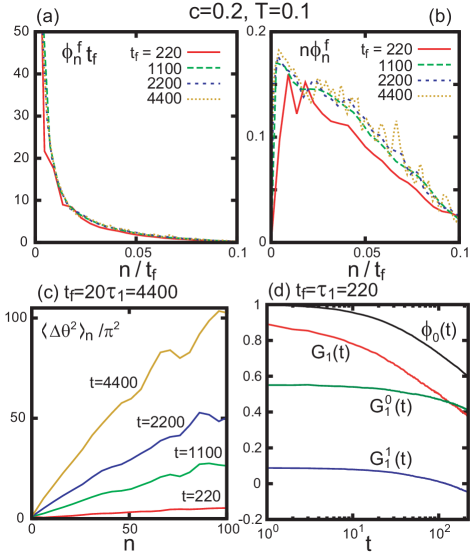
Figure 9: (a) $t_{f}\phi_{n}^{f}$ and (b) $n\phi_{n}^{f}$ vs $n/t_{f}$ for $t_{f}/\tau_{1}=1,5,10,$ and 20 with $\tau_{1}=220$. (c) $\langle{\Delta\theta^{2}}\rangle_{n}(t)/\pi^{2}$ vs $n$ at $t/\tau_{1}=1,5,10$, and 20. Here, $c=0.2$ and $T=0.1$. See Eqs.(4.15) and (4.18) for $\phi_{n}^{f}$ and $\langle{\Delta\theta^{2}}\rangle_{n}(t)$. (d) $G_{1}(t)$ in Eq.(4.1), $G_{1}^{n}(t)$ ($n=0,1$) with $t_{f}=\tau_{1}$ in Eq.(4.23), and $\phi_{0}(t)$ in Eq.(4.24).

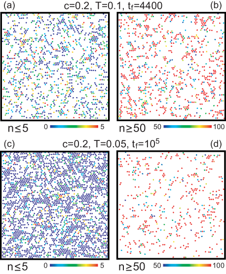
Figure 10: Top: Snapshots of ellipses at $T=0.1$ with $n_{i}\leq 5$ in (a) and with $n_{i}\geq 50$ in (b). Bottom: Snapshots of ellipses at $T=0.05$ with $n_{i}\leq 5$ in (c) and with $n_{i}\geq 50$ in (d). Depicted ellipse fractions are (a) 0.36, (b) 0.27, (c) 0.72, and (d) 0.15. These rotationally inactive and active ellipses exhibit heterogeneities closely correlated with the impurity clustering (see the top right panel in Fig.4).

IV.3 Flip rotations in orientational glass

The rotational activity of the anisotropic particles sensitively depends on the surrounding particle configurations. In Fig.8, we show typical time-evolution of the angle changes. Rotationally inactive ellipses are those anchored to impurities and those within orientationally ordered domains, while rotationally active ones are those in disordered regions not anchored to impurities and those in interfacial regions between different domains.

As will be shown in Appendix B, we may numerically determine flip events. That is, within any time interval $[t_{0},t_{0}+t_{f}]$, each ellipse $i$ flips at successive times $t_{0}+t_{i1},t_{0}+t_{i2},\cdots,t_{0}+t_{in_{i}}$ with $t_{i1}>0$ and $t_{in_{i}}<t_{f}$, where $n_{i}$ is the flip number of ellipse $i$. The fraction of the ellipses with $n$ flips is expressed as

$$\phi_{n}^{f}=\langle{\sum_{i\in 1}\delta_{nn_{i}}}\rangle/N_{1},$$ (4.15)

where $\sum_{n}\phi_{n}^{f}=1$. We do not write the $t_{f}$-dependence of $n_{i}$ and $\phi_{n}^{f}$ explicitly. We divide the ellipses into groups ${\cal F}_{0}$, ${\cal F}_{1}$, $\cdots,{\cal F}_{n_{\rm max}}$, where those in ${\cal F}_{n}$ have undergone $n$ flips in the time interval $[t_{0},t_{0}+t_{f}]$. We introduce the maximum flip number $n_{\rm max}$ among all the ellipses. For large $n$ and $t_{f}$, we should have the scaling relation,

$$\phi_{n}^{f}=\Phi_{f}(n/t_{f})/t_{f},$$ (4.16)

where $\Phi_{f}(x)$ is a scaling function. In particular, $n_{\rm max}$ is proportional to $t_{f}$ as

$$n_{\rm max}=A_{\rm max}t_{f}.$$ (4.17)

The coefficient $A_{\rm max}$ is about $0.11$ at $T=0.1$ and $0.022$ at $T=0.05$.

We then introduce the angular mean-square displacement within the group ${\cal F}_{n}$ as

$$\langle{\Delta\theta^{2}}\rangle_{n}(t)=\frac{1}{N_{1}\phi_{n}^{f}}\bigg{\langle}{\sum_{i\in{\cal F}_{n}}[\Delta\theta_{i}(t_{0},t_{0}+t)]^{2}}\bigg{\rangle}.$$ (4.18)

which is a function of $t$ for each given $t_{f}$. The total angular mean square displacement is expressed as

$$M_{\theta}(t)=\sum_{1\leq n\leq n_{\rm max}}\phi_{n}^{f}\langle{|\Delta\theta|^{2}}\rangle_{n}(t).$$ (4.19)

For sufficiently large $t$ and $n$, the ellipses in the group ${\cal F}_{n}$ should have undergone $nt/t_{f}$ flips on the average. Then, in the diffusion regime, we should have

$$\langle{\Delta\theta^{2}}\rangle_{n}\cong\pi^{2}nt/t_{f}.$$ (4.20)

Here, the angle changes $\Delta\theta_{i}(t_{0},t_{0}+t)$ at jumps are $\pi$ or $-\pi$ and their distribution should be nearly Gaussian.

In Fig.9, we show numerical results which are the averages over six runs. We plot $t_{f}\phi_{n}^{f}=\Phi_{f}(x)$ in (a) and $n\phi_{n}^{f}=x\Phi_{f}(x)$ in (b) as functions of $x=n/t_{f}$ ($n\geq 1$) for $c=0.2$ and $T=0.1$ by setting $t_{f}/\tau_{1}=1,5,10,$ and 20 ($\tau_{1}=220)$. These curves are nearly independent of $t_{f}$, which confirms the scaling form (4.16). However, the ellipses without flips still remain, whose fraction is $\phi_{0}^{f}=0.17$ even for $t_{f}=20\tau_{1}$. From Fig.9(b), for large $n$, $\phi_{n}^{f}$ may be fitted to

$$\phi_{n}^{f}\cong A_{f}\bigg{(}\frac{1}{n}-\frac{1}{n_{\rm max}}\bigg{)},$$ (4.21)

where $A_{f}\cong 0.20$ and $n_{\rm max}\cong 500$ at $T=0.1$. The $A_{f}$ is independent of $t_{f}$. In (c), we also confirm Eq.(4.20). From Eqs.(4.12), (4.17), and (4.19)-(4.21), we obtain

$$D_{R}\cong\frac{1}{4}\pi^{2}A_{f}A_{\rm max},$$ (4.22)

which yields $D_{R}\sim 0.056\sim 13/\tau_{1}$ at $T=0.1$ in good agreement with the result from the slope of $M_{\theta}(t)$. At $T=0.05$, we again find Eq.(4.21) with $A_{f}\cong 0.048$, $n_{\rm max}\cong 2800$, and $\phi_{0}^{f}\cong 0.58$ for $t_{f}=10^{5}$. From Eq.(4.22) these lead to $D_{R}=0.0033\sim 1500/\tau_{1}$, while the right panel of Fig.7 yields $D_{R}=0.0035$. The rotational diffusion constant $D_{R}$ is thus determined by the rotationally active ellipses with $n_{i}\sim n_{\rm max}$.

In contrast, the main contribution to $G_{1}(t)$ in Eq.(4.1) is from the ellipses which have undergone no flip in time interval $[t_{0},t_{0}+t]$. This is the reason why $\tau_{1}$ behaves very differently from $D_{R}^{-1}$ in Fig.5(d). To show this, we set $t_{f}=\tau_{1}$. We then consider the following partial sums,

$$G_{1}^{n}(t)=\frac{1}{N_{1}}\bigg{\langle}{\sum_{i\in 1,n_{i}=n}\cos[\Delta\theta_{i}(t_{0},t_{0}+t)]}\bigg{\rangle}.$$ (4.23)

In Fig.9(d), we compare $G_{1}^{0}(t)$ (no-flip contribution) and $G_{1}^{1}(t)$ (single-flip contribution) with $G_{1}(t)$. Here, $G_{1}^{0}(\tau_{1})=0.41=1.11/e$ and $G_{1}^{1}(\tau_{1})=-0.05$, so $G_{1}(\tau_{1})=1/e$ mostly consists of the no-flip contribution. We also display the fraction of the ellipses with no flip in time interval $[t_{0},t_{0}+t]$, denoted by $\phi_{0}(t)$. Treating $\phi_{0}^{f}$ in Eq.(4.15) as a function of $t_{f}$, we have

$$\phi_{0}(t)=[\phi_{0}^{f}]_{t_{f}=t}.$$ (4.24)

In Fig.9(d), we find $\phi_{0}(\tau_{1})=0.60$. If $\phi_{0}(t)$ is shifted by 0.1 downward, it nearly coincides with $G_{1}(t)$.

In Figs.10, we show snapshots of the ellipses with $n\leq 5$ (left) and $n\geq 50$ (right) for $T=0.1$ and $t_{f}=4400$ (top) and for 0.05 and $t_{f}=10^{5}$ (bottom). The distributions of these rotationally inactive and active ellipses are highly heterogeneous. This marked feature is due to the significant impurity clustering in the top right panel in Fig.4. With lowering $T$, the flip rotations become increasingly infrequent. In fact, the fraction of the ellipses with $n\geq 50$ are 0.36, 0.15, and 0.005 for $(T,t_{f})=(0.1,4400)$, $(0.05,10^{5})$, and $(0.02,10^{5})$, respectively.

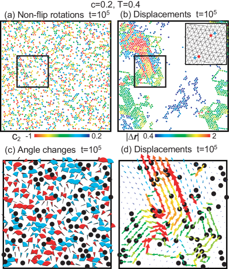
Figure 11: Non-flip rotations and displacements between two times $t_{0}$ and $t_{0}+t$ with $t=10^{5}$ for $c=0.2$ and $T=0.4$, where orientational glass is approached from plastic solid. Top: (a) Particles with $c_{2i}=\cos[2\Delta\theta_{i}]<0.2$ forming clusters and (b) those with large displacements $\Delta{r}_{i}>0.4$ caused by defect motions. Depicted particle numbers are $0.5N_{1}$ in (a) and $0.35N$ in (b). Colors represent $c_{2i}$ and $\Delta{r}_{i}$ according to the color bars. Expanded snapshot of a defect is also given (inset). (c) Expanded snapshot of the ellipses in the box region in (a), where each ellipse $i$ is written as an circular sector with two arcs parallel to ${\mbox{\boldmath$n$}}_{i}(t_{0})$ and ${\mbox{\boldmath$n$}}_{i}(t_{0}+t)$. They are written in blue for clockwise rotation ($\Delta\theta_{i}<0$) and in red for counterclockwise rotation ($\Delta\theta_{i}>0$). Impurities are also depicted($\bullet$). (d) Expanded snapshot of the particles with large displacements in the box region in (b), where red (green) arrows represent displacements by two (one) lattice constants.

IV.4 Non-flip rotations in plastic solids at relatively high temperature

So far we have studied the rotational dynamics in orientational glass. We should also examine the crossover from plastic solid to orientational glass at higher $T$. In this high $T$-regime, the long-time decay of $G_{2}(t)$ first saturates at the plateau in Eq.(4.9) and slowly decays to zero on the time scale of $\tau_{2}$ as in Fig.5(c). Some ellipses are attached to impurities on very long time scales and the homogenization of $G(t,\theta)$ takes a very long time.

In Fig.11, we hence display large non-flip rotations and long-distance displacements between two times $t_{0}$ and $t_{0}+t$ with $t=10^{5}$ for $c=0.2$ and $T=0.4$. Here, the particle positions depicted are those ${\mbox{\boldmath$r$}}_{i}(t_{0})$ at the initial time $t_{0}$. The flip numbers of the ellipses in this time interval are huge, ranging from $10^{3}$ to $10^{4}$. In (a), we pick up the ellipses with $c_{2i}(t)<0.2$, where we define

$$c_{2i}(t)=\cos[2\Delta{\theta}_{i}(t_{0},t_{0}+t)].$$ (4.25)

Because $c_{2i}$ is invariant with respect to turnovers ${\theta}_{i}\to{\theta}_{i}\pm\pi$, it deviates from unity significantly due to non-flip rotations. The condition $c_{2i}(t)<0.2$ means $0.22\pi<[\Delta{\theta}_{i}(t_{0},t_{0}+t)]_{\pi}<0.78\pi$ in terms of $[\Delta\theta_{i}]_{\pi}$ in Eq.(3.2). In (b), we mark the particles with $\Delta{r}_{i}(t)=|{\mbox{\boldmath$r$}}_{i}(t_{0}+t)-{\mbox{\boldmath$r$}}_{i}(t_{0})|>0.4$. These displacements are induced by intermittent motions of a few pointlike defects. As in the inset of Fig.11(b), they are composed of two particles with their coordination numbers equal to five and seven (see the explanation of the middle panels if Fig.4 also). These defects have been observed in a number of simulations and experiments in two dimensions defects . The lengths of the large displacements are then mostly $a$ or $2a$ with $a$ being the lattice constant, so they do not affect the hexagonal crystal structure. In (c), an expanded snapshot of the box region in (a) is presented, where each ellipse $i$ is written as an circular sector with two arcs parallel to ${\mbox{\boldmath$n$}}_{i}(t_{0})$ and ${\mbox{\boldmath$n$}}_{i}(t_{0}+t)$. In (d), an expanded snapshot of the box region in (b) is presented with displacement vectors in arrows.

In Fig.11(a), we can see marked clustering of many ellipses with significant non-flip rotations, which is strongly correlated with the heterogeneous impurity distribution. In Fig.11(c), we further notice the presence of considerable thermal motions superimposed. Also in regions without defects (in the upper middle part from Fig.11(b)), we may also write expanded figures, but they are similar to Fig.11(c). Let $N_{\rm cl}(\ell)$ be the numbers of the $\ell$ clusters consisting of $\ell$ ellipses with $c_{2i}<0.2$, where two ellipses $i$ and $j$ belong to the same cluster for $r_{ij}<1.6$. As in Eq.(3.3), the average cluster size may be defined as

$${\ell}_{\rm cl}=\sum_{\ell}\ell^{2}N_{\rm im}(\ell)/N_{1}.$$ (4.26)

Then we find ${\ell}_{\rm cl}=48$ for the snapshot in Fig.11(a).

V Rheology in orientational glass

In Figs.12-15, we imposed a Parrinello-Rahman barostat Rahman together with a Nos$\acute{\rm e}$-Hoover thermostat nose under the periodic boundary condition. In our system, small crystalline domains are elongated along the orientations of the ellipses and their orientation changes can give rise to a macroscopic strain. We here predict a shape memory effect in orientational glass, where soft elasticity appears without dislocation formation. See Ref.EPL for preliminary results of 3D simulation on rheology.

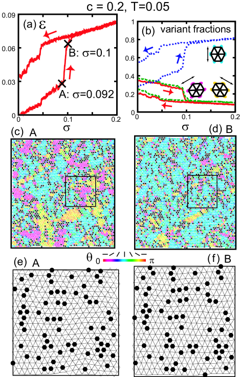
Figure 12: Shape memory effect under stretching for $c=0.2$ and $T=0.05$. (a) Strain $\varepsilon$ vs applied stress ${\sigma}$. Between points A ($\sigma=0.092$) and B ($\sigma=0.10$), the variant elongated along the $y$ axis increases yielding soft elasticity. The favored variant remains dominant on the return path. (b) Fractions of the three variants during the cycle, which are elongated along the three crystal axes. In (c) and (d), $[\theta_{i}]_{\pi}$ are written at points A and B in (a). In e) and (f), Delaunay diagrams of the box regions in (c) and (d) are given.

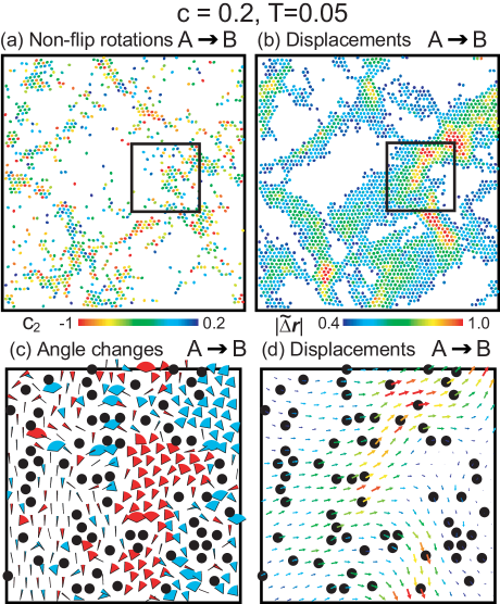
Figure 13: (a) Ellipses with large non-flip rotation $c_{2i}<0.2$ and (b) particles with large non-affine displacement $|\tilde{\Delta}{\mbox{\boldmath$r$}}_{i}|>0.4$ between two points A and B in Fig.12, where soft elasticity is realized. Colors are given according to the color bars. (c) Expanded snapshot of the ellipses in the box region in (a), where each ellipse $i$ is written as an circular sector with two arcs parallel to ${\mbox{\boldmath$n$}}_{i}(t_{0})$ and ${\mbox{\boldmath$n$}}_{i}(t_{0}+t)$ written in blue for clockwise rotation and in red for counterclockwise rotation. (d) Expanded snapshot of the particles with large non-affine displacement in the box region in (b).

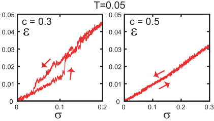
Figure 14: Stress-strain curve for $c=0.3$ (left) and 0.5 (right). For $c=0.3$ the loop is closed at positive $\sigma$ and there remains no remnant strain (superelasticity). For $c=0.5$ there is no hysteresis and curve is linear in the range $0\leq\sigma\leq 0.3$.

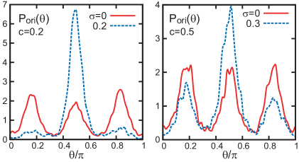
Figure 15: Orientational distribution $P_{\rm ori}(\theta)$ in Eq.(5.9) for $c=0.2$ (left) and 0.5 (right) for the initial point $\sigma=0$ and the point with maximum $\sigma$ ($0.2$ or 0.3) in the stress cycle. It has three peaks with equal heights for $\sigma=0$ and the peak at $\theta\cong\pi/2$ is increased at the maximum $\sigma$.

V.1 Shape memory effect

We stretched the system along the $y$ axis keeping the cell shape rectangular under the isothermal condition at $T=0.05$. We mention similar simulations in Refs.Falk ; Suzuki . In the following figures, the $x$ and $y$ axes are in the horizontal and vertical directions, respectively. One crystal axis of the crystal was made parallel to the $x$ axis. We controlled the space average of the $yy$ component of the stress. Its value is written as

$$\sigma=\langle{\sigma_{yy}}\rangle_{\rm s},$$ (5.1)

where $\langle{\cdots}\rangle_{\rm s}$ denotes the space average. The system was assumed to be stress-free along the $x$ axis. Thus,

$$\langle{\sigma_{xx}}\rangle_{\rm s}=0,$$ (5.2)

which is possible owing to the attractive part of the potential Falk . From the symmetry of the geometry, we also have $\langle{\sigma_{xy}}\rangle_{\rm s}=0$.

We started from a stress-free state with $\sigma=0$ in a square cell with length $L_{0}$. With applied stress, the cell lengths along the $x$ and $y$ axes are changed to $L_{x}$ and $L_{y}$. The average strain along the $y$ axis is written as

$$\varepsilon=L_{y}/L_{0}-1.$$ (5.3)

The effective Young modulus is defined by

$${E_{e}}=({d\varepsilon}/{d\sigma})_{T}^{-1}.$$ (5.4)

This means that an incremental change $\delta\sigma$ in the applied stress gives rise to an incremental strain $\delta\varepsilon=E_{e}^{-1}\delta\sigma$. Though $E_{e}$ nonlinearly depends on $\sigma$ in our case, we may also define the effective shear modulus $\mu_{e}$ using the linear elasticity relation $E_{e}=4K\mu_{e}/(K+\mu_{e})$, where $K$ is the bulk modulus related to the volume $V$ by $2\sigma/K=V/L_{y0}^{2}-1$. In our system, $K\gg E_{e}/4$ holds so that

$$\mu_{e}=E_{e}/(4-E_{e}/K)\cong E_{e}/4.$$ (5.5)

Hereafter, we measure $\sigma$ and $E_{e}$ in units of $\epsilon/\sigma_{1}^{2}$.

In Fig.12(a), we increased $\sigma$ slowly as $d\sigma/dt=4\times 10^{-6}$ from 0 up to 0.2 and then decreased $\sigma$ back to 0 as $d\sigma/dt=-4\times 10^{-6}$. The stretching pass is divided into four parts: (1) $0<\sigma<0.04$, (2) $0,04<\sigma<0.09$, (3) $0.09<\sigma<0.12$, and (4) $0.12<\sigma<0.20$, while the return path is divided into two parts: (5) $0.20>\sigma>0.05$, and (6) $0.05>\sigma>0$. The effective Young modulus $E_{e}$ is very small in the range (3). In fact, we have $E_{e}\cong 0.25$ between two points A ($\sigma=0.092$) and B ($\sigma=0.10$) in Fig.12(a), while $E_{e}\cong 4$ in the range (1) and $E_{e}\cong 8$ in the ranges (4) and (5). In addition, there appears a remnant strain ($\sim 0.03$) at the final point $\sigma=0$. Furthermore, if $T$ was raised above 0.2 in this final state, an orientationally disordered state was realized and a square shape of the cell was restored.

In Fig.12(b), we show the volume fractions of the three variants. See the sentences below Eq.(5.9) as to how they can be determined. We can see that the favored domains elongated along the $y$ axis increase and the disfavored ones decrease upon stretching. However, the favored domains do not much decrease in the return path, giving rise to the remnant strain. We also show the snapshot of the orientations at point A in (c) and that at point B in (d), between which the fractions of the favored variant are considerably different. In this stress cycle, a history-dependent loop is realized, where the impurities pin the orientation domains in quasi-stationary states under very slow variations of $\sigma$. In (e) and (f), we give Delaunay diagrams of the box regions in (c) and (d), where local strain variations can be seen without defects.

In Fig.13, we show the orientational and positional changes between two points A and B in Fig.12, which exhibit conspicuous large-scale heterogeneities. Displayed are (a) ellipses with large non-flip rotations with

$$c_{2i}(A,B)=\cos[2\theta_{i}(A)-2\theta_{i}(B)]<0.2$$ (5.6)

and (b) particles with large non-affine displacement

$$|\tilde{\Delta}{\mbox{\boldmath$r$}}_{i}(A,B)|>0.4.$$ (5.7)

Here, we write the angles and positions at A as $\theta_{i}(A)$ and ${\mbox{\boldmath$r$}}_{i}(A)=({x}_{i}(A),{y}_{i}(A))$ and those at B as $\theta_{i}(B)$ and ${\mbox{\boldmath$r$}}_{i}(B)=({x}_{i}(B),{y}_{i}(B))$. The $x$ and $y$ components of $\tilde{\Delta}{\mbox{\boldmath$r$}}_{i}(A,B)$ are defined by

$$\tilde{\Delta}{x}_{i}(A,B)={x}_{i}(B)-x_{i}(A)L_{x}(B)/L_{x}(A),$$

$$\tilde{\Delta}{y}_{i}(A,B)={y}_{i}(B)-y_{i}(A)L_{y}(B)/L_{y}(A),$$ (5.8)

where $L_{\mu}(A)$ and $L_{\mu}(B)$ are the cell lengths at A and B ($\mu=x,y$). For affine deformations, $\tilde{\Delta}{\mbox{\boldmath$r$}}_{i}(A,B)$ vanishes.

As in Fig.11(c), Fig.13(c) displays the ellipses in the box region in (a) written as circular sectors, whose arcs are parallel to ${\mbox{\boldmath$n$}}_{i}(A)$ and ${\mbox{\boldmath$n$}}_{i}(B)$ (in blue for $\theta_{i}(A)<\theta_{i}(B)$ and in red for $\theta_{i}(A)>\theta_{i}(B)$). The rotations are more collective with weaker thermal fluctuations than in Fig.11(c). In (d), the particles with large non-affine displacement (5.8) are written as arrows, which also indicates collective motions upon stretching. In both (c) and (d), the heterogeneities are strongly correlated with the inhomogeneous impurity distribution. The simulation time between A and B is 2000, so the flip numbers $n_{i}(A,B)$ between A and B are small. In fact, the ellipse number without flips $n_{i}(A,B)=0$ is $0.75N_{1}$, while that with $n_{i}(A,B)\geq 5$ is $0.04N_{1}$ with $n_{\rm max}(A,B)=10$.

We also find that the shape memory effect becomes weaker with increasing $c$, where the domain size is decreased. In Fig.14, the hysteresis loop diminishes for $c=0.3$ and vanishes for $c=0.5$. We recognize that mesoscopic orientational order is responsible for the singular mechanical response. However, a unique feature arises for $c=0.3$, though the loop is smaller. That is, the loop is closed at $\sigma\sim 0.03$ on the return path and the initial and final points coincide, resulting in no remnant strain at $\sigma=0$. It is worth noting that this stress-strain behavior, called superelasticity, has been observed in metallic alloys as a stress-induced martensitic phase transition marten ; Ren ; RenReview . In TiNi, this superelasticity effect appears at higher temperatures than the shape memory effect. For a model alloy system, Ding et al. Suzuki numerically studied the superelasticity effect.

Furthermore, in Fig.15, we plot the angle distribution,

$$P_{\rm ori}(\theta)=\sum_{i\in 1}\delta([\theta_{i}]_{\pi}-\theta)/N_{1},$$ (5.9)

at $T=0.05$. Each curve was results of a single run. This distribution has three peaks both for $c=0.2$ and $0.5$ in the directions of the three crystal axes and the peak at $\theta\cong\pi/2$ increases after stretching. This behavior is consistent with Fig.12(b). Here, we divide the ellipses into the three groups with $n/3\leq[\theta_{i}]_{\pi}/\pi<(n+1)/3$ ($n=0,1,2$) and calculate their volume fractions during stretching.

Table 1: Stress change $\Delta\sigma$, strain change $\Delta\varepsilon$, Young modulus $E_{e}$, change of fraction of the favored variant $\Delta\phi_{\rm va}$, fraction of orientational strain change $\gamma_{\rm ori}$, and ratio ${E_{e}}/\gamma_{\rm el}$ for $c=0.2$ and $T=0.05$, which are calculated between two points on the stress-strain curves. The last quantity should be equal to $E_{0}$ from Eq.(5.12).

$c$	$\sigma$	$\Delta\sigma$	$\Delta\varepsilon$	$E_{e}$	$\Delta\phi_{\rm va}$	$\gamma_{\rm ori}$	${E_{e}}/\gamma_{\rm el}$
0.2	0 $\to$ 0.04	0.04	0.010	4	0.05	0.75	16
0.2	0.092 $\to$ 0.1	0.008	0.032	0.25	0.21	0.98	15
0.2	0.12 $\to$ 0.2	0.08	0.011	8	0.04	0.55	18
0.3	0 $\to$ 0.1	0.1	0.014	7	0.06	0.64	18
0.3	0.11 $\to$ 0.12	0.11	0.010	1	0.06	0.94	18
0.3	0.12 $\to$ 0.2	0.08	0.018	4	0.09	0.72	16
0.5	0 $\to$ 0.15	0.15	0.014	11	0.04	0.43	19
0.5	0.15 $\to$ 0.3	0.15	0.018	8	0.07	0.56	18

V.2 Orientational strain

On the stress-strain curve, we consider two points between which the curve is nearly linear. See Figs.12 and 13 for examples. From Eq.(5.4) the stress change $\Delta\sigma$ and the strain change $\Delta\varepsilon$ are related by

$$\Delta\varepsilon=E_{e}^{-1}\Delta\sigma,$$ (5.10)

in terms of the effective Young modulus $E_{e}$. Generally, in the presence of a (proper) coupling between strain and orientation, $\Delta\varepsilon$ consists of three parts as

$$\Delta\varepsilon=\Delta\varepsilon_{\rm el}+\Delta\varepsilon_{\rm pl}+\Delta\varepsilon_{\rm ori},$$ (5.11)

First, the elastic part $\Delta\varepsilon_{\rm el}$ is approximately related to $\Delta\sigma$ by the linear elasticity relation,

$$\Delta\varepsilon_{\rm el}=E_{0}^{-1}\Delta\sigma,$$ (5.12)

where $E_{0}$ is the (bare) Young modulus in a single variant state being of order 20 in our case. Second, the plastic part $\Delta\varepsilon_{\rm pl}$ is due to plastic deformations. In the present example, there is no defect generation up to a large applied stress $\sigma_{\rm y}$, where $\sigma_{\rm y}\sim 0.5$ for $c=0.2$. Thus, we set $\Delta\varepsilon_{\rm pl}=0$ in this paper. Third, the orientational part $\Delta\varepsilon_{\rm ori}$ is related to the change of the volume fraction of the favored variant $\Delta\phi_{\rm va}$ as

$$\Delta\varepsilon_{\rm ori}=A_{0}\Delta\phi_{\rm va}.$$ (5.13)

where we calculate $\Delta\phi_{\rm va}$ from the angle distribution $P_{\rm ori}(\theta)$ in Eq.(5.9) (see Fig.15). We may determine the coefficient $A_{0}$ if we apply the relation (5.13) between the initial point $(\sigma,\varepsilon)=(0,0)$ and the final point $(\sigma,\varepsilon)=(0,0.03)$ on the stress-strain loop in Fig.12(a). Using $\Delta\phi_{\rm va}=0.2$ between these two points, we find $A_{0}=0.15$ for $c=0.2$.

It is convenient to define the ratios,

$$\gamma_{\rm el}=\Delta\varepsilon_{\rm el}/\Delta\varepsilon,\quad\gamma_{\rm ori}=\Delta\varepsilon_{\rm ori}/\Delta\varepsilon,$$ (5.14)

In this paper, we have $\gamma_{\rm el}+\gamma_{\rm ori}=1$ from $\Delta\varepsilon_{\rm pl}=0$. From Eq.(5.10) we obtain

$$E_{e}=E_{0}(1-\gamma_{\rm ori})=E_{0}\gamma_{\rm el}.$$ (5.15)

In Table 1, we give examples of the quantities, $\Delta\sigma$, $\Delta\varepsilon$, $E_{e}$, $\Delta\phi_{\rm va}$, $\gamma_{\rm ori}$, and ${E_{e}}/\gamma_{\rm el}$ for $c=0.2$, 0.3, and 0.5 at $T=0.05$. We set $A_{0}=0.15$ for these three concentrations, though it has been obtained for $c=0.2$. From Eq.(5.13) the last quantity ${E_{e}}/\gamma_{\rm el}$ should be equal to $E_{0}$ and is indeed calculated to be around 18.

VI Summary and remarks

We have presented an angle-dependent Lennard-Jones potential for binary mixtures in Eqs.(2.3) and (2.5) and performed MD simulation in two dimensions varying the concentration $c$ and the temperature $T$. In this paper, the aspect ratio is 1.2 and the size ratio is 1.2, so the crystal order is realized in all the examples treated. Our main results are as follows.
(i) In Sec.II, we have presented our model potential, which has the quadrupolar symmetry and is characterized by the anisotropy strength of repulsion $\chi$ in Eq.(2.5).
(ii)In Sec.III, we have presented results of $NVT$ simulation. First, the orientation amplitude $\langle{S}\rangle$ and the constant-volume specific heat $C_{V}$ have been presented as functions of $T$ around the orientational transition in Fig.1. Second, frozen orientational configurations at $T=0.05$ have been displayed for $c=0$ in Fig.2 and for six concentrations in Fig.3. These snapshots indicate how the domains are fragmented with increasing $c$ from martensitic multi-domain states to quadrupolar glassy states. In our system, the circular impurities exhibit significant clustering and anchor the ellipses around them in the planar alignment, as illustrated in Fig.4.
(iii) In Sec.IV, we have studied the rotational dynamics of the ellipses, where the orientation relaxations are two-fold. In Fig.5, $G_{1}(t)$ decays due to the thermally activated flip rotations even at low $T$, while $G_{2}(t)$ decays due to the non-flip ones appreciable only in plastic crystal. The corresponding relaxation times $\tau_{1}$ and $\tau_{2}$ are much separated with $\tau_{1}\ll\tau_{2}$. The distribution of angle changes $G(t,\theta)$ in Eq.(4.5) evolves as in Fig.6 due to flip rotations and may be approximated as in Eq.(4.8) at low $T$. The flip numbers $n_{i}$ in an appropriate time interval with width $t_{f}$ have been calculated to give the broad flip distribution in Eq.(4.21) and in Fig.9. The rotational diffusion constant $D_{R}$ from the angular mean-square displacement is determined by rapidly flipping ellipses as in Eq.(4.22), while $G_{1}(t)$ is determined by those without flips as in Fig.9(d). The flip activity is closely correlated with the impurity distribution and is heterogeneous due to the impurity clustering as in Fig.10.
(iv) In Sec.V, we have examined rheology of orientational glass at $T=0.05$. For $c=0.2$, we have found a shape memory effect due to the orientation-strain coupling in Fig.12, where the stress-strain loop ends at zero stress with a remnant strain. When soft elasticity appears, the angle changes and the non-affine displacements become highly heterogeneous and collective as in Fig.13. For $c=0.3$, we have found a superelasticity effect in Fig.14, where the loop is closed at nonvanishing stress. The angle distribution $P_{\rm ori}(\theta)$ in Eq.(5.9) has three peaks and is changed by applied stress as in Fig.15. For an incremental stress change (superimposed on a main stress) gives rise to a small elastic strain and a small orientational strain. The effective Young modulus $E_{e}$ is decreased due to the appearance of the orientational strain. In Table 1, we have calculated these quantities on the stress-strain curves for $c=0.2$, 0.3, and 0.5.

We further make critical remarks as follows:
(1) The aspect ratio in this paper is rather close to unity. We should examine the glass transitions for various aspect ratios and molecular shapes. For large anisotropy, liquid crystal phases should appear Frenkel1 , where the impurity effect has not yet well understood. Mixtures of two species of anisotropic particles should also be studied.
(2) Though not well recognized, the impurity clustering can be crucial in various glassy systems. As in this paper, the impurity distribution should influence the underlying phase transition and dynamics of some order parameter. We need systematic experiments on various kinds of mesoscopic heterogeneities in glass for a wide range of impurity concentrations.
(3) In real systems, the quadrupolar behavior can be expected only when the constituent molecules carry small dipole moments and exhibit no head-to-tail order at low $T$ ori . Experimentally, the dipolar freezing in mixtures of KCN-KBr (slowing down of reorientational motions of CN^-) was found to occur at low $T$ in a quadrupolar glass state qua . On the other hand, for molecules with large dipole moments, applied electric field can be important apply and a ferroelectric transition can even occur.
(4) As mentioned in Sec.I, one-component systems of globular molecules become orientational glass Seki ; Yamamuro ; C60 . However, to understand this phenomenon, we cannot use the physical picture for mixtures in this paper.
(5) In our recent paper Takae-double , we have examined the effect of small impurities, to which host anisotropic particles are homeotropically anchored PG . We stress that there can be a variety of angle-dependent molecular interactions, giving rise to a wide range of rotational and translational glass formers.

Appendix A: Orientational order parameter

Here, we introduce an orientation tensor ${\stackrel{{\scriptstyle\leftrightarrow}}{{Q}}}_{i}=\{Q_{i\mu\nu}\}$ ($\mu,\nu=x,y$) for each anisotropic particle $i\in 1$ by

$$\stackrel{{\scriptstyle\leftrightarrow}}{{Q}}_{i}=\frac{1}{1+n_{\rm b}^{i}}\bigg{(}{\mbox{\boldmath$n$}}_{i}{\mbox{\boldmath$n$}}_{i}+\sum_{j\in{\rm bonded}}{\mbox{\boldmath$n$}}_{j}{\mbox{\boldmath$n$}}_{j}\bigg{)}-\frac{1}{2}\stackrel{{\scriptstyle\leftrightarrow}}{{I}},$$ (A1)

where ${\stackrel{{\scriptstyle\leftrightarrow}}{{I}}}=\{\delta_{\mu\nu}\}$ is the unit tensor. In the summation over $j$, we pick up the ellipses in the region $|{\mbox{\boldmath$r$}}_{ij}|<1.3$ ($i,j\in 1$). The $n_{\rm b}^{i}$ is the number of these bonded ellipses. Thus, this tensor is a coarse-grained orientational order parameter as in liquid crystal systems. If a hexagonal lattice is formed, the nearest neighbor particles are included in this definition, so $n_{\rm b}^{i}\sim 6$. This $2\times 2$ tensor is traceless and symmetric, so it may be expressed as

$$Q_{i\mu\nu}=\sqrt{S_{i}}({d}_{i\mu}{d}_{i\nu}-\delta_{\mu\nu}/2),$$ (A2)

in terms of an amplitude $S_{i}$ and a unit vector (director) ${\mbox{\boldmath$d$}}_{i}=(d_{ix},d_{iy})$. For each $i$, $S_{i}$ may be expressed as

$${S_{i}}=2\sum_{\mu,\nu}Q_{i\mu\nu}^{2},$$ (A3)

which increases up to unity in ordered regions at low $T$ and is about $0.1$ in disordered crystals due to the thermal fluctuations. The degree of overall orientational order is represented by the average,

$$\langle{S}\rangle=\frac{1}{N_{1}}\sum_{i\in 1}S_{i}=\frac{2}{N_{1}}\sum_{i\in 1}\sum_{\mu,\nu}Q_{i\mu\nu}^{2}.$$ (A4)

See Fig.1 for a plot of $\langle{S}\rangle$ vs $T$.

Appendix B: Flip times and numbers

Here, we determine a series of flip times, $t_{0}+t_{i1}<t_{0}+t_{i2}<t_{0}+t_{i3}<\cdots$, for each ellipse $i$ in time interval $[t_{0},t_{0}+t_{f}]$, where $t_{f}\gg\tau_{1}$. (i) The first flip time $t_{0}+t_{i1}$ is determined in terms of $\Delta\theta_{i}(t)=\Delta\theta_{i}(t_{0},t+t_{0})$ by

$$|\Delta\theta_{i}(t_{i1})|=2\pi/3.$$ (B1)

For $t>t_{i1}$ we introduce a shifted angle change,

$$\Delta\theta_{i1}(t)=\Delta\theta_{i}(t)\pm\pi,$$ (B2)

where $+\pi$ or $-\pi$ is chosen such that $|\Delta\theta_{i1}(t_{i1}+0)|<\pi/2$. (ii) The second flip time $t_{0}+t_{i2}$ is determined by

$$|\Delta\theta_{i1}(t_{i2})|=2\pi/3.$$ (B3)

For $t>t_{i2}$, we again shift the angle change as

$$\Delta\theta_{i2}(t)=\Delta\theta_{i1}(t)\pm\pi,$$ (B4)

where $|\Delta\theta_{i2}(t_{i2}+0)|<\pi/2$. (iii) Repeating these procedures yields the successive flip times. See Fig.8. Within any time interval $[t_{0},t_{0}+t_{f}]$, each ellipse flips at times $t_{0}+t_{i1},t_{0}+t_{i2},\cdots,t_{0}+t_{in_{i}}$ ($t_{i1}>0$ and $t_{in_{i}}<t_{f}$), with $n_{i}$ being the flip number of ellipse $i$.

References

- (1) U. T. Höchli, K. Knorr, and A. Loidl, Adv. Phys. 39, 405 (1990).
- (2) K. Binder, and J.D. Reger, Adv. Phys. 41, 547 (1992).
- (3) K. Binder and W. Kob, Glassy Materials and Disordered Solids (World Scientific, Singapore, 2005).
- (4) The Plastically crystalline state: orientationally disordered crystals, edited by John N. Sherwood (John Wiley Sons, Chichester, 1979).
- (5) K. Knorr and A. Loidl, Phys. Rev. B 31, 5387 (1985).
- (6) N. S. Sullivan, M. Devoret, B. P. Cowan, and C. Urbina, Phys. Rev. B 17, 5016 (1978).
- (7) B. Mertz and A. Loidl, EPL 4, 583 (1987).
- (8) K. Knorr, U. G. Volkmann, and A. Loidl, Phys. Rev. Lett. 57, 2544 (1986).
- (9) K. H. Michel and J. Naudts, J. Chem. Phys. 67, 547 (1977); B. De Raedt, K. Binder, and K. H. Michel, J. Chem. Phys. 75, 2977 (1981).
- (10) K. Knorr, Phys.Rev.B 41, 3158 (1990).
- (11) R. M. Lynden-Bell and K. H. Michel, Rev, Mod. Phys. 66, 721 (1994).
- (12) A.B. Harris, Physica A 205, 154 (1994).
- (13) L. J. Lewis and M. L. Klein, Phys. Rev. B 40, 4877 (1989); ibid. 40, 7080 (1989).
- (14) K. Adachi, H. Suga, and S. Seki, Bull. Chemi. Soc.Japan 41, 1073 (1968).
- (15) O. Yamamuro, M.Ishikawa, I. Kishimoto, J.J. Pinvidic, and T.Matsuo, J. Phys. Soc. Japan 68 2969 (1999); O. Yamamuro, H. Yamasaki, Y. Madokoro, I. Tsukushi, and T. Matsuo, J. Phys.: Condens. Matter 15, 5439 (2003).
- (16) F. Gugenberger, R. Heid, C. Meingast, P. Adelmann, M. Braun, H. Wühl, M. Haluska, and H. Kuzmany, Phys. Rev. Lett. 69, 3774 (1992).
- (17) S. Kämmerer, W. Kob, and R. Schilling, Phys. Rev. E 56, 5450 (1997); C. De Michele and D. Leporini, Phys. Rev. E 63, 036702 (2001); S.-H. Chong, A. J. Moreno, F. Sciortino, and W. Kob, Phys. Rev. Lett. 94, 215701 (2005); A. J. Moreno, S.-H. Chong, W. Kob, and F. Sciortino, J. Chem. Phys. 123, 204505 (2005); S.-H. Chong and W. Kob, Phys. Rev. Lett. 102, 025702 (2009).
- (18) L. J. Lewis and G. Wahnström, Phys. Rev. E 50, 3865 (1994); J. Non-Cryst. Solids 172, 69 (1994); T. G. Lombardo, P. G. Debenedetti, and F. H. Stillinger, J. Chem. Phys. 125, 174507 (2006); M. G. Mazza, N. Giovambattista, F. W. Starr, and H. E. Stanley, Phys. Rev. Lett.96, 057803 (2006). N. B. Caballero, M. Zuriaga, M. Carignano, and P. Serra, J. Chem. Phys. 136, 094515 (2012).
- (19) P. Pfleiderer, K. Milinkovic, and T. Schilling, EPL 84, 16003 (2008).
- (20) R. Zhang and K. S. Schweizer, J. Chem. Phys. 133, 104902 (2010); ibid. 136, 154902 (2012).
- (21) K. Takae and A. Onuki, EPL 100, 16006 (2012).
- (22) T. Hamanaka and A. Onuki, Phys. Rev. E 74, 011506 (2006); ibid. 75, 041503 (2007).
- (23) H. Tanaka, T. Kawasaki, and H. Shintani, and K. Watanabe, Nature Mater. 9, 324 (2010).
- (24) K. Takae and A. Onuki, accepted for publication (PRE) (arXiv:1309.0779).
- (25) R.A. Cowley, Phys. Rev. B13, 4877 (1976).
- (26) A. Onuki, Phase Transition Dynamics (Cambridge University Press, Cambridge, 2002).
- (27) H. Warlimont and L. Delaey, Progr. Mater. Sci. 18, 1 (1974).
- (28) K. Otsuka and X. Ren, Prog. Mater. Sci. 50, 511 (2005).
- (29) S. Sarkar, X. Ren, and K. Otsuka, Phys. Rev. Lett. 95, 205702 (2005); Y. Wang, X. Ren, and K. Otsuka, Phys. Rev. Lett. 97, 225703 (2006).
- (30) X. Ding, T. Suzuki, X. Ren, J. Sun, and K. Otsuka, Phys. Rev. B 74, 104111 (2006).
- (31) P. G. de Gennes, C. R. Acad. Sci., Ser. B 281, 101 (1975); M. Hébert, R. Kant, and P. G. de Gennes, J. Phys. I France 7, 909 (1997).
- (32) M. Warner and E. M. Terentjev, Liquid crystal elastomers (Cambridge University Press, Cambridge, 2003).
- (33) N. Uchida, Phys. Rev. E 62, 5119 (2000).
- (34) J. Küpfer and H. Finkelmann, Macromol. Chem. Phys. 195, 1353 (1994); Y. Yusuf, J.-H. Huh, P. E. Cladis, H.R. Brand, H. Finkelmann, and S. Kai, Phys.Rev.E 71, 061702 (2005); K. Urayama, E. Kohmon, M. Kojima, and T. Takigawa, Macromolecules 42, 4084 (2009).
- (35) J. G. Gay and B. J. Berne, J. Chem. Phys. 74, 3316 (1981); J. T. Brown, M. P. Allen, E. Martin del Rio, and E. de Miguel, Phys. Rev. E 57, 6685 (1998).
- (36) S. Nosé, Mol. Phys. 52, 255 (1984).
- (37) M. Parrinello and A. Rahman, J. Appl. Phys. 52, 7182 (1981).
- (38) D. Frenkel and B. M. Mulder, Mol. Phys. 55, 1171 (1985); P. Bolhuis and D. Frenkel, J. Chem. Phys. 106, 666 (1997); C. Vega and P. A. Monson, J. Chem. Phys. 107, 2696 (1997); C. De Michele, R. Schilling, and F. Sciortino, Phys. Rev. Lett. 98, 265702 (2007); M. Radu, P. Pfleiderer, and T. Schilling, J. Chem. Phys. 131, 164513 (2009); M. Murat and Y. Kantor, Phys. Rev. E 74, 031124 (2006).
- (39) In simulation, we took data for at () around the transition temperatuture waiting for a time interval of at each . We found a unique discontinuous change without appreciable hysteresis, where the entropy change was about . Hysteresis appeared for shorter waiting times.
- (40) R. Sinclair and J. Dutkiewicz, Acta Metell. 25, 235 (1977); C. Manolikas and S. Amelinckx, Phys. Stat. Sol. (a) 60, 607 (1980), 61, 179 (1980); Y. Kitano, K. Kifune, and Y. Komura, J. Phys. (Paris) 49, C5-201 (1988); K. Muraleedharan, D. Banerjee, S. Banerjee and S. Lele, Phil. Mag. A, 71, 1011 (1995).
- (41) Y. H. Wen, Y. Wang, and L. Q. Chen, Phil. Mag. A. 80, 1967 (2000); Y. H. Wen, Y. Wang, L. A. Bendersky, and L. Q. Chen, Acta Mater. 48, 4125 (2000).
- (42) H. Stark, Phys.Rep. 351, 387 (2001).
- (43) A. H. Marcus and S. A. Rice, Phys. Rev. E 55, 637 (1997); D. A. Vega, C. K. Harrison, D. E. Angelescu, M. L. Trawick, D. A. Huse, P. M. Chaikin, and R. A. Register, Phys. Rev. E 71, 061803 (2005); Bo-Jiun Lin and Li-Jen Chen, J. Chem. Phys. 126, 034706 (2007); Y. Han, N. Y. Ha, A. M. Alsayed, and A. G. Yodh Phys. Rev. E 77, 041406 (2008). In these papers, the defect density was found to be very small in the solid phase but increase in the hexatic and liquid phases at higher .
- (44) N. P. Bailey, J. Schiøtz, and K. W. Jacobsen, Phys. Rev. B 73, 064108 (2006); Y. Shi and M. L. Falk Phys. Rev. B 73, 214201 (2006).
- (45) U. G. Volkmann, R. Böhmer, A. Loidl, K. Knorr, U. T. Höchli, S. Haussühl, Phys. Rev. Lett. 56, 1716 (1986).
- (46) K. Takae and A. Onuki, J. Chem. Phys. 139, 124108 (2013).