Regularization in Relevance Learning Vector Quantization Using $l_{1}$-Norms

Abstract

We propose in this contribution a method for $l_{1}$-regularization in prototype based relevance learning vector quantization (LVQ) for sparse relevance profiles. Sparse relevance profiles in hyperspectral data analysis fade down those spectral bands which are not necessary for classification. In particular, we consider the sparsity in the relevance profile enforced by LASSO optimization. The latter one is obtained by a gradient learning scheme using a differentiable parametrized approximation of the $l_{1}$-norm, which has an upper error bound. We extend this regularization idea also to the matrix learning variant of LVQ as the natural generalization of relevance learning.

1 Introduction

Learning vector quantization (LVQ) as proposed by T. Kohonen is one of the most popular methods for prototype based classification of vectorized data [9]. Sato&Yamada proposed a modification of this approach such that the learning heuristic of LVQ is replaced by a stochastic gradient descent learning based on a cost function [10]. The cost function is an approximation of the usual classification error based on dissimilarity evaluations for the best matching prototypes. This generalized LVQ (GLVQ) optimizes the hypothesis margin [5]. An improvement of GLVQ performance can be obtained by relevance learning (GRLVQ), i.e. weighting the data dimensions to distinguish the data classes [6]. High weighting values indicate high relevance. The resulting relevance profile provides the information about the importance of the data dimensions for the classification to be learned. Frequently, small but non-vanishing relevance values are obtained for large parts of the relevance profiles. This problem frequently occurs for high-dimensional data like hyperspectra. This behavior is not sufficient in the light of sparse models, where negligible spectral bands should be dropped off, if the classification accuracy is sufficiently high.

In this contribution we propose a $l_{1}$-regularization approach to obtain sparsity in relevance learning, i.e. sparsity in the relevance profile [8]. It is based on the Least Absolute Selection and Shrinkage Operator approach (LASSO, [14]) but realizing a gradient descent learning scheme whereas original LASSO uses convex optimization. For this purpose, a differentiable approximation of the $l_{1}$-norm is considered [11]. We show further that this approach can easily be transferred to the matrix learning GLVQ (GMLVQ, [13]) using the consistent matrix norm. We illustrate the method for classification coffee hyperspectra to distinguish different coffee sorts.

2 Generalized Relevance and Matrix LVQ

We suppose for learning vector quantization approaches that the data are given as vectors $\mathbf{v}\in V\subseteq\mathbb{R}^{n}$, and the prototypes of the LVQ model are collected in the set $W=\left\{\mathbf{w}_{k}\in\mathbb{R}^{n},k=1\ldots M\right\}$. Each training data vector $\mathbf{v}$ belongs to a class $x_{\mathbf{v}}\in\mathcal{C}=\left\{1,\ldots,C\right\}$. The prototypes have labels $y_{\mathbf{w}_{k}}\in\mathcal{C}$ indicating their responsibility to the several classes. The GLVQ approach approximates the classification error to be minimized by the cost function

$$E\left(W\right)=\frac{1}{2}\sum_{\mathbf{v}\in V}f\left(\mu\left(\mathbf{v}\right)\right)\textrm{ with }\mu\left(\mathbf{v}\right)=\frac{d^{+}\left(\mathbf{v}\right)-d^{-}\left(\mathbf{v}\right)}{d^{+}\left(\mathbf{v}\right)+d^{-}\left(\mathbf{v}\right)}$$ (1)

as the classifier function and $d^{+}\left(\mathbf{v}\right)=d\left(\mathbf{v},\mathbf{w}^{+}\right)$ denotes the dissimilarity between the data vector $\mathbf{v}$ and the closest prototype $\mathbf{w}^{+}$ with the same class label $y_{\mathbf{w}^{+}}=x_{v}$, and $d^{-}\left(\mathbf{v}\right)=d\left(\mathbf{v},\mathbf{w}^{-}\right)$ is the dissimilarity degree for the best matching prototype $\mathbf{w}^{-}$ with a class label $y_{\mathbf{w}^{-}}$ different from $x_{\mathbf{v}}$. The classifier function $\mu\left(\mathbf{v}\right)$ becomes negative if the data point is classified correctly. The transformation function $f$ is a monotonically increasing function usually chosen as sigmoid or the identity function. The dissimilarity measure $d\left(\mathbf{v},\mathbf{w}\right)$ is usually chosen as the squared Euclidean distance.

Learning in GLVQ of $\mathbf{w}^{+}$ and $\mathbf{w}^{-}$ is performed by the stochastic gradient with respect to the cost function $E\left(W\right)$ for a given data vector $\mathbf{v}$ according to

$$\frac{\partial_{S}E\left(W\right)}{\partial\mathbf{w}^{+}}=\xi^{+}\cdot\frac{\partial d^{+}}{\partial\mathbf{w}^{+}}\text{ and }\frac{\partial_{S}E\left(W\right)}{\partial\mathbf{w}^{-}}=\xi^{-}\cdot\frac{\partial d^{-}}{\partial\mathbf{w}^{-}}$$ (2)

with

$$\xi^{+}=f^{\prime}\cdot\frac{2\cdot d^{-}\left(\mathbf{v}\right)}{\left(d^{+}\left(\mathbf{v}\right)+d^{-}\left(\mathbf{v}\right)\right)^{2}}\text{ and }\xi^{-}=-f^{\prime}\cdot\frac{2\cdot d^{+}\left(\mathbf{v}\right)}{\left(d^{+}\left(\mathbf{v}\right)+d^{-}\left(\mathbf{v}\right)\right)^{2}}.$$ (3)

For the squared Euclidean metric we simply have the derivative $\frac{\partial d^{\pm}\left(\mathbf{v}\right)}{\partial\mathbf{w}^{\pm}}=-2\left(\mathbf{v}-\mathbf{w}^{\pm}\right)$ realizing a vector shift of the prototypes.

Standard relevance learning replaces the squared Euclidean distance in GLVQ by a parametrized bilinear form

$$d_{\Lambda}\left(\mathbf{v},\mathbf{w}\right)=\left(\mathbf{v}-\mathbf{w}\right)^{\top}\Lambda\left(\mathbf{v}-\mathbf{w}\right)$$ (4)

with $\Lambda$ being a positive semi-definite diagonal matrix [6]. The diagonal elements $\lambda_{i}=\sqrt{\Lambda_{ii}}$ form the relevance profile weighting the data dimensions. During the learning phase, the relevance parameter $\lambda_{i}$ are adapted according to

$$\triangle\mathbf{\Lambda}\sim-\frac{\partial_{S}E\left(W\right)}{\partial\mathbf{\Lambda}}=-\xi^{+}\cdot\frac{\partial d_{\Lambda}^{+}\left(\mathbf{v}\right)}{\partial\lambda_{j}}-\xi^{-}\cdot\frac{\partial d_{\Lambda}^{-}\left(\mathbf{v}\right)}{\partial\lambda_{j}}$$ (5)

realizing a stochastic gradient descent. An subsequent normalization has to be applied such that $\sum_{i}\lambda_{i}^{2}=\sum_{i}\Lambda_{i,i}=1$ is assured.

The obvious generalization of this scheme is to take the matrix $\Lambda$ as a positive semi-definite quadratic form $\Lambda=\Omega^{\top}\Omega$ with an arbitrary matrix $\Omega\in\mathbb{R}^{m\times n}$ [3, 13]. To avoid degeneracy $\det\left(\Lambda\right)>0$ is required [12]. Then equation (4) can be written as $d_{\Omega}\left(\mathbf{v},\mathbf{w}\right)=\left(\Omega\left(\mathbf{v}-\mathbf{w}\right)\right)^{2}$. The resulting derivatives in (2) are obtained as $\frac{\partial d^{\pm}\left(\mathbf{v}\right)}{\partial\mathbf{w}^{\pm}}=-2\Lambda\left(\mathbf{v}-\mathbf{w}^{\pm}\right)$, which are accompanied by the $\Omega$-update

$$\triangle\Omega_{r_{1},r_{2}}\sim-\frac{\partial_{S}E\left(W\right)}{\partial\Omega_{r_{1},r_{2}}}=\xi^{+}\cdot\frac{\partial d_{\Omega}^{+}\left(\mathbf{v}\right)}{\partial\Omega_{r_{1},r_{2}}}+\xi^{-}\cdot\frac{\partial d_{\Omega}^{-}\left(\mathbf{v}\right)}{\partial\Omega_{r_{1},r_{2}}}$$ (6)

and subsequent normalization $\sum_{i,j}\Omega_{i,j}^{2}=1$ [12]. We refer to this matrix variant as GMLVQ.

3 Sparsity in Relevance and Matrix Learning by Gradient LASSO Learning

For the LASSO method it is assumed that we want to optimize a cost function depending on a parameter vector $\mathbf{\lambda}$ which has to follow a regularization condition according to the $l_{1}$-norm [7, 14]. In the context of GRLVQ this cost function is $E\left(W,\mathbf{\lambda}\right)$ according to (1) with the parameters $\lambda_{i}$ obtained from the relevance metric (4). The LASSO approach adds a regularization term such that

$$\min\limits_{\mathbf{\lambda}}E^{*}\left(W,\mathbf{\lambda}\right)=E\left(W,\mathbf{\lambda}\right)+\xi\left\|\mathbf{\lambda}\right\|_{1}$$ (7)

with a weighting factor $\xi>0$. Many optimization methods are known to solve this problem. Yet, in the context of gradient descent learning in GRLVQ it would be desirable to have a gradient learning scheme of LASSO, too. However, the regularization term $R\left(\mathbf{\lambda}\right)=\left\|\mathbf{\lambda}\right\|_{1}=\sum\limits_{i=1}^{n}|\lambda_{i}|$ is not differentiable with respect to the $\lambda_{i}$. Fortunately, a differentiable approximation for $R\left(\mathbf{\lambda}\right)$ can be found [11]: We split the absolute value $|x|$ into $|x|=\left(x\right)_{+}+\left(-x\right)_{+}$ with $\left(x\right)_{+}=\max\left\{x,0\right\}$. This allows an approximation $|x|_{\alpha}$ of $|x|$ using the relation

$$\left(x\right)_{+}\approx x+\frac{1}{\alpha}\ln\left(1+e^{-\alpha x}\right)$$ (8)

depending on the approximation parameter $\alpha$ [4]. We obtain

$$|x|_{\alpha}=\frac{1}{\alpha}\ln\left(2+e^{-\alpha x}+e^{\alpha x}\right)$$ (9)

with the upper bound $||x|-|x|_{\alpha}|\leq 2\frac{\ln 2}{\alpha}$. Inserting this in $R\left(\mathbf{\lambda}\right)$ the gradients are obtained as

$$\frac{\partial R\left(\mathbf{\lambda}\right)}{\partial\lambda_{j}}\approx\tanh\left(\frac{\alpha\lambda_{j}}{2}\right).$$ (10)

Analogously, for GMLVQ with $l_{1}$-regularization via LASSO a regularization term $R\left(\Omega\right)=\left\|\Omega\right\|_{1}$ is added with

$$\|\Omega\|_{1}=\max\limits_{1\leq j\leq n}\sum\limits_{i=1}^{m}|\Omega_{ij}|$$ (11)

being the matrix norm consistent to the $l_{1}$-vector norm. Using the recursion $\max\left(x_{1},x_{2},\ldots,x_{n}\right)=\max\left(x_{1},\max\left(x_{2},\ldots,x_{n}\right)\right)$ and the relation $\max\left(x,y\right)=\frac{1}{2}\left(x+y-|x-y|\right)$ the regularization term dependency becomes $R\left(\Omega\right)=R\left(|\Omega_{ij}|\right)$. Thus we can apply again the above approximation (9). A lengthy but simple calculation yields

$$\frac{\partial R\left(\Omega\right)}{\partial\Omega_{st}}\approx\frac{1}{2}\tanh\left(\frac{\alpha\Omega_{st}}{2}\right)-\frac{T}{2}$$ (12)

with

$$T=\frac{\exp\left(-\alpha\left(\Omega_{st}+\overline{\Omega}_{st}\right)\right)\cdot\left(\exp\left(2\alpha\Omega_{st}\right)-1\right)\cdot\left(\exp\left(2\alpha\overline{\Omega}_{st}\right)-\frac{\exp\left(2\alpha\Omega_{st}\right)}{\left(1+\exp\left(\alpha\Omega_{st}\right)\right)^{4}}\right)}{2+\exp\left(-\alpha\left(\Omega_{st}-\overline{\Omega}_{st}\right)\right)+\exp\left(\alpha\left(\Omega_{st}+\overline{\Omega}_{st}\right)\right)+\frac{\exp\left(\alpha\left(\Omega_{st}-\overline{\Omega}_{st}\right)\right)}{\left(1+\exp\left(\alpha\Omega_{st}\right)\right)^{2}}}$$

and

$$\overline{\Omega}_{st}=\sum\limits_{i=1;i\neq s}^{m}|\Omega_{it}|_{\alpha}-\max\limits_{1\leq j\leq d;j\neq t}\sum\limits_{i=1}^{m}|\Omega_{ij}|_{\alpha}$$ (13)

Further, it can be shown that $\frac{1}{m}\|\Omega\|_{1}^{2}\leq\|\Lambda\|_{1}\leq n\|\Omega\|_{1}^{2}$ is valid.

In conclusion, we derived a differentiable approximation of the $l_{1}$-regularization which can be used in gradient descent learning of, for example, GRLVQ and GMLVQ.

4 Simulation Results

Figure 1: Mean spectra of the five investigated coffee types.

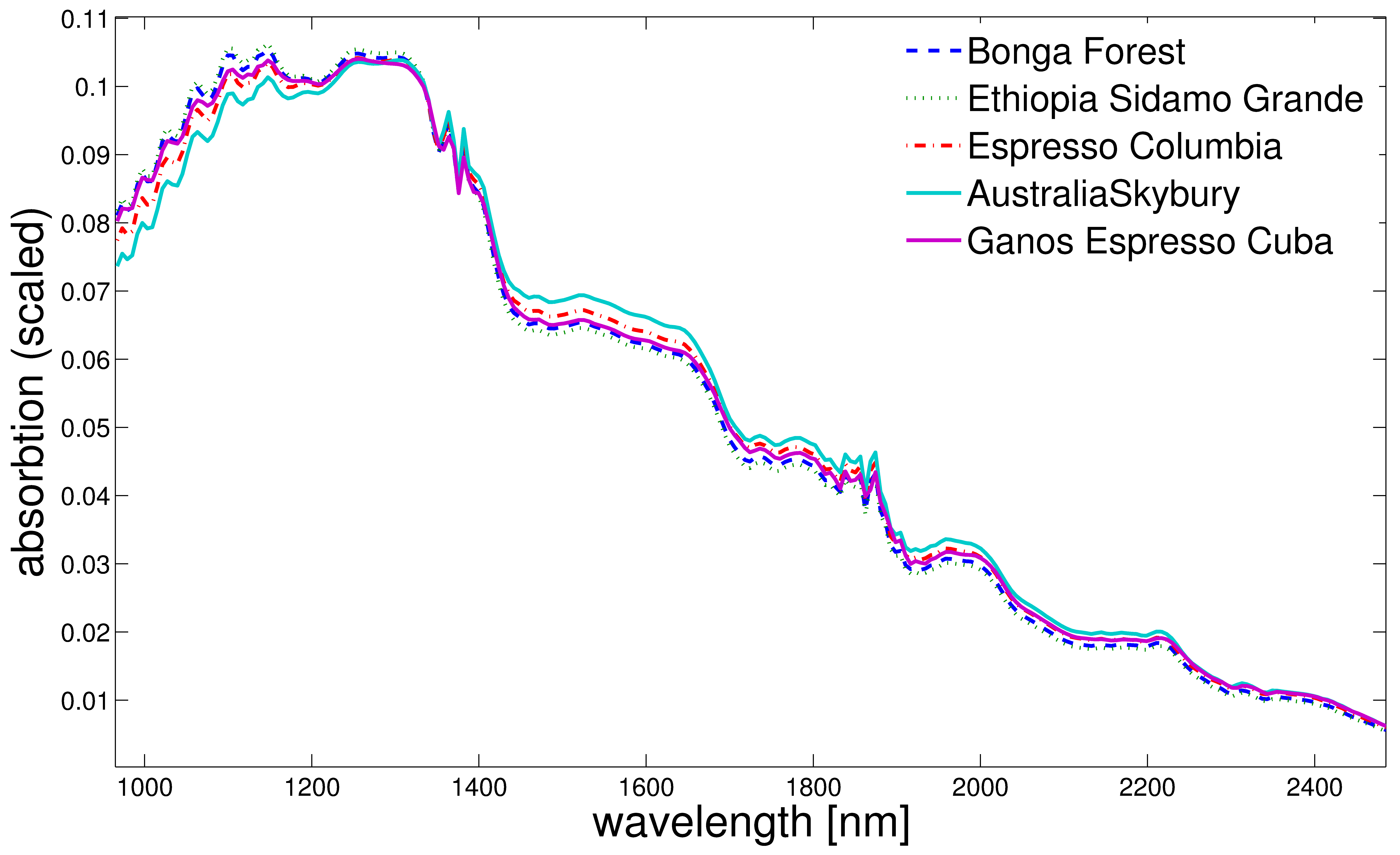
We applied the sparsity relevance learning model to classify hyperspectral short-wave infrared range (SWIR) spectral vectors of five coffee types. Hyperspectral processing along with an appropriate analysis of the acquired high-dimensional spectra has proven to be a suitable and very powerful method to quantitatively assess the biochemical composition of a wide range of biological samples [2]. By utilizing a hyperspectral camera (HySpex SWIR-$320$m-e, Norsk Elektro Optikk A/S) we obtained a rather extensive data base of spectra of five different coffee types ($5000$ spectra for each class). We used spectra in the SWIR between $970$ nm and $2,500$ nm at $6$ nm resolution yielding $256$ bands per spectrum. Proper image calibration was done by using a standard reflection pad (polytetrafluoroethylene, PTFE)[1]. After appropriate image segmentation the obtained spectra were normalized according to the $l_{2}$-norm and reduced to $200$ bands ignoring the range $2,000-2,500$ nm. The mean spectra of the five types are visualized in Fig. 1.

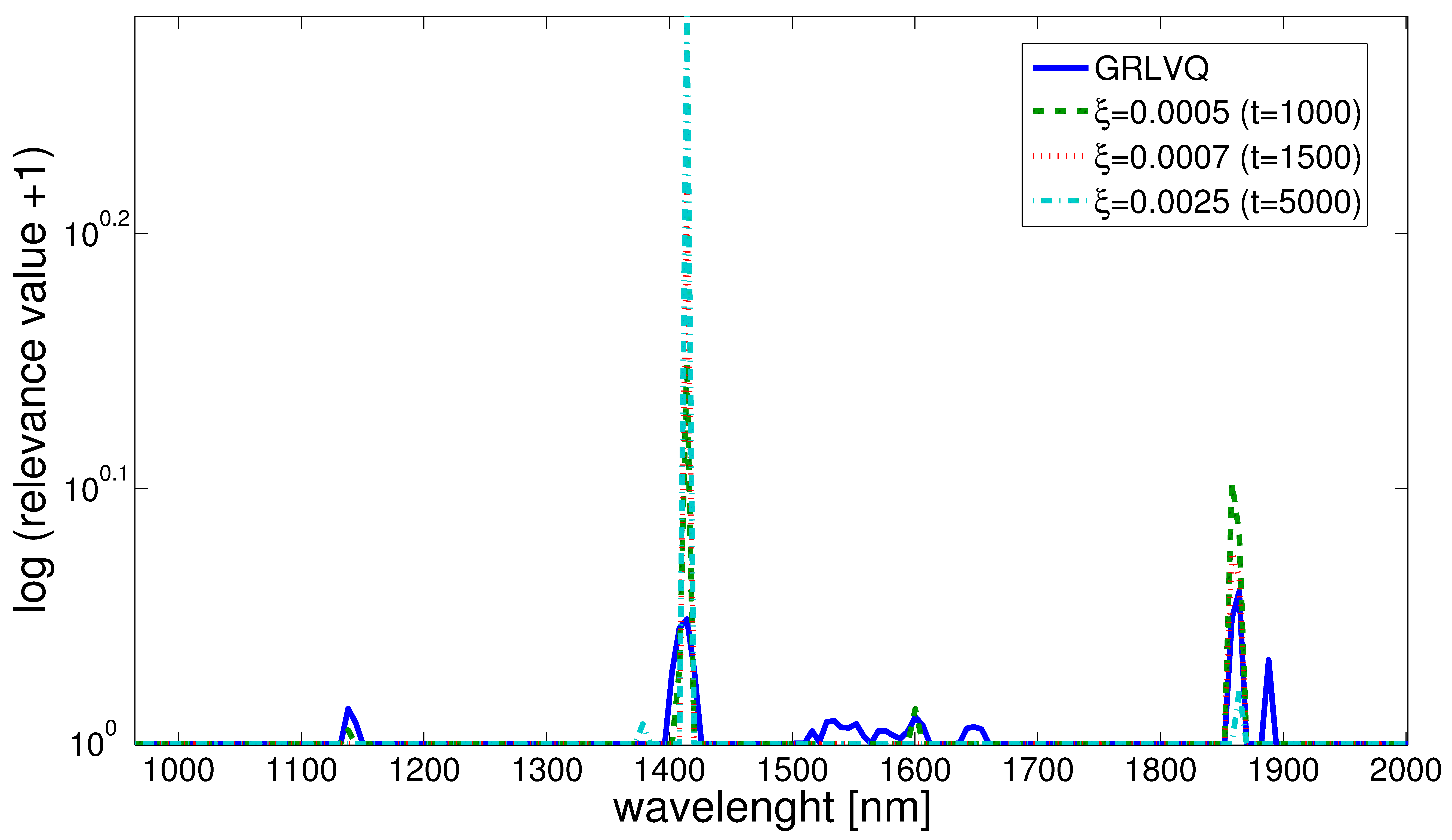
After standard training the GRLVQ model with full relevance profile yields $83,96\%$ accuracy. Starting with this solution the LASSO-model (7) was applied with linearly increasing weighting factor $\xi$ of the regularization term, the approximation parameter $\alpha$ in (9) was set constant $\alpha=5$. We compare this LASSO-approach with a sparsity model based on an entropy penalty term added to the cost function of GRLVQ as suggested in [8]. Both models enforce the sparsity of the relevance profiles. We depict the results of the LASSO approach Fig. 2, the other result is similar and has dropped because the lack of space.

Figure 2: Development of the sparsity of the relevance profile during LASSO-learning. With increasing influence of the regularization term the profile becomes sparse.

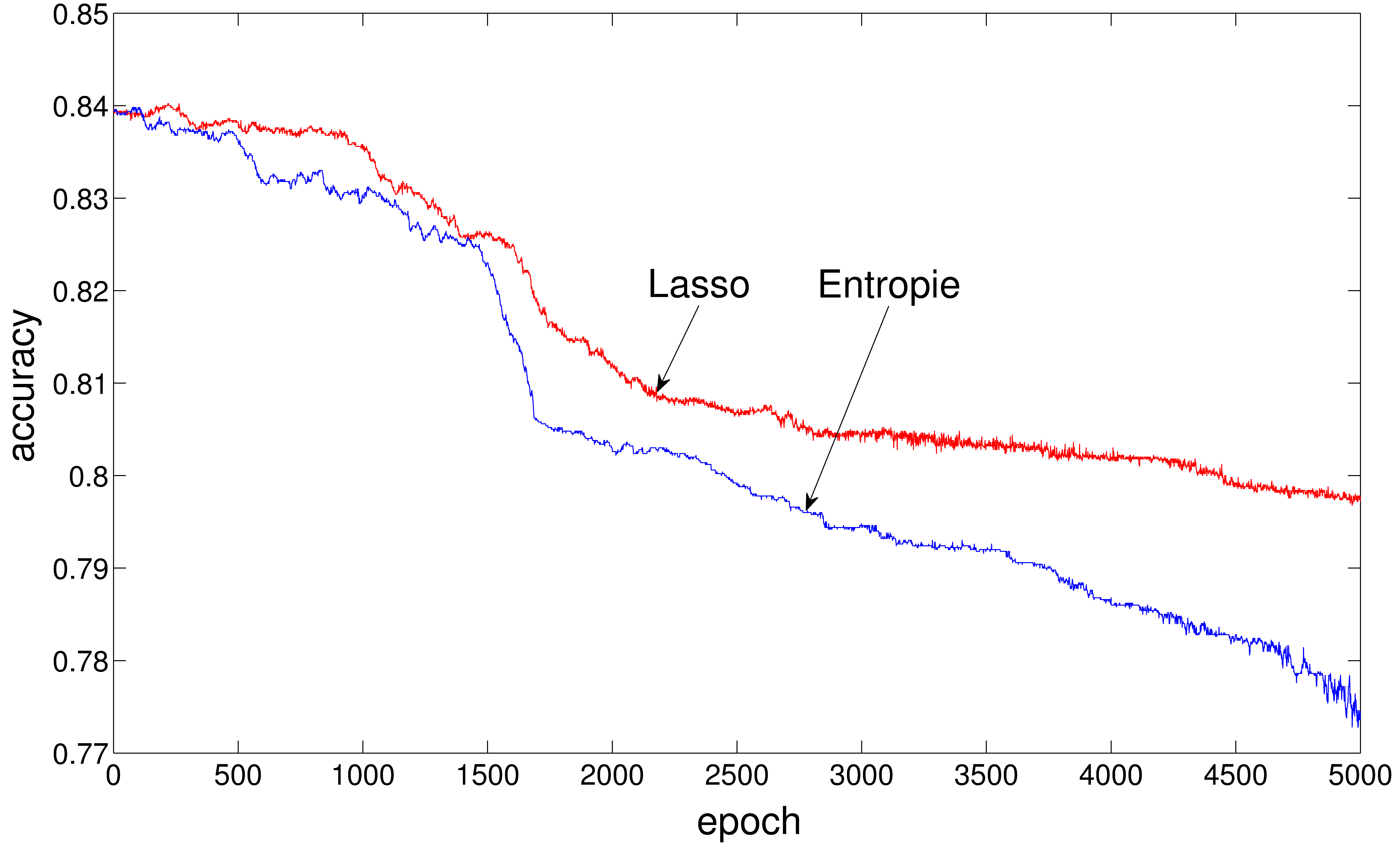
However, the accuracy decrease differs. LASSO keeps longer a high accuracy than the entropy approach, see Fig. 3 .

Figure 3: Development of the accuracies during sparsity adaptation according LASSO (red) and entropy based (blue) regularization. We observe instabilities of the entropy based method in the final phase of regularization.

Moreover, the entropy based method shows heavy instabilities if the relevance weights for spectral bands approach zero values at the end of the regularization process.

5 Conclusion

Sparsity in hyperspectral data analysis play an important role to concentrate on those bands, which are important for classification. Relevance learning as proposed in GRLVQ offers a possibility to weight the bands. However, frequently it delivers small but non-vanishing weights. Additional regularization can help to obtain sparse models. We have shown in this contribution that LASSO $l_{1}$-regularization can be applied in gradient based online learning using a differentiable approximation. We illustrate the method for an exemplary application of coffee classification based on hyperspectral signatures.

References

- [1] A. Backhaus, F. Bollenbeck, and U. Seiffert. High-throughput quality control of coffee varieties and blends by artificial neural networks and hyperspectral imaging. In Proceedings of the 1st International Congress on Cocoa, Coffee and Tea, CoCoTea 2011, page accepted for publication, 2011.
- [2] A. Backhaus, F. Bollenbeck, and U. Seiffert. Robust classification of the nutrition state in crop plants by hyperspectral imaging and artificial neural networks. In Proceedings of the 3rd IEEE Workshop on Hyperspectral Imaging and Signal Processing: Evolution in Remote Sensing WHISPERS 2011, page 9. IEEE Press, 2011.
- [3] K. Bunte, P. Schneider, B. Hammer, F.-M. Schleif, T. Villmann, and M. Biehl. Limited rank matrix learning, discriminative dimension reduction and visualization. Neural Networks, 26(1):159–173, 2012.
- [4] C. Chen and O. Mangasarian. Smoothing methods for convex inequalities and linear complementarity problems. Mathematical Programming, 71(1):51–69, 1995.
- [5] K. Crammer, R. Gilad-Bachrach, A.Navot, and A.Tishby. Margin analysis of the LVQ algorithm. In S. Becker, S. Thrun, and K. Obermayer, editors, Advances in Neural Information Processing (Proc. NIPS 2002), volume 15, pages 462–469, Cambridge, MA, 2003. MIT Press.
- [6] B. Hammer and T. Villmann. Generalized relevance learning vector quantization. Neural Networks, 15(8-9):1059–1068, 2002.
- [7] T. Hastie, R. Tibshirani, and J. Friedman. The Elements of Statistical Learning. Springer Verlag, Heidelberg-Berlin, 2001.
- [8] M. Kästner, B. Hammer, M. Biehl, and T. Villmann. Functional relevance learning in generalized learning vector quantization. Neurocomputing, 90(9):85–95, 2012.
- [9] T. Kohonen. Self-Organizing Maps, volume 30 of Springer Series in Information Sciences. Springer, Berlin, Heidelberg, 1995. (Second Extended Edition 1997).
- [10] A. Sato and K. Yamada. Generalized learning vector quantization. In D. S. Touretzky, M. C. Mozer, and M. E. Hasselmo, editors, Advances in Neural Information Processing Systems 8. Proceedings of the 1995 Conference, pages 423–9. MIT Press, Cambridge, MA, USA, 1996.
- [11] M. Schmidt, G. Fung, and R. Rosales. Fast optimization methods for l1 regularization: A comparative study and two new approaches. In J. Kok, J. Koronacki, R. Mantaras, S. Matwin, D. Mladenič, and A. Skowron, editors, Machine Learning: ECML 2007, volume 4701 of Lecture Notes in Computer Science, chapter 28, pages 286–297. Springer Berlin Heidelberg, Berlin, Heidelberg, 2007.
- [12] P. Schneider, K. Bunte, H. Stiekema, B. Hammer, T. Villmann, and M. Biehl. Regularization in matrix relevance learning. IEEE Transactions on Neural Networks, 21(5):831–840, 2010.
- [13] P. Schneider, B. Hammer, and M. Biehl. Adaptive relevance matrices in learning vector quantization. Neural Computation, 21:3532–3561, 2009.
- [14] R. Tibshirani. Regression shrinkage and selection via the lasso. Journal of the Royal Statistical Society: Series B, 58(1):267–288, 1996.