NEUTRON–PROTON PAIRS IN NUCLEI

Abstract

A review is given of attempts to describe nuclear properties in terms of neutron–proton pairs that are subsequently replaced by bosons. Some of the standard approaches with low-spin pairs are recalled but the emphasis is on a recently proposed framework with pairs of neutrons and protons with aligned angular momentum. The analysis is carried out for general $j$ and applied to $N=Z$ nuclei in the $1f_{7/2}$ and $1g_{9/2}$ shells.

PACS numbers: 03.65.Fd,21.60.Cs, 21.60.Ev

1 Introduction

In dealing with complex systems with many elementary components, one of the major goals of physics is to seek simplifications by adopting a description in terms of composite structures. An obvious example of this approach is found in nuclear physics, when the elementary constituents of the nucleus, quarks, are lumped into nucleons—an approximation adequate for the description of most nuclear phenomena at low energy. Still, the nuclear many-body problem in terms of nucleons instead of quarks is fiendishly difficult to solve for all but the lightest of nuclei, and further simplifying assumptions are required for the majority of them. One possibility is to lump the nucleons into pairs and attempt a description of nuclear phenomena in terms of those.

While such nucleon-pair models can be simple and attractive in principle, their success obviously depends on the type of pairs considered. This choice should be guided by nature of the interaction between the nucleons. One of the defining features of the nuclear force is that it is strongly attractive between nucleons that are paired to angular momentum $J=0$. Models where the pairing component of the interaction is prominent therefore have played an important part in the development of our understanding of nuclear structure [1]. While pairs consisting of identical nucleons (i.e., neutron–neutron or proton–proton) are by now an accepted feature of nuclei, much debate still exists concerning the role of neutron–proton pairs. One component of neutron–proton pairing is of isovector character, and arguments of isospin symmetry require that it should be considered on the same footing as its neutron–neutron or proton–proton equivalent. A neutron and a proton can also interact via an isoscalar component of the nuclear force and the debate is whether pairing of this type leads to enhanced collectivity and correlated states. This question is still unanswered after several decades of research [2, 3, 5, 4, 6, 7, 8]. A recent review of possible signatures of isoscalar neutron–proton pairing is given by Macchiavelli [9].

This paper certainly does not give a comprehensive and exhaustive review of the role of neutron–proton pairs in nuclei. Rather, it zooms in on a particular approach which replaces pairs of nucleons by bosons—approximation known under the name of ‘interacting boson model’— and within this class of models attention is paid to those that adopt bosons that stem from neutron–proton pairs. The standard boson models of this kind are briefly described in Sect. 2 but the emphasis is on a recently proposed framework with bosons that correspond to neutron–proton pairs with aligned, high angular momentum. The motivation for and the historical context of this new approach are outlined in Sect. 3. The main purpose of the present review is to argue that the proper framework to develop this approach is by applying boson mapping techniques to the nucleon-pair shell model. Technical aspects are reviewed in Sects. 4 and 5 while Sect. 6 gives a non-technical summary of the various approximations that enter a description in terms of aligned neutron–proton pairs or bosons. Applications to the $1f_{7/2}$ and $1g_{9/2}$ shells are discussed in Sect. 7. In fact, most of the results shown in that section are new and in this sense the present paper is not a review of published research. Nevertheless, it is the opinion of the author that they clarify the issue of the role in nuclei of neutron–proton pairs, aligned or otherwise. Finally, conclusions are drawn in Sect. 8.

2 Standard boson models with neutron–proton pairs: IBM-3 and IBM-4

The interacting boson model (IBM) of Arima and Iachello [10] starts from the premise that low-lying collective excitations can be described in terms of nucleon pairs (with angular momentum $0$ and $2$, in the most elementary version of the model) and that these pairs can be approximated as ($s$ and $d$) bosons. If neutrons and protons occupy different valence shells, it is natural to consider neutron–neutron and proton–proton pairs only, and to include the neutron–proton interaction as a force between the two types of pairs. This then leads to a version of the IBM with two kinds of bosons [11], of neutron and of proton type, the so-called IBM-2. If neutrons and protons occupy the same valence shell, this approach is no longer valid since there is no reason not to include a neutron–proton pair with isospin $T=1$. The version of the IBM that also contains the $T=1$ neutron–proton boson, proposed by Elliott and White [12], is called IBM-3. Because the IBM-3 includes the complete $T=1$ triplet, it can be made isospin invariant, enabling the construction of states with good total angular momentum $J$ and good total isospin $T$ and leading therefore to a more direct comparison with the shell model (see, e.g., Ref. Thompson87).

The bosons of the IBM-3 all have isospin $T=1$ and, in principle, other bosons can be introduced, in particular those that correspond to $T=0$ neutron–proton pairs. This further extension (proposed by Elliott and Evans [14] and referred to as IBM-4) is the most elaborate version of the standard IBM. The bosons are assigned an orbital angular momentum $L$, a spin $S$ and an isospin $T$, and in IBM-4 the choice $L=0$ and $L=2$ is retained with either $(S,T)=(0,1)$ or $(S,T)=(1,0)$. The total angular momentum $J$ of the bosons is obtained by coupling $L$ and $S$, leading to an ensemble of bosons with $(J,T)=(0,1)$, $(2,1)$, $(1,0)^{2}$, $(2,0)$ and $(3,0)$.

Figure 1: The energy spectrum of a neutron and a proton in a $p$ shell, interacting through an attractive delta force. States with isospin $T=0$ ($T=1$) are shown on the left (right). Levels are labelled on the left by $(S,T)L$, the spin $S$, the isospin $T$ and the orbital angular momentum $L$, and on the right by the angular momentum and parity $J^{\pi}$. All these quantum numbers are conserved in the absence of a spin–orbit splitting (left) while only the $J^{\pi}$ symmetry remains for a non-zero spin–orbit splitting (right).

The justification of this particular choice of bosons is based on the shell model. Consider as an example a neutron and a proton in a $p$ shell. The effective force between the two nucleons is of a short-range nature and can, within a reasonable approximation, be represented as an attractive delta interaction, $\hat{V}(\bar{r}_{1}-\bar{r}_{2})=-g\delta(\bar{r}_{1}-\bar{r}_{2})$ with $g>0$. Under the assumption of zero spin–orbit splitting (i.e., degenerate $p_{1/2}$ and $p_{3/2}$ shells), the energy spectrum can be worked out on the basis of simple symmetry arguments (see Fig. 1). Since the interaction is spin and isospin independent, the $LS$ coupling scheme applies and all states can be assigned an orbital angular momentum $L$, a spin $S$ and an isospin $T$. Furthermore, because of overall anti-symmetry, all states are characterized by either spatial symmetry ($L=0$ or 2) and spin–isospin anti-symmetry [$(S,T)=(0,1)$ or $(1,0)$], or spatial anti-symmetry ($L=1$) and spin–isospin symmetry [$(S,T)=(0,0)$ or $(1,1)$]. The former states are lowered in energy by the attractive delta force ($L=0$ more so than $L=2$) while the interaction energy in the latter states is exactly zero because of their spatial anti-symmetry. The states lowered in energy are precisely those that correspond to the bosons in IBM-4. For a realistic choice of spin–orbit splitting, the many degeneracies are lifted, lowering the higher-$J$ levels in energy (see Fig. 1). The choice of bosons in IBM-4 allows a classification where states carry the quantum numbers of total orbital angular momentum $L$, total spin $S$, total angular momentum $J$ and total isospin $T$, in addition to the SU(4) labels $(\lambda,\mu,\nu)$ of Wigner’s supermultiplet scheme [15], in close analogy with the corresponding shell-model labels.

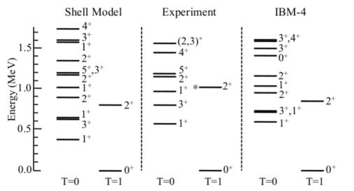
Figure 2: The spectrum of states in ⁶²Ga with isospin $T=0$ and $T=1$. Levels are labelled by their angular momentum and parity $J^{\pi}$. The different columns contain the results of a large-scale shell-model calculation [22], of a mapped IBM-4 calculation [23] and the experimental levels [24]. Figure taken from David et al. [24].

These qualitative arguments in favour of the IBM-4 have been corroborated by quantitative, microscopic studies in even–even [16] and odd–odd [17] $sd$-shell nuclei. In heavier nuclei the situation is more complex. The effect of the spin–orbit force is such that the $LS$-coupling scheme no longer applies, resulting in the breaking of the $L$ and $S$ quantum numbers, in contrast to the total angular momentum $J$ which is of course exactly conserved because of rotational invariance and the total isospin $T$ which conserved to a good approximation. Nevertheless, the $L$ and $S$ quantum numbers of the shell model can be replaced by their ‘pseudo’ equivalents, along the original ideas of Hecht and Adler [18], and Arima et al. [19]. This might be possible in specific regions of the nuclear chart [20] and is borne out by shell-model calculations with realistic interactions in nuclei beyond ⁵⁶Ni [21]. The existence of these approximate symmetries in the shell model allows a mapping onto IBM-4. A typical example is provided by the $N=Z$ nucleus ⁶²Ga. The spectroscopy predicted in the shell model, with a space consisting of the orbits $2p_{3/2}$, $1f_{5/2}$, $2p_{1/2}$ and $1g_{9/2}$, is very complex with intertwined states of isospin $T=0$ and $T=1$ [22]. Most levels are of low spin and those are well reproduced in the mapped IBM-4 calculation [23]. It is also found, however, that $T=0$ levels with higher spin ($5^{+}$, $6^{+}$ and $7^{+}$) are at significantly higher energies in the IBM-4 or even absent from it. This result is not surprising since the standard IBM-4 choice consists of bosons with rather low spin (up to $J^{\pi}=3^{+}$). In a recent experiment, David et al. [24] have observed a number of additional levels of low spin, presumably with isospin $T=0$, as predicted by the shell model and the IBM-4 (see Fig. 2). It remains nevertheless true that states with higher spin require an approach which is different from the standard IBM-4.

3 Aligned neutron–proton pairs

In a recent paper, Cederwall et al. [25] propose an alternative description of $N\sim Z$ nuclei in terms of neutron–proton pairs with aligned spin, henceforth referred to as $B$ pairs. The proposal concerns massive $N\sim Z$ nuclei, such as ⁹²Pd, approaching ¹⁰⁰Sn, with valence nucleons dominantly in the $1g_{9/2}$ shell. The claim is made (see also Refs. Qi11 and Xu12) that low-lying yrast states in ⁹²Pd and neighbouring nuclei are mainly built out of aligned neutron–proton isoscalar (with isospin $T=0$) pairs with angular momentum $J=9$. For the purpose of constructing a boson model, the aligned-pair scheme is particularly attractive since it involves a single neutron–proton pair; if valid, the many bosons of IBM-4 can be replaced by a single one.

Related ideas have been explored in the past. One is the stretch scheme of Danos and Gillet [28, 29] which applies to even–even $N=Z$ nuclei. It assumes that half of the neutrons align with half of the protons to form a state of maximum angular momentum. Similarly, the other half of the nucleons aligns to a state with the same angular momentum. The total angular momentum of the system is generated by the coupling of these two fixed stretched configurations. For four nucleons the stretch scheme is exactly equivalent to the description in terms of aligned pairs as proposed by Blomqvist and co-workers [25]. For eight, twelve,…nucleons, however, the stretch scheme is different since any angular momentum is uniquely defined in terms of the two stretch configurations while it generally can be written in several ways in terms of $B$ pairs. As a result, the stretch scheme has less flexibility to provide an adequate approximation of a realistic shell-model wave function. An explicit relation between both approximations is established in Sect. 7.

Blomqvist’s aligned $B$ pairs are in fact identical to the ‘$q$ pairs’ introduced in the 1980s by Daley. A $q$-pair analysis of the $1f_{7/2}$ shell with a schematic delta interaction exists as a Daresbury preprint [30] but, unfortunately, not as a published paper. The study of Daley concentrates on the even–even nuclei ⁴⁴Ti and ⁴⁸Cr, and only in the former nucleus does he find results similar to the ones shown below. No analysis of odd–odd nuclei is presented.

A crucial issue in any model that represents a fermionic system in terms of pairs (or, more generally, clusters) of fermions is the representation of exchange effects resulting from the Pauli principle as interactions between these clusters. In the stretch scheme of Danos and Gillet [28, 29] anti-symmetry between the two stretched configurations is neglected while it is not clear from Daley’s paper [30] to what extent the interactions between his $q$ bosons include Pauli effects. On the other hand, anti-symmetry is fully taken into account in the multi-step shell-model approach of Qi et al. [26], at the expense of major computational complexities which hinder an easy, intuitive interpretation of the results. One of the aims of this review is to analyze results of shell-model calculations in terms of $B$ pairs with the nucleon-pair shell model. Although numerically challenging, in particular for $B$ pairs in view of their high angular momentum, this approach provides a conceptually simple way to treat Pauli exchange effects between the pairs and subsequently represent those as interactions between bosons. The technical aspects of this approach are reviewed in the next two sections.

4 Nucleon-pair shell model

The natural framework to test Blomqvist’s truncation idea is provided by the nucleon-pair shell model (NPSM) [31, 32]. In the NPSM a basis is constructed from nucleon pairs. These can be collective superpositions of two-particle states or they may be identified with pure two-particle states themselves. The many applications of this formalism are reviewed in Ref. Zhao13un. The extension of the NPSM that includes isospin [34] is of particular relevance here.

In the language and notation of the NPSM, Blomqvist’s idea can be summarized with the statement that the full $T=0$ shell-model space can be reduced to one constructed out of aligned neutron–proton pairs of which the basis states are written as

$$|B^{n}L_{2}\dots L_{n}\rangle\equiv\left(\cdots\left(\left(B^{\dagger}\times B^{\dagger}\right)^{(L_{2})}\times B^{\dagger}\right)^{(L_{3})}\times\cdots\times B^{\dagger}\right)^{(L_{n})}|{\rm o}\rangle,$$ (1)

with $|{\rm o}\rangle$ the vacuum state. Pairs with angular momentum $J$ and projection $M_{J}$, and with isospin $T$ and projection $M_{T}$ are denoted by

$$P^{\dagger}_{JM_{J}TM_{T}}\equiv(a^{\dagger}_{jt}\times a^{\dagger}_{jt})^{(JT)}_{M_{J}M_{T}},$$ (2)

where $a^{\dagger}_{jm_{j}tm_{t}}$ creates a nucleon with angular momentum $j$ and projection $m_{j}$, and isospin $t=\frac{1}{2}$ and projection $m_{t}$. The short-hand notation $B^{\dagger}_{M_{J}}$ ($B$ for Blomqvist) is used in Eq. (1) for a creation operator of a neutron–proton pair with angular momentum $J=2j$ and isospin $T=0$. The $2n$-particle state (1) is characterized by the intermediate angular momenta $L_{2},\dots,L_{n}$, where $L_{n}$ is the final and total angular momentum of the state. In the basis (1) all pairs have $T=0$ and the coupling in isospin need not be considered.

The basis (1) is non-orthogonal and possibly overcomplete. Any calculation in this basis must therefore start from the diagonalization of the overlap matrix

$$\langle B^{n}_{i}|B^{n}_{i^{\prime}}\rangle\equiv\langle B^{n}L_{2}\dots L_{n-1}L_{n}|B^{n}L^{\prime}_{2}\dots L^{\prime}_{n-1}L_{n}\rangle,$$ (3)

where in bra and ket of the matrix element all possible intermediate angular momenta $L_{2},\dots,L_{n-1}$ must be considered, leading to a series of basis states denoted as $|B^{n}_{i}\rangle$ where $i$ is a short-hand notation for the set $\{L_{2},\dots,L_{n-1}\}$. The computation of the matrix elements (3) is complicated but possible with the recurrence relation devised by Chen [32]. Vanishing eigenvalues of the overlap matrix $\langle B^{n}_{i}|B^{n}_{i^{\prime}}\rangle$ indicate the overcompleteness of the pair basis. If a selection of $\omega$ pair-basis states is made for which all eigenvalues of the overlap matrix are non-zero, the following linear combinations can be constructed:

$$|\bar{B}^{n}_{k}\rangle=\sqrt{\frac{1}{o_{k}}}\sum_{i=1}^{\omega}c_{ki}|B^{n}_{i}\rangle,\qquad k=1,\dots,\omega,$$ (4)

where $o_{k}$ is the $k^{\rm th}$ eigenvalue of the overlap matrix and $c_{ki}$ $(i=1,\dots,\omega)$ the associated eigenvector. The vectors $|\bar{B}^{n}_{k}\rangle$ $(k=1,\dots,\omega)$ are normalized, orthogonal and linearly independent, and therefore provide a proper basis for a shell-model calculation, albeit a truncated one. For a given shell-model hamiltonian $\hat{H}^{\rm f}$, the energy spectrum and eigenvectors can be obtained from the diagonalization of the matrix

$$\langle\bar{B}^{n}_{k}|\hat{H}^{\rm f}|\bar{B}^{n}_{k^{\prime}}\rangle=\sqrt{1\over{o_{k}o_{k^{\prime}}}}\sum_{i,i^{\prime}=1}^{\omega}c_{ki}c_{k^{\prime}i^{\prime}}\langle B^{n}_{i}|\hat{H}^{\rm f}|B^{n}_{i^{\prime}}\rangle,\qquad k,k^{\prime}=1,\dots,\omega.$$ (5)

The formalism as explained so far allows one to perform a shell-model calculation in a truncated basis constructed from aligned $T=0$ neutron–proton pairs. In subsequent applications we will also want to analyze arbitrary shell-model wave functions in terms of $B$ pairs. An analysis of this type clearly cannot be carried out in the basis (1)—since the latter spans only part of the shell-model space—and it requires a generalization to a basis in terms of arbitrary pairs. The formalism of the NPSM with isospin, needed to this end, is detailed in Ref. Fu13a and only a few basic formulas are given here.

It is convenient to introduce the following short-hand notation for the pairs:

$$P^{\dagger}_{\Gamma M_{\Gamma}}\equiv P^{\dagger}_{JM_{J}TM_{T}}\equiv(a^{\dagger}_{\gamma}\times a^{\dagger}_{\gamma})^{(\Gamma)}_{M_{\Gamma}}\equiv(a^{\dagger}_{jt}\times a^{\dagger}_{jt})^{(JT)}_{M_{J}M_{T}},$$ (6)

where $\gamma$ stands for $jt$, $\Gamma$ for $JT$, $m_{\gamma}$ for $m_{j}m_{t}$ and $M_{\Gamma}$ for $M_{J}M_{T}$. An arbitrary pair state can then be written as

$$|\Gamma_{1}\dots\Gamma_{n}\Lambda_{2}\dots\Lambda_{n}\rangle\equiv\left(\cdots\left(\left(P_{\Gamma_{1}}^{\dagger}\times P_{\Gamma_{2}}^{\dagger}\right)^{(\Lambda_{2})}\times P_{\Gamma_{3}}^{\dagger}\right)^{(\Lambda_{3})}\times\cdots\times P_{\Gamma_{n}}^{\dagger}\right)^{(\Lambda_{n})}|{\rm o}\rangle,$$ (7)

which can be denoted in short as

$$|P^{n}_{j}\rangle\equiv|\Gamma_{1}\dots\Gamma_{n}\Lambda_{2}\dots\Lambda_{n}\rangle,$$ (8)

where the index $j$ stands for the set $\{\Gamma_{1}\dots\Gamma_{n}\Lambda_{2}\dots\Lambda_{n-1}\}$, that is, the angular momenta and isospins $\Gamma_{q}$ of the $n$ pairs, and the intermediate angular momenta and isospins $\Lambda_{q}$. Note that $\Lambda_{1}$ (not shown) equals $\Gamma_{1}$ and that $\Lambda_{n}$ is the total angular momentum and isospin, and therefore fixed and not included in $j$. Since Chen’s algorithm [32] is valid for arbitrary pairs, the analysis now proceeds as before, and consists of the construction of an orthonormal basis from the diagonalization of the overlap matrix $\langle P^{n}_{j}|P^{n}_{j^{\prime}}\rangle$,

$$|\bar{P}^{n}_{r}\rangle=\sqrt{1\over{O_{r}}}\sum_{j=1}^{\Omega}C_{rj}|P^{n}_{j}\rangle,\qquad r=1,\dots,\Omega,$$ (9)

where $O_{r}$ and $C_{rj}$ have the same meaning as in Eq. (4) but now in the full shell-model basis of dimension $\Omega$. The diagonalization of the shell-model hamiltonian in that basis,

$$\langle\bar{P}^{n}_{r}|\hat{H}^{\rm f}|\bar{P}^{n}_{r^{\prime}}\rangle=\sqrt{1\over{O_{r}O_{r^{\prime}}}}\sum_{j,j^{\prime}=1}^{\Omega}C_{rj}C_{r^{\prime}j^{\prime}}\langle P^{n}_{j}|\hat{H}^{\rm f}|P^{n}_{j^{\prime}}\rangle,\qquad r,r^{\prime}=1,\dots,\Omega,$$ (10)

leads to the untruncated eigenspectrum of the shell model.

The $B$-pair content of an arbitrary shell-model state can now be analyzed as follows. First, a shell-model diagonalization is performed in a complete basis $|\bar{P}^{n}_{r}\rangle$ $(r=1,\dots,\Omega)$, leading to eigenstates

$$|\bar{E}^{n}_{s}\rangle=\sum_{r=1}^{\Omega}E_{sr}|\bar{P}^{n}_{r}\rangle,\qquad s=1,\dots,\Omega.$$ (11)

The $B$-pair content of a given eigenstate $|\bar{E}^{n}_{s}\rangle$ is the square of its projection onto the subspace spanned by $B$-pair states which equals

$$\langle\bar{E}^{n}_{s}|B^{n}\rangle^{2}\equiv\sum_{k=1}^{\omega}|\langle\bar{E}^{n}_{s}|\bar{B}^{n}_{k}\rangle|^{2},$$ (12)

where the overlap matrix element on the right-hand side can expressed as

$$\langle\bar{E}^{n}_{s}|\bar{B}^{n}_{k}\rangle=\sum_{r,j=1}^{\Omega}\sum_{i=1}^{\omega}E_{sr}\sqrt{\frac{1}{O_{r}}}C_{rj}\sqrt{\frac{1}{o_{k}}}c_{ki}\langle P^{n}_{j}|B^{n}_{i}\rangle,$$ (13)

in terms of overlap matrix elements that can be computed with Chen’s algorithm [32].

A final word is needed concerning the calculation of matrix elements of a shell-model hamiltonian between pair states as they appear on the right-hand sides of Eqs. (5) and (10). For the case of a single-$j$ shell, the one-body part of $\hat{H}^{\rm f}$ gives rise to a constant and can be neglected. Its two-body part $\hat{H}^{\rm f}_{2}$ is entirely determined by the two-body matrix elements

$$\upsilon^{2\rm f}_{\Gamma}\equiv\upsilon^{2\rm f}_{JT}\equiv\langle j^{2}JT|\hat{H}^{\rm f}_{2}|j^{2}JT\rangle,$$ (14)

which enter as follows in the expression for the pair matrix element:

$$\langle\Gamma_{1}\dots\Gamma_{n}\Lambda_{2}\dots\Lambda_{n}|\hat{H}^{\rm f}_{2}|\Gamma^{\prime}_{1}\dots\Gamma^{\prime}_{n}\Lambda^{\prime}_{2}\dots\Lambda^{\prime}_{n}\rangle$$ (15)

$$= \delta_{\Lambda_{n}\Lambda^{\prime}_{n}}\left[\frac{4n-2\gamma-1}{2\gamma+1}\langle\Gamma_{1}\dots\Gamma_{n}\Lambda_{2}\dots\Lambda_{n}|\Gamma^{\prime}_{1}\dots\Gamma^{\prime}_{n}\Lambda^{\prime}_{2}\dots\Lambda^{\prime}_{n}\rangle\sum_{\Gamma}(2\Gamma+1)\upsilon^{2\rm f}_{\Gamma}+\right.$$

$$\left.\sum_{\Gamma\Lambda}\frac{2\Lambda+1}{2(2\Lambda_{n}+1)}\langle\Gamma_{1}\dots\Gamma_{n}\Gamma\Lambda_{2}\dots\Lambda_{n}\Lambda|\Gamma^{\prime}_{1}\dots\Gamma^{\prime}_{n}\Gamma\Lambda^{\prime}_{2}\dots\Lambda^{\prime}_{n}\Lambda\rangle\upsilon^{2\rm f}_{\Gamma}\right],$$

with $2\gamma+1=2(2j+1)$, $2\Gamma+1=(2J+1)(2T+1)$, $2\Lambda_{q}+1=(2L_{q}+1)(2T_{q}+1)$, and so on. The second sum is over all possible pairs with angular momentum and isospin $\Gamma$ which couples with $\Lambda_{n}$ to all possible $\Lambda$, the total angular momentum and isospin of the $(n+1)$-pair state.

It is well known [36] that the limitation to a restricted model space (e.g., a single-$j$ shell) leads to an effective hamiltonian with higher-order interactions (see Refs. 37 and 38 for a recent discussion of $T=1$ three-body interactions in the $1f_{7/2}$ shell). Equations (5) and (10) are generally valid, irrespective of the order of the interaction in $\hat{H}^{\rm f}$. Equation (15), on the other hand, is specific to a two-body interaction but it can be readily generalized to higher orders. The corresponding expression for a three-body interaction, for example, involves the same overlap matrix elements as those in Eq. (15) with in addition overlaps between states of $(n+1)$ pairs plus one particle. These can be computed with the NPSM algorithm generalized to odd-mass nuclei [39].

In the present review the order of the interactions in the shell-model hamiltonian is limited to two-body and lowest-order transition operators are taken.

5 Boson mapping

The boson equivalent of the basis (1) is

$$|b^{n}L_{2}\dots L_{n}\rangle\equiv\left(\cdots\left(\left(b^{\dagger}\times b^{\dagger}\right)^{(L_{2})}\times b^{\dagger}\right)^{(L_{3})}\times\cdots\times b^{\dagger}\right)^{(L_{n})}|{\rm o}\rangle,$$ (16)

where $b^{\dagger}$ creates a boson with angular momentum (or spin) $\ell=2j$ and isospin $t=0$. While the angular momentum coupling is the same in Eqs. (1) and (16), overlap and hamiltonian matrix elements are different in both bases because of the internal structure of the pairs, in contrast to the assumed elementary character of the bosons. Nevertheless, Pauli corrections can be systematically applied to the boson calculation in the following way. In general, for $n>2$, the boson basis (16) is non-orthogonal and overcomplete. As in the fermion case, the diagonalization of the overlap matrix

$$\langle b^{n}_{i}|b^{n}_{i^{\prime}}\rangle\equiv\langle b^{n}L_{2}\dots L_{n-1}L_{n}|b^{n}L^{\prime}_{2}\dots L^{\prime}_{n-1}L_{n}\rangle,$$ (17)

leads to an orthogonal basis of linearly independent vectors. For technical reasons that have to do with the computation of coefficients of fractional parentage (CFPs), it is in this case more convenient to define an orthonormal basis via a Gram–Schmidt procedure. For a given sequence of linearly independent, non-orthogonal $n$-boson states $|b^{n}_{i}\rangle$ $(i=1,\dots,\omega^{\prime})$, an orthogonal series can be defined as follows:

$$|\tilde{b}^{n}_{1}\rangle = \langle b^{n}_{1}|b^{n}_{1}\rangle^{-1/2}|b^{n}_{1}\rangle,$$

$$|\tilde{b}^{n}_{2}\rangle = \bigl{(}\langle b^{n}_{2}|b^{n}_{2}\rangle-\langle b^{n}_{2}|\tilde{b}^{n}_{1}\rangle^{2}\bigr{)}^{-1/2}\bigl{(}|b^{n}_{2}\rangle-\langle b^{n}_{2}|\tilde{b}^{n}_{1}\rangle|\tilde{b}^{n}_{1}\rangle\bigr{)},$$

$$\vdots$$

$$|\tilde{b}^{n}_{i}\rangle = \left(\langle b^{n}_{i}|b^{n}_{i}\rangle-\sum_{j=1}^{i-1}\langle b^{n}_{i}|\tilde{b}^{n}_{j}\rangle^{2}\right)^{-1/2}\left(|b^{n}_{i}\rangle-\sum_{j=1}^{i-1}\langle b^{n}_{i}|\tilde{b}^{n}_{j}\rangle|\tilde{b}^{n}_{j}\rangle\right),$$ (18)

until $i=\omega^{\prime}$. To establish the connection with the orthogonal fermion-pair series, an additional transformation is needed,

$$|\bar{b}^{n}_{k}\rangle=\sum_{i=1}^{\omega}c_{ki}|\tilde{b}^{n}_{i}\rangle,\qquad k=1,\dots,\omega,$$ (19)

in terms of the coefficients $c_{ki}$ defined in Eq. (4). Because of the orthogonality of the basis $|\tilde{b}^{n}_{i}\rangle$ and the properties of the coefficients $c_{ki}$, the basis $|\bar{b}^{n}_{k}\rangle$ is orthogonal and is the boson equivalent of the fermion basis $|\bar{B}^{n}_{k}\rangle$. The matrix elements of the boson hamiltonian in this basis are therefore determined from

$$\langle\bar{b}^{n}_{k}|\hat{H}^{\rm b}|\bar{b}^{n}_{k^{\prime}}\rangle=\langle\bar{B}^{n}_{k}|\hat{H}^{\rm f}|\bar{B}^{n}_{k^{\prime}}\rangle,\qquad k,k^{\prime}=1,\dots,\omega.$$ (20)

With use of the inverse of the relation (19), of the equality (20) and of Eq. (5), the matrix elements of the boson hamiltonian in the orthogonal basis $|\tilde{b}^{n}_{i}\rangle$ can be written in terms of those of the shell-model hamiltonian in the fermion-pair basis,

$$\langle\tilde{b}^{n}_{i}|\hat{H}^{\rm b}|\tilde{b}^{n}_{i^{\prime}}\rangle=\sum_{k,k^{\prime}=1}^{\omega}\sqrt{\frac{1}{o_{k}o_{k^{\prime}}}}c_{ki}c_{k^{\prime}i^{\prime}}\sum_{j,j^{\prime}=1}^{\omega}c_{kj}c_{k^{\prime}j^{\prime}}\langle B^{n}_{j}|\hat{H}^{\rm f}|B^{n}_{j^{\prime}}\rangle,\qquad i,i^{\prime}=1,\dots,\omega.$$ (21)

Three additional technical issues must be ironed out. First, for a given total angular momentum $L_{n}$, the number of linearly independent boson states (16) may be larger than the corresponding number of fermion-pair states (1), $\omega\leq\omega^{\prime}$, indicating that there are $\omega^{\prime}-\omega$ spurious boson states which are Pauli forbidden in the fermion space. The matrix elements of the boson hamiltonian pertaining to these states remain undefined in Eq. (21). Since these states are spurious, they must be eliminated from the boson space, implying the following choice of boson matrix elements:

$$\langle\tilde{b}^{n}_{i}|\hat{H}^{\rm b}|\tilde{b}^{n}_{i}\rangle = +\infty,\qquad i=\omega+1,\dots,\omega^{\prime},$$

$$\langle\tilde{b}^{n}_{i}|\hat{H}^{\rm b}|\tilde{b}^{n}_{i^{\prime}}\rangle=\langle\tilde{b}^{n}_{i^{\prime}}|\hat{H}^{\rm b}|\tilde{b}^{n}_{i}\rangle = 0,\qquad i\leq\omega<i^{\prime}\leq\omega^{\prime}.$$ (22)

The second technical issue concerns the fact that Eq. (21) defines the entire boson hamiltonian up to and including $n$-body interactions. To isolate its $n$-body part $\hat{H}^{\rm b}_{n}$, one should subtract the previously determined $n^{\prime}$-body interactions, $n^{\prime}<n$. The procedure is straightforward but rather cumbersome to write down explicitly up to all orders. Up to the three-body interactions that will be considered below, one has the following results. The single-boson energy is determined from

$$\epsilon_{b}\equiv\langle b|\hat{H}^{\rm b}|b\rangle=\langle B|\hat{H}^{\rm f}|B\rangle,$$ (23)

which is nothing but the shell-model matrix element $\upsilon^{2\rm f}_{JT}$ in the aligned neutron–proton configuration with $J=2j$ and $T=0$. The two-body part of the boson hamiltonian is determined from

$$\upsilon^{2\rm b}_{L_{2}}\equiv\langle b^{2}L_{2}|\hat{H}^{\rm b}_{2}|b^{2}L_{2}\rangle=\langle b^{2}L_{2}|\hat{H}^{\rm b}|b^{2}L_{2}\rangle-2\epsilon_{b},$$ (24)

where it is assumed that the two-boson states are normalized such that the matrix element of the total boson hamiltonian can be taken from Eq. (21). The three-body part of the boson hamiltonian follows from

$$\langle b^{3}[\tilde{L}_{2}]L_{3}|\hat{H}^{\rm b}_{3}|b^{3}[\tilde{L}^{\prime}_{2}]L_{3}\rangle = \langle b^{3}[\tilde{L}_{2}]L_{3}|\hat{H}^{\rm b}|b^{3}[\tilde{L}^{\prime}_{2}]L_{3}\rangle-3\epsilon_{b}\delta_{\tilde{L}_{2}\tilde{L}^{\prime}_{2}}-$$ (25)

$$3\sum_{L^{\prime\prime}_{2}}[\ell^{2}[L^{\prime\prime}_{2}]\ell|\}\ell^{3}[\tilde{L}_{2}]L_{3}][\ell^{2}[L^{\prime\prime}_{2}]\ell|\}\ell^{3}[\tilde{L}^{\prime}_{2}]L_{3}]\upsilon^{2\rm b}_{L^{\prime\prime}_{2}},$$

where again the matrix element of the total boson hamiltonian on the right-hand side are calculated from Eq. (21). Equation (25) requires some explanation. The basis consisting of the three-boson states

$$|b^{3}L_{2}L_{3}\rangle\equiv\left(\left(b^{\dagger}\times b^{\dagger}\right)^{(L_{2})}\times b^{\dagger}\right)^{(L_{3})}|{\rm o}\rangle,$$ (26)

is non-orthogonal and non-normalized. The intermediate angular momentum $L_{2}$ can be used as a label and, after the application of Eq. (18), one arrives at an orthogonal basis denoted by $|b^{3}[\tilde{L}_{2}]L_{3}\rangle$, with the notation $[\tilde{L}_{2}]$ as a reminder of the Gram–Schmidt procedure. This basis can be used to express the matrix elements of a two-body interaction in the usual manner with CFPs [40]. In general, the matrix element of an $n^{\prime}$-body boson hamiltonian between $n$-boson states ($n\geq n^{\prime}$) can be written as

$$\langle\tilde{b}^{n}_{i}|\hat{H}^{\rm b}_{n^{\prime}}|\tilde{b}^{n}_{i^{\prime}}\rangle=\frac{n!}{n^{\prime}!(n-n^{\prime})!}\sum_{jkk^{\prime}}[\tilde{b}^{n-n^{\prime}}_{j}\tilde{b}^{n^{\prime}}_{k}|\}\tilde{b}^{n}_{i}][\tilde{b}^{n-n^{\prime}}_{j}\tilde{b}^{n^{\prime}}_{k^{\prime}}|\}\tilde{b}^{n}_{i^{\prime}}]\langle\tilde{b}^{n^{\prime}}_{k}|\hat{H}^{\rm b}_{n^{\prime}}|\tilde{b}^{n^{\prime}}_{k^{\prime}}\rangle,$$ (27)

in terms of $n\rightarrow n-n^{\prime}$ CFPs. The third term on the right-hand side of Eq. (25) arises from the application of this result for $n=3$ and $n^{\prime}=2$, together with the explicit notation of CFPs for bosons with spin $\ell$.

The third technical issue concerns the hierarchy of states since, in general, the definition of the interactions between the bosons depends on the order of states chosen in the Gram–Schmidt procedure (19). In the mapping from $B$ pairs to $b$ bosons no ambiguity exists for the two-body interaction between the bosons ($n=2$) since states are unique for a given angular momentum $J$. This is no longer the case for $n\geq 3$ and as a result there exist many different $n$-body interactions that exactly reproduce the shell-model results in the $B^{n}$ space. The method followed here is to define a hierarchy based on the importance of the overlap with the yrast shell-model state (see Sect. 7 for examples), leading to a procedure which, for $n=3$, can be summarized in the following steps.

• Construct and diagonalize the shell-model hamiltonian in the $B^{3}$ basis, leading to the eigenvalues $E_{k}$ ($k=1,\dots,\omega$).

• To deal with spurious states, the set of $\omega$ eigenvalues is enlarged with $E_{k}=+\infty$ ($k=\omega^{\prime}-\omega+1,\dots,\omega^{\prime}$) (i.e., $\omega^{\prime}-\omega$ large values in numerical applications).

• Construct and diagonalize the boson hamiltonian with up to two-body interactions in the analogue $b^{3}$ basis. This is achieved by computing the second and third terms on the left-hand side of Eq. (25) which after diagonalization yields the eigenvalues $E^{\prime}_{k}$ ($k=1,\dots,\omega^{\prime}$) with corresponding eigenvectors $c^{\prime}_{kl}$ ($l=1,\dots,\omega^{\prime}$).

• The three-body interaction in the analogue boson basis is obtained by transforming back the matrix with the differences $E_{k}-E^{\prime}_{k}$ on the diagonal,

  $$\upsilon^{3\rm b}_{ll^{\prime}}=\sum_{k=1}^{\omega^{\prime}}c^{\prime}_{lk}(E_{k}-E^{\prime}_{k})c^{\prime}_{kl^{\prime}},$$ (28)

  where $l$ and $l^{\prime}$ are short-hand notations for the three-boson labels $[\tilde{L}_{2}]L_{3}$ and $[\tilde{L}^{\prime}_{2}]L_{3}$.

Since the three-body components of the boson interaction are found to be small (see Sect. 7), no exhaustive study of the three-body aspect of the mapping is attempted in this review.

6 Three approximations

Let us now take stock of the situation with regard to the aligned-pair approximation as described in the technical discussion of the previous two sections. A first possibility is to determine the $T=0$ spectrum of a $2n$-particle system by diagonalizing a given shell-model hamiltonian $\hat{H}^{\rm f}$ in the aligned-pair basis $|\bar{B}^{n}_{k}\rangle$. This is a truncated shell-model calculation in which the Pauli principle is fully taken into account and no boson mapping is needed. The calculation becomes more difficult as $n$ increases because of the complexity of Chen’s algorithm. This truncated shell-model calculation can be replaced exactly by its boson equivalent if the mapped boson hamiltonian $\hat{H}^{\rm b}$ is determined up to all orders (i.e., up to order $n$ for a $2n$-particle system). The Pauli principle is obeyed by means of appropriate interactions between the bosons. No simplification of the original problem is obtained since the determination of $\hat{H}^{\rm b}$ up to order $n$ requires the calculation of matrix elements of $\hat{H}^{\rm f}$ in the aligned-pair basis $|B^{n}_{k}\rangle$ [see Eq. (21)]. Significant simplifications may result, however, if the mapped boson hamiltonian $\hat{H}^{\rm b}$ is determined up to an order $n^{\prime}<n$ but this simplification is at the expense of some violation of the Pauli principle.

In Sect. 7 the above statements are illustrated with examples. Since a number of approximations are made at different stages, it is useful to enounce these approximations and to indicate whether they can be tested theoretically and/or experimentally. Let us start from the general observation that the $N=Z$ nuclei under consideration can be described in the spherical shell model if a sufficiently large model space with an appropriate interaction is adopted. With this as a premise the following assumptions are made to arrive at an approximation in terms of aligned-pair bosons. [(iii)]

The shell-model space is truncated to a single high-$j$ orbit. A theoretical test of this assumption is not attempted in this review. Its validity clearly depends on the specific features of the initial shell-model hamiltonian. Two particular mass regions where the approximation might be valid spring to mind: $N=Z$ nuclei in the $1f_{7/2}$ and $1g_{9/2}$ shells. More important is that the assumption can be tested experimentally, as illustrated with examples in Sect. 7.

The single-$j$ shell space is reduced to one written in terms of aligned $B$ pairs. Some dependence exists on the shell-model interaction adopted in the single-$j$ shell space. Nevertheless, if a reasonable interaction is taken, this assumption can be tested generically. Furthermore, the extension of the NPSM that includes isospin [34] is the appropriate formalism to test the combined approximations (i) and (ii). A recent calculation of this type [35], which starts from a realistic shell-model space and interaction, seem to indicate that the combined approximations (i) and (ii) hold fairly well in $N=Z$ nuclei from ⁹²Pd to ¹⁰⁰Sn.

The aligned $B$ pairs are replaced by $b$ bosons. As argued in the previous section, if the boson hamiltonian is calculated up to all orders, the mapping is exact and no approximation is made. The usual procedure, however, is to map up to two-body boson interactions which implies some amount of Pauli violation. In the next section the validity of the two-body boson mapping is tested by calculating the effect of the three-body interaction.

7 Applications

A number of results can be established for a shell with arbitrary $j$ . They are useful in the discussion of specific cases, in particular the $1f_{7/2}$ and $1g_{9/2}$ shells.

7.1 Any $j$ shell

The M1 operator in the shell model is given by

$$\hat{T}^{\rm f}_{\mu}({\rm M1})=\sqrt{\frac{3}{4\pi}}\left(\sum_{i\in\nu}g^{s}_{\nu}s_{\mu}(i)+\sum_{i\in\pi}\left[g^{\ell}_{\pi}\ell_{\mu}(i)+g^{s}_{\pi}s_{\mu}(i)\right]\right),$$ (29)

where the sums are over neutrons and protons, and in each sum appear the orbital and spin gyromagnetic factors, $g^{\ell}_{\rho}$ and $g^{s}_{\rho}$, with $\rho=\nu$ for a neutron and $\rho=\pi$ for a proton. For the calculation of magnetic moments (i.e., diagonal matrix elements) the M1 operator (29) can be replaced by one in terms of neutron and proton $g$ factors. In second quantization the $z$ component of the latter operator can be written as

$$\hat{\mu}^{\rm f}_{0}=\sqrt{\frac{j(j+1)(2j+1)}{3}}\left[g_{\nu}(\nu^{\dagger}_{j}\times\tilde{\nu}_{j})^{(1)}_{0}+g_{\pi}(\pi^{\dagger}_{j}\times\tilde{\pi}_{j})^{(1)}_{0}\right],$$ (30)

where $\rho^{\dagger}_{jm}$ creates a neutron ($\rho=\nu$) or a proton ($\rho=\pi$) in the $j$ shell, and $\tilde{\rho}_{jm}=(-)^{j+m}\rho_{j-m}$. This operator can be written alternatively as a sum of an isoscalar part, multiplied by $(g_{\nu}+g_{\pi})$, and an isovector part, multiplied by $(g_{\nu}-g_{\pi})$. For the M1 matrix elements between states in a single-$j$ shell of the same isospin $T$ and with projection $T_{z}=0$, only the former part contributes and, since the isoscalar part is proportional to the angular momentum operator, it follows that the $g$ factor of any state in an $N=Z$ nucleus equals $(g_{\nu}+g_{\pi})/2$. This result is generally valid under the assumptions that isospin is a good quantum number and that the nucleons are confined to a single-$j$ shell [41].

In terms of $b$ bosons the M1 operator is of the form

$$\hat{T}^{\rm b}_{\mu}({\rm M1})=\sqrt{\frac{3}{4\pi}}g_{b}\hat{J}_{\mu}=\sqrt{\frac{2j(2j+1)(4j+1)}{4\pi}}g_{b}(b^{\dagger}\times\tilde{b})^{(1)}_{\mu}.$$ (31)

The $g$ factor of the $b$ boson, $g_{b}$, is obtained from the $g$ factor of the $B$ pair which, due to the above argument, equals $(g_{\nu}+g_{\pi})/2$. Since the operator (31) is proportional to the angular momentum operator, one finds that the $g$ factor of any state $|\alpha J\rangle$ in the boson model equals

$$g(\alpha J)\equiv\frac{\mu(\alpha J)}{J}=\sqrt{\frac{4\pi}{3}}\frac{\langle\alpha JJ|\hat{T}^{\rm b}_{0}({\rm M1})|\alpha JJ\rangle}{J}=g_{b}=\frac{g_{\nu}+g_{\pi}}{2}.$$ (32)

One recovers therefore the shell-model result that the $g$ factor of any state in an $N=Z$ nucleus equals $(g_{\nu}+g_{\pi})/2$.

The conclusion of the preceding discussion is that magnetic moments do not provide a test of the assumptions (ii) and (iii) of Sect. 6 since any $T=T_{z}=0$ state in a single-$j$ shell has a $g$ factor equal to $(g_{\nu}+g_{\pi})/2$, irrespective of whether this state can be written in terms of $B$ pairs or not, and since the same result is obtained with $b$ bosons. However, deviations from $(g_{\nu}+g_{\pi})/2$ are indicative of admixtures of configurations beyond a single-$j$ shell and therefore magnetic moments constitute a test of assumption (i).

The E2 operator in the shell model is

$$\hat{T}^{\rm f}_{\mu}({\rm E2})=e_{\nu}\sum_{i\in\nu}r_{i}^{2}Y_{2\mu}(\theta_{i},\phi_{i})+e_{\pi}\sum_{i\in\pi}r_{i}^{2}Y_{2\mu}(\theta_{i},\phi_{i}),$$ (33)

where each sum is multiplied with the appropriate effective charge. In a single-$j$ shell the second-quantized form of this operator is

$$\hat{T}^{\rm f}_{\mu}({\rm E}2)=-x_{j}\left(N+\textstyle{{\frac{3}{2}}}\right)l_{\rm ho}^{2}\left[e_{\nu}(\nu^{\dagger}_{j}\times\tilde{\nu}_{j})^{(2)}_{\mu}+e_{\pi}(\pi^{\dagger}_{j}\times\tilde{\pi}_{j})^{(2)}_{\mu}\right],$$ (34)

where $N$ is the major oscillator quantum number [$N=2(n-1)+\ell$] and $l_{\rm ho}$ is the length parameter of the harmonic oscillator, and with

$$x_{j}=\left[\frac{(2j-1)(2j+1)(2j+3)}{64\pi j(j+1)}\right]^{1/2}.$$ (35)

In terms of $b$ bosons the E2 operator is of the form

$$\hat{T}^{\rm b}_{\mu}({\rm E2})=e_{b}(b^{\dagger}\times\tilde{b})^{(2)}_{\mu},$$ (36)

where the boson effective charge $e_{b}$ is obtained from the condition

$$\langle B||\hat{T}^{\rm f}({\rm E2})||B\rangle=\langle b||\hat{T}^{\rm b}({\rm E2})||b\rangle.$$ (37)

The two-particle matrix element on the left-hand side of Eq. (37) can be readily derived with the help of Eq. (34), leading to the result

$$e_{b}=-(e_{\nu}+e_{\pi})\left(N+\textstyle{{\frac{3}{2}}}\right)l_{\rm ho}^{2}\left[\frac{(2j-1)^{2}(2j+1)(4j+1)(4j+3)}{128\pi j(j+1)^{2}(4j-1)}\right]^{1/2}.$$ (38)

Unlike the case of M1 properties, no general conclusions can be drawn for E2 transitions and moments. The preceding expressions are nevertheless helpful in the discussion of nuclei in the two shells of interest.

7.2 The $1f_{7/2}$ shell

The restriction to a single-$j$ shell is an approximation which, if valid at all, induces higher-order interactions in the effective shell-model hamiltonian that should be calculated from perturbation theory [36]. To avoid the complexities associated with three- and higher-body interactions between nucleons, a more phenomenological approach is followed here which consists of introducing a two-body interaction that depends on the mass number $A$. The spectra of the nuclei ⁴²Sc and ⁵⁴Co are well known [42] and allow the determination of the particle–particle and hole–hole matrix elements, respectively, up to a constant. This constant is determined from measured binding energies [43] of neighbouring nuclei, leading to the shell-model matrix elements shown in Table 7.2.

Shell-model matrix elements $\upsilon^{2\rm f}_{JT}$ (in MeV) in the $1f_{7/2}$ and $1g_{9/2}$ shells. $(JT)$ (01) (10) (21) (30) (41) (50) (61) (70) (81) (90) ⁴²Sc $-3.187$ $-2.576$ $-1.601$ $-1.697$ $-0.372$ $-1.677$ $0.055$ $-2.571$ ⁵⁴Co $-2.551$ $-1.614$ $-1.105$ $-0.730$ $\hphantom{-}0.101$ $-0.664$ $0.349$ $-2.354$ SLGT0 $-2.392$ $-1.546$ $-0.906$ $-0.747$ $-0.106$ $-0.423$ $0.190$ $-0.648$ $0.321$ $-1.504$

The interaction appropriate for $N=Z$ nuclei intermediate between ⁴²Sc and ⁵⁴Co is obtained from linear interpolation,

$$\upsilon^{2\rm f}_{JT}(A)=\frac{54-A}{12}\upsilon^{2\rm f}_{JT}(^{42}{\rm Sc})+\frac{A-42}{12}\upsilon^{2\rm f}_{JT}(^{54}{\rm Co}).$$ (39)

The advantage of using a two-body interaction is that particle–hole symmetry is preserved. The calculation of a nucleus heavier than ⁴⁸Cr, corresponding to the space $(1f_{7/2})^{2n}$ with $n>4$, can be replaced by one in the space $(1f_{7/2})^{16-2n}$. All properties are identical except quadrupole moments which change sign [44]. This simplifies the calculation in the pair basis $|P^{n}_{j}\rangle$ which for $n>4$ can be replaced by $|P^{8-n}_{j}\rangle$.

7.2.1 ⁴⁴Ti and ⁵²Fe

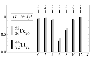
Figure 3: Overlaps of the yrast eigenstates in the $(1f_{7/2})^{4}$ system, for angular momentum $J$ and isospin $T=0$, with the $B$-pair state $|B^{2};J\rangle$. The shell-model interaction is defined in Eq. (39). Also shown are the numbers of $(1f_{7/2})^{4}$ states (top) and of $B$-pair states (bottom) with angular momentum $J$ and isospin $T=0$.

For two neutrons and two protons (both particle- or hole-like) the $B$-pair state is unique for a given total angular momentum $J$ and isospin $T=0$. The $B$-pair content of a given shell-model state can be obtained from Eq. (12) with $\omega=1$. This quantity is shown in Fig. 3 for the yrast states in ⁴⁴Ti and ⁵²Fe. Most yrast states have a large $B$-pair content but not for $J=6$ and $J=8$. It seems as if the two $B$ pairs do not like to couple to a total angular momentum which equals their individual spins. Although the interaction varies considerably with mass (see Table 7.2), similar results are found in ⁴⁴Ti and ⁵²Fe, indicating that these conclusions are robust as long as a reasonable nuclear interaction is used.

Also shown in Fig. 3 are the numbers of $(1f_{7/2})^{4}$ states and of $B$-pair states with angular momentum $J$ and isospin $T=0$. This allows one to judge whether the observation of a high overlap is trivial or meaningful. For example, only one shell-model state exists with $J=12$ and $T=0$ which therefore necessarily has an overlap of 1 with the $B$-pair state. In contrast, four shell-model states exist with $J=2$ and $T=0$ but it is found that the yrast eigenstate has an overlap of more than 0.98 with a single $B$-pair state. The latter is a physically meaningful result whereas the former is trivial.

Figure 4: The yrast spectrum of ⁴⁴Ti. Levels are labelled by their angular momentum and parity $J^{\pi}$. The different columns contain the experimental [42] levels (Expt), the results of the $(1f_{7/2})^{4}$ shell model (SM) with the interaction (39), the expectation value of the shell-model hamiltonian in the $B$-pair state ($B^{2}$) and the expectation value of the mapped boson hamiltonian with up to two-body interactions ($b^{2}[2]$). The shell-model energy of the $0^{+}_{1}$ level is normalized to zero.

Figure 5: Same as Fig. 4 for ⁵²Fe.

The energy spectra of ⁴⁴Ti and ⁵²Fe, shown in Figs. 4 and 5, confirm the above wave-function analysis. For the sake of comparison with the data, the shell-model energy of the $0^{+}$ level is normalized to zero, and it is seen that the excitation spectra calculated in the shell model (SM) are reasonably close to the observed ones. The column ‘$B^{2}$’ shows the expectation value of the shell-model hamiltonian in the $B$-pair state $|B^{2};J,T=0\rangle$. Note that absolute energies are calculated which are plotted relative to the shell-model $0^{+}_{1}$ level. Therefore, the differences in energy between corresponding levels in the ‘SM’ and ‘$B^{2}$’ columns correlate with the overlaps shown in Fig. 3. For example, the difference is greatest for $J^{\pi}=6^{+}$ since for this state the overlap is smallest.

Coefficients $a^{L}_{JT}(j)$ in the expansion (40) for $j=7/2$. $L$ 0 2 4 6 8 10 12 $(JT)$ $(01)$ $\frac{19305}{13732}$ $\phantom{-}\frac{1287}{1312}$ $\frac{3315}{8612}$ $\frac{14535}{245288}$ $(10)$ $\frac{35035}{41196}$ $\phantom{-}\frac{2821}{3936}$ $\frac{11305}{25836}$ $\frac{110789}{735864}$ $\frac{38}{2913}$ $(21)$ $\frac{21021}{13732}$ $\phantom{-}\frac{2379}{1312}$ $\frac{16711}{8612}$ $\frac{332367}{245288}$ $\frac{399}{971}$ $(30)$ $\frac{22295}{151052}$ $\phantom{-}\frac{3969}{14432}$ $\frac{145775}{284196}$ $\frac{1779141}{2698168}$ $\frac{5047}{10681}$ $\frac{115}{1221}$ $(41)$ $\frac{9555}{151052}$ $\phantom{-}\frac{2949}{14432}$ $\frac{62475}{94732}$ $\frac{4007955}{2698168}$ $\frac{45465}{21362}$ $\frac{2415}{1628}$ $(50)$ $\frac{245}{178516}$ $\phantom{-}\frac{147}{17056}$ $\frac{16415}{335868}$ $\frac{46305}{245288}$ $\frac{12515}{25246}$ $\frac{4711}{5772}$ $\frac{6}{13}$ $(61)$ $\frac{15}{151052}$ $\phantom{-}\frac{21}{14432}$ $\frac{1435}{94732}$ $\frac{270627}{2698168}$ $\frac{9843}{21362}$ $\frac{2469}{1628}$ $3$ $(70)$ $\frac{1}{1716}$ $-\frac{197}{562848}$ $\frac{2293}{3694548}$ $\frac{10337}{8094504}$ $\frac{15589}{833118}$ $\frac{1897}{21164}$ $\frac{7}{13}$

Boson interaction matrix elements $\upsilon^{2\rm b}_{L}$ (in MeV) appropriate for the $1f_{7/2}$ and $1g_{9/2}$ shells. $L$ 0 2 4 6 8 10 12 14 16 18 ⁴²Sc $-3.187$ $-2.576$ $-1.601$ $-1.697$ $-0.372$ $-1.677$ $0.055$ $+\infty$ ⁵⁴Co $-2.551$ $-1.614$ $-1.105$ $-0.730$ $0.101$ $-0.664$ $0.349$ $+\infty$ SLGT0 $-5.635$ $-4.956$ $-3.694$ $-2.333$ $-1.209$ $-0.455$ $-0.062$ $0.058$ $-0.506$ $+\infty$

The two-boson calculation with up to two-body interactions, shown in the column ‘$b^{2}[2]$’ of Fig. 3, reproduces exactly the $B$-pair calculation, in agreement with the discussion of Sect. 5. Since, for a given angular momentum $J$ and isospin $T=0$, the mapping from two $B$ pairs to two $b$ bosons is one-to-one, simple expressions are found for the boson interaction matrix elements $\upsilon^{2\rm b}_{L}$ in terms of the two-body fermion matrix elements $\upsilon^{2\rm f}_{JT}$. These relations are of the generic form

$$\upsilon^{2\rm b}_{L}=\sum_{JT}a^{L}_{JT}(j)\upsilon^{2\rm f}_{JT},$$ (40)

with coefficients $a^{L}_{JT}(j)$ that depend on the single-particle angular momentum $j$ of the shell. The coefficients for $j=7/2$ are given in Table 7.2.1 and the resulting boson interaction matrix elements $\upsilon^{2\rm b}_{L}$ in Table 7.2.1. There is no four-particle shell-model state with $J=14$, implying the choice $\upsilon^{2\rm b}_{14}=+\infty$, in line with the recipe (22). In numerical calculations a large repulsive matrix element is taken.

No three-body interactions between the bosons intervene in ⁴⁴Ti and ⁵²Fe.

7.2.2 ⁴⁶V and ⁵⁰Mn

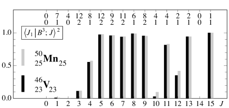
Figure 6: The square of the projection of the yrast eigenstates in the $(1f_{7/2})^{6}$ system onto the subspace spanned by the $B$-pair states $|B^{3};J\rangle$, for angular momentum $J$ and isospin $T=0$. The shell-model interaction is defined in Eq. (39). Also shown are the numbers of $(1f_{7/2})^{6}$ states (top) and of $B$-pair states (bottom) with angular momentum $J$ and isospin $T=0$.

Odd–odd $N=Z$ nuclei are of particular interest with regard to the question of the relevance of neutron–proton pairs. For three neutrons and three protons (both particle- or hole-like) in a $j=7/2$ shell, there are at most two linearly independent $B$-pair states for a given total angular momentum $J$ and isospin $T=0$. The $B$-pair content of a shell-model state can therefore be obtained from Eq. (12) with $\omega=1$ or 2. This quantity is shown in Fig. 6 for yrast states in ⁴⁶V and ⁵⁰Mn. On top of the figure are shown the numbers of $(1f_{7/2})^{6}$ states and of $B$-pair states with angular momentum $J$ and isospin $T=0$, in order to judge whether a large overlap is a physically meaningful or a trivial result.

A surprising feature of the results of Fig. 6 is the ‘schizophrenic’ behaviour of $T=0$ states in ⁴⁶V and ⁵⁰Mn, with most having either a large or a small $B$-pair component. Clearly, only the former states can be interpreted in terms of $B$ pairs or $b$ bosons, as will be shown below. Before doing so, a few words are in order about those states that do not conform to such a description. The most obvious example is the $J=2$ state which simply cannot be constructed out of three $B$ pairs. A wave-function analysis with the method outlined in Sect. 4, gives $|SPD;2\rangle$ as its main component, $\langle 2^{+}_{1}|SPD;2\rangle^{2}=0.825~{}(0.841)$ in ⁴⁶V (⁵⁰Mn), where $S$, $P$ and $D$ are pairs with $J=0,T=1$, $J=1,T=0$ and $J=2,T=1$, respectively. All low-spin states can in fact be adequately written in terms of the $S$, $P$, $D$ and $F$ pairs that correspond to the bosons of IBM-4, confirming the analysis of Juillet et al. [23] in a different mass region. The most remarkable state of this kind is the yrast $1^{+}$ level which approximately can be written as $|P^{3};1\rangle$ since $\langle 1^{+}_{1}|P^{3};1\rangle^{2}=0.725~{}(0.728)$ in ⁴⁶V (⁵⁰Mn). (Note that there is only one $P^{3}$ state with angular momentum $J=1$ since $|P^{3}[0]1\rangle\propto|P^{3}[2]1\rangle$.)

Figure 7: The spectrum of yrast states in ⁴⁶V with isospin $T=0$. Levels are labelled by their angular momentum and parity $J^{\pi}$. The different columns contain the experimental [42] levels (Expt), the results of the $(1f_{7/2})^{6}$ shell model (SM) with the interaction (39), the lowest eigenvalue of the shell-model hamiltonian in the $B$-pair subspace ($B^{3}$) and the lowest eigenvalue of the mapped boson hamiltonian with up to two-body ($b^{3}[2]$) and up to three-body ($b^{3}[3]$) interactions. The shell-model energy of the $T=0$ ground state, $J^{\pi}=3^{+}$, is normalized to the experimental excitation energy of this level which is relative to the $0^{+}$ ground state with isospin $T=1$.

Figure 8: Same as Fig. 7 for ⁵⁰Mn. The shell-model energy of the $T=0$ ground state, $J^{\pi}=5^{+}$, is normalized to the experimental excitation energy of this level which is relative to the $0^{+}$ ground state with isospin $T=1$.

The results of the wave-function analysis are confirmed by the energy spectra shown in Figs. 7 and 8. The observed spectra are reasonably well reproduced in the shell-model calculation, the main deficiency of the latter being that it cannot account for the $3^{+}$–$5^{+}$ inversion of $T=0$ ground states between ⁴⁶V and ⁵⁰Mn. The same level of agreement is found in the $B$-pair calculation except that the low-spin states ($1^{+}$, $2^{+}$, $3^{+}$ and $4^{+}$) are at much higher energies (or absent in the case of the $2^{+}$ level), in disagreement with the data.

The mapped two-body boson hamiltonian (column ‘$b^{3}[2]$’) closely reproduces the $B^{3}$ calculation, including its deficient low-spin levels. Consequently, the three-body components of the interaction between the $b$ bosons are small. Let us consider two examples to illustrate the calculation of three-body interactions between the bosons, namely those pertaining to the $5^{+}$ and $7^{+}$ states. Numerical values are quoted for ⁴⁶V, the results obtained for ⁵⁰Mn being similar. For $J=5$ there are two independent fermionic $B^{3}$ states and the diagonalization of the shell-model hamiltonian in this basis yields the eigenvalues $\{E_{k}\}=\{-20.599,-18.456\}$, in MeV. The same number of independent bosonic $b^{3}$ states exists, which can be chosen as $|b^{3}[\tilde{L}_{2}]5\rangle$ with $\tilde{L}_{2}=12$ and 2. The first state in this basis is taken as $\tilde{L}_{2}=12$ because its fermionic analogue, $|B^{3}[\tilde{12}]5\rangle$, has maximum overlap with the shell-model $5^{+}_{1}$ state. The second state in the boson basis is orthogonal to $|b^{3}[\tilde{12}]5\rangle$ and therefore unique, and hence its $\tilde{L}_{2}$ can be chosen freely. The diagonalization of the mapped one-plus-two-body boson hamiltonian in this basis leads to the eigenvalues $\{E^{\prime}_{k}\}=\{-20.897,-18.391\}$, in MeV. The transformation (28) of the differences $\{E_{k}-E^{\prime}_{k}\}=\{0.298,-0.065\}$ back to the orthogonal boson basis leads to the three-body interaction (in MeV)

$$\langle b^{3}[\tilde{L}_{2}]5|\hat{H}^{\rm b}_{3}|b^{3}[\tilde{L}^{\prime}_{2}]5\rangle=\left[\begin{array}[]{rcr}0.290&&0.053\\ 0.053&&-0.057\end{array}\right],\qquad L_{2},L^{\prime}_{2}=12,2.$$ (41)

The $J=7$ interaction can be dealt with in a similar way. There are two independent fermionic $B^{3}$ states and the diagonalization of the shell-model hamiltonian in the $B$-pair space leads to the eigenvalues $\{E_{k}\}=\{-19.639,-16.905\}$, in MeV. In this case there are three independent bosonic states $|b^{3}[\tilde{L}_{2}]7\rangle$ and the choice $\tilde{L}_{2}=0$, 12 and 2 maximizes the overlap with the shell-model $7^{+}_{1}$ state. The diagonalization of the one-plus-two-body boson hamiltonian in this basis yields the eigenvalues $\{E^{\prime}_{k}\}=\{-19.673,-16.925,+\infty\}$, in MeV. The spurious state in the three-boson system is thus removed by the two-body interaction matrix element $\upsilon^{2\rm b}_{14}=+\infty$. Nevertheless, the entire $3\times 3$ matrix must be used to define the three-body interaction for $J=7$. This is achieved by transforming the differences $\{E_{k}-E^{\prime}_{k}\}=\{0.034,-0.020,0.000\}$ back to the orthogonal boson basis, leading to the three-body interaction (in MeV)

$$\langle b^{3}[\tilde{L}_{2}]7|\hat{H}^{\rm b}_{3}|b^{3}[\tilde{L}^{\prime}_{2}]7\rangle=\left[\begin{array}[]{rcrcr}0.019&{}\hfil&0.014&&-0.010\\ 0.014&&0.020&&0.003\\ -0.010&&0.003&&0.017\end{array}\right],\qquad L_{2},L^{\prime}_{2}=0,12,2.$$ (42)

Typically, the three-body matrix elements are of the order of a few tens of keV, the matrix element $\langle b^{3}[\tilde{12}]5|\hat{H}^{\rm b}_{3}|b^{3}[\tilde{12}]5\rangle$ in Eq. (41) being by far the largest three-body correction in the $1f_{7/2}$ shell.

It will not have escaped the attention of the diligent reader that the dimensions of all hamiltonian matrices in the different approximations are small. The largest dimension, in the shell-model calculation for six nucleons with $J=3$ or 5 and $T=0$, is twelve. Modern shell-model codes usually adopt an $m$-scheme basis without good angular momentum and isospin but, even so, dimensions in a single-$j$ shell do remain modest, of the order of a few hundred at most. Why then, this diligent reader might well ask, bother to seek a further reduction of dimension in terms of $B$ pairs which introduces major computational complications? The answer is that conceptual insight is gained.

Let us illustrate this with the example of the yrast $5^{+}$ state in ⁴⁶V or ⁵⁰Mn. According to Fig. 6 this state has a large component in the $B$-pair space which is of dimension two. In fact, the analysis of its wave function shows that $\langle 5^{+}_{1}|B^{3}[12]5\rangle^{2}=0.961~{}(0.967)$ in ⁴⁶V (⁵⁰Mn). The $5^{+}_{1}$ state can therefore be written approximately as $|B^{3}[12]5\rangle$, which is nothing but the normalized $B$-pair state (1) with $n=3$, $L_{2}=12$ and $L_{3}=5$, and the structure of this state is now understood in simple terms. For example, within this approximation its energy can be given as

$$E(B^{3}[12]5) = \frac{7695}{11668}\upsilon^{2\rm f}_{01}+\frac{564181}{665076}\upsilon^{2\rm f}_{10}+\frac{6112703}{1551844}\upsilon^{2\rm f}_{21}+\frac{2544169}{2438612}\upsilon^{2\rm f}_{30}+$$ (43)

$$\frac{5814660}{4267571}\upsilon^{2\rm f}_{41}+\frac{3323}{5834}\upsilon^{2\rm f}_{50}+\frac{3705457}{1219306}\upsilon^{2\rm f}_{61}+\frac{340651}{96261}\upsilon^{2\rm f}_{70},$$

in terms of the shell-model two-body matrix elements $\upsilon^{2\rm f}_{JT}$. One notes the large coefficient in front of the ‘quadrupole pairing’ matrix element $\upsilon^{2\rm f}_{21}$. Quadrupole collectivity will therefore strongly influence the energy of the $5^{+}_{1}$ level, in both ⁴⁶V and ⁵⁰Mn.

The derivation of the energy formula (43) is non-trivial since it requires a symbolic implementation of Chen’s recursive algorithm [32], and overlaps involving up to four pairs are needed [see Eq. (15)]. On the basis of more ‘elementary’ techniques, an approximate formula can be obtained as follows. For a three-boson state, its diagonal energy originating from a two-body interaction can be written with CFPs,

$$V(b^{3}[L_{2}]L_{3})=3\sum_{L^{\prime}_{2}}[\ell^{2}(L^{\prime}_{2})\ell|\}\ell^{3}[L_{2}]L_{3}]^{2}\upsilon^{2\rm b}_{L^{\prime}_{2}},$$ (44)

which are know in closed form in terms of Racah coefficients [40], leading to the expression

$$V(b^{3}[12]5) = \frac{4370}{11557}\upsilon^{2\rm b}_{2}+\frac{512325}{392938}\upsilon^{2\rm b}_{4}+\frac{12650}{41021}\upsilon^{2\rm b}_{6}+\frac{300}{31369}\upsilon^{2\rm b}_{8}+$$ (45)

$$\frac{405}{12265279}\upsilon^{2\rm b}_{10}+\frac{14859}{14858}\upsilon^{2\rm b}_{12}.$$

Since the boson interaction matrix elements $\upsilon^{2\rm b}_{L}$ are known in terms of the two-body fermion matrix elements $\upsilon^{2\rm f}_{JT}$ from Eq. (40), the following total energy (which includes the single-boson energy $3\epsilon_{b}$) is found:

$$E(b^{3}[12]5) = 3\epsilon_{b}+V(b^{3}[12]5)$$ (46)

$$= 0.891\,\upsilon^{2\rm f}_{01}+0.888\,\upsilon^{2\rm f}_{10}+3.637\,\upsilon^{2\rm f}_{21}+0.981\,\upsilon^{2\rm f}_{30}+$$

$$1.416\,\upsilon^{2\rm f}_{41}+0.592\,\upsilon^{2\rm f}_{50}+3.056\,\upsilon^{2\rm f}_{61}+3.540\,\upsilon^{2\rm f}_{70},$$

where the coefficients are rational numbers involving very large integers, to which a numerical approximation is given.

Equation (46) is the boson analogue of the shell-model result (43). The expressions are similar but not identical, and this is due to the two-body approximation in the boson calculation. It should be emphasized once more that, if three-body interactions between the bosons are included, results in the $B^{3}$ and $b^{3}$ spaces become identical.

The nuclei ⁴⁶V and ⁵⁰Mn have several isomeric states [42], with half-lives ranging from minutes (the $5^{+}_{1}$ level in ⁵⁰Mn) to milli- and nano-seconds (the $3^{+}_{1}$ and $5^{+}_{1},7^{+}_{1}$ levels in ⁴⁶V, respectively), some of which have known dipole and/or quadrupole moments. The measured magnetic dipole moments can be compared with the simple single-$j$ shell prediction that the $g$ factor of any state in an $N=Z$ nucleus equals $(g_{\nu}+g_{\pi})/2$ (see Subsect. 7.1). The effect of the quenching of the spin part of the M1 operator is small: without quenching $(g_{\nu}+g_{\pi})/2$ equals 0.55 $\mu_{\rm N}$ in the $1f_{7/2}$ shell and, with a quenching of 0.7, it reduces to 0.52 $\mu_{\rm N}$. Therefore, the single-$j$ shell model predicts magnetic dipole moments $\mu(J^{\pi})$ of states in $N=Z$ nuclei in the $1f_{7/2}$ shell of the order of $0.52J$ to $0.55J$ $\mu_{\rm N}$. This agrees with the measured [45, 46] values of $\mu(3^{+}_{1})=1.64~{}(3)$ $\mu_{\rm N}$ in ⁴⁶V and $\mu(5^{+}_{1})=2.76~{}(1)$ $\mu_{\rm N}$ in ⁵⁰Mn. As argued in Subsect. 7.1, this result does not constitute a test of the $B$-pair or $b$-boson approximation, but shows consistency with a single-$j$ shell truncation. The large-scale shell-model result with the gxpf1a interaction [46], $\mu(5^{+}_{1})=2.81$ $\mu_{\rm N}$, also agrees with the data.

Charlwood et al. [46] also measured the quadrupole moment of the $5^{+}$ isomer in ⁵⁰Mn, $Q(5^{+}_{1})=+0.80~{}(12)$ b. In the large-scale shell model with the gxpf1a interaction [46] one finds a smaller value of $Q(5^{+}_{1})=+0.58$ b. A numerical calculation in a single-$j$ shell gives $Q(5^{+}_{1})=+4.2(e_{\nu}+e_{\pi})l_{\rm ho}^{2}$, in terms of the neutron (proton) effective charges $e_{\nu}$ ($e_{\pi}$) and the oscillator length $l_{\rm ho}$ of Eq. (34). This shell-model result can be compared with the approximation in terms of $b$ bosons that assumes $|5^{+}_{1}\rangle\approx|b^{3}[12]5\rangle$. One uses the definition

$$Q(b^{3}[L_{2}]L_{3})=\sqrt{\frac{16\pi}{5}}\left(\begin{array}[]{rcrcr}L_{3}&{}\hfil&2&{}\hfil&L_{3}\\ -L_{3}&&0&&L_{3}\end{array}\right)\langle b^{3}[L_{2}]L_{3}||e_{b}(b^{\dagger}\times\tilde{b})^{(2)}||b^{3}[L_{2}]L_{3}\rangle,$$ (47)

where the reduced matrix element is obtained from

$$\langle b^{3}[L_{2}]L_{3}||(b^{\dagger}\times\tilde{b})^{(\lambda)}||b^{3}[L^{\prime}_{2}]L^{\prime}_{3}\rangle=3(-)^{\ell+L_{3}+\lambda}\sqrt{(2\lambda+1)(2L_{3}+1)(2L^{\prime}_{3}+1)}$$ (50)

$$\qquad\qquad\times\sum_{L^{\prime\prime}_{2}}[\ell^{2}(L^{\prime\prime}_{2})\ell|\}\ell^{3}[L_{2}]L_{3}][\ell^{2}(L^{\prime\prime}_{2})\ell|\}\ell^{3}[L^{\prime}_{2}]L^{\prime}_{3}]\left\{\begin{array}[]{ccccc}\ell&{}\hfil&L_{3}&{}\hfil&L^{\prime\prime}_{2}\\ L^{\prime}_{3}&&\ell&&\lambda\end{array}\right\}.$$

For $L_{2}=12$ and $L_{3}=5$ and with the effective boson charge taken from Eq. (38), one finds

$$Q(b^{3}[12]5)=-\frac{649485}{150241}(e_{\nu}+e_{\pi})l_{\rm ho}^{2}\approx-4.3(e_{\nu}+e_{\pi})l_{\rm ho}^{2},$$ (51)

in excellent agreement with the single-$j$ shell result, considering that a change of sign of the quadrupole moment is needed to pass from particles to holes [44].

In a single-$j$ shell calculation the quadrupole deformation is significantly underestimated if standard values for the effective charges ($e_{\nu}=0.5$ and $e_{\pi}=1.5$) are taken. The dependence of the quadrupole moments on effective charges and on the oscillator length can be eliminated by considering ratios. For example, by making the associations $|7^{+}_{1}\rangle=|b\rangle$ and $|5^{+}_{1}\rangle\approx|b^{3}[12]5\rangle$ for the $7^{+}_{1}$ and $5^{+}_{1}$ states in ⁴²Sc and ⁴⁶V, respectively, one obtains the ratio

$$\frac{Q(5^{+}_{1};\,^{46}{\rm V})}{Q(7^{+}_{1};\,^{42}{\rm Sc})}\approx\frac{Q(b^{3}[12]5)}{Q(b)}=\frac{216495}{150241}\approx 1.44.$$ (52)

This is a parameter-independent test of the validity of the $b$-boson approximation.

7.2.3 ⁴⁸Cr

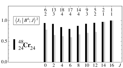
Figure 9: The square of the projection of the yrast eigenstates in the $(1f_{7/2})^{8}$ system onto the subspace spanned by the $B$-pair states $|B^{4};J\rangle$, for angular momentum $J$ and isospin $T=0$. The shell-model interaction is defined in Eq. (39). Also shown are the numbers of $(1f_{7/2})^{8}$ states (top) and of $B$-pair states (bottom) with angular momentum $J$ and isospin $T=0$. The grey bars represent the corresponding analysis in terms of the stretched configuration of Danos and Gillet [28, 29] (see text).

Figure 10: The yrast spectrum of ⁴⁸Cr. Levels are labelled by their angular momentum and parity $J^{\pi}$. The different columns contain the experimental [42] levels (Expt), the results of the $(1f_{7/2})^{8}$ shell model (SM) with the interaction (39), the lowest eigenvalue of the shell-model hamiltonian in the $B$-pair subspace ($B^{4}$) and the lowest eigenvalue of the mapped boson hamiltonian with up to two-body ($b^{3}[2]$) and up to three-body ($b^{3}[3]$) interactions. The shell-model energy of the $0^{+}_{1}$ level is normalized to zero.

The $B$-pair content of yrast states in ⁴⁸Cr is displayed in Fig. 9 while its energy spectrum, calculated in various approximations, single-$j$ shell model (SM), shell-model $B$-pair approximation ($B^{4}$) and mapped $b$-boson calculation with up to two-body ($b^{4}[2]$) and three-body ($b^{4}[3]$) interactions, is shown in Fig. 10.

Two issues of interest arise for the eight-nucleon system. First, it is possible to establish an explicit connection with the stretch scheme of Danos and Gillet [28, 29], since their eight-nucleon stretched state $|B^{4}_{\rm s}J\rangle$ with angular momentum $J$ can in fact be written as

$$|B^{4}_{\rm s}J\rangle \propto \left(\left(B^{\dagger}\times B^{\dagger}\right)^{(J_{\rm max})}\times\left(B^{\dagger}\times B^{\dagger}\right)^{(J_{\rm max})}\right)^{(J)}|{\rm o}\rangle$$ (55)

$$= (-)^{J}\sum_{L}\sqrt{(2J_{\rm max}+1)(2L+1)}\left\{\begin{array}[]{ccccc}J_{\rm max}&&\ell&&L\\ \ell&&J&&J_{\rm max}\end{array}\right\}|B^{4}J_{\rm max}LJ\rangle,$$

in terms of the $B$-pair states (1) with $J_{\rm max}=4j-2$. It is therefore possible to determine the ‘stretch’ content of a shell-model state since it can be done for the states on the right-hand side of Eq. (55) with the formalism developed in Sect. 4. Note that, unlike in the original discussion of Danos and Gillet [28, 29], anti-symmetry of the stretched configuration is fully taken into account here. The stretch content of yrast states in ⁴⁸Cr is shown with grey bars in Fig. 9. It is clear from Eq. (55) that the stretched configuration is but one particular vector in the $B$-pair space and the stretch content of any state is therefore necessary smaller than its $B$-pair content. If the dimension of the $B$-pair space reduces to one, as is the case for $J=14$ and 16, both approximations become identical. These findings are completely at variance with the results of Daley [30].

The second question of interest concerns the formation of a $B$-pair condensate. The ground state lies dominantly in the $B$-pair space and can, to a good approximation, be written in terms of a single component $|B^{2}[0]B^{2}[0];0\rangle$ which arises by the coupling of pairs of $B$ pairs to angular momentum zero. A wave-function analysis shows that $\langle 0^{+}_{1}|B^{2}[0]B^{2}[0];0\rangle^{2}=0.927$, close to full $B$-pair content of 0.940. A similar approximation is possible for the $2^{+}_{1}$ state for which $\langle 2^{+}_{1}|B^{2}[0]B^{2}[2];2\rangle^{2}=0.918$. In view of these large overlaps, it is then tempting to postulate a seniority-like scheme for the $B$ pairs [and therefore an SO($2\ell+1$) classification for the $b$ bosons] but this would be wrong. Although the $4^{+}_{1}$ state has a dominant $B$-pair content (84.2%), its $B$-pair seniority-like component is negligible, $\langle 4^{+}_{1}|B^{2}[0]B^{2}[4];4\rangle^{2}=0.005$. The two-body boson interactions, derived from the shell model and shown in Table 7.2.1, do not allow an obvious treatment in terms of boson symmetries. It remains nevertheless true that the single component $|B^{2}[0]B^{2}[0];0\rangle$ provides a good approximation to the ground state of the eight-nucleon system. It would be of some interest to generalize this finding to larger single-$j$ shells and to many particles.

7.3 The $1g_{9/2}$ shell

Nuclei in the $1g_{9/2}$ shell were the focus of a previous study [48], with a wave-function analysis limited to $n=4$ and boson interactions limited to two-body. Additional material and further details of the calculations are presented in the subsequent subsections. The shell-model interaction, referred to as SLGT0, is taken from Serduke et al. [49] and gives satisfactory results for the neutron-deficient nuclei in the mass region $A=86$ to 100 [50]. Being defined in the $2p_{1/2}+1g_{9/2}$ shell-model space, this interaction is renormalized to the $1g_{9/2}$ orbit. The resulting matrix elements are given in Table 7.2.

7.3.1 ⁹⁶Cd

Figure 11: Overlaps of the yrast eigenstates in the $(1g_{9/2})^{4}$ system, for angular momentum $J$ and isospin $T=0$, with the $B$-pair state $|B^{2};J\rangle$. The shell-model interaction SLGT0 is defined in Table 7.2. Also shown are the numbers of $(1g_{9/2})^{4}$ states (top) and of $B$-pair states (bottom) with angular momentum $J$ and isospin $T=0$.

The study of this nucleus is at the limit of present experimental capabilities. A fusion–evaporation experiment was proposed at GANIL some time ago [51] but had to be rescheduled to due to technical difficulties. In view of this current interest, it is worthwhile to investigate the $B$-pair structure of ⁹⁶Cd. The $B$-pair content of shell-model states calculated with the SLGT0 interaction is shown in Fig. 11. Results are entirely consistent with those obtained in the $1f_{7/2}$ shell (see Fig. 3), indicating the generic nature of the analysis, independent of the particular value of $j$ of the shell considered. The decrease of the $B$-pair content at intermediate values of the angular momentum $J$ can be understood on the basis of a combination of geometry—the CFPs in a single-$j$ shell, and dynamics—the dependence of the interaction matrix elements on $J$ and $T$ [48].

Figure 12: The yrast spectrum of ⁹⁶Cd. Levels are labelled by their angular momentum and parity $J^{\pi}$. No experimental levels are known to date. The different columns contain the results of the $(1g_{9/2})^{4}$ shell model (SM) with the SLGT0 interaction, the expectation value of the shell-model hamiltonian in the $B$-pair state ($B^{2}$) and the expectation value of the mapped boson hamiltonian with up to two-body interactions ($b^{2}[2]$). The shell-model energy of the $0^{+}_{1}$ level is normalized to zero.

Coefficients $a^{L}_{JT}(j)$ in the expansion (40) for $j=9/2$. $L$ 0 2 4 6 8 10 12 14 16 $(JT)$ $(01)$ $\frac{4862}{4265}$ $\phantom{-}\frac{117572}{137755}$ $\frac{2261}{5445}$ $\phantom{-}\frac{7429}{65120}$ $\frac{1311}{110210}$ $(10)$ $\frac{35802}{46915}$ $\phantom{-}\frac{976752}{1515305}$ $\frac{2261}{5445}$ $\phantom{-}\frac{11799}{65120}$ $\frac{50301}{1212310}$ $\frac{345}{156739}$ $(21)$ $\frac{15912}{9383}$ $\phantom{-}\frac{543932}{303061}$ $\frac{13889}{7986}$ $\phantom{-}\frac{45011}{35816}$ $\frac{67068}{121231}$ $\frac{15525}{156739}$ $(30)$ $\frac{139944}{609895}$ $\phantom{-}\frac{6520724}{19698965}$ $\frac{771799}{1557270}$ $\phantom{-}\frac{165669}{291005}$ $\frac{3425436}{7880015}$ $\frac{359415}{2037607}$ $\frac{1218}{69355}$ $(41)$ $\frac{99144}{609895}$ $\phantom{-}\frac{6750054}{19698965}$ $\frac{618032}{778635}$ $\phantom{-}\frac{821583}{582010}$ $\frac{13883076}{7880015}$ $\frac{2774250}{2037607}$ $\frac{63423}{138710}$ $(50)$ $\frac{408}{55445}$ $\phantom{-}\frac{43358}{1790815}$ $\frac{686}{7865}$ $\phantom{-}\frac{483}{2035}$ $\frac{334476}{716365}$ $\frac{578322}{926185}$ $\frac{29957}{63050}$ $\frac{868}{8515}$ $(61)$ $\frac{153}{93830}$ $\phantom{-}\frac{13699}{1515305}$ $\frac{343}{6655}$ $\phantom{-}\frac{76797}{358160}$ $\frac{789021}{1212310}$ $\frac{1113966}{783695}$ $\frac{109881}{53350}$ $\frac{1953}{1310}$ $(70)$ $\frac{81}{4147286}$ $\phantom{-}\frac{13608}{66976481}$ $\frac{1673}{882453}$ $\phantom{-}\frac{14823}{1217744}$ $\frac{3024621}{53584102}$ $\frac{6727847}{34639319}$ $\frac{1148337}{2358070}$ $\frac{46251}{57902}$ $\frac{8}{17}$ $(81)$ $\frac{1}{1219790}$ $\phantom{-}\frac{378}{19698965}$ $\frac{161}{519090}$ $\phantom{-}\frac{29223}{9312160}$ $\frac{175176}{7880015}$ $\frac{1202172}{10188035}$ $\frac{15231}{31525}$ $\frac{1977}{1310}$ 3 $(90)$ $\frac{1}{24310}$ $-\frac{8081}{334882405}$ $\frac{23}{802230}$ $-\frac{101}{14391520}$ $\frac{61018}{133960255}$ $\frac{479646}{173196595}$ $\frac{10893}{535925}$ $\frac{2211}{22270}$ $\frac{9}{17}$

The energy spectrum of ⁹⁶Cd, calculated in various approximations, single-$j$ shell model (SM), shell-model $B$-pair approximation ($B^{2}$) and mapped $b$-boson calculation ($b^{2}[2]$), is shown in Fig. 12. Results are seen to be consistent with the wave-function analysis. The boson interaction matrix elements $\upsilon^{2\rm b}_{L}$ are known analytically in terms of the two-body fermion matrix elements $\upsilon^{2\rm f}_{JT}$ [see Eq. (40)] with universal coefficients $a^{L}_{JT}(j=9/2)$ given in Table 7.3.1. The resulting boson interaction matrix elements are shown in Table 7.2.1. There is no four-particle shell-model state with $J=18$, implying the choice $\upsilon^{2\rm b}_{18}=+\infty$.

7.3.2 ⁹⁴Ag

Not much is known experimentally about ⁹⁴Ag except for the presence of two isomers, with tentative assignments $J^{\pi}=7^{+}$ (presumably the lowest $T=0$ state) and $J^{\pi}=21^{+}$, the latter at $6.7~{}(5)$ MeV above the $0^{+}$ ground state [52, 53]. The subsequent discussion is focussed on the structure of these two states.

Figure 13: The square of the projection of the yrast eigenstates in the $(1g_{9/2})^{6}$ system onto the subspace spanned by the $B$-pair states $|B^{3};J\rangle$, for angular momentum $J$ and isospin $T=0$. The shell-model interaction SLGT0 is defined in Table 7.2. Also shown are the numbers of $(1g_{9/2})^{6}$ states (top) and of $B$-pair states (bottom) with angular momentum $J$ and isospin $T=0$.

The $B$-pair content is obtained from Eq. (12) with $\omega$ up to 3, the maximum dimension of the $B$-pair space (for $J=7$ and 9). This quantity is shown in Fig. 13 for yrast states in ⁹⁴Ag, together with the dimensions of the shell-model and $B$-pair spaces. The results are in total accord with those found in the $1f_{7/2}$ shell (see Fig. 6), considering that the replacement $j=7/2\rightarrow 9/2$ leads to an overall increase of the angular momenta involved. It is seen in particular that the overlaps are high for $J=21$ (which is trivial) and for $J=7$ (which is not), making the analysis of these states in terms of $B$ pairs or $b$ bosons meaningful.

Figure 14: The spectrum of yrast states in ⁹⁴Ag with isospin $T=0$. Levels are labelled by their angular momentum and parity $J^{\pi}$. The different columns contain the experimental [52, 53] levels (Expt), the results of the $(1g_{9/2})^{6}$ shell model (SM) with the SLGT0 interaction, the lowest eigenvalue of the shell-model hamiltonian in the $B$-pair subspace ($B^{3}$) and the lowest eigenvalue of the mapped boson hamiltonian with up to two-body ($b^{3}[2]$) and up to three-body ($b^{3}[3]$) interactions. The shell-model energy of the $T=0$ ground state, $J^{\pi}=7^{+}$, is normalized to the experimental excitation energy of this level which is relative to the $0^{+}$ ground state.

The energy spectrum of $T=0$ states in ⁹⁴Ag is shown in Fig. 14. The shell model with the SLGT0 interaction gives the correct $T=0$ ground-state spin, $J=7$, and the energy of the $21^{+}$ isomer comes out reasonably close to the its observed value. The $B$-pair calculation agrees with the shell model but for the low-spin states ($1^{+}$ to $5^{+}$) which are obtained at much higher energies.

In a shell-model description where three neutrons and three protons are placed in the $1g_{9/2}$ orbit, the $J=21$ state is stretched and therefore unique. In this single-$j$ shell approximation, the $21^{+}$ isomer can therefore be written exactly as $|B^{3}[12]21\rangle$, the normalized $B$-pair state (1) with $n=3$, $L_{2}=12$ and $L_{3}=21$. Chen’s algorithm [32] then provides the following energy expression for this state:

$$E(B^{3}[12]21)=\frac{21}{65}\upsilon^{2\rm f}_{50}+\frac{21}{10}\upsilon^{2\rm f}_{61}+\frac{645}{442}\upsilon^{2\rm f}_{70}+\frac{69}{10}\upsilon^{2\rm f}_{81}+\frac{717}{170}\upsilon^{2\rm f}_{90},$$ (56)

in terms of the two-body fermion matrix elements $\upsilon^{2\rm f}_{JT}$. This energy expression can alternatively (and more simply) be derived with standard techniques involving CFPs. Since a six-nucleon state with angular momentum $J_{6}=21$ and isospin $T_{6}=0$ is unique, its energy is given as

$$E(j^{6}J_{6}=21,T_{6}=0)=\sum_{JT}a_{JT}\upsilon^{2\rm f}_{JT},$$ (57)

with the coefficients $a_{JT}$ known in terms of $6\rightarrow 4$ CFPs [40],

$$a_{JT}=15\sum_{\alpha_{4}J_{4}T_{4}}[j^{4}(\alpha_{4}J_{4}T_{4})j^{2}(JT)|\}j^{6}J_{6}=21,T_{6}=0]^{2}.$$ (58)

It can be verified that this alternative derivation also yields the expression (56), which provides a rigorous check on the correctness of the implementation of Chen’s algorithm. It should be emphasized that the derivation using standard CFP techniques is valid only for shell-model states that are unique, such as the $21^{+}$ isomer. If several states can be constructed for a given $J$ and $T$, no such derivation is possible while an expression still can be found from $B$ pairs, as illustrated below for the $7^{+}$ isomer.

In terms of bosons, the $21^{+}$ isomer arises from the coupling of three $b$ bosons with spin $\ell=9$ to total angular momentum $J=21$. It can be shown [54] that two independent boson states exist with $J=21$, one of which must be spurious. Let us consider this case in detail, to illustrate the mechanism by which spurious states can be eliminated analytically. The two independent boson states may be chosen as $|b^{3}[\tilde{12}]21\rangle$ and $|b^{3}[\tilde{14}]21\rangle$, assumed to be normalized and orthogonal. Since the CFPs needed in a three-particle problem are known in terms of Racah coefficients [40], the energy matrix can be shown to have the following elements:

$$\langle b^{3}[\tilde{12}]21|\hat{H}^{\rm b}_{2}|b^{3}[\tilde{12}]21\rangle = 3\epsilon_{b}+\frac{2833}{2697}\upsilon^{2\rm b}_{12}+\frac{44200}{263469}\upsilon^{2\rm b}_{14}+\frac{2782494}{2546867}\upsilon^{2\rm b}_{16}+\frac{60536}{87823}\upsilon^{2\rm b}_{18},$$

$$\langle b^{3}[\tilde{14}]21|\hat{H}^{\rm b}_{2}|b^{3}[\tilde{14}]21\rangle = 3\epsilon_{b}+\frac{3337047}{1932106}\upsilon^{2\rm b}_{14}+\frac{82824}{87823}\upsilon^{2\rm b}_{16}+\frac{20553}{62326}\upsilon^{2\rm b}_{18},$$ (59)

$$\langle b^{3}[\tilde{12}]21|\hat{H}^{\rm b}_{2}|b^{3}[\tilde{14}]21\rangle = \sqrt{\frac{24582912900}{84841672619}}\upsilon^{2\rm b}_{14}-\sqrt{\frac{7946802864}{7712879329}}\upsilon^{2\rm b}_{16}+\sqrt{\frac{20067684}{88284779}}\upsilon^{2\rm b}_{18},$$

where $\epsilon_{b}$ is the energy of the $b$ boson. The stretched boson interaction matrix element $\upsilon^{2\rm b}_{18}$ appears in the diagonal and the off-diagonal matrix elements and, consequently, in the limit $\upsilon^{2\rm b}_{18}\rightarrow+\infty$, one eigenvalue of the $2\times 2$ matrix (59) tends to infinity while the lowest eigenvalue acquires the expression

$$E(b^{3}_{\infty}21)=3\epsilon_{b}+\frac{6851}{20155}\upsilon^{2\rm b}_{12}+\frac{15488}{21545}\upsilon^{2\rm b}_{14}+\frac{1212882}{624805}\upsilon^{2\rm b}_{16},$$ (60)

where the index ‘$\infty$’ serves as a reminder of the limit procedure used to derive the result. The procedure also yields the components of the state,

$$|b^{3}_{\infty}21\rangle=-\sqrt{\frac{637143}{1968935}}|b^{3}[\tilde{12}]21\rangle+\sqrt{\frac{1331792}{1968935}}|b^{3}[\tilde{14}]21\rangle,$$ (61)

of use in the calculation of the quadrupole moment of the $21^{+}$ isomer (see below). Since the $b$-boson energy and the boson interaction are known in terms of the two-body fermion interaction, Eq. (60) can be converted into

$$E(b^{3}_{\infty}21) = \frac{22134}{3707825}\upsilon^{2\rm f}_{30}+\frac{1152549}{7415650}\upsilon^{2\rm f}_{41}+\frac{1347751953}{5740387250}\upsilon^{2\rm f}_{50}+\frac{8606149749}{4857250750}\upsilon^{2\rm f}_{61}+$$ (62)

$$\frac{354940047213}{214690483150}\upsilon^{2\rm f}_{70}+\frac{1561553973}{220784125}\upsilon^{2\rm f}_{81}+\frac{15411107094}{3753330125}\upsilon^{2\rm f}_{90}.$$

This is an approximate expression since it is derived by use of a mapping that includes up to two-body interactions between the bosons. To what extent it is wrong therefore yields an idea about the reliability of the two-body boson mapping. Since the highest allowed angular momentum for two neutrons and two protons in a $j=9/2$ orbit is $J=16$, only matrix elements $\upsilon^{2\rm f}_{JT}$ with $J\geq 5$ can contribute to the energy of the $J=21$ state. This rule is obviously obeyed in Eq. (56) but violated in Eq. (62). It is seen, however, that the coefficients of $\upsilon^{2\rm f}_{30}$ and $\upsilon^{2\rm f}_{41}$ are rather small in the latter expression, indicating that the two-body boson approximation is reasonably accurate.

The perplexed reader might well wonder what could be the purpose of quoting in Eq. (62) the coefficients $a_{JT}$ as the ratio of two ridiculously large integers. The advantage of the use of exact numbers is that enables a rigorous check of fermionic as well as bosonic calculations. The coefficients $a_{JT}$ in an energy expression $E(j^{n}J_{n}T_{n})=\sum_{JT}a_{JT}\upsilon^{2\rm f}_{JT}$ for a unique $n$-particle shell-model state $j^{n}$ with total angular momentum $J_{n}$ and isospin $T_{n}$, satisfy the identities

$$\sum_{JT}a_{JT} = \frac{n(n-1)}{2},$$

$$\sum_{JT}J(J+1)a_{JT} = J_{n}(J_{n}+1)+j(j+1)\times n(n-2),$$

$$\sum_{JT}T(T+1)a_{JT} = T_{n}(T_{n}+1)+{\frac{3}{4}}n(n-2).$$ (63)

These identities reflect the conservation of particle number, angular momentum and isospin in the shell model and are therefore valid for the coefficients in Eq. (56). They are also exactly satisfied by the coefficients in Eq. (62). This is a consequence of the preservation of $n$, $J$ and $T$ under the mapping procedure.

The yrast $7^{+}$ state in ⁹⁴Ag is the analogue of the $5^{+}$ state in ⁴⁶V or ⁵⁰Mn, discussed in Subsect. 7.2.2. Its structure is particularly simple since a wave-function analysis shows that $\langle 7^{+}_{1}|B^{3}[16]7\rangle^{2}=0.908$. The $7^{+}$ isomer is now understood in simple terms as it results from the coupling of two $B$ pairs to maximal angular momentum $J=16$ ($J=18$ is not allowed by the Pauli principle) which is subsequently coupled with the third $B$ pair to total $J=7$. Within this approximation its energy is calculated as

$$E(B^{3}[16]7) = 0.528\upsilon^{2\rm f}_{01}+0.654\upsilon^{2\rm f}_{10}+3.302\upsilon^{2\rm f}_{21}+1.081\upsilon^{2\rm f}_{30}+1.977\upsilon^{2\rm f}_{41}+$$ (64)

$$0.256\upsilon^{2\rm f}_{50}+0.190\upsilon^{2\rm f}_{61}+0.480\upsilon^{2\rm f}_{70}+3.002\upsilon^{2\rm f}_{81}+3.529\upsilon^{2\rm f}_{90}.$$

For the SLGT0 interaction this formula gives an energy of $-11.069$ MeV, to be compared with a correlation energy of $-11.276$ MeV if the full $(1g_{9/2})^{6}$ shell-model basis is used. Note also that the approximate energy expression for the $7^{+}_{1}$ state in the $(1g_{9/2})^{6}$ system is similar to the one obtained in Eq. (43) for the $5^{+}_{1}$ state in the $(1f_{7/2})^{6}$ system.

Since the dimension of the $B$-pair space is three and equals the number of independent states for three $b$ bosons with spin $\ell=9$, no spurious boson states occur for $J=7$. The calculation of the energy of the three-boson state $|b^{3}[16]7\rangle$ in a two-body boson approximation is then straightforward and proceeds along the lines of the energy calculation for the $5^{+}$ state in Subsect. 7.2.2 [see Eqs. (44), (45) and (46)], leading to the expression

$$E(b^{3}[16]7) = 0.711\upsilon^{2\rm f}_{01}+0.711\upsilon^{2\rm f}_{10}+3.118\upsilon^{2\rm f}_{21}+0.997\upsilon^{2\rm f}_{30}+1.933\upsilon^{2\rm f}_{41}+$$ (65)

$$0.278\upsilon^{2\rm f}_{50}+0.235\upsilon^{2\rm f}_{61}+0.484\upsilon^{2\rm f}_{70}+3.004\upsilon^{2\rm f}_{81}+3.529\upsilon^{2\rm f}_{90},$$

in close correspondence with the fermion result (64) that takes into account the exchange terms between the $B$ pairs.

The discussion of Subsect. 7.1 concerning magnetic dipole moments also applies to the $1g_{9/2}$ shell. The single-$j$ shell prediction for the $g$ factor of any state in a $1g_{9/2}$ $N=Z$ nucleus is 0.54 $\mu_{\rm N}$ without spin quenching and 0.51 $\mu_{\rm N}$ with a quenching of 0.7. Magnetic dipole moments do not provide a test of the $B$-pair or $b$-boson approximation but measured $\mu$ values that deviate from the narrow range predicted in a single-$j$ shell, would be indicative of admixtures of configurations beyond the $1g_{9/2}$ shell.

It is also of interest to predict the quadrupole moments of the isomeric states in ⁹⁴Ag. The shell-model calculation in a single-$j$ approximation can be worked analytically for $J=21$ since the state is unique,

$$Q(B^{3}[12]21)=-\sqrt{\frac{196}{6}}(e_{\nu}+e_{\pi})l_{\rm ho}^{2}\approx-0.42~{}{\rm b}.$$ (66)

The corresponding boson result is obtained from the expansion (61), together with the general expressions (47) and (50), leading to

$$Q(b^{3}_{\infty}21)=-\sqrt{\frac{81949367824}{3489855625}}(e_{\nu}+e_{\pi})l_{\rm ho}^{2}\approx-0.44~{}{\rm b},$$ (67)

which illustrates the reliability of the boson approximation. The shell-model value of the quadrupole moment of the $7^{+}$ isomer can be obtained numerically and, in a single-$j$ shell approximation, gives $Q(7^{+}_{1})=+6.60(e_{\nu}+e_{\pi})l_{\rm ho}^{2}\approx+0.60$ b. The dominant component of this state in terms of $b$ bosons is $|b^{3}[16]7\rangle$ for which, from Eqs. (47) and (50), the following quadrupole moment is found:

$$Q(b^{3}[16]7)=-\sqrt{\frac{30930277300923364}{627253477610841}}(e_{\nu}+e_{\pi})l_{\rm ho}^{2}\approx-0.64~{}{\rm b}.$$ (68)

The quadrupole moments (66), (67) and (68) are given for particle–particle configurations; an additional sign is needed to pass to the hole–hole nucleus ⁹⁴Ag.

A final word is needed on the nature of boson approximation. Consider as an example the matrix element

$$\langle B^{3}[4]7|B^{3}[16]7\rangle=\sqrt{\frac{112919600563049280}{139849953265085321}}\approx 0.899,$$ (69)

where it is assumed that bra and ket states are normalized but evidently non-orthogonal. As can be expected from a fraction which involves very large integers, the calculation of this overlap is non-trivial. The corresponding boson result,

$$\langle b^{3}[4]7|b^{3}[16]7\rangle=\sqrt{\frac{7012200}{8733503}}\approx 0.896,$$ (70)

is obtained much more simply in terms of $3\rightarrow 2$ CFPs associated with bosons with spin $\ell=9$. The reliability of the mapping of $B$ pairs onto $b$ bosons ultimately is due to the negligible effect of exchange terms between the $B$ pairs. It cannot be emphasized enough that the calculation of matrix elements of the type (69) is highly non-trivial and quickly runs into computational problems as the number of pairs increases. By comparison, the calculation of overlaps of the type (70) is trivial and can easily be done for all cases of relevance.

7.3.3 ⁹²Pd

The low-lying yrast states of this nucleus were measured by Cederwall et al. [25] with the aim to probe the importance of aligned neutron–proton pairs in $N\sim Z$ nuclei. An analysis of shell-model wave functions in terms of $B$ pairs, as performed for all $N=Z$ nuclei previously considered, becomes tedious in this case, owing to the dimensions of complete bases $|\bar{P}^{n}_{r}\rangle$ in terms of pairs $P^{\dagger}_{\Gamma M_{\Gamma}}$. The complete study of the $1f_{7/2}$ shell presented in Subsect. 7.2 and the results obtained so far for the $1g_{9/2}$ shell indicate that an analysis of ⁹²Pd in the $B$-pair subspace and a subsequent mapping to $b$ bosons should give meaningful results.

Figure 15: The yrast spectrum of ⁹²Pd. Levels are labelled by their angular momentum and parity $J^{\pi}$. The different columns contain the experimental [25] levels (Expt), the results of the $(1g_{9/2})^{8}$ shell model (SM) with the SLGT0 interaction, the lowest eigenvalue of the shell-model hamiltonian in the $B$-pair subspace ($B^{4}$) and the lowest eigenvalue of the mapped boson hamiltonian with up to two-body ($b^{4}[2]$) and up to three-body ($b^{4}[3]$) interactions. The shell-model energy of the $0^{+}_{1}$ level is normalized to zero.

The energy spectrum of ⁹²Pd, calculated in various approximations, single-$j$ shell model (SM), shell-model $B$-pair approximation ($B^{4}$) and mapped $b$-boson calculation with up to two-body ($b^{4}[2]$) and three-body ($b^{4}[3]$) interactions, is shown in Fig. 15. The $B$-pair calculation shows an underbinding of about $0.8$ MeV. This feature is considerably improved if $S$ pairs or $s$ bosons are added to the basis [48].

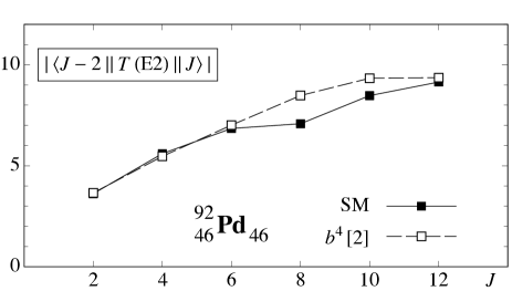
Figure 16: Absolute values of the reduced matrix elements of the E2 operator for the transitions $J\rightarrow J-2$ between yrast states with $T=0$ (⁹²Pd), calculated in the $(1g_{9/2})^{8}$ shell model (SM) with the SLGT0 interaction and compared with the mapped $b$-boson calculation ($b^{4}[2]$). Matrix elements are expressed in units $(e_{\nu}+e_{\pi})l_{\rm ho}^{2}$.

A final illustration of the $b$-boson approximation is provided in Fig. 16 where E2 transition strengths between yrast $(1g_{9/2})^{8}$ states as calculated in the shell model are compared with those obtained with $b$ bosons. The shell-model reduced matrix elements are calculated with the operator (34) and expressed in units $(e_{\nu}+e_{\pi})l_{\rm ho}^{2}$. The reduced matrix elements in the boson approximation are calculated with the operator (36) with an effective boson charge $e_{b}$, determined from the neutron and proton effective charges according to Eq. (37). A small depletion of the shell-model E2 strength is perceptible for $J\approx 8$ and is absent in the boson calculation. Apart from this deviation both calculations agree, indicating once more that the shell-model wave functions can be adequately represented in terms of a single $b$ boson. It should be emphasized that, although the number of $B$-pair states is but a small subset of the total number of possible shell-model states, no effective boson charge is needed to arrive at the agreement found in Fig. 16.

8 Conclusions

What can be concluded with regard to the three approximations enounced in Sect. 6? (i) Can the shell-model space be truncated to a single high-$j$ orbit? (ii) Can the single-$j$ shell space be reduced to one written in terms of aligned $B$ pairs? (iii) And, finally, can the aligned $B$ pair be replaced by a $b$ boson? The answer to the question (iii) is unreservedly positive: owing to its high angular momentum, the $B$ pair behaves much as a boson. The mapping from $B$-pair to $b$-boson space can be made exact by including appropriate interactions between the bosons but becomes approximate if higher-order interactions are neglected. The examples of the $1f_{7/2}$ and $1g_{9/2}$ shells show that two-body interactions between the bosons suffice and that no higher-order interactions are needed. The answer to question (ii) is positive for most but not for all yrast states, that is, most but not all yrast states of $N=Z$ nuclei can be written in terms of $B$ pairs. Odd–odd $N=Z$ nuclei in particular behave in a schizophrenic manner with only a subset of their yrast states having a sizeable $B$-pair content. Other states, mostly of low angular momentum, require the inclusion of low-spin pairs such as those mapped onto the corresponding bosons of the IBM-4. In almost all cases, however, a simple interpretation can be given of yrast states in terms of neutron–proton pairs and this enables one to intuit the complex spectroscopy of odd–odd $N=Z$ nuclei and to derive simple parameter-free predictions. The validity of the truncation to a single-$j$ shell depends on specific features of a realistic shell-model hamiltonian and the answer to question (i) may therefore be different for the $1f_{7/2}$ and $1g_{9/2}$ shells considered in this review. A recent large-scale shell-model calculation with a realistic effective interactions seems to indicate that the truncation to $1g_{9/2}$ (and therefore the $B$-pair approximation) is justified in the $A\sim 90$–100 region [35]. But, in the end, only the experimental verification of the simple predictions derived on the basis of the $b$-boson approximation will be able to tell whether $N=Z$ nuclei exist with sufficiently isolated single-$j$ shells.

References

- [1] D. Brink and R. Broglia, Nuclear Superfluidity: Pairing in Finite Systems (Cambridge University Press, Cambridge, 2005).
- [2] P. Fröbrich, Phys. Lett. B 37 (1971) 388.
- [3] J. Engel, K. Langanke and P. Vogel, Phys. Lett. B 389 (1996) 211.
- [4] P. Vogel, Nucl. Phys. A 662 (2000) 148.
- [5] A.O. Macchiavelli, P. Fallon, R.M. Clark, M. Cromaz, M.A. Deleplanque, R.M. Diamond, G.J. Lane, I.Y. Lee, F.S. Stephens, C.E. Svensson, K. Vetter and D. Ward, Phys. Rev. C 61 (2000) 041303(R).
- [6] R. Chasman, Phys. Lett. B 524 (2002) 81.
- [7] P. Van Isacker, D.D. Warner and A. Frank, Phys. Rev. Lett. 94 (2005) 162502.
- [8] G.F. Bertsch and Y. Luo, Phys. Rev. C 81 (2010) 064320.
- [9] A.O. Macchiavelli, in 50 years of Nuclear BCS: Pairing in Finite Systems, edited by R.A. Broglia and V. Zelevinski (World Scientific, Singapore, 2013).
- [10] A. Arima and F. Iachello, Phys. Rev. Lett. 35 (1975) 1069.
- [11] A. Arima, T. Otsuka, F. Iachello and I. Talmi, Phys. Lett. B 66 (1977) 205.
- [12] J.P. Elliott and A.P. White, Phys. Lett. B 97 (1980) 169.
- [13] M.J. Thompson, J.P. Elliott and J.A. Evans, Phys. Lett. B 195 (1987) 511.
- [14] J.P. Elliott and J.A. Evans, Phys. Lett. B 101 (1981) 216.
- [15] E.P. Wigner, Phys. Rev. 51 (1937) 946.
- [16] P. Halse, J.P. Elliott and J.A. Evans, Nucl. Phys. A 417 (1984) 301.
- [17] P. Halse, Nucl. Phys. A 445 (1985) 93.
- [18] K.T. Hecht and A. Adler, Nucl. Phys. A 137 (1969) 129.
- [19] A. Arima, M. Harvey and K. Shimizu, Phys. Lett. B 30 (1969) 517.
- [20] D. Strottman, Nucl. Phys. A 188 (1972) 488.
- [21] P. Van Isacker, O. Juillet and F. Nowacki, Phys. Rev. Lett. 82 (1999) 2060.
- [22] S.M. Vincent, P.H. Regan, D.D. Warner, R.A. Bark, D. Blumenthal, M.P. Carpenter, C.N. Davids, W. Gelletly, R.V.F. Janssens, C.D. O’Leary, C.J. Lister, J. Simpson, D. Seweryniak, T. Saitoh, J. Schwartz, S. Törmänen, O. Juillet, F. Nowacki and P. Van Isacker, Phys. Lett. B 437 (1998) 264.
- [23] O. Juillet, P. Van Isacker and D.D. Warner, Phys. Rev. C 63 (2001) 054312.
- [24] H.M. David, P.J. Woods, G. Lotay, D. Seweryniak, M. Albers, M. Alcorta, M. Carpenter, C.J. Chiara, T. Davinson, C.M. Deibel, D.T. Doherty, C. Homan, R.V.F. Janssens, T. Lauritsen, A.M. Rogers and S. Zhu, Phys. Lett. B, to be published.
- [25] B. Cederwall, F. Ghazi Moradi, T. Bäck, A. Johnson, J. Blomqvist, E. Clément, G. de France, R. Wadsworth, K. Andgren, K. Lagergren, A. Dijon, G. Jaworski, R. Liotta, C. Qi, B.M. Nyakó, J. Nyberg, M. Palacz, H. Al-Azri, A. Algora, G. de Angelis, A. Ataç, S. Bhattacharyya, T. Brock, J.R. Brown, P. Davies, A. Di Nitto, Zs. Dombrádi, A. Gadea, J. Gál, B. Hadinia, F. Johnston-Theasby, P. Joshi, K. Juhá sz, R. Julin, A. Jungclaus, G. Kalinka, S.O. Kara, A. Khaplanov, J. Kownacki, G. La Rana, S.M. Lenzi, J. Molnár, R. Moro, D.R. Napoli, B.S. Nara Singh, A. Persson, F. Recchia, M. Sandzelius, J.-N. Scheurer, G. Sletten, D. Sohler, P.-A. Söderström, M.J. Taylor, J. Timár, J.J. Valiente-Dobón, E. Vardaci and S. Williams, Nature 469 (2011) 68.
- [26] C. Qi, J. Blomqvist, T. Bäck, B. Cederwall, A. Johnson, R.J. Liotta, and R. Wyss, Phys. Rev. C 84 (2011) 021301(R).
- [27] Z.X. Xu, C. Qi, J. Blomqvist, R.J. Liotta, and R. Wyss, Nucl. Phys. A 877 (2012) 51.
- [28] M. Danos and V. Gillet, Phys. Rev. Lett. 17 (1966) 703.
- [29] M. Danos and V. Gillet Phys. Rev. C 161 (1967) 1034.
- [30] H.J. Daley, High-Multipole Proton–Neutron Pairing in Nuclei, DL/NUC/P265T (1987); http://epubs.cclrc.ac.uk/work-details?w=23915.
- [31] J.-Q. Chen, Nucl. Phys. A 562 (1993) 218.
- [32] J.-Q. Chen, Nucl. Phys. A 626 (1997) 686.
- [33] Y.M. Zhao and A. Arima, to be published.
- [34] G.J. Fu, Y. Lei, Y.M. Zhao, S. Pittel and A. Arima, Phys. Rev. C 87 (2013) 044310.
- [35] G.J. Fu, J.J. Shen, Y.M. Zhao and A. Arima, Phys. Rev. C 87 (2013) 044312.
- [36] A. Poves and A. Zuker, Phys. Reports 70 (1981) 235.
- [37] A. Volya, Europhys. Lett. 86 (2009) 52001.
- [38] P. Van Isacker and I. Talmi, Europhys. Lett. 90 (2010) 32001.
- [39] Y.M. Zhao, N. Yoshinaga, S. Yamaji, J.Q. Chen and A. Arima, Phys. Rev. C 62 (2000) 014304.
- [40] I. Talmi, Simple Models of Complex Nuclei. The Shell Model and Interacting Boson Model (Harwood, Academic, Chur, Switzerland, 1993).
- [41] R.D. Lawson, Nucl. Phys. A 173 (1971) 17.
- [42] National Nuclear Data Center, http://www.nndc.bnl.gov.
- [43] G. Audi, F.G. Kondev, M. Wang, B. Pfeiffer, X. Sun, J. Blachot and M. MacCormick, Chin. Phys. C 36 (2012) 1157.
- [44] R.D. Lawson, Theory of the Nuclear Shell Model (Clarendon, Oxford, 1980).
- [45] R. Sielemann, D. Burch, B. Cuengco, J.S. Blair, K. Aniol, Y.-D. Chan, H. Fauska and W.G. Lynch, Z. Phys. A 309 (1982) 71.
- [46] F.C. Charlwood, J. Billowes, P. Campbell, B. Cheal, T. Eronen, D.H. Forest, S. Fritzsche, M. Honma, A. Jokinen, I.D. Moore, H. Penttilä, R. Powis, A. Saastamoinen, G. Tungate and J. Äystö, Phys. Lett. B 690 (2010) 346.
- [47] P.J. Brussaard and P.W.M. Glaudemans, Shell-Model Applications in Nuclear Spectroscopy (North-Holland, Amsterdam, 1977).
- [48] S. Zerguine and P. Van Isacker, Phys. Rev. C 83 (2011) 064314.
- [49] E.J.D. Serduke, R.D. Lawson and D.H. Gloeckner, Nucl. Phys. A 256 (1976) 45.
- [50] H. Herndl and B.A. Brown, Nucl. Phys. A 627 (1997) 35.
- [51] B. Cederwall, R. Wadsworth and G. de France, GANIL proposal E623 (2011).
- [52] I. Mukha et al., Phys. Rev. Lett. 95 (2005) 022501.
- [53] J. Cerny et al., Phys. Rev. Lett. 103 (2009) 152502.
- [54] P. Van Isacker, Phys. Scr. T 150 (2012) 014042.