On the Suitable Domain for SVM Training in Image Coding

Abstract

Conventional SVM-based image coding methods are founded on independently restricting the distortion in every image coefficient at some particular image representation. Geometrically, this implies allowing arbitrary signal distortions in an $n$-dimensional rectangle defined by the $\varepsilon$-insensitivity zone in each dimension of the selected image representation domain. Unfortunately, not every image representation domain is well-suited for such a simple, scalar-wise, approach because statistical and/or perceptual interactions between the coefficients may exist. These interactions imply that scalar approaches may induce distortions that do not follow the image statistics and/or are perceptually annoying. Taking into account these relations would imply using non-rectangular $\varepsilon$-insensitivity regions (allowing coupled distortions in different coefficients), which is beyond the conventional SVM formulation.

In this paper, we report a condition on the suitable domain for developing efficient SVM image coding schemes. We analytically demonstrate that no linear domain fulfills this condition because of the statistical and perceptual inter-coefficient relations that exist in these domains. This theoretical result is experimentally confirmed by comparing SVM learning in previously reported linear domains and in a recently proposed non-linear perceptual domain that simultaneously reduces the statistical and perceptual relations (so it is closer to fulfilling the proposed condition). These results highlight the relevance of an appropriate choice of the image representation before SVM learning.

Keywords: image coding, non-linear perception models, statistical independence, support vector machines, insensitivity zone

1 Problem Statement: The Diagonal Jacobian Condition

Image coding schemes based on support vector machines (SVM) have been successfully introduced in the literature. SVMs have been used in the spatial domain (Robinson and Kecman, 2000), in the block-DCT domain (Robinson and Kecman, 2003), and in the wavelet domain (Ahmed, 2005; Jiao et al., 2005). These coding methods take advantage of the ability of the support vector regression (SVR) algorithm for function approximation using a small number of parameters (signal samples, or support vectors) (Smola and Schölkopf, 2004). In all current SVM-based image coding techniques, a representation of the image is described by the entropy-coded weights associated to the support vectors necessary to approximate the signal with a given accuracy. Relaxing the accuracy bounds reduces the number of needed support vectors. In a given representation domain, reducing the number of support vectors increases the compression ratio at the expense of bigger distortion (lower image quality). By applying the standard SVR formulation, a certain amount of distortion in each sample of the image representation is allowed. In the original formulation, scalar restrictions on the errors are introduced using a constant $\varepsilon$-insensitivity value for every sample.

Recently, this procedure has been refined by Gómez-Pérez et al. (2005) using a profile-dependent SVR (Camps-Valls et al., 2001) that considers a different $\varepsilon$ for each sample or frequency. This frequency-dependent insensitivity, $\varepsilon_{f}$, accounts for the fact that, according to simple (linear) perception models, not every sample in linear frequency domains (such as DCT or wavelets) contributes to the perceived distortion in the same way.

Despite different domains have been proposed for SVM training (spatial domain, block-DCT and wavelets) and different $\varepsilon$ insensitivities per sample have been proposed, in conventional SVR formulation, the particular distortions introduced by regression in the different samples are not coupled. In all the reported SVM-based image coding schemes, the RBF kernel is used and the penalization parameter is fixed to an arbitrarily large value. In this setting, considering $n$-sample signals as $n$-dimensional vectors, the SVR guarantees that the approximated vectors are confined in $n$-dimensional rectangles around the original vectors. These rectangles are just $n$-dimensional cubes in the standard formulation or they have certain elongation if different $\varepsilon_{f}$ are considered in each axis, $f$. Therefore, in all the reported SVM-based coding methods, these rectangles are always oriented along the axes of the (linear) image representation. According to this, a common feature of these (scalar-wise) approaches is that they give rise to decoupled distortions in each dimension. Pérez-Cruz et al. (2002) proposed a hyperspherical insensitivity zone to correct the penalization factor in each dimension of multi-output regression problems, but again, restrictions to each sample were still uncoupled.

This scalar-wise strategy is not the best option in domains where the different dimensions of the image representation are not independent. For instance, consider the situation where actually independent components, $\mathbf{r}_{f}$, are obtained from a given image representation, $\mathbf{y}$, applying some eventually non-linear transform, $R$:

$$\mathbf{y}\stackrel{{\scriptstyle R}}{{\longrightarrow}}\mathbf{r}.$$

In this case, SVM regression with scalar-wise error restriction makes sense in the $\mathbf{r}$ domain. However, the original $\mathbf{y}$ domain will not be suitable for the standard SVM regression unless the matrix $\nabla R$ is diagonal (up to any permutation of the dimensions, that is, only one non-zero element per row). Therefore, if transforms that achieve independence have non-diagonal Jacobian, scalar-wise restrictions in the original (coupled coefficients) domain $\mathbf{y}$ are not allowed.

Figure 1 illustrates this situation. The shaded region in the right plot ($\mathbf{r}$ domain) represents the $n$-dimensional box determined by the $\varepsilon_{f}$ insensitivities in each dimension ($f$=1,2), in which a scalar-wise approach is appropriate due to independence among signal coefficients. Given that the particular $\nabla R$ transform is not diagonal, the corresponding shaded region in the left plot (the original $\mathbf{y}$ domain) is not aligned along the axes of the representation. This has negative implications: note that for the highlighted points, smaller distortions in both dimensions in the $\mathbf{y}$ domain (as implied by SVM with tighter but scalar $\varepsilon_{f}$ insensitivities) do not necessarily imply lying inside the insensitivity region in the final truly independent (and meaningful) $\mathbf{r}$ domain. Therefore, the original $\mathbf{y}$ domain is not suitable for the direct application of conventional SVM, and consequently, non-trivial coupled insensitivity regions are required.

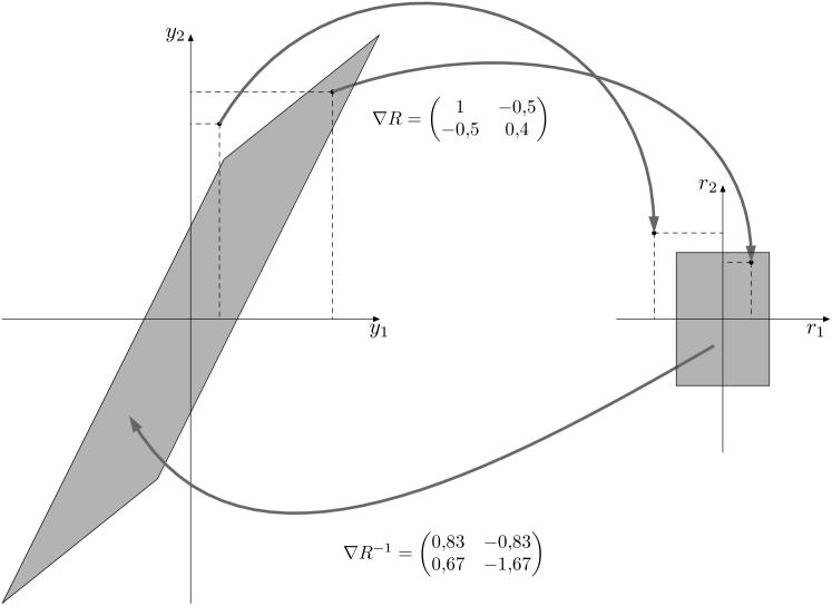
Figure 1: Insensitivity regions in different representation domains, y (left) and r (right), related by a non-diagonal transform $\nabla R$ and its inverse $\nabla R^{-1}$.

Summarizing, in the image coding context, the condition for an image representation y to be strictly suitable for conventional SVM learning is that the transform that maps the original representation y to an independent coefficient representation r must be locally diagonal.

As will be reviewed below, independence among coefficients (and the transforms to obtain them) may be defined in both statistical and perceptual terms (Hyvarinen et al., 2001; Malo et al., 2001; Epifanio et al., 2003; Malo et al., 2006). On the one hand, a locally diagonal relation to a statistically independent representation is desirable because independently induced distortions (as the conventional SVM approach does) will preserve the statistics of the distorted signal, that is, it will not introduce artificial-looking artifacts. On the other hand, a locally diagonal relation to a perceptually independent representation is desirable because independently induced distortions do not give rise to increased subjective distortions due to non-trivial masking or facilitation interactions between the distortions in each dimension (Watson and Solomon, 1997).

In this work, we show that conventional linear domains do not fulfill the diagonal Jacobian condition in either the statistical case or in the perceptual case. This theoretical result is experimentally confirmed by comparing SVM learning in previously reported linear domains (Robinson and Kecman, 2003; Gómez-Pérez et al., 2005) and in a recently proposed non-linear perceptual domain that simultaneously reduces the statistical and the perceptual relations (Malo et al., 2006), thus, this non-linear perceptual domain is closer to fulfilling the proposed condition.

The rest of the paper is structured as follows. Section 2 reviews the fact that linear coefficients of the image representations commonly used for SVM training are neither statistically independent nor perceptually independent. Section 3 shows that transforms for obtaining statistical and/or perceptual independence from linear domains have non-diagonal Jacobian. This suggests that there is room to improve the performance of conventional SVM learning reported in linear domains. In Section 4, we propose the use of a perceptual representation for SVM training because it strictly fulfills the diagonal Jacobian condition in the perceptual sense and increases the statistical independence among coefficients, bringing it closer to fulfilling the condition in the statistical sense. The experimental image coding results confirm the superiority of this domain for SVM training in Section 5. Section 6 presents the conclusions and final remarks.

2 Statistical and Perceptual Relations Among Image Coefficients

Statistical independence among the coefficients of a signal representation refers to the fact that the joint PDF of the class of signals to be considered can be expressed as a product of the marginal PDFs in each dimension (Hyvarinen et al., 2001). Simple (second-order) descriptions of statistical dependence use the non-diagonal nature of the covariance matrix (Clarke, 1985; Gersho and Gray, 1992). More recent and accurate descriptions use higher-order moments, mutual information, or the non-Gaussian nature (sparsity) of marginal PDFs (Hyvarinen et al., 2001; Simoncelli, 1997).

Perceptual independence refers to the fact that the visibility of errors in coefficients of an image may depend on the energy of neighboring coefficients, a phenomenon known in the perceptual literature as masking or facilitation (Watson and Solomon, 1997). Perceptual dependence has been formalized just up to second order, and this may be described by the non-Euclidean nature of the perceptual metric matrix (Malo et al., 2001; Epifanio et al., 2003; Malo et al., 2006).

2.1 Statistical Relations

In recent years, a variety of approaches, known collectively as “independent component analysis” (ICA), have been developed to exploit higher-order statistics for the purpose of achieving a unique linear solution for coefficient independence (Hyvarinen et al., 2001). The basis functions obtained when these methods are applied to images are spatially localized and selective for both orientation and spatial frequency (Olshausen and Field, 1996; Bell and Sejnowski, 1997). Thus, they are similar to basis functions of multi-scale wavelet representations.

Despite its name, linear ICA does not actually produce statistically independent coefficients when applied to photographic images. Intuitively, independence would seem unlikely, since images are not formed from linear superpositions of independent patterns: the typical combination rule for the elements of an image is occlusion. Empirically, the coefficients of natural image decompositions in spatially localized oscillating basis functions are found to be fairly well decorrelated (i.e., their covariance is almost zero). However, the amplitudes of coefficients at nearby spatial positions, orientations, and scales are highly correlated (even with orthonormal transforms) (Simoncelli, 1997; Buccigrossi and Simoncelli, 1999; Wainwright et al., 2001; Hyvarinen et al., 2003; Gutiérrez et al., 2006; Malo et al., 2006; Malo and Gutiérrez, 2006). This suggests that achieving statistical independence requires the introduction of non-linearities beyond linear ICA transforms.

Figure 2 reproduces one of many results that highlight the presence of statistical relations of natural image coefficients in block PCA or linear ICA-like domains: the energy of spatially localized oscillating filters is correlated with the energy of neighboring filters in scale and orientation (see Gutiérrez et al., 2006). A remarkable feature is that the interaction width increases with frequency, as has been reported in other domains, for example, wavelets (Buccigrossi and Simoncelli, 1999; Wainwright et al., 2001; Hyvarinen et al., 2003), and block-DCT (Malo et al., 2006).

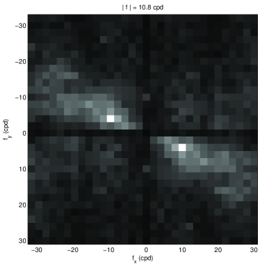
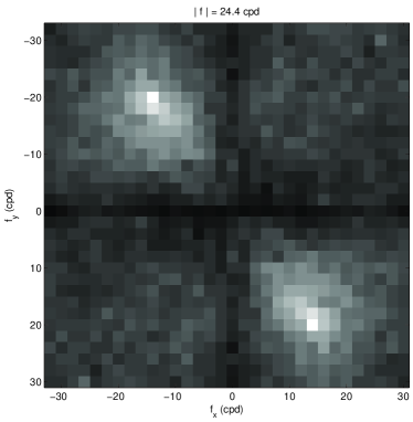
Figure 2: Statistical interaction of two particular coefficients of the local Fourier Transform with their neighbors in a natural image database. The absolute value of the frequency of these coefficients is $|f|=10.8$ and $|f|=24.4$ cycles/degree (cpd).

In order to remove the remaining statistical relations in the linear domains y, non-linear ICA methods are necessary (Hyvarinen et al., 2001; Lin, 1999; Karhunen et al., 2000; Jutten and Karhunen, 2003). Without lack of generality, non-linear ICA transforms can be schematically understood as a two-stage process (Malo and Gutiérrez, 2006):

$$\lx@xy@svg{\hbox{\raise 0.0pt\hbox{\kern 5.6389pt\hbox{\ignorespaces\ignorespaces\ignorespaces\hbox{\vtop{\kern 0.0pt\offinterlineskip\halign{\entry@#!@&&\entry@@#!@\cr&&\crcr}}}\ignorespaces{\hbox{\kern-5.6389pt\raise 0.0pt\hbox{\hbox{\kern 0.0pt\raise 0.0pt\hbox{\hbox{\kern 3.0pt\raise 0.0pt\hbox{$\textstyle{\mathbf{x}\ignorespaces\ignorespaces\ignorespaces\ignorespaces\ignorespaces\ignorespaces\ignorespaces\ignorespaces\ignorespaces\ignorespaces}$}}}}}}}\ignorespaces\ignorespaces\ignorespaces\ignorespaces\ignorespaces{}{}{}{{}{}{}{}{}{}{}{}{}{}{}{}{}{}{}{}{}{}}{}\ignorespaces\hbox{\hbox{\kern 0.0pt\raise 0.0pt\hbox{{}{}{{}}{{}{}{}}{}}}}\ignorespaces{}\ignorespaces{}{}{}{{}{}}\ignorespaces\ignorespaces{\hbox{\kern 12.11115pt\raise 11.39166pt\hbox{{}\hbox{\kern 0.0pt\raise 0.0pt\hbox{\hbox{\kern 3.0pt\hbox{\hbox{\kern 0.0pt\raise-2.39166pt\hbox{$\scriptstyle{\mathbf{T}}$}}}\kern 3.0pt}}}}}}\ignorespaces{}{}{}{{}{}{}{}{}{}{}{}{}{}{}{}{}{}{}{}{}{}{}{}{}}{\hbox{\kern 29.64084pt\raise 3.2222pt\hbox{\hbox{\kern 0.0pt\raise 0.0pt\hbox{\lx@xy@tip{1}\lx@xy@tip{-1}}}}}}\ignorespaces\hbox{\hbox{\kern 0.0pt\raise 0.0pt\hbox{{}{}{}{{}}{{}{}{}\lx@xy@spline@}{}}}}\ignorespaces{}\ignorespaces\hbox{\hbox{\kern 0.0pt\raise 0.0pt\hbox{{}{}{{}}{{}{}{}}{}}}}\ignorespaces{}\ignorespaces\ignorespaces\ignorespaces\ignorespaces\ignorespaces{}{}{}{{}{}{}{}{}{}{}{}{}{}{}{}{}}{\hbox{\kern 5.1677pt\raise-3.00064pt\hbox{\hbox{\kern 0.0pt\raise 0.0pt\hbox{\lx@xy@tip{1}\lx@xy@tip{-1}}}}}}\ignorespaces\hbox{\hbox{\kern 0.0pt\raise 0.0pt\hbox{{}{}{{}}{{}{}{}}{}}}}\ignorespaces{}\ignorespaces{}{}{}{{}{}}\ignorespaces\ignorespaces{\hbox{\kern 10.44447pt\raise-12.0361pt\hbox{{}\hbox{\kern 0.0pt\raise 0.0pt\hbox{\hbox{\kern 3.0pt\hbox{\hbox{\kern 0.0pt\raise-3.0361pt\hbox{$\scriptstyle{\mathbf{T^{-1}}}$}}}\kern 3.0pt}}}}}}\ignorespaces{}{}{}{{}{}{}{}{}{}{}{}{}{}{}{}{}{}{}{}{}{}{}{}{}}{}\ignorespaces\hbox{\hbox{\kern 0.0pt\raise 0.0pt\hbox{{}{}{}{{}}{{}{}{}\lx@xy@spline@}{}}}}\ignorespaces{}\ignorespaces\hbox{\hbox{\kern 0.0pt\raise 0.0pt\hbox{{}{}{{}}{{}{}{}}{}}}}\ignorespaces{}{\hbox{\kern 29.6389pt\raise 0.0pt\hbox{\hbox{\kern 0.0pt\raise 0.0pt\hbox{\hbox{\kern 3.0pt\raise 0.0pt\hbox{$\textstyle{\mathbf{y}\ignorespaces\ignorespaces\ignorespaces\ignorespaces\ignorespaces\ignorespaces\ignorespaces\ignorespaces\ignorespaces\ignorespaces}$}}}}}}}\ignorespaces\ignorespaces\ignorespaces\ignorespaces\ignorespaces{}{}{}{{}{}{}{}{}{}{}{}{}{}{}{}{}{}{}}{}\ignorespaces\hbox{\hbox{\kern 0.0pt\raise 0.0pt\hbox{{}{}{{}}{{}{}{}}{}}}}\ignorespaces{}\ignorespaces{}{}{}{{}{}}\ignorespaces\ignorespaces{\hbox{\kern 46.89188pt\raise 11.39166pt\hbox{{}\hbox{\kern 0.0pt\raise 0.0pt\hbox{\hbox{\kern 3.0pt\hbox{\hbox{\kern 0.0pt\raise-2.39166pt\hbox{$\scriptstyle{R}$}}}\kern 3.0pt}}}}}}\ignorespaces{}{}{}{{}{}{}{}{}{}{}{}{}{}{}{}{}{}{}{}{}{}{}{}}{\hbox{\kern 64.91693pt\raise 2.94655pt\hbox{\hbox{\kern 0.0pt\raise 0.0pt\hbox{\lx@xy@tip{1}\lx@xy@tip{-1}}}}}}\ignorespaces\hbox{\hbox{\kern 0.0pt\raise 0.0pt\hbox{{}{}{}{{}}{{}{}{}\lx@xy@spline@}{}}}}\ignorespaces{}\ignorespaces\hbox{\hbox{\kern 0.0pt\raise 0.0pt\hbox{{}{}{{}}{{}{}{}}{}}}}\ignorespaces{}\ignorespaces\ignorespaces\ignorespaces\ignorespaces\ignorespaces{}{}{}{{}{}{}{}{}{}{}{}{}{}{}{}{}{}{}}{\hbox{\kern 40.92017pt\raise-3.27574pt\hbox{\hbox{\kern 0.0pt\raise 0.0pt\hbox{\lx@xy@tip{1}\lx@xy@tip{-1}}}}}}\ignorespaces\hbox{\hbox{\kern 0.0pt\raise 0.0pt\hbox{{}{}{{}}{{}{}{}}{}}}}\ignorespaces{}\ignorespaces{}{}{}{{}{}}\ignorespaces\ignorespaces{\hbox{\kern 45.2252pt\raise-12.0361pt\hbox{{}\hbox{\kern 0.0pt\raise 0.0pt\hbox{\hbox{\kern 3.0pt\hbox{\hbox{\kern 0.0pt\raise-3.0361pt\hbox{$\scriptstyle{R^{-1}}$}}}\kern 3.0pt}}}}}}\ignorespaces{}{}{}{{}{}{}{}{}{}{}{}{}{}{}{}{}{}{}{}{}{}{}{}}{}\ignorespaces\hbox{\hbox{\kern 0.0pt\raise 0.0pt\hbox{{}{}{}{{}}{{}{}{}\lx@xy@spline@}{}}}}\ignorespaces{}\ignorespaces\hbox{\hbox{\kern 0.0pt\raise 0.0pt\hbox{{}{}{{}}{{}{}{}}{}}}}\ignorespaces{}{\hbox{\kern 64.9167pt\raise 0.0pt\hbox{\hbox{\kern 0.0pt\raise 0.0pt\hbox{\hbox{\kern 3.0pt\raise 0.0pt\hbox{$\textstyle{\mathbf{r}}$}}}}}}}\ignorespaces}}}}\ignorespaces, \textstyle{\mathbf{x}\ignorespaces\ignorespaces\ignorespaces\ignorespaces\ignorespaces\ignorespaces\ignorespaces\ignorespaces\ignorespaces\ignorespaces} \scriptstyle{\mathbf{T}} \scriptstyle{\mathbf{T^{-1}}} \textstyle{\mathbf{y}\ignorespaces\ignorespaces\ignorespaces\ignorespaces\ignorespaces\ignorespaces\ignorespaces\ignorespaces\ignorespaces\ignorespaces} \scriptstyle{R} \scriptstyle{R^{-1}} \textstyle{\mathbf{r}} \textstyle{\mathbf{x}\ignorespaces\ignorespaces\ignorespaces\ignorespaces\ignorespaces\ignorespaces\ignorespaces\ignorespaces\ignorespaces\ignorespaces} \scriptstyle{\mathbf{T}} \scriptstyle{\mathbf{T^{-1}}} \textstyle{\mathbf{y}\ignorespaces\ignorespaces\ignorespaces\ignorespaces\ignorespaces\ignorespaces\ignorespaces\ignorespaces\ignorespaces\ignorespaces} \scriptstyle{R} \scriptstyle{R^{-1}} \textstyle{\mathbf{r}}$$ (1)

where x is the image representation in the spatial domain, and $\mathbf{T}$ is a global unitary linear transform that removes second-order and eventually higher-order relations among coefficients in the spatial domain. Particular examples of $\mathbf{T}$ include block PCA, linear ICAs, DCT or wavelets. In the ICA literature notation, $\mathbf{T}$ is the separating matrix and $\mathbf{T^{-1}}$ is the mixing matrix. The second transform $R$ is an additional non-linearity that is introduced in order to remove the statistical relations that still remain in the y domain.

2.2 Perceptual Relations

Perceptual dependence among coefficients in different image representations can be understood by using the current model of V1 cortex. This model can also be summarized by the two-stage (linear and non-linear) process described in Equation (1). In this perceptual case, $\mathbf{T}$ is also a linear filter bank applied to the original input image in the spatial domain. This filter bank represents the linear behavior of V1 neurons whose receptive fields happen to be similar to wavelets or linear ICA basis functions (Olshausen and Field, 1996; Bell and Sejnowski, 1997). The second transform, $R$, is a non-linear function that accounts for the masking and facilitation phenomena that have been reported in the linear y domain (Foley, 1994; Watson and Solomon, 1997). Section 3.2 gives a parametric expression for the second non-linear stage, $R$: the divisive normalization model (Heeger, 1992; Foley, 1994; Watson and Solomon, 1997).

This class of models is based on psychophysical experiments assuming that the last domain, r, is perceptually Euclidean (i.e., perfect perceptual independence). An additional confirmation of this assumption is the success of (Euclidean) subjective image distortion measures defined in that domain (Teo and Heeger, 1994). Straightforward application of Riemannian geometry to obtain the perceptual metric matrix in other domains shows that the coefficients of linear domains x and y, or any other linear transform of them, are not perceptually independent (Epifanio et al., 2003).

Figure 3 illustrates the presence of perceptual relations between coefficients when using linear block frequency or wavelet-like domains, y: the cross-masking behavior. In this example, the visibility of the distortions added on top of the background image made of periodic patterns has to be assessed. This is a measure of the sensitivity of a particular perceptual mechanism to distortions in that dimension, $\Delta y_{f}$, when mechanisms tuned to other dimensions are simultaneously active, that is, $y_{f^{\prime}}\neq 0$, with $f^{\prime}\neq f$. As can be observed, low frequency noise is more visible in high frequency backgrounds than in low frequency backgrounds (e.g., left image). Similarly, high frequency noise is more visible in low frequency backgrounds than in high frequency ones (e.g., right image). That is to say, a signal of a specific frequency strongly masks the corresponding frequency analyzer, but it induces a smaller sensitivity reduction in the analyzers that are tuned to different frequencies. In other words, the reduction in sensitivity of a specific analyzer gets larger as the distance between the background frequency and the frequency of the analyzer gets smaller. The response of each frequency analyzer not only depends on the energy of the signal for that frequency band, but also on the energy of the signal in other frequency bands (cross-masking). This implies that a different amount of noise in each frequency band may be acceptable depending on the energy of that frequency band and on the energy of neighboring bands. This is what we have called perceptual dependence among different coefficients in the y domain.

3 cpd	6 cpd	12 cpd	24 cpd

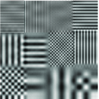
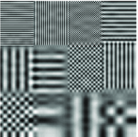
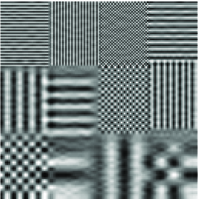
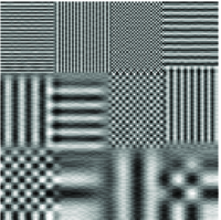
Figure 3: Illustrative example of perceptual dependence (cross-masking phenomenon). Equal energy noise of different frequency content, 3 cycl/deg (cpd), 6 cpd, 12 cpd and 24 cpd, shown on top of a background image. Sampling frequency assumes that these images subtend an angle of 3 deg.

At this point, it is important to stress the similarity between the set of computations to obtain statistically decoupled image coefficients and the known stages of biological vision. In fact, it has been hypothesized that biological visual systems have organized their sensors to exploit the particular statistics of the signals they have to process. See Barlow (2001), Simoncelli and Olshausen (2001), and Simoncelli (2003) for reviews on this hypothesis.

In particular, both the linear and the non-linear stages of the cortical processing have been successfully derived using redundancy reduction arguments: nowadays, the same class of linear stage T is used in transform coding algorithms and in vision models (Olshausen and Field, 1996; Bell and Sejnowski, 1997; Taubman and Marcellin, 2001), and new evidence supports the same idea for the second non-linear stage (Schwartz and Simoncelli, 2001; Malo and Gutiérrez, 2006). According to this, the statistical and perceptual transforms, $R$, that remove the above relations from the linear domains, y, would be very similar if not the same.

3 Statistical and Perceptual Independence Imply Non-diagonal Jacobian

In this section, we show that both statistical redundancy reduction transforms (e.g., non-linear ICA) and perceptual independence transforms (e.g., divisive normalization), have non-diagonal Jacobian for any linear image representation, so they are not strictly suitable for conventional SVM training.

3.1 Non-diagonal Jacobian in Non-linear ICA Transforms

One possible approach for dealing with global non-linear ICA is to act differentially by breaking the problem into local linear pieces that can then be integrated to obtain the global independent coefficient domain (Malo and Gutiérrez, 2006). Each differential sub-problem around a particular point (image) can be locally solved using the standard linear ICA methods restricted to the neighbors of that point (Lin, 1999).

Using the differential approach in the context of a two-stage process such as the one in Equation (1), it can be shown that (Malo and Gutiérrez, 2006):

$$\mathbf{r}=\mathbf{r_{0}}+\int_{\mathbf{x}_{0}}^{\mathbf{x}}\mathbf{T}_{\boldsymbol{\ell}}(\mathbf{x^{\prime}})\,d\mathbf{x^{\prime}}=\mathbf{r_{0}}+\int_{\mathbf{x}_{0}}^{\mathbf{x}}\nabla R(\mathbf{Tx^{\prime}})\,\mathbf{T}\,d\mathbf{x^{\prime}},$$ (2)

where $\mathbf{T}_{\boldsymbol{\ell}}(\mathbf{x^{\prime}})$ is the local separating matrix for a neighborhood of the image $\mathbf{x^{\prime}}$, and T is the global separating matrix for the whole PDF. Therefore, the Jacobian of the second non-linear stage is:

$$\nabla R(\mathbf{y})=\nabla R(\mathbf{T}\mathbf{x})=\mathbf{T}_{\boldsymbol{\ell}}(\mathbf{x})\,\mathbf{T^{-1}}.$$ (3)

As local linear independent features around a particular image, x, differ in general from global linear independent features, that is, $\mathbf{T}_{\boldsymbol{\ell}}(\mathbf{x})\neq\mathbf{T}$, the above product is not the identity nor diagonal in general.

3.2 Non-diagonal Jacobian in Non-linear Perceptual Transforms

The current response model for the cortical frequency analyzers is non-linear (Heeger, 1992; Watson and Solomon, 1997). The outputs of the filters of the first linear stage, y, undergo a non-linear sigmoid transform in which the energy of each linear coefficient is weighted by a linear Contrast Sensitivity Function (CSF) (Campbell and Robson, 1968; Malo et al., 1997) and is further normalized by a combination of the energies of neighbor coefficients in frequency,

$$r_{f}=R(\mathbf{y})_{f}=\frac{{\rm sgn}(y_{f})\,|\alpha_{f}\,y_{f}|^{\gamma}}{\beta_{f}+\sum_{f^{\prime}=1}^{n}h_{ff^{\prime}}|\alpha_{f^{\prime}}\,y_{f^{\prime}}|^{\gamma}},$$ (4)

where $\alpha_{f}$ (Figure 4[top left]) are CSF-like weights, $\beta_{f}$ (Figure 4[top right]) control the sharpness of the response saturation for each coefficient, $\gamma$ is the so called excitation exponent, and the matrix $h_{ff^{\prime}}$ determines the interaction neighborhood in the non-linear normalization of the energy. This interaction matrix models the cross-masking behavior (cf. Section 2.2). The interaction in this matrix is assumed to be Gaussian (Watson and Solomon, 1997), and its width increases with the frequency. Figure 4[bottom] shows two examples of this Gaussian interaction for two particular coefficients in a local Fourier domain. Note that the width of the perceptual interaction neighborhood increases with the frequency in the same way as the width of the statistical interaction neighborhood shown in Figure 2. We used a value of $\gamma=2$ in the experiments.

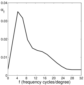
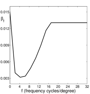
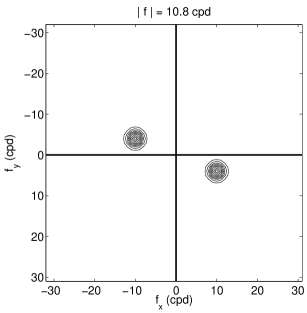
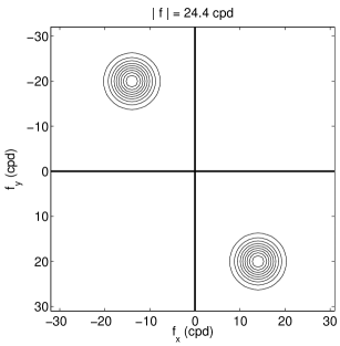
Figure 4: Parameters of the perceptual model: $\alpha_{f}$ (top left), $\beta_{f}$ (top right). Bottom figures represent perceptual interaction neighborhoods $h_{ff^{\prime}}$ of two particular coefficients of the local Fourier domain.

Taking derivatives in the general divisive normalization model, Equation (4), we obtain

$$\nabla R(\mathbf{y})_{ff^{\prime}}={\rm sgn}({y}_{f})\gamma\left(\frac{\alpha_{f}\,|\alpha_{f}\,y_{f}|^{\gamma-1}}{\beta_{f}+\sum_{f^{\prime}=1}^{n}h_{ff^{\prime}}|\alpha_{f^{\prime}}y_{{f^{\prime}}}|^{\gamma}}\delta_{ff^{\prime}}-\frac{\alpha_{f^{\prime}}|\alpha_{f}y_{f}|^{\gamma}|\alpha_{f^{\prime}}y_{f^{\prime}}|^{\gamma-1}}{(\beta_{f}+\sum_{f^{\prime}=1}^{n}h_{ff^{\prime}}|\alpha_{f^{\prime}}y_{{f^{\prime}}}|^{\gamma})^{2}}h_{ff^{\prime}}\right),$$ (5)

which is not diagonal because of the interaction matrix, $h$, which describes the cross-masking between each frequency $f$ and the remaining $f^{\prime}\neq f$.

Note that the intrinsic non-linear nature of both the statistical and perceptual transforms, Equations (3) and (5), makes the above results true for any linear domain under consideration. Specifically, if any other possible linear domain for image representation is considered, $\mathbf{y^{\prime}}=\mathbf{T^{\prime}}\,\mathbf{\mathbf{\mathbf{y}}}$, then the Jacobian of the corresponding independence transform, $R^{\prime}$, is

$$\nabla R^{\prime}(\mathbf{y^{\prime}})=\nabla R(\mathbf{y})\,\mathbf{T^{\prime-1}},$$

which, in general, will also be non-diagonal because of the non-diagonal and point-dependent nature of $\nabla R(\mathbf{y})$.

To summarize, since no linear domain fulfills the diagonal Jacobian condition in either statistical or perceptual terms, the negative situation illustrated in Figure 1 may occur when using SVM in these domains. Therefore, improved results could be obtained if SVM learning were applied after some transform achieving independent coefficients, $R$.

4 SVM Learning in a Perceptually Independent Representation

In order to confirm the above theoretical results (i.e., the unsuitability of linear representation domains for SVM learning) and to assess the eventual gain that can be obtained from training SVR in a more appropriate domain, we should compare the performance of SVRs in previously reported linear domains (e.g., block-DCT or wavelets) and in one of the proposed non-linear domains (either the statistically independent domain or the perceptually independent domain).

Exploration of the statistical independence transform may have academic interest but, in its present formulation, it is not practical for coding purposes: direct application of non-linear ICA as in Equation (2) is very time-consuming for high dimensional vectors since lots of local ICA computations are needed to transform each block, and a very large image database is needed for a robust and significant computation of $R$. Besides, an equally expensive differential approach is also needed to compute the inverse $R^{-1}$ for image decoding. In contrast, the perceptual non-linearity (and its inverse) are analytical. These analytical expressions are feasible for reasonable block sizes, and there are efficient iterative methods that can be used for larger vectors (Malo et al., 2006). In this paper, we explore the use of a psychophysically-based divisive normalized domain: first compute a block-DCT transform and then apply the divisive normalization model described above for each block. The results will be compared to the first competitive SVM coding results (Robinson and Kecman, 2003) and the posterior improvements reported by Gómez-Pérez et al. (2005), both formulated in the linear block-DCT domain.

As stated in Section 2, by construction, the proposed domain is perceptually Euclidean with perceptually independent components. The Euclidean nature of this domain has an additional benefit: the $\varepsilon$-insensitivity design is very simple because a constant value is appropriate due to the constant perceptual relevance of all coefficients. Thus, direct application of the standard SVR method is theoretically appropriate in this domain.

Moreover, beyond its built-in perceptual benefits, this psychophysically-based divisive normalization has attractive statistical properties: it strongly reduces the mutual information between the final coefficients r (Malo et al., 2006). This is not surprising according to the hypothesis that try to explain the early stages of biological vision systems using information theory arguments (Barlow, 1961; Simoncelli and Olshausen, 2001). Specifically, dividing the energy of each linear coefficient by the energy of the neighbors, which are statistically related with it, cf. Figure 2, gives coefficients with reduced statistical dependence. Moreover, as the empirical non-linearities of perception have been reproduced using non-linear ICA in Equation (2) (Malo and Gutiérrez, 2006), the empirical divisive normalization can be seen as a convenient parametric way to obtain statistical independence.

5 Performance of SVM Learning in Different Domains

In this section, we analyze the performance of SVM-based coding algorithms in linear and non-linear domains through rate-distortion curves and explicit examples for visual comparison. In addition, we discuss how SVM selects support vectors in these domains to represent the image features.

5.1 Model Development and Experimental Setup

In the (linear) block-DCT domain, ${\bf y}$, we use the method introduced by Robinson and Kecman (2003) (RKi-1), in which the SVR is trained to learn a fixed (low-pass) number of DCT coefficients (those with frequency bigger than 20 cycl/deg are discarded); and the method proposed by Gómez-Pérez et al. (2005) (CSF-SVR), in which the relevance of all DCT coefficients is weighted according to the CSF criterion using an appropriately modulated $\varepsilon_{f}$. In the non-linear domain, ${\bf r}$, we use the SVR with constant insensitivity parameter $\varepsilon$ (NL-SVR). In all cases, the block-size is 16$\times$16, that is, $\mathbf{y},\,\mathbf{r}\in\mathbb{R}^{256}$. The behavior of JPEG standard is also included in the experiments for comparison purposes.

As stated in Section 1, we used the RBF kernel and arbitrarily large penalization parameter in every SVR case. In all experiments, we trained the SVR models without the bias term, and modelled the absolute value of the DCT, y, or response coefficients, r. All the remaining free parameters ($\varepsilon$-insensitivity and Gaussian width of the RBF kernel $\sigma$) were optimized for all the considered models and different compression ratios. In the NL-SVM case, the parameters of the divisive normalization used in the experiments are shown in Figure 4. After training, the signal is described by the uniformly quantized Lagrange multipliers of the support vectors needed to keep the regression error below the thresholds $\varepsilon_{f}$. The last step is entropy coding of the quantized weights. The compression ratio is controlled by a factor applied to the thresholds, $\varepsilon_{f}$.

5.2 Model Comparison

In order to assess the quality of the coded images, three different measures were used: the standard (Euclidean) RMSE, the Maximum Perceptual Error (MPE) (Malo et al., 2000; Gómez-Pérez et al., 2005; Malo et al., 2006) and the also perceptually meaningful Structural SIMilarity (SSIM) index (Wang et al., 2004). Eight standard 256$\times$256 monochrome 8 bits/pix images were used in the experiments. Average rate-distortion curves are plotted in Figure 5 in the range [0.05, 0.6] bits/pix (bpp). According to these entropy-per-sample data, original file size was 64 KBytes in every case, while the compressed image sizes were in the range [0.4, 4.8] KBytes. This implies that the compression ratios were in the range [160:1, 13:1].

In general, a clear gain over standard JPEG is obtained by all SVM-based methods. According to the standard Euclidean MSE point of view, the performance of RKi-1 and CSF-SVR algorithms is basically the same (note the overlapped curves in Figure 5(a)). However, it is widely known that the MSE results are not useful to represent the subjective quality of images, as extensively reported elsewhere (Girod, 1993; Teo and Heeger, 1994; Watson and Malo, 2002). When using more appropriate (perceptually meaningful) quality measures (Figures 5(b)-(c)), the CSF-SVR obtains a certain advantage over the RKi-1 algorithm for all compression rates, which was already reported by Gómez-Pérez et al. (2005). In all measures, and for the whole considered entropy range, the proposed NL-SVR clearly outperforms all previously reported methods, obtaining a noticeable gain at medium-to-high compression ratios (between 0.1 bpp (80:1) and 0.3 bpp (27:1)). Taking into account that the recommended bit rate for JPEG is about 0.5 bpp, from Figure 5 we can also conclude that the proposed technique achieves the similar quality levels at a lower bit rate in the range [0.15, 0.3] bpp.

Figure 6 shows representative visual results of the considered SVM strategies on standard images (Lena and Barbara) at the same bit rate (0.3 bpp, 27:1 compression ratio or 2.4 KBytes in 256$\times$256 images). The visual inspection confirms that the numerical gain in MPE and SSIM shown in Figure 5 is also perceptually significant. Some conclusions can be extracted from this figure. First, as previously reported by Gómez-Pérez et al. (2005), RKi-1 leads to poorer (blocky) results because of the crude approximation of the CSF (as an ideal low-pass filter) and the equal relevance applied to the low-frequency DCT-coefficients. Second, despite the good performance yielded by the CSF-SVR approach to avoid blocking effects, it is worth noting that high frequency details are smoothed (e.g., see Barbara’s scarf). These effects are highly alleviated by introducing SVR in the non-linear domain. See, for instance, Lena’s eyes, her hat’s feathers or the better reproduction of the high frequency pattern in Barbara’s clothes.

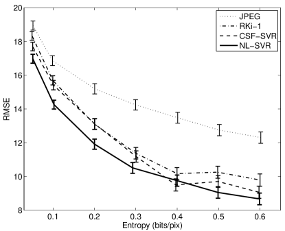
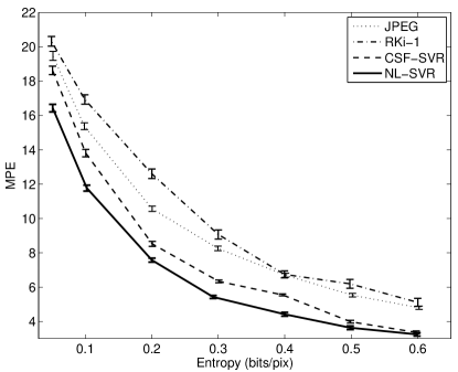
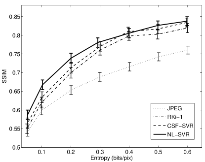
Figure 5: Average rate distortion curves over eight standard images (Lena, Barbara, Boats, Einstein, Peppers, Mandrill, Goldhill, Camera man) using objective and subjective measures for the considered JPEG (dotted) and the SVM approaches (RKi-1 dash-dotted, CSF-SVR dashed and NL-SVR solid). RMSE distortion (top), Maximum Perceptual Error, MPE (middle) (Malo et al., 2000; Gómez-Pérez et al., 2005; Malo et al., 2006), and Structural SIMilarity index, SSIM (bottom) (Wang et al., 2004).

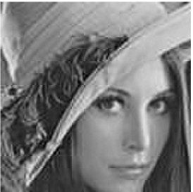
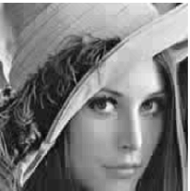
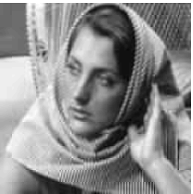
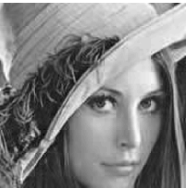
Figure 6: Examples of decoded Lena (left) and Barbara (right) images at 0.3 bits/pix. From top to bottom: JPEG, RKi-1, CSF-SVR, and NL-SVR.

Figure 7 shows the results obtained by all considered methods at a very high compression ratio for the Barbara image (0.05 bpp, 160:1 compression ratio or 0.4 KBytes in 256$\times$256 images). This experiment is just intended to show the limits of methods performance since it is out of the recommended rate ranges. Even though this scenario is unrealistic, differences among methods are still noticeable: the proposed NL-SVR method reduces the blocky effects (note for instance that the face is better reproduced). This is due to a better distribution of support vectors in the perceptually independent domain.

(a)	(b)
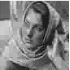
(c)	(d)

Figure 7: Examples of decoded Barbara images at a high compression ratio of 0.05 bits/pix (160:1) for (a) JPEG, (b) RKi-1, (c) CSF-SVR, and (d) NL-SVR.

5.3 Support Vector Distribution

The observed different perceptual image quality obtained with each approach is a direct consequence of support vector distribution in different domains. Figure 8 shows a representative example of the distribution of the selected support vectors by the RKi-1 and the CSF-SVR models working in the linear DCT domain, and the NL-SVM working in the perceptually independent non-linear domain r. Specifically, a block of Barbara’s scarf at different compression ratios is used for illustration purposes.

The RKi-1 approach (Robinson and Kecman, 2003) uses a constant $\varepsilon$ but, in order to consider the low subjective relevance of the high-frequency region, the corresponding coefficients are neglected. As a result, this approach only allocates support vectors in the low/medium frequency regions. The CSF-SVR approach uses a variable $\varepsilon$ according to the CSF and gives rise to a more natural concentration of support vectors in the low/medium frequency region, which captures medium to high frequency details at lower compression rates (0.5 bits/pix). Note that the number of support vectors is bigger than in the RKi-1 approach, but it selects some necessary high-frequency coefficients to keep the error below the selected threshold. However, for bigger compression ratios (0.3 bits/pix), it misrepresents some high frequency, yet relevant, features (e.g., the peak from the stripes). The NL-SVM approach works in the non-linear transform domain, in which a more uniform coverage of the domain is done, accounting for richer (and perceptually independent) coefficients to perform efficient sparse signal reconstruction.

(a)	(b)	(c)

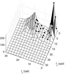
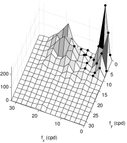
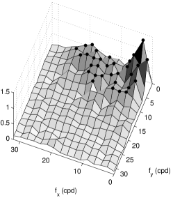
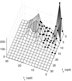
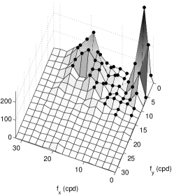
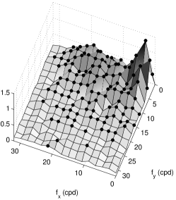
Figure 8: Signal in different domains and the selected support vectors by the SVM models in a block of the Barbara image at 0.3 bits/pix (top row) and 0.5 bits/pix (bottom row). Different domains are analyzed: (a) linear DCT using RKi-1, (b) linear DCT with CSF-SVM, and (c) non-linear perceptual domain with standard $\varepsilon$-SVM (NL-SVR).

It is important to remark that, for a given method (or domain), tightening $\varepsilon_{f}$ implies (1) considering more support vectors, and (2) an increase in entropy (top and bottom rows in Figure 8, 0.3 bpp to 0.5 bpp). However, note that the relevant measure is the entropy and not the number of support vectors: even though the number of selected support vectors in the $\mathbf{r}$ domain is higher, their variance is lower, thus giving rise to the same entropy after entropy coding.

6 Conclusions

In this paper, we have reported a condition on the suitable domain for developing efficient SVM image coding schemes. The so-called diagonal Jacobian condition states that SVM regression with scalar-wise error restriction in a particular domain makes sense only if the transform that maps this domain to an independent coefficient representation is locally diagonal. We have demonstrated that, in general, linear domains do not fulfill this condition because non-trivial statistical and perceptual inter-coefficient relations do exist in these domains.

This theoretical finding has been experimentally confirmed by observing that improved compression results are obtained when SVM is applied in a non-linear perceptual domain that starts from the same linear domain used by previously reported SVM-based image coding schemes. These results highlight the relevance of an appropriate image representation choice before SVM learning.

Further work is tied to the use of SVM-based coding schemes in statistically, rather than perceptually, independent non-linear ICA domains. In order to do so, local PCA instead of local ICA may be used in the local-to-global differential approach (Malo and Gutiérrez, 2006) to speed up the non-linear computation.

Acknowledgments

This work has been partly supported by the Spanish Ministry of Education and Science under grant CICYT TEC2006-13845/TCM and by the Generalitat Valenciana under grant GV-06/215.

References

- Ahmed (2005) R. Ahmed. Wavelet-based image compression using SVM learning and encoding techniques. Proc. 8th IASTED International Conference Computer Graphics and Imaging, 1:162–166, 2005.
- Barlow (1961) H. B. Barlow. Possible principles underlying the transformation of sensory messages. In WA Rosenblith, editor, Sensory Communication, pages 217–234. MIT Press, Cambridge, MA, 1961.
- Barlow (2001) H. B. Barlow. Redundancy reduction revisited. Network: Comp. Neur. Sys., 12:241–253, 2001.
- Bell and Sejnowski (1997) A. J. Bell and T. J. Sejnowski. The ‘independent components’ of natural scenes are edge filters. Vision Research, 37(23):3327–3338, 1997.
- Buccigrossi and Simoncelli (1999) R. W. Buccigrossi and E. P. Simoncelli. Image compression via joint statistical characterization in the wavelet domain. IEEE Transactions on Image Processing, 8(12):1688–1701, 1999.
- Campbell and Robson (1968) F. W. Campbell and J. G. Robson. Application of Fourier analysis to the visibility of gratings. Journal of Physiology, 197(3):551–566, August 1968.
- Camps-Valls et al. (2001) G. Camps-Valls, E. Soria-Olivas, J. Pérez-Ruixo, A. Artés-Rodríguez, F. Pérez-Cruz, and A. Figueiras-Vidal. A profile-dependent kernel-based regression for cyclosporine concentration prediction. In Neural Information Processing Systems (NIPS) – Workshop on New Directions in Kernel-Based Learning Methods, Vancouver, Canada, December 2001.
- Clarke (1985) R. J. Clarke. Transform Coding of Images. Academic Press, New York, 1985.
- Epifanio et al. (2003) I. Epifanio, J. Gutiérrez, and J. Malo. Linear transform for simultaneous diagonalization of covariance and perceptual metric matrix in image coding. Pattern Recognition, 36(8):1799–1811, August 2003.
- Foley (1994) J. M. Foley. Human luminance pattern mechanisms: Masking experiments require a new model. Journal of the Optical Society of America A, 11(6):1710–1719, 1994.
- Gersho and Gray (1992) A. Gersho and R. M. Gray. Vector Quantization and Signal Compression. Kluwer Academic Press, Boston, 1992.
- Girod (1993) B. Girod. What’s wrong with mean-squared error. In A. B. Watson, editor, Digital Images and Human Vision, pages 207–220. The MIT press, 1993.
- Gómez-Pérez et al. (2005) G. Gómez-Pérez, G. Camps-Valls, J. Gutiérrez, and J. Malo. Perceptually adaptive insensitivity for support vector machine image coding. IEEE Transactions on Neural Networks, 16(6):1574–1581, 2005.
- Gutiérrez et al. (2006) J. Gutiérrez, F. J. Ferri, and J. Malo. Regularization operators for natural images based on nonlinear perception models. IEEE Transactions on Image Processing, 15(1):189–2000, January 2006.
- Heeger (1992) D. J. Heeger. Normalization of cell responses in cat striate cortex. Vis. Neurosci., 9:181–198, 1992.
- Hyvarinen et al. (2001) A. Hyvarinen, J. Karhunen, and E. Oja. Independent Component Analysis. John Wiley & Sons, New York, 2001.
- Hyvarinen et al. (2003) A. Hyvarinen, J. Hurri, and J. Vayrynenm. Bubbles: a unifying framework for low-level statistical properties of natural image sequences. Journal of the Optical Society of America A, 20(7), 2003.
- Jiao et al. (2005) R. Jiao, Y. Li, Q. Wang, and B. Li. SVM regression and its application to image compression. In International Conference on Intelligent Computing, volume 3645, pages 747–756. Lecture Notes on Computer Science, 2005.
- Jutten and Karhunen (2003) C. Jutten and J. Karhunen. Advances in nonlinear blind source separation. Proc. of the 4th Int. Symp. on Independent Component Analysis and Blind Signal Separation (ICA2003), pages 245–256, 2003.
- Karhunen et al. (2000) J. Karhunen, S. Malaroiu, and M. Ilmoniemi. Local linear independent component analysis based on clustering. Intl. J. Neur. Syst., 10(6), December 2000.
- Lin (1999) J. K. Lin. Factorizing probability density functions: Generalizing ICA. In Proc. of the First Intl. Workshop on ICA and Signal Separation, pages 313–318, Aussois, France, 1999.
- Malo and Gutiérrez (2006) J. Malo and J. Gutiérrez. V1 non-linear properties emerge from local-to-global non-linear ICA. Network: Computation in Neural Systems, 17:85–102, 2006.
- Malo et al. (1997) J. Malo, A. M. Pons, A. Felipe, and J. M. Artigas. Characterization of human visual system threshold performance by a weighting function in the Gabor domain. Journal of Modern Optics, 44(1):127–148, 1997.
- Malo et al. (2000) J. Malo, F. Ferri, J. Albert, J. Soret, and J. M. Artigas. The role of perceptual contrast non-linearities in image transform coding. Image & Vision Computing, 18(3):233–246, February 2000.
- Malo et al. (2001) J. Malo, J. Gutiérrez, I. Epifanio, F. Ferri, and J. M. Artigas. Perceptual feed-back in multigrid motion estimation using an improved DCT quantization. IEEE Transactions on Image Processing, 10(10):1411–1427, October 2001.
- Malo et al. (2006) J. Malo, I. Epifanio, R. Navarro, and E. Simoncelli. Non-linear image representation for efficient perceptual coding. IEEE Transactions on Image Processing, 15(1):68–80, 2006.
- Olshausen and Field (1996) B. A. Olshausen and D. J. Field. Emergence of simple-cell receptive field properties by learning a sparse code for natural images. Nature, 381:607–609, 1996.
- Pérez-Cruz et al. (2002) F. Pérez-Cruz, G. Camps-Valls, E. Soria-Olivas, J. J. Pérez-Ruixo, A. R. Figueiras-Vidal, and A. Artés-Rodríguez. Multi-dimensional function approximation and regression estimation. In International Conference on Artificial Neural Networks, ICANN2002, Madrid, Spain., Aug 2002. Lecture Notes in Computer Science. Springer–Verlag.
- Robinson and Kecman (2000) J. Robinson and V. Kecman. The use of Support Vector Machines in image compression. In Proceedings of the International Conference on Engineering Intelligence Systems, EIS’2000, volume 36, pages 93–96, University of Paisley, Scotland, U.K., June 2000.
- Robinson and Kecman (2003) J. Robinson and V. Kecman. Combining Support Vector Machine learning with the discrete cosine transform in image compression. IEEE Transactions Neural Networks, 14(4):950–958, July 2003.
- Schwartz and Simoncelli (2001) O. Schwartz and E. P. Simoncelli. Natural signal statistics and sensory gain control. Nature Neuroscience, 4(8):819–825, 2001.
- Simoncelli (1997) E. P. Simoncelli. Statistical models for images: Compression, restoration and synthesis. In 31st Asilomar Conference on Signals, Systems and Computers, Pacific Grove, CA, 1997.
- Simoncelli (2003) E. P. Simoncelli. Vision and the statistics of the visual environment. Current Opinion in Neurobiology, 13(2):144–149, 2003.
- Simoncelli and Olshausen (2001) E. P. Simoncelli and B. O. Olshausen. Natural image statistics and neural representation. Annual Review of Neuroscience, 24:1193–1216, 2001.
- Smola and Schölkopf (2004) A. J. Smola and B. Schölkopf. A tutorial on support vector regression. Statistics and Computing, 14:199–222, 2004.
- Taubman and Marcellin (2001) D. S. Taubman and M. W. Marcellin. JPEG2000: Image Compression Fundamentals, Standards and Practice. Kluwer Academic Publishers, Boston, 2001.
- Teo and Heeger (1994) P. C. Teo and D. J. Heeger. Perceptual image distortion. Proceedings of the First IEEE International Conference on Image Processing, 2:982–986, 1994.
- Wainwright et al. (2001) M. J. Wainwright, E. P. Simoncelli, and A. S. Willsky. Random cascades on wavelet trees and their use in analyzing and modeling natural images. Applied and Computational Harmonic Analysis, 11:89–123, 2001.
- Wang et al. (2004) Z. Wang, A. C. Bovik, H. R. Sheikh, and E. P. Simoncelli. Image quality assessment: From error visibility to structural similarity. IEEE Transactions on Image Processing, 13(4):600–612, 2004.
- Watson and Malo (2002) A. B. Watson and J. Malo. Video quality measures based on the standard spatial observer. In Proceedings of the IEEE International Conference on Image Proceedings, volume 3, pages 41–44, 2002.
- Watson and Solomon (1997) A. B. Watson and J. A. Solomon. A model of visual contrast gain control and pattern masking. Journal of the Optical Society of America A, 14(9):2379–2391, September 1997.