Determining the Higgs spin and parity in the di-photon decay channel using gluon polarization

Abstract:

Gluons inside an unpolarized proton are in general linearly polarized. This polarization can, in principle, be used to determine the spin and parity of the newly found Higgs-like boson at the LHC. We focus here on the calculation of the degree of polarization.

With the discovery of a new Higgs-like particle at the LHC [1, 2] the task at hand is to verify, as accurately as possible, whether all its properties are those predicted by the Standard Model (SM). A specific property of the SM Higgs boson is its parity-even scalar coupling to other particles. This feature needs verification in all its production and decay channels independently.

In the gluon fusion production channel with a decay to two photons, the full process is characterized by only one single angle in the absence of gluon polarization. This polar angle $\theta$, between the diphoton axis and digluon axis in the partonic center of mass frame, does not contain any information on the parity of the coupling, nor can it be used to distinguish between all possible spin-2 coupling scenarios [3, 4, 5, 6, 7]. In the case that one or both of the incoming gluons are linearly polarized, the azimuthal distribution can also be non-trivial and, at the same time, will the gluon polarization modify the transverse momentum distribution of the produced Higgs-like particle.

A gluon extracted from an unpolarized proton is in general linearly polarized with a magnitude and direction depending on its transverse momentum. This effect is not taken into account in event generators, where the partonic transverse momentum is generated by parton showers that leave the gluons unpolarized. In earlier publications we reported on the effect of this gluon polarization on the transverse momentum distribution and azimuthal distribution of decay products in Higgs production [8, 9, 10] and how it can be used to determine its spin and parity. Here we will focus on the calculation of the degree of polarization.

Transverse Momentum Dependent factorization

To accurately describe Higgs boson production at small and moderate transverse momentum one needs to use the framework of Transverse Momentum Dependent (TMD) factorization. In that framework, the full $pp\to\gamma\gamma X$ cross section is split into a partonic $gg\to\gamma\gamma$ cross section and two TMD gluon correlators, which describe the distribution of gluons inside a proton as a function of not only its momentum along the direction of the proton, but also transverse to it. More specifically, the differential cross section for the inclusive production of a photon pair from gluon-gluon fusion is written as [11, 12, 13],

$$\frac{\mathrm{d}\sigma}{\mathrm{d}^{4}q\mathrm{d}\Omega}\propto\int\!\!\mathrm{d}^{2}{\bf p}_{\scriptscriptstyle T}\mathrm{d}^{2}{\bf k}_{\scriptscriptstyle T}\delta^{2}({\bf p}_{\scriptscriptstyle T}+{\bf k}_{\scriptscriptstyle T}-{\bf q}_{\scriptscriptstyle T})\mathcal{M}_{\mu\rho\kappa\lambda}\left(\mathcal{M}_{\nu\sigma}^{\quad\kappa\lambda}\right)^{*}\\ \Phi_{g}^{\mu\nu}(x_{1},{\bf p}_{\scriptscriptstyle T},\zeta_{1},\mu)\,\Phi_{g}^{\rho\sigma}(x_{2},{\bf k}_{\scriptscriptstyle T},\zeta_{2},\mu),$$ (1)

with the longitudinal momentum fractions $x_{1}={q\cdot P_{2}}/{P_{1}\cdot P_{2}}$ and $x_{2}={q\cdot P_{1}}/{P_{1}\cdot P_{2}}$, $q$ the momentum of the photon pair, $\mathcal{M}$ the $gg\to\gamma\gamma$ partonic hard scattering matrix element and $\Phi$ the following gluon TMD correlator in an unpolarized proton,

$$\Phi_{g}^{\mu\nu}(x,{\bf p}_{\scriptscriptstyle T},\zeta,\mu) \equiv\int\frac{\mathrm{d}(\xi\cdot P)\,\mathrm{d}^{2}\xi_{\scriptscriptstyle T}}{(xP\cdot n)^{2}(2\pi)^{3}}e^{i(xP+p_{\scriptscriptstyle T})\cdot\xi}\,\langle P|F_{a}^{n\nu}(0)\left(\mathcal{U}_{[0,\xi]}^{n[\text{--}]}\right)_{ab}F_{b}^{n\mu}(\xi)|P\rangle\Big{|}_{\xi\cdot P^{\prime}=0}$$

$$=-\frac{1}{2x}\bigg{\{}g_{\scriptscriptstyle T}^{\mu\nu}f_{1}^{g}(x,{\bf p}_{\scriptscriptstyle T}^{2},\zeta,\mu)-\bigg{(}\frac{p_{\scriptscriptstyle T}^{\mu}p_{\scriptscriptstyle T}^{\nu}}{M_{p}^{2}}\,{+}\,g_{\scriptscriptstyle T}^{\mu\nu}\frac{{\bf p}_{\scriptscriptstyle T}^{2}}{2M_{p}^{2}}\bigg{)}h_{1}^{\perp\,g}(x,{\bf p}_{\scriptscriptstyle T}^{2},\zeta,\mu)\bigg{\}}+\text{HT},$$ (2)

with $p_{{\scriptscriptstyle T}}^{2}=-{\bf p}_{\scriptscriptstyle T}^{2}$ and $g^{\mu\nu}_{{\scriptscriptstyle T}}=g^{\mu\nu}-P^{\mu}P^{\prime\nu}/P{\cdot}P^{\prime}-P^{\prime\mu}P^{\nu}/P{\cdot}P^{\prime}$, where $P$ and $P^{\prime}$ are the momenta of the colliding protons and $M_{p}$ their mass. The gauge link $\mathcal{U}_{[0,\xi]}^{n[\text{--}]}$ for this process arises from initial state interactions. It runs from $0$ to $\xi$ via minus infinity along the direction $n$, which is a time-like dimensionless four-vector with no transverse components such that $\zeta^{2}=(2n{\cdot}P)^{2}/n^{2}$. In principle, Eqs. (1) and (Transverse Momentum Dependent factorization) also contain soft factors, but with the appropriate choice of $\zeta$ (of around 1.5 times $\sqrt{s}$), one can neglect their contribution, at least up to next-to-leading order [11, 13]. To avoid the appearance of large logarithms in ${\cal M}$, the renormalization scale $\mu$ needs to be of order $M_{h}$. The second line of Eq. (Transverse Momentum Dependent factorization) contains the parameterization of the TMD correlator in terms of the unpolarized gluon distribution $f_{1}^{g}$, the linearly polarized gluon distribution $h_{1}^{\perp\,g}$ and Higher Twist (HT) terms, which only give $\mathcal{O}(1/Q)$ suppressed contributions to the cross section, where $Q\equiv\sqrt{q^{2}}$.

Degree of Polarization

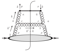
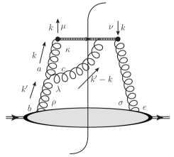
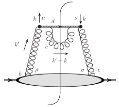
Figure 1: Feynman diagrams contributing to the tail of the gluon correlator.

The degree of polarization is defined as the linearly polarized gluon distribution with respect to its upper bound [14], i.e.,

$$\mathcal{P}(x,{\bf k}_{\scriptscriptstyle T}^{2},\zeta,\mu)\equiv\frac{h_{1}^{\perp g}(x,{\bf k}_{\scriptscriptstyle T}^{2},\zeta,\mu)}{\frac{2M_{p}^{2}}{{\bf k}_{\scriptscriptstyle T}^{2}}f_{1}^{g}(x,{\bf k}_{\scriptscriptstyle T}^{2},\zeta,\mu)},\text{ such that }|\mathcal{P}|\leq 1.$$ (3)

The tail of the gluon correlator (${\bf k}_{\scriptscriptstyle T}^{2}\gg M_{p}^{2}$) can be expressed in terms of the Feynman diagrams in Fig. 1 as

$$\Phi_{\text{tail}}^{\mu\nu}(x,{\bf k}_{\scriptscriptstyle T},\zeta,\mu)=\frac{\int\!\mathrm{d}(k\cdot P)}{(k\cdot n)^{2}}\left(\text{diag 1}+\text{diag 2}+\text{diag 3}\right).$$ (4)

The contributions from the three diagrams to the tail are

$$\Phi^{\mu\nu}_{\mathrm{diag1}}= \frac{4\pi\alpha_{s}}{(k{\cdot}n)^{2}}f^{abc}f^{aec}\!\!\int\frac{\mathrm{d}^{4}(k^{\prime}-k)\mathrm{d}(k{\cdot}P)}{(2\pi)^{3}}\delta\Big{[}(k^{\prime}-k)^{2}\Big{]}\frac{\Big{[}k\cdot ng^{\mu}_{\kappa}-k^{\mu}n_{\kappa}\Big{]}\Big{[}k\cdot ng^{\nu}_{\eta}-k^{\nu}n_{\eta}\Big{]}}{k^{4}}\Phi_{\rho\sigma}^{be}(k^{\prime})$$

$$\Big{[}g^{\kappa\lambda}(k^{\prime} -2k)^{\rho}+g^{\lambda\rho}(k-2k^{\prime})^{\kappa}+g^{\rho\kappa}(k^{\prime}+k)^{\lambda}\Big{]}\Big{[}g_{\lambda}^{\eta}(2k-k^{\prime})^{\sigma}+g_{\lambda}^{\sigma}(2k^{\prime}-k)^{\eta}+g^{\eta\sigma}(-k^{\prime}-k)_{\lambda}\Big{]}$$

$$\Phi^{\mu\nu}_{\mathrm{diag2}}= \frac{4\pi\alpha_{s}}{(k{\cdot}n)^{2}}f^{abc}f^{ace}\!\!\int\frac{\mathrm{d}^{4}(k^{\prime}-k)\mathrm{d}(k{\cdot}P)}{(2\pi)^{3}}\delta\Big{[}(k^{\prime}-k)^{2}\Big{]}\Big{[}k\cdot ng^{\mu}_{\kappa}-k^{\mu}n_{\kappa}\Big{]}\Big{[}k\cdot ng^{\nu\sigma}-k^{\prime\nu}n^{\sigma}\Big{]}\Phi_{\rho\sigma}^{be}(k^{\prime})$$

$$\frac{1}{k^{2}}\frac{n_{\lambda}}{(k^{\prime}-k)\cdot n}\Big{[}g^{\kappa\lambda}(k^{\prime}-2k)^{\rho}+g^{\lambda\rho}(k-2k^{\prime})^{\kappa}+g^{\rho\kappa}(k^{\prime}+k)^{\lambda}\Big{]}+\left(\mu\leftrightarrow\nu\right)$$

$$\Phi^{\mu\nu}_{\mathrm{diag3}}= \frac{4\pi\alpha_{s}}{(k{\cdot}n)^{2}}f^{bcd}f^{ced}\!\!\int\frac{\mathrm{d}^{4}(k^{\prime}-k)\mathrm{d}(k{\cdot}P)}{(2\pi)^{3}}\delta\Big{[}(k^{\prime}-k)^{2}\Big{]}\Big{[}k\cdot ng^{\mu\rho}-k^{\prime\mu}n^{\rho}\Big{]}\Big{[}k\cdot ng^{\nu\sigma}-k^{\prime^{\nu}}n^{\sigma}\Big{]}$$

$$\Phi_{\rho\sigma}^{be}(k^{\prime})\frac{n^{2}}{[(k^{\prime}-k)\cdot n]^{2}}$$ (5)

In the following calculation, the momenta $k$, $k^{\prime}$ and $n$ will be parameterized as

$$k =xP+k_{\scriptscriptstyle T}+\frac{k\cdot P}{P\cdot P^{\prime}}P^{\prime},$$

$$k^{\prime} =yP+k^{\prime}_{\scriptscriptstyle T}+\frac{k^{\prime}\cdot P}{P\cdot P^{\prime}}P^{\prime},$$

$$n =\frac{\sqrt{n^{2}}}{\zeta}P+\frac{\sqrt{n^{2}}\zeta}{2P\cdot P^{\prime}}P^{\prime},$$ (6)

in terms of the light-like vectors $P$ and $P^{\prime}$. Note that $k_{\scriptscriptstyle T}^{2}=-{\bf k}_{\scriptscriptstyle T}^{2}$. In the parameterization of the Lorentz structure we do not want $P$ and $P^{\prime}$, but rather $k_{\scriptscriptstyle T}$, $k$ and $n$, so the inverse relations are also useful,

$$P =-\frac{\zeta^{2}}{2k\cdot P-x\zeta^{2}}(k-k_{\scriptscriptstyle T})+\frac{2\zeta P\cdot P^{\prime}}{2k\cdot P-x\zeta^{2}}\frac{n}{\sqrt{n^{2}}},$$

$$P^{\prime} =\frac{2P\cdot P^{\prime}}{2k\cdot P-x\zeta^{2}}(k-k_{\scriptscriptstyle T})-\frac{2x\zeta P\cdot P^{\prime}}{2k\cdot P-x\zeta^{2}}\frac{n}{\sqrt{n^{2}}}.$$ (7)

The phase space becomes in this parameterization

$$\int\mathrm{d}^{4}(k^{\prime}-k)=\frac{1}{P\cdot P^{\prime}}\int\mathrm{d}(k^{\prime}\cdot P)\,\mathrm{d}(k^{\prime}\cdot P^{\prime})\,\mathrm{d}^{2}k_{\scriptscriptstyle T}^{\prime}=\int\mathrm{d}(k^{\prime}\cdot P)\,\mathrm{d}y\,\mathrm{d}^{2}k_{\scriptscriptstyle T}^{\prime}$$ (8)

The delta function that sets the emitted gluon on-shell will be removed by the integration over $k\cdot P$, i.e.,

$$\int\mathrm{d}(k\cdot P)\delta\Big{[}(k^{\prime}-k)^{2}\Big{]}=\int\mathrm{d}(k\cdot P)\delta\Big{(}2(y-x)(k^{\prime}-k)\cdot P+(k_{\scriptscriptstyle T}^{\prime}-k_{\scriptscriptstyle T})^{2}\Big{)}=\frac{1}{2(y-x)},$$ (9)

which sets

$$k\cdot P=\frac{(k_{\scriptscriptstyle T}^{\prime}-k_{\scriptscriptstyle T})^{2}}{2(y-x)}+k^{\prime}\cdot P.$$ (10)

The next step is to use the fact that $k^{\prime}\cdot P\ll k_{\scriptscriptstyle T}^{2}$ and $k_{\scriptscriptstyle T}^{\prime 2}\ll k_{\scriptscriptstyle T}^{2}$. We will make a zeroth order expansion in these small variables of the integrand, such that it does not depend on them anymore. This allows us to move everything out of the integral and express the tail of the TMD correlator in terms of the collinear correlator,

$$\int\!\mathrm{d}^{2}k_{\scriptscriptstyle T}^{\prime}\int\!\mathrm{d}(k^{\prime}\cdot P)\,\Phi^{\rho\sigma}(k^{\prime})=\Phi^{\rho\sigma}(y)=-\frac{1}{2y}g_{\scriptscriptstyle T}^{\rho\sigma}f_{1}^{g}(y,\mu_{0}),$$

where $f_{1}^{g}(y,\mu_{0})$ is the collinear gluon parton distribution function evaluated at a scale $\mu_{0}^{2}\ll k_{\scriptscriptstyle T}^{2}$. The resulting expressions can be cast in the following form

$$\Phi^{\mu\nu}_{\textrm{diag }i}(x,{\bf k}_{\scriptscriptstyle T},\zeta,\mu)=\frac{\alpha_{s}C_{A}}{4\pi^{2}}\int\!\mathrm{d}y\Big{[}A_{i}\,g_{\scriptscriptstyle T}^{\mu\nu}+B_{i}\,k_{\scriptscriptstyle T}^{\mu}k_{\scriptscriptstyle T}^{\nu}+C_{i}(n\cdot kn^{\mu}-n^{2}k^{\mu})(n\cdot kn^{\nu}-n^{2}k^{\nu})\\ +D_{i}\big{[}(n\cdot kn^{\mu}-n^{2}k^{\mu})k_{\scriptscriptstyle T}^{\nu}+k_{\scriptscriptstyle T}^{\nu}(n\cdot kn^{\mu}-n^{2}k^{\nu})\big{]}\Big{]}f_{1}^{g}(y,\mu_{0}),$$ (11)

in which the following coefficients are nonzero,

$$A_{1} =\frac{3y-2x}{k_{\scriptscriptstyle T}^{2}y^{3}}, B_{1} =\frac{4(y-x)^{3}(\zeta^{4}y^{2}-2\zeta^{2}k_{\scriptscriptstyle T}^{2})}{k_{\scriptscriptstyle T}^{4}y^{3}[k_{\scriptscriptstyle T}^{2}+\zeta^{2}x(x-y)]^{2}},$$

$$C_{1} =\frac{16\zeta^{4}(y-x)^{3}(2x^{2}-2xy+y^{2})}{n^{4}y^{3}[k_{\scriptscriptstyle T}^{4}-\zeta^{4}x^{2}(x-y)^{2}]^{2}}, D_{1} =-\frac{8\zeta^{2}(x-y)^{3}(\zeta^{2}(x^{2}-xy+y^{2})-k_{\scriptscriptstyle T}^{2})}{k_{\scriptscriptstyle T}^{2}n^{2}y^{3}[k_{\scriptscriptstyle T}^{2}-\zeta^{2}x(y-x)]^{2}[k_{\scriptscriptstyle T}^{2}+\zeta^{2}x(y-x)]},$$

$$A_{2} =\frac{k_{\scriptscriptstyle T}^{2}+\zeta^{2}(y^{2}-x^{2})}{k_{\scriptscriptstyle T}^{2}y^{2}[\zeta^{2}(x-y)^{2}-k_{\scriptscriptstyle T}^{2}]}, D_{2} =-\frac{4\zeta^{2}(x-y)^{2}}{k_{\scriptscriptstyle T}^{2}n^{2}y^{2}[\zeta^{2}(x-y)^{2}-k_{\scriptscriptstyle T}^{2}][k_{\scriptscriptstyle T}^{2}+\zeta^{2}x(y-x)]},$$

$$A_{3} =\frac{2\zeta^{2}(y-x)}{y[k_{\scriptscriptstyle T}^{2}-\zeta^{2}(x-y)^{2}]^{2}}.$$ (12)

Comparing Eq. (Transverse Momentum Dependent factorization) with Eq. (11) one can read off that the distribution functions are, in terms of these coefficients, given by

$$f_{1\textrm{tail}}^{g}(x,{\bf k}_{\scriptscriptstyle T}^{2},\zeta,\mu) =-\frac{x\alpha_{s}C_{A}}{2\pi^{2}}\int\!\mathrm{d}y\,\sum_{i}\left(A_{i}+\frac{k_{\scriptscriptstyle T}^{2}}{2}B_{i}\right)f_{1}^{g}(y,\mu_{0}),$$

$$h_{1\textrm{tail}}^{\perp g}(x,{\bf k}_{\scriptscriptstyle T}^{2},\zeta,\mu) =\frac{x\alpha_{s}C_{A}M_{p}^{2}}{2\pi^{2}}\int\!\mathrm{d}y\,\sum_{i}B_{i}f_{1}^{g}(y,\mu_{0}).$$ (13)

Note that at this order the tail of the distribution functions does not depend on the UV regulator $\mu$.

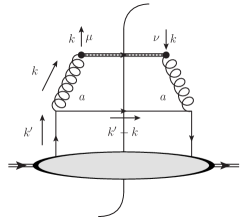
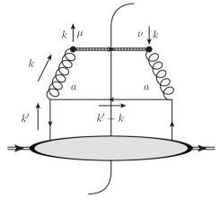
Figure 2: Quark initiated Feynman diagrams contributing to the tail of the gluon correlator.

Quark contribution

There will also be a contribution from the quark and anti-quark initiated diagrams depicted in Fig. 2. Those contributions can be calculated in the same way, yielding

$$\Phi^{\mu\nu}_{\mathrm{quark}}(x,{\bf k}_{\scriptscriptstyle T})=\frac{\alpha_{s}C_{F}}{4\pi^{2}}\int\!\mathrm{d}y\Big{[}A_{q}g_{\scriptscriptstyle T}^{\mu\nu}+B_{q}k_{\scriptscriptstyle T}^{\mu}k_{\scriptscriptstyle T}^{\nu}+C_{q}(n\cdot kn^{\mu}-n^{2}k^{\mu})(n\cdot kn^{\nu}-n^{2}k^{\nu})\\ +D_{q}\big{[}(n\cdot kn^{\mu}-n^{2}k^{\mu})k_{\scriptscriptstyle T}^{\nu}+k_{\scriptscriptstyle T}^{\nu}(n\cdot kn^{\mu}-n^{2}k^{\nu})\big{]}\Big{]}\sum_{q,\bar{q}}f_{1}^{q}(y,\mu_{0}),$$ (14)

with the coefficients

$$A_{q} =\frac{1}{k_{\scriptscriptstyle T}^{2}y^{2}}, B_{q} =-\frac{4\zeta^{2}(x-y)^{2}[k_{\scriptscriptstyle T}^{2}+\zeta^{2}y(x-y)]}{k_{\scriptscriptstyle T}^{4}y^{2}[k_{\scriptscriptstyle T}^{2}+\zeta^{2}x(x-y)]^{2}},$$

$$C_{q} =-\frac{16\zeta^{4}(x-y)^{5}}{n^{4}y^{2}[k_{\scriptscriptstyle T}^{4}-\zeta^{4}x^{2}(x-y)^{2}]^{2}}, D_{q} =\frac{4\zeta^{2}(x-y)^{3}[k_{\scriptscriptstyle T}^{2}-\zeta^{2}(x-2y)(x-y)]}{k_{\scriptscriptstyle T}^{2}n^{2}y^{2}[k_{\scriptscriptstyle T}^{2}+\zeta^{2}x(x-y)]^{2}[k_{\scriptscriptstyle T}^{2}+\zeta^{2}x(y-x)]}.$$ (15)

Their contribution to the distribution functions is given by

$$f_{1\text{tail}}^{g}(x,{\bf k}_{\scriptscriptstyle T}^{2},\zeta,\mu) =-\frac{x\alpha_{s}C_{F}}{2\pi^{2}}\int\!\mathrm{d}y\,\left(A_{q}+\frac{k_{\scriptscriptstyle T}^{2}}{2}B_{q}\right)\sum_{q,\bar{q}}\,f_{1}^{q}(y,\mu_{0}),$$

$$h_{1\text{tail}}^{\perp g}(x,{\bf k}_{\scriptscriptstyle T}^{2},\zeta,\mu) =\frac{x\alpha_{s}C_{F}M_{p}^{2}}{2\pi^{2}}\int\!\mathrm{d}y\,B_{q}\,\sum_{q,\bar{q}}\,f_{1}^{q}(y,\mu_{0}).$$ (16)

The $\zeta\to\infty$ limit

Calculations in the literature are often performed in the $\zeta\to\infty$ limit, in which we get

$$f_{1\text{tail}}^{g}(x,{\bf k}_{\scriptscriptstyle T}^{2},\zeta,\mu)= -\frac{\alpha_{s}}{\pi^{2}k_{\scriptscriptstyle T}^{2}}\int_{x}^{1}\!\frac{\mathrm{d}z}{z}\Bigg{[}C_{A}\bigg{\{}\frac{1-z}{z}+z(1-z)+\frac{z}{(1-z)^{+}}-\frac{1}{2}\delta(z-1)\times$$

$$\left(1+\log\left[\frac{-k_{\scriptscriptstyle T}^{2}}{x^{2}(1-x)^{2}\zeta^{2}}\right]\right)\bigg{\}}f_{1}^{g}\left(\frac{x}{z},\mu_{0}\right)+C_{F}\frac{1+(1-z)^{2}}{2z}\sum_{q,\bar{q}}f_{1}^{q}\left(\frac{x}{z},\mu_{0}\right)\Bigg{]},$$

$$h_{1\text{tail}}^{\perp g}(x,{\bf k}_{\scriptscriptstyle T}^{2},\zeta,\mu)= \frac{\alpha_{s}}{\pi^{2}k_{\scriptscriptstyle T}^{2}}\frac{2M_{p}^{2}}{k_{\scriptscriptstyle T}^{2}}\int_{x}^{1}\!\frac{\mathrm{d}z}{z}\frac{1-z}{z}\Bigg{[}C_{A}f_{1}^{g}\left(\frac{x}{z},\mu_{0}\right)+C_{F}\sum_{q,\bar{q}}f_{1}^{q}\left(\frac{x}{z},\mu_{0}\right)\Bigg{]}.$$ (17)

Results

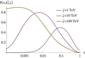
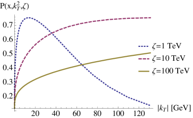
Figure 3: Degree of polarization plotted as a function of $x$ for fixed $|{\bf k}_{\scriptscriptstyle T}|=100$ GeV (left) and as function of $|{\bf k}_{\scriptscriptstyle T}|$ at fixed $x=125/8000$ (right) for various choices of $\zeta$.

Adding the gluon and (anti)quark initiated contributions, the degree of polarization can, for arbitrary $\zeta$ and large ${\bf k}_{\scriptscriptstyle T}$, be written as

$$\mathcal{P}(x,{\bf k}_{\scriptscriptstyle T}^{2},\zeta,\mu)=\frac{\frac{k_{\scriptscriptstyle T}^{2}}{2}\int_{x}^{1}\!\mathrm{d}y\left[C_{A}B_{1}f_{1}^{g}(y,\mu_{0})+C_{F}B_{q}\sum\limits_{q,\bar{q}}f_{1}^{q}(y,\mu_{0})\right]}{\int_{x}^{1}\!\mathrm{d}y\left[C_{A}\left(A_{1}+A_{2}+A_{3}+\frac{k_{\scriptscriptstyle T}^{2}}{2}B_{1}\right)f_{1}^{g}(y,\mu_{0})+C_{F}\left(A_{q}+\frac{k_{\scriptscriptstyle T}^{2}}{2}B_{q}\right)\sum\limits_{q,\bar{q}}f_{1}^{q}(y,\mu_{0})\right]},$$ (18)

up to corrections of $\mathcal{O}(\alpha_{s})$. The degree of polarization is plotted in Fig. 3 as a function of $x$ for fixed $|{\bf k}_{\scriptscriptstyle T}|=100$ GeV and as function of $|{\bf k}_{\scriptscriptstyle T}|$ at fixed $x=125/8000$ for various choices of $\zeta$, calculated from the MSTW 2008 parton distributions [15] evaluated at $\mu_{0}=2$ GeV. One can see that at the values of $x$ and $\zeta$ relevant for Higgs production at the LHC ($\sim 125/8000$ and $\sim 12$ TeV) the degree of polarization is substantial, reaching up to values larger than 70%.

Summary

Gluons inside an unpolarized proton are in general linearly polarized with a direction and magnitude depending on their transverse momentum. This polarization can, in principle, be used to determine the spin and parity of the newly found Higgs-like boson at the LHC as proposed in [10]. We have here elaborated on the perturbative calculation of the degree of polarization, which was used in [10]. Numerical results have been given for the degree of polarization as a function of the longitudinal momentum fraction $x$ and the transverse momentum $|{\bf k}_{\scriptscriptstyle T}|$, for various choices of the gauge link direction (or hadron energy) $\zeta^{2}\equiv(2n{\cdot}P)^{2}/n^{2}$. At the values of $x$ and $\zeta$ relevant for Higgs production at the LHC the degree of polarization is substantial, reaching up to values larger than 70%.

- [1] G. Aad et al. [ATLAS Collaboration], Phys. Lett. B 716, 1 (2012)
- [2] S. Chatrchyan et al. [CMS Collaboration], Phys. Lett. B 716, 30 (2012)
- [3] S. Y. Choi, D. J. Miller, M. M. Muhlleitner and P. M. Zerwas, Phys. Lett. B 553, 61 (2003)
- [4] Y. Gao, A. V. Gritsan, Z. Guo, K. Melnikov, M. Schulze and N. V. Tran, Phys. Rev. D 81, 075022 (2010)
- [5] S. Bolognesi, Y. Gao, A. V. Gritsan, K. Melnikov, M. Schulze, N. V. Tran and A. Whitbeck, Phys. Rev. D 86, 095031 (2012)
- [6] S. Y. Choi, M. M. Muhlleitner and P. M. Zerwas, Phys. Lett. B 718, 1031 (2013)
- [7] J. Ellis, R. Fok, D. S. Hwang, V. Sanz and T. You, Eur. Phys. J. C 73, 2488 (2013)
- [8] D. Boer, W. J. den Dunnen, C. Pisano, M. Schlegel and W. Vogelsang, Phys. Rev. Lett. 108, 032002 (2012)
- [9] W. J. den Dunnen, D. Boer, C. Pisano, M. Schlegel and W. Vogelsang, arXiv:1205.6931 [hep-ph].
- [10] D. Boer, W. J. den Dunnen, C. Pisano and M. Schlegel, Phys. Rev. Lett. 111, 032002 (2013)
- [11] X. -d. Ji, J. -P. Ma and F. Yuan, JHEP 0507, 020 (2005)
- [12] P. Sun, B. -W. Xiao and F. Yuan, Phys. Rev. D 84, 094005 (2011)
- [13] J. P. Ma, J. X. Wang and S. Zhao, Phys. Rev. D 88, 014027 (2013)
- [14] P. J. Mulders and J. Rodrigues, Phys. Rev. D 63, 094021 (2001)
- [15] A. D. Martin, W. J. Stirling, R. S. Thorne and G. Watt, Eur. Phys. J. C 63, 189 (2009)