Compressed Vertical Partitioning for Full-In-Memory RDF Management

Abstract

The Web of Data has been gaining momentum in recent years. This leads to increasingly publish more and more semi-structured datasets following, in many cases, the RDF data model based on atomic triple units of subject, predicate, and object. Although it is a very simple model, specific compression methods become necessary because datasets are increasingly larger and various scalability issues arise around their organization and storage. This requirement is even more restrictive in RDF stores because efficient SPARQL resolution on the compressed RDF datasets is also required.

This article introduces a novel RDF indexing technique that supports efficient SPARQL resolution in compressed space. Our technique, called k²-triples, uses the predicate to vertically partition the dataset into disjoint subsets of pairs (subject, object), one per predicate. These subsets are represented as binary matrices of subjects $\times$ objects in which 1-bits mean that the corresponding triple exists in the dataset. This model results in very sparse matrices, which are efficiently compressed using k²-trees. We enhance this model with two compact indexes listing the predicates related to each different subject and object in the dataset, in order to address the specific weaknesses of vertically partitioned representations. The resulting technique not only achieves by far the most compressed representations, but also achieves the best overall performance for RDF retrieval in our experimental setup. Our approach uses up to $10$ times less space than a state of the art baseline, and outperforms its time performance by several order of magnitude on the most basic query patterns. In addition, we optimize traditional join algorithms on k²-triples and define a novel one leveraging its specific features. Our experimental results show that our technique also overcomes traditional vertical partitioning for join resolution, reporting the best numbers for joins in which the non-joined nodes are provided, and being competitive in the great majority of the cases.

1 Introduction

The Resource Description Framework (RDF) (?) provides a simple scheme for structuring and linking data that describe facts of the world (?). It models knowledge in the form of triples (subject, predicate, object), in which the subject represents the resource being described, the predicate is the property, and the object contains the value associated to the property for the given subject. RDF was originally conceived (under a document-centric perspective of the Web) as a foundation for processing metadata and describing resources. However, this conception does not address its actual usage. The current Recommendation considers RDF as the key to do for machine processable information (application data) what the WWW has done for hypertext, that is, to allow data to be processed outside the particular environment in which it was created, in a fashion that can work at Internet scale. This statement describes the RDF status in the so-called Web of Data.

The Web of Data materializes the basic principles of the Semantic Web (?) and interconnects datasets from diverse fields of knowledge within a cloud of data-to-data hyperlinks that enables a ubiquitious and seamless data integration to the lowest level of granularity. Thus, information follows a data-centric organization within the Web of Data. The advancement in extraction mechanisms (?) or the annotation of massive amounts of resources (?), among others, have motivated the growth of the Web of Data in which the number (and scale) of semantic applications in use increases, more RDF data are linked together, and increasingly larger datasets are obtained. This popularity is the basis for the development of RDF management systems (referred to as RDF stores), which play a central role in the Web of Data. They provide support for RDF storage and also lookup infrastructure to access it via SPARQL (?) query interfaces. Although the increased amount of RDF available is good for semantic initiatives, it is also causing performance bottlenecks in the RDF stores currently used (?). Thus, scalability arises as a major issue, restricting popular RDF applications, like inference-based ones, because traditional solutions are not suitable for large-scale deployments (?). The scalability management is closely related to the RDF physical organization, storage and the mechanisms designed for its retrieval.

Two families of RDF stores are mainly used within the current Web of Data. On the one hand, relational stores are built on the generality, scalability, and maturity of relational databases. Some logical models have been proposed for organizing and storing RDF in relational stores (?). However, the relational model is quite strict to fit semi-structured RDF features, and these systems reach only limited success. On the other hand, native solutions are custom designed from scratch and focus directly on specific RDF features. Although various techniques have been proposed, multi-indexing ones are the most used within the current state of the art (?; ?; ?). Even so, these approaches also suffer from lack of scalability because they raise huge space requirements.

We address this scenario with one main guideline: to reduce the space required for organizing and storing RDF. Spatial savings reduce storage space, but also have significative impact in processing times because they allow us to represent more data in the same space. This fact enables that larger datasets can be managed and queried in main memory, so that I/O costs are reduced and querying processes are completed earlier. Our approach, called k²-triples, leverages this fact to manage larger RDF datasets in main memory.

k²-triples revisits vertical partitioning (?) by replacing relational storage by compact k²-tree stuctures (?; ?). The k²-tree provides indexed access to binary matrices and excels in compression when these matrices are very sparse. This case arises when an RDF dataset is vertically partitioned, because the number of subjects related to pairs object-predicate, and the number of objects related to pairs subject-predicate, are very few for real-world datasets (?). This fact not only yields a space effective approach, outperforming the space of the best state of the art alternatives by a factor of 1.5 to 12. The k²-tree representation also enables efficient RDF retrieval for triple patterns, which are the basic SPARQL queries. Our representation is up to 5–7 orders of magnitude faster than the state of the art to resolve most triple patterns.

Our basic k²-triples approach is further enhanced with additional compact data structures to speed up the processing of advanced SPARQL queries, in particular those with no fixed predicate. This is the main weakness of vertical partitioning and is directly related to the number of different predicates used for modeling a dataset. We define two compact indexes that list the predicates related to each subject and each object in the dataset. These structures involve an acceptable space overhead (less than the $30\%$ of the original space requirements), and improves performance by more than an order of magnitude when these classes of queries are performed on a dataset comprising a large predicate set.

We also focus on join operations, because these are the basis for building the Basic Graph Patterns (BGPs) commonly used in SPARQL. We optimize the traditional merge and index join algorithms to take advantage of the basic retrieval functionalitiy provided in k²-triples. Besides, we describe an innovative join algorithm that traverses several k²-trees in parallel and reports excellent results in many practical scenarios. Our technique sharply overcomes traditional vertical partitioning in join resolution, reporting up to $5$ orders of magnitude of improvement in joins involving any variable predicate. The comparison with more advanced techniques shows that k²-triples performs up to 3 orders of magnitude faster in joins providing the non-joined nodes, while remaining competitive in the other ones.

Our experiments compare k²-triples with various state of the art alternatives on various real-life RDF datasets, considering space and query time. In summary, k²-triples achieves the most compressed RDF representations to the best of our knowledge, representing $\approx 200,000$ triples/MB in our largest dataset (dbpedia), where the next best techniques in space usage (MonetDB and RDF-3X, in this order) represent $125,000$ and $25,000$ triples per MB. When solving basic triple patterns, our enhanced structure requires 0.01 to 1 millisecond (msec) per query on dbpedia, whereas the next fastest alternative (RDF-3X) takes 1 to 10 msec and MonetDB takes 100 msec to 1 second. Finally, our best numbers in join resolution range from 0.01 to 10 msec per query (also on dbpedia), whereas RDF-3X always requires over 10 msec and MonetDB wastes more than 1000 seconds in the same cases. Generally our times are below 0.1 seconds per query, which is comparable to the best peformance reported in the state of the art using RDF3x.

The paper is organized as follows. The next section gives basic notions about RDF and SPARQL, and reviews the state of the art on RDF stores. Section 3 introduces compact data structures and details the k²-tree index used as the basis for our approach. The next three sections give a full description of our approach: Section 4 explains how k²-trees are used for physical RDF organization and storage, Section 5 describes the mechanisms designed for basic RDF retrieval over this data partitioning, and Section 6 details the join algorithms designed as the basis for BGP resolution in SPARQL. Section 7 experimentally compares k²-triples with state of the art RDF stores on various real-world datasets, focusing both in space usage and query time performance. Finally, Section 8 gives our conclusions about the current scope of k²-triples and devises its future evolution within the Web of Data.

2 State of the Art

The marriage of RDF and SPARQL is a cornerstone of the Web of Data because they are the standards recommended by the W3C for describing and querying semantic data. Both are briefly introduced to give basic notions about their use and properties.

As previously described, RDF (?) provides a description framework for structuring and linking data in the form of triples (subject, predicate, object). A triple can also be seen as an edge in labeled graph, ${\tt S}\xrightarrow{\tt P}{\tt O}$, where the subject S and the object O are represented as vertices and the predicate P labels the edge that joins them. The graph modeling the whole triple set is called the RDF Graph, a term formally introduced in the RDF Recommendation (?).

Figure 2 models in RDF some information related to the Spanish National Football Team (hereinafter referred to as Spanish Team) and some of its players. Two equivalent notations are considered: (a) enumerates the set of triples representing this information, whereas (b) shows its equivalent graph-based representation. Following the triples representation in (a), we firstly state that the Spanish Team represents Spain and Madrid is the capital of Spain. Then, we describe the player Iker Casillas: he was born in Madrid, plays for the Spanish Team in the position of goalkeeper and he is also the team captain. Finally, both Iniesta and Xavi play for the Spanish Team in the position of midfielder. These same relations can be found by traversing the labelled edges in the graph (b).

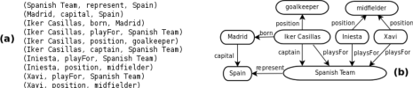
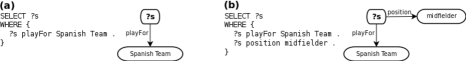
Figure 1: Example of RDF-based modelling.

Figure 2: Examples of (a) SPARQL triple pattern and (b) SPARQL basic graph pattern.

SPARQL (?) is the W3C Recommendation for querying RDF. It is a graph-matching language built on top of triple patterns, that is, RDF triples in which each subject, predicate or object may be a variable. This means, that eight different triple patterns are possible in SPARQL (variables are preceded, in the pattern, by the symbol ?): (S,P,O), (S,?P,O), (S,P,?O), (S,?P,?O), (?S,P,O), (?S,?P,O), (?S,P,?O), and (?S,?P,?O).

SPARQL builds more complex queries (generically referred to as Basic Graph Patterns: BGPs) by joining sets of triple patterns. Thus, competitive SPARQL engines require, at least, fast triple pattern resolution and efficient join methods. Additionally, query optimizers are required to build efficient execution plans that minimize the amount of intermediate results to be joined in the BGP. Query optimization is orthogonal to the current work, and any existing technique can be implemented on top of k²-triples.

Figure 2 shows two simple SPARQL queries over the RDF excerpt described in the example above:

• The first query (left), expressed in normative SPARQL syntax on the left of the figure, represents the triple pattern (?S,P,O). It asks for all subjects related to the Spanish Team through the predicate playFor. From a structural perspective (bottom), this query is a subgraph comprising two nodes connected through the edge labeled playFor: the destination node represents the element Spanish Team, whereas the source node is a variable. This way, the query resolution involves graph pattern matching for locating all nodes that can play the source role in this query subgraph. In this case, the valid nodes represent the players Iker Casillas, Iniesta, and Xavi.

• The second query restricts the previous one for only retrieving the midfielder players of the Spanish Team. This refinement is implemented through a second triple pattern (?S,P,O) setting the predicate position and the object midfielder. As can be seen on the right figure, the two triple patterns of the query are joined by their subject. Its resolution matches the query subgraph to the RDF graph, and retrieves the elements conforming to the variable node; in this case, the result contains the players Iniesta and Xavi.

RDF is defined as a logical data model, so no restrictions are posed on its physical representation and/or storage. However, its implementation has a clear effect on the retrieval efficiency, and therefore on the success of a SPARQL engine within an RDF store. We review below the existing techniques for modeling, partitioning, and indexing RDF, and discuss their use in some real RDF stores. Our goal is to show the achievements and shortcomings in the state of the art to highlight the potential for improvement on which our work focuses. We firslty show the approaches based on a relational infrastructure, and then the solutions natively designed for handling RDF.

2.1 Relational Solutions

Some logical schemes have been proposed for representing RDF over the infrastructure provided by relational databases, but their success has been limited due to the strictness of the relational model for handling the semi-structured RDF features. Nevertheless, there is still room for optimization in the field of relational solutions for RDF management (?), and we describe below the most used schemes.

Single three-column table

This is the most straightforward scheme for modelling RDF over relational infrastructure. It represents RDF triples as generic tuples in a huge three-column table, so generic BGP resolution involves many expensive self-joins on this table. Systems such as 3store (?) or the popular Virtuoso implement this scheme.

Property tables

This model arises as a more practical scheme for RDF organization in relational databases because it proposes to create relational-like property tables out of RDF data. These tables gather together information about multiple predicates (properties) over a list of subjects. Thus, a given property table has many columns as different predicates (one per column) are used for describing the subjects that it stores (in rows). Although this model reduces significantly the number of self-joins, the cost of the query resolution remains high. Besides, the use of property tables induces two additional problems. On the one hand, storage requirements increase because NULL values must be explicitly stored, in each tuple, if the represented subject is not described for a given property in the table. On the other hand, multi-valued attributes are abundant in semantic datasets and they are somewhat awkward to express in property tables (?). Thus, property tables are a competitive choice for representing well-structured datasets, but they lose potential in a general case. Systems like Jena (?) or Sesame (?) use property tables for modeling RDF.

Vertical partitioning

The vertical partitioning (VP) scheme (?) can be seen as a specialized case of property tables in which each table gathers information about a single predicate. This way, VP uses many tables as different predicates are used in the dataset, each one storing tuples (S,O) that represent all (subject,object) pairs related through a given predicate. Each table is sorted by the subject column, in general, so particular subjects can be located quickly, and fast merge joins can be used to reconstruct information about multiple properties for subsets of subjects (?). However, this decision penalizes queries by object that require additional object indexing for achieving competitive resolution.

VP-based solutions avoid the weaknesses previously reported for property tables because only non-NULL values are stored, and multi-valued attributes are listed as successive tuples in the corresponding table. However, VP-based solutions suffer from an important lack of efficiency for resolving queries with unbounded predicate; in this case, all tables must firstly be queried and their results must then be merged to obtain the final result. This cost increases linearly with the number of different predicates used in the dataset, so VP is not the best choice for representing datasets with many predicates.

Abadi, et al. (?; ?) report that querying performance in column-oriented databases is up to one order of magnitude better than that obtained in row-oriented ones. This fact motivates the implementation of their system SW-Store as an extension of the column-oriented database C-Store (?). SW-Store leverages all the advantages reported above, but also suffers from a lack of scalability for queries with unbounded predicate. SW-Store, like some other approaches (such as the reviewed below: Hexastore, RDF3X, and BitMat), firstly perform a dictionary encoding that maps long URIs and literal values to integer IDs. This decision allows triples to be rewritten as three-ID groups, and this is the representation finally stored in the database. Sidirourgos, et al. (?) show additional experiments on VP. They replace C-Store by MonetDB in the database layer; these systems show a couple of differences (?): i) data processing in C-Store is disk-based while it is memory-based in MonetDB; and ii) C-Store implements carefully optimized merge joins and makes heavy use of them, whereas MonetDB uses merge joins less frequently. Even so, MonetDB arises as a competitive choice in this scenario (?).

2.2 Native Solutions

Native solutions are custom designed from scratch to better address RDF peculiarities. Although some works (?; ?; ?) propose different graph-based models, the main line of research focuses on multi-indexing solutions. Harth and Decker (?) propose a six-index structure for managing quads. This scheme allows all quads conforming to a given query pattern (in which the context can also be a variable) to be quickly retrieved. This experience has been integrated in some systems within the current state of the art for RDF management.

Hexastore

(?) It adopts the rationale of VP and multi-indexing, but takes it further, to its logical conclusion. In contrast to VP, Hexastore treats subjects, predicates, and objects equally. That is, whereas VP prioritizes predicates and indexes pairs (subject,object) around them, Hexastore builds specific indexes around each dimension and defines a prioritization between the other two:

• For each subject S, two representations (P,O) and (O,P) are built.

• For each predicate P, two representations (S,O) and (O,S) are built.

• For each object O, two representations (S,P) and (P,S) are built.

This way, Hexastore manages six indexes: (S,P,O), (S,O,P), (P,S,O), (P,O,S), (O,S,P), and (O,P,S). In a naive comparison, the VP scheme (sorted by subject) can be seen as an equivalent representation to the index (S,P,O) in Hexastore. Thus, Hexastore stores triples in a combination of sorted sequences that requires, in the worst case, 5 times the space used to index the full dataset in a single triples table. This is because some sequences can be shared between different indexes (for instance, the object sequence is interchangeably used in the indexes SPO and PSO). The Hexastore organization ensures primitive resolution for all triple patterns and also that the first step in pairwise joins can be always implemented as fast merge joins. However, its large storage requirements slow down Hexastore when representing large datasets, because it is implemented as an in-memory solution.

RDF3X

(?) It goes one step further and introduces index compression to reduce the spatial requirements reported above. In contrast to Hexastore, RDF3X creates its indexes over a single “giant triples table” (with columns v₁,v₂,v₃), and stores them in a (compressed) clustered B⁺-tree. Triples, within each index, are lexicographically sorted allowing SPARQL patterns to be converted into range scans.

The collation order implemented in the RDF3X table causes neighboring triples to be very similar. In most cases, neighboring triples share the values in v₁ and v₂, and the increases in v₃ are very small. This fact facilitates differential compression to represent a given triple with respect to the previous one. This scheme is leaf-oriented within the B⁺-tree, so the compression is individually applied on each leaf. Although the authors test some well-known bitwise codes ($\gamma$-codes, $\delta$-codes, and Golomb codes (?)), they finally apply a bytewise code specifically designed for diferential triples compression. This technique ensures highly-efficient decompression with a slight spatial overhead with respect to the most effective codes. Finally, it is worth noting that RDF3X also manages aggregated indexes (SP), (PS), (SO), (OS), (PO), and (OP), which store the number of ocurrences of each pair in the dataset. RDF3X also contributes with a RISC-style query processor that mainly relies on merge joins over the sorted indexes. Besides, it implements a query optimizer mostly focused on join ordering in its generation of execution plans.

RDF3X reports a very efficient performance that outperforms SW-Store by a large margin. These results make it a leading reference in the area. However, despite its compression achievements, the spatial requirements in RDF3X remain very high. This involves an indirect overhead to the querying performance because large amounts of data need to be transferred from disk to memory, and this can be a very expensive process with respect to the query resolution itself (?; ?).

BitMat

(?) It follows the idea of managing compressed indexes, but it goes another step further and proposes querying algorithms that directly perform on the compressed representation. BitMat introduces an innovative compressed bit-matrix to represent the RDF structure. It is conceptually designed as a bit-cube S$\times$P$\times$O, but its final implementation slices to get two-dimensional matrices: SO and OS for each predicate P, PO for each subject S, and PS for each object O. These matrices are run-length (?) compressed by taking advantage of their sparseness. Two additional bitarrays are used to mark non-empty rows and columns in the bitmats SO and OS. The results reported for BitMat show that it only overcomes the state of the art for low selectivity queries. However, it is an interesting achievement because it demonstrates that avoiding materializaton of intermediate results is a very significative optimization for these queries.

Finally, hybrid (?) and full in-memory stores (?; ?) represent an emerging alternative in this scenario, but their current results are limited for managing small datasets, as previously shown for Hexastore. Their scalability is clearly compromised by the use of structures, like indexes and hash tables, that demand large amounts of memory. However, some semantic applications, such as inference-based ones, claim for scalable in-memory stores because they perform orders of magnitude faster if the entire dataset is in memory (?), and they also support a higher degree of reasoning. New opportunities arise for in-memory stores thanks to the advances in distributed computing. This class of solutions, recently studied (?; ?) on the MapReduce framework, allows arbitrarily large RDF data to be handled in main memory because more nodes can be added to a cluster when more resources were necessary. However, these systems still require further research to ensure efficient RDF exchanging (?; ?), as well as efficient performance in each node.

3 Succinct Data Structures

Succinct data structures (?) aim at representing data (e.g., sets, trees, hash tables, graphs, texts) using as little space as possible. They are able to approach the information theoretic minimum space required to store the original data, but also retain direct access to the data. These features yield competitive overall performance, because they can implement specific functionality in faster levels of the memory hierarchy due to the spatial reductions obtained. This section covers the basic concepts about the succinct data structures involved in our approach.

3.1 Binary Sequences

Binary sequences (bitstrings) are the basis of many succinct data structures. A bitstring $\mathcal{B}[1,n]$ stores a sequence of $n$ bits and must provide efficient resolution for three basic operations:

• rank${}_{a}(\mathcal{B},i)$ counts the occurrences of the bit $a$ in $\mathcal{B}[1,i]$.

• select${}_{a}(\mathcal{B},i)$ locates the position for the $i$-th occurence of $a$ in $\mathcal{B}$.

• access$(\mathcal{B},i)$ returns the bit stored in $\mathcal{B}[i]$.

All these operations can be resolved in constant time using $n+o(n)$ bits of total space: $n$ bits for $\mathcal{B}$ itself, and $o(n)$ additional bits for the structures used to answer the queries. In this paper, we consider an implementation (?) which uses, in practice, $5\%$ extra space on top of the original bitstring size and provides fast query resolution.

3.2 Directly Addressable Codes (DACs)

The use of variable-length codes is the basic principle of data compression: the most frequent symbols are encoded with shorter codewords, whereas longer codewords are used for representing less frequent symbols. However, variable-length codes complicate random access to elements in the compressed sequence, which is required in many practical scenarios (as those studied in this paper) for efficient retrieval. Directly Addressable Codes (DACs) (?; ?) are a practical solution to this problem.

DACs start from a variable-length encoding of the symbols in a sequence. Each codeword (a variable-length bit sequence) is accommodated in a number of fixed-length chunks, using as many chunks as necessary, and thus the encoded sequence can be regarded as a sequence of chunks. This sequence is rearranged in several levels: the first one concatenates the first chunk of all the codewods in the sequence, the second level concatenates the second chunk of all codewords of length more than one, and so on until the chunks of the longest codewords are processed. Two structures are used for representing the information in each level: an array $\mathcal{A}$ concatenates the chunks corresponding to this level, and a bistring $\mathcal{B}$, which stores one bit for each element in $\mathcal{A}$, indicates whether each chunk is the last within its codeword.

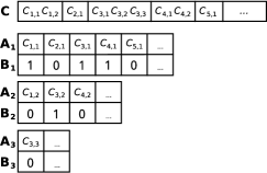
Figure 3: Example of the DAC-based representation of the sequence $\mathcal{C}$.

Example 3.1.

Figure 3 illustrates this reorganization. The compressed sequence $\mathcal{C}$ comprises five symbols: the first one is encoded with a 2-chunk codeword ($\mathcal{C}_{1,1}$, $\mathcal{C}_{1,2}$), the second one with a 1-chunk codeword ($\mathcal{C}_{2,1}$), and so on. The first DAC level stores in $\mathcal{A}_{1}$ all the first chunks of the codewords in $\mathcal{C}$: $[\mathcal{C}_{1,1},\mathcal{C}_{2,1},\mathcal{C}_{3,1},\mathcal{C}_{4,1},\mathcal{C}_{5,1}]$, whereas the bitstring $\mathcal{B}_{1}$ list all corresponding bits: $[10110]$. As can be seen, 0-bits indicate that the corresponding codewords finish in the current level (the second and the fifth codewords are fully represented with a single chunk), whereas 1-bits mean that the codewords continue in the next level (the first, third, and fourth codewords are continued in the second level). Thus, the second level represents the second chunks of these codewords: $\mathcal{A}_{2}=[\mathcal{C}_{1,2},\mathcal{C}_{3,2},\mathcal{C}_{4,2}]$, and gives the information about which finish: $[010]$. Finally, the third level encodes the last chunk of the third codeword.

DACs enable direct access to any element in the encoded sequence. To access the codeword at position $i=i_{1}$, $\mathcal{B}_{1}[i_{1}]$ is firstly checked. If $\mathcal{B}_{1}[i_{1}]=0$, this is the last chunk and the value is fully represented in the current level, so $\mathcal{C}[i]=\mathcal{A}_{1}[i_{1}]$. Otherwise ($\mathcal{B}_{1}[i_{1}]=1$), the following chunks must be fetched. The codeword is continued in the position $i_{2}=rank_{1}(\mathcal{B},i_{1})$ of the second level. As before, the bitstring is firstly checked: if $\mathcal{B}_{2}[i_{2}]=0$, this is the last chunk. In this case, the codeword value is obtained as $\mathcal{C}[i]=\mathcal{A}_{1}[i_{1}]+\mathcal{A}_{2}[i_{2}]\textperiodcentered 2^{b}$, where $b$ is the chunk length (in bits). If $\mathcal{B}_{2}[i_{2}]=1$, the process continues iteratively until the codeword is fully extracted.

Accessing a codeword in a DAC compressed sequence takes $O(\log(M)/b)$ time in the worst case, where $M$ is the longest codeword length. However, this access time is lower for elements with shorter codewords, and these are the most frequent ones.

3.3 K²-trees

The k²-tree (?; ?) is a succinct data structure for graph representation. It models a graph of $n$ vertices through its (binary) adjacency matrix, $\mathcal{M}$, of size $n\times n$. Thus, $\mathcal{M}[i,j]=1$ iff the vertices represented in the $i$-th row and the $j$-th column are related.

The k²-tree leverages sparseness and clustering features, which arise in some classes of real-world graphs (such as Web graphs (?) and social networks (?)), to achieve compression. These features imply the existence of large “empty” areas (all cells have value 0), and the k²-tree excels at compressing them. Conceptually, the k²-tree subdivides the matrix into $k^{2}$ sub-matrices of the same size, which results in $k$ rows and $k$ columns of sub-matrices of size $n^{2}/k^{2}$. Each of those $k^{2}$ sub-matrices is represented in the tree using a single bit that is appended as a child of the root: a bit 1 is used for representing those sub-matrices containing at least one cell with value $1$, whereas a 0-bit means that all cells in the corresponding sub-matrix are $0$. Once this first level is built, the method proceeds recursively for each child with value $1$ until sub-matrices full of 0s or the last level of the tree are reached. This process results in a non-balanced k²-ary tree in which the bits in its last level correspond to the cell values in the original matrix. If the number of rows and columns in the adjacency matrix is not a power of $k$, the matrix is expanded to the right and bottom with 0s, obtaining an extended matrix of size $n^{\prime}\times n^{\prime},n^{\prime}=k^{\lceil\log_{k}n\rceil}$. This expansion causes just a little overhead because of the $k^{2}$-tree ability to compress the large areas of 0s created after the expansion.

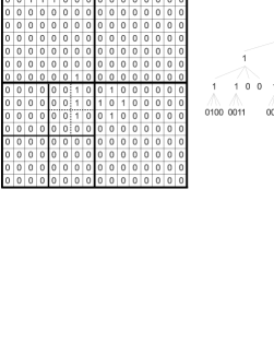
Figure 4: Example of k²-tree for an adjacency matrix of size $16\times 16$.

The k²-tree is implemented in a very compact way using two bitstrings: T (tree) and L (leaves). T stores all the bits in the k²-tree except those stored in the last level. The bits are placed following a levelwise traversal: first the k² binary values of the children of the root node, then the values of the second level, and so on. This configuration enables the k²-tree to be traversed by performing efficient rank and select operations on the bitstring. On the other hand, L stores the last level of the tree, comprising the cell values in the original matrix. Although L was originally devised to be implemented with a bistring, a recent improvement stops the decomposition when the matrices reach size $k_{L}\times k_{L}$ and uses DACs to compress them according to frequency while retaining fast direct access to any leaf sub-matrix (?).

Besides of its compression ability, the k²-tree provides various navigational operations on the graph. In particular, for a given vertex $v$, the k²-tree supports the operations of retrieving $(i)$ all the vertices pointed by $v$ (direct neighbors), and $(ii)$ all the vertices that point to $v$ (inverse neighbors). Additionally, range queries (retrieving all the connections within a sub-matrix), and the fast check of a given cell value are also supported by the k²-tree.

Conceptually, direct neighbors retrieval, for a vertex $v_{i}$, requires finding all the cells with value $1$ in the $i$-th row. Symmetrically, the inverse neighbors of $v_{i}$ are retrieved by locating all the 1s in the $i$-th column. Both operations are efficiently implemented on a top-down traversal of the tree, requiring O(1) time per node visited (and $O(n)$ overall time in the worst-case, but possibly less in practice). This traversal starts at the root of the k²-tree, $pos=0$, and visits in each step the children of all nodes with value 1 in the previous level and whose matrix area is not disjoint from the area one wants to retrieve. Given a node, represented at the position $pos_{i}$ of T, its $k^{2}$ children are represented consecutively from the position $pos_{i}=rank_{1}(T,pos)\cdot k^{2}$ of T:L.

Example 3.2.

Figure 4 shows a $16\times 16$ adjacency matrix (left) and the k²-tree (right) representing it, using $k=2$. The configurations for the the two bitstrings, T and L, implementing the k²-tree, are also shown at the bottom of the figure. The matrix is conceptually divided into $2^{2}=4$ sub-matrices. In the first step, the sub-matrices are of size $8\times 8$. Assume we are interested in retrieving the direct neighbors of the $11$-th vertex, so we need to find all the cells with value $1$ in the $11$-th row of the adjacency matrix. The first step starts at the root of the k²-tree, $pos=0$, and computes the children overlapping the eleventh row. These are the third and the fourth children (representing the sub-matrices at the bottom of the original adjacency matrix), and these are respectively represented in $\mathbf{T}[2]$ and $\mathbf{T}[3]$ (assuming that positions in T are numbered from 0). In both cases, $\mathbf{T}[2]$ and $\mathbf{T}[3]$ have value 1, so both children must be traversed. For simplicity we only detail the procedure for the third child, so now $pos=2$. The second step first computes the position representing the first child of the current vertex: $pos=rank_{1}(\mathbf{T},2)\cdot 2^{2}=2\cdot 4=8$, and checks the value of the $k^{2}=4$ bits stored from $\mathbf{T}[8]$: $[0100]$. In this case, only the second child (represented at $pos=9$) has value 1, so this is the node to be visited in the third step. The children for this node are located from $pos=rank_{1}(\mathbf{T},9)\cdot 2^{2}=7\cdot 4=28$, and contain values $[0101]$. Although the second child is 1, this is not a valid match for our query because it has no intersection with the $11$-th row. This means that only the fourth child (represented at $pos=31$) is visited in the fourth step. The new position $pos=rank_{1}(\mathbf{T},31)\cdot 2^{2}=14\cdot 4=56$ is larger than $|\mathbf{T}|=36$, so it represents a leaf. Thus, the $k^{2}$ resulting leaves must be checked from position $56-36=20$ of L. The bits $[1000]$ represent this submatrix, so one connection is found for the $11$-th row, and it is the $7$-th column.

Similar algorithms implement the extended functionality. Checking the value of a given cell also uses a recursive descent, but it only visits the single appropiate child, in each level, for the given query. Range queries are performed similarly, but each step visits all the children representing the rows and columns involved in the query. More details about both algorithms can be found in (?).

4 Full-In-Memory Vertical Partitioning on k²-triples

This section describes how the k²-tree structure can be applied to the problem of RDF storage. Our approach is called k²-triples. We firstly perform a specific dictionary encoding that allows triples to be managed as three-ID groups: $(id_{1},id_{2},id_{3})$, in which $id_{1}$ is the integer value that identifies the subject in the dictionary, $id_{2}$ identifies the predicate, and finally $id_{3}$ identifies the object. This decision simplifies data partitioning on k²-trees because a direct correspondence can be established between rows and columns in the adjacency matrix and subject and object IDs in the dictionary.

4.1 Dictionary Encoding

Dictionary encoding is a common preliminary step performed before data partitioning. All different terms used in the dataset are firslty extracted from the dataset and mapped to integer values through a dictionary function. As explained above, this allows long terms occurring in the RDF triples to be replaced by short IDs referencing them within the dictionary. This simple decision greatly compacts the dataset representation, and mitigates scalability issues.

We propose a dictionary organization comprising four independent categories, in which terms are usually organized in lexicographic order (?; ?; ?):

• Common subjects and objects (SO) organizes all the terms that play both subject and object roles in the dataset. They are mapped to the range [1, $|$SO$|$].

• Subjects (S) organizes all the subjects that do not play an object role. They are mapped to [$|$SO$|$+1, $|$SO$|$+$|$S$|$].

• Objects (O) organizes all the objects that do not play a subject role. They are mapped to [$|$SO$|$+1, $|$SO$|$+$|$O$|$]. Note this interval overlaps with that for S, since confusion cannot arise.

• Predicates (P) maps all the predicates to [1,$|$P$|$].

In this way, terms playing subject and object roles are represented only once. Moreover, the intervals for subjects and objects are contiguous. This decision, on the one hand, provides a dictionary size reduction as it prevents the duplicate representation of these terms. This is a significant reduction if we consider that up to $60\%$ of the terms in the dictionary are in the SO area for real-world datasets (?). On the other hand, this four-category organization improves performance for subject-object joins because all their possible matches are elements playing both subject and object roles, and all of them are in the range [1, $|$SO$|$]. Thus, this join resolution is concentrated on the area of SO and avoids querying for the remaining subjects and objects.

How the dictionary is finally implemented is orthogonal to the problem addressed in this paper, and any existing technique within the state of the art could be adapted for managing our organization. Nevertheless, we emphasize that RDF dictionaries take up to 3 times more space than that required for representing the triples structure (?), so compressed dictionary indexes are highly desirable for efficient and scalable management of huge RDF datasets.

Example 4.1.

Figure 5 illustrates our dictionary organization over the RDF excerpt used in Figure 2. As can be seen, the terms Madrid and Spanish Team (playing as subject and object) are respectively identified with the values 1 and 2, the three subjects are represented in the range [3,5], and equally the three objects are identified with the same values: {3,4,5}. Finally, the six predicates used in the example are identified in the range [1,6]. On the right of the figure, the ID-based representation of the original triples is shown.

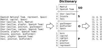
Figure 5: Example of dictionary encoding on k²-triples.

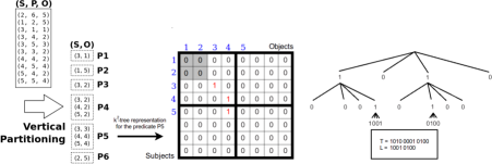
Figure 6: Vertical Partitioning on k²-triples (the parameter $k$ is set to 2).

4.2 Data Partitioning

k²-triples models RDF data following the well-known vertical partitioning approach. This scheme reorganizes a dataset into $|$P$|$ disjoint subsets that contain all the triples related to a given predicate. Thus, all triples in a subset can be rewritten as pairs of subject and object (S,O), because the corresponding predicate is implicitly associated to the given subset.

Each subset is independently indexed in a single k²-tree that represents subjects and objects as rows and columns of the underlying matrix. That is, each k²-tree models an adjacency matrix of $|$SO$|+|$S$|$ rows and $|$SO$|+|$O$|$ columns. In practice, as commented above, the k²-tree is extended to the next power of $k$ to obtain a square matrix of size $n^{\prime}\times n^{\prime},n^{\prime}=k^{\lceil\log_{k}(|SO|+\max(|S|,|O|))\rceil}$.

Finally, it is worth noting that all the k²-trees used in our approach are physically built with a hybrid policy that uses value $k=4$ up to the level $5$ of the tree, and then $k=2$ for the rest (?; ?). The leaves, regarded as submatrices of size $8\times 8$, are encoded using DACs (?; ?).

Example 4.2.

Figure 6 (left) shows the vertical partitioning of our excerpt of RDF. As can be seen, six different subsets are obtained (one for each different predicate), and the triples are rewritten as pairs (S,O) within them. For example, the triples for the predicate 5: (3,5,3), (4,5,4), (5,5,4), are rewritten as pairs: (3,3), (4,4), (5,4), and they are then managed within the subset P5 associated to the predicate 5.

The right side of the figure shows the adjacency matrix underlying to the k²-tree used for representing the subset P5. The shadow cells are the area SO in which elements playing as subjects and nodes are represented. Note that only the first five rows (for the five existing subjects) and the five first columns (for the five existing objects) are really used, hence all the triples are stored in these ranges. In this case, 1-bits are found in the cells (3,3), (4,4), (5,4) in which the triples (3,5,3), (4,5,4), (5,5,4) are represented. As can be seen, the resulting matrix contains a very sparse distribution of 1-bits, and this is the best scenario for k²-trees because of their ability to compress large empty areas.

4.3 Indexing Predicates for Subjects (SP) and Objects (OP)

The resolution of queries involving variable predicates is the main weakness of systems that implement vertical partitioning. In our case, all k²-trees must be traversed for resolving triple patterns with unbounded predicate (see next section). This is hardly scalable when a large number of predicates is used in the dataset. In this section, we enhance k²-Triples in order to minimize the number of k²-trees that must be traversed for resolving triple patterns involving variable predicates.

The triple pattern classification, given in Section 2, shows that (?S,?P,?O) is the only pattern with unbounded predicate that provides neither value for the subject nor the object. However, this pattern always scans the full dataset to retrieve all the triples within it, and no specific optimizations are possible for it. Thus, we can leverage that subject and/or object values are provided, and use them to optimize the number of k²-trees that must be traversed for resolving the remaining patterns with unbounded predicate. This is achieved through two specific indexes:

• The Subject-Predicate (SP) index organizes the lists of all the different predicates related to each subject in the dataset.

• The Object-Predicate (OP) index organizes the lists of all the different predicates related to each object in the dataset.

Empirical results (?) show that the average size of these lists of predicates for subjects and objects is, at most, one order of magnitude less than the number of total predicates used in real-world datasets. This fact not only ensures a great improvement for queries with unbounded predicate, but also implies a limited additional space for SP and OP indexes. Thus, this enhanced revision of k²-Triples also retains the original aim of obtaining a compact RDF representation.

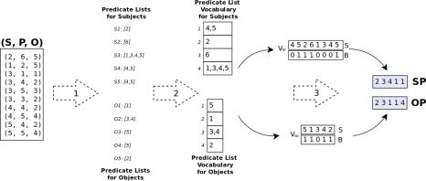
Figure 7: Building SP and OP indexes.

Both SP and OP indexes rely on a compact representation of their predicate lists. The predicate list, for a given subject, organizes all the different predicates related to it. These predicate lists are common for some subjects, and this can be leveraged to achieve space savings. For this purpose, we obtain the set of all the different predicate lists (we referred this set to as the predicate list vocabulary), and sort them according to their frequency. In this way, the predicate lists appearing in more subjects are represented in the first positions of the vocabulary and are encoded with smaller codewords. A similar reasoning applies for objects. We respectively refer to V_sp and V_op as the predicate list vocabularies for subjects and objects.

Example 4.3.

The arrow 1 in Figure 7 shows the predicate lists obtained for the subjects and objects in the RDF excerpt used in the previous examples. As can be seen, the subject 1 is related to a 1-element list containing the predicate 2; the list for the subject 2 contains the element 6; for the subject 3, its predicate list contains four elements: 1,3,4,5; and the subjects 4 and 5 are related to 2-element predicate lists containing the elements 4,5. The arrow 2 illustrates how predicate lists vocabularies are obtained. Let us consider the case of subjects: the list 4,5 is represented in the first position because it is related to two different subjects (4 and 5), whereas the other lists are only related to a single subject. The case of objects is similar: the list 5 is related to the objects 3 and 4, and the remaining lists appear only once.

We propose a succinct vocabulary representation based on the following two structures:

• An integer sequence $\mathcal{S}$ that concatenates all the predicate lists according to their frequency. Thus, the most frequent lists appear at the beginning of the sequence, whereas the least frequent ones are at the end. Each element in $\mathcal{S}$ takes $\log(|\mathtt{P}|)$ bits of space.

• A bitstring $\mathcal{B}$ that delimits and identifies predicate lists within the vocabulary. That is, the $i$-th 1-bit in the position $p$ of the bit sequence means that the predicate list identified as $i$ finishes in the $p$-th position of $\mathcal{S}$.

$\mathcal{B}$ enables efficient list extraction within the vocabulary (let us assume that $\mathtt{select}_{1}(\mathcal{B},0)=1$), because of the $p$-th predicate list is stored in $\mathcal{S}[i,j]$, where $i=\mathtt{select}_{1}(\mathcal{B},p-1)+1$, and $j=\mathtt{select}_{1}(\mathcal{B},p)-1$.

This representation allows the SP and OP indexes to be easily modelled as integer sequences. We detail SP, but the same representation applies to OP. The index SP is modelled as a sequence of integer IDs of length $|\mathcal{S}|$. In this way, the $p$-th value in SP (referred to as $\mathrm{SP}[p]$) contains the ID of the predicate list related to the subject $p$, and it can be extracted from V_sp by using the simple extraction process explained above. The elements of index SP are finally represented using DACs. This retains direct access to any position in the index and also leverages the frequency distribution of predicate lists to achieve compression. Note that DACs assign shorter codewords to smaller integers and these are used for representing the most frequent lists within the vocabulary.

Example 4.4.

The arrow 3, in Figure 7, illustrates the final SP and OP index configurations. As can be seen, SP lists the IDs [2,3,4,1,1]. This means that the first subject is related to the second predicate list, the second subject to the third list, and so on. For instance, if we want to extract the list of predicates related to the subject 3, we firstly retrieve its ID as $\mathrm{SP}[3]=4$. Thus, the fourth list must be extracted from V_sp. This is represented in $\mathcal{S}$ from the position $i=\mathtt{select}_{1}(\mathcal{B},3)+1=4+1=5$ to the position $j=\mathtt{select}_{1}(\mathcal{B},4)=8$, and contains the predicates 1,3,4, and 5.

5 Triple Pattern Resolution over k²-triples

Triple patterns are the basic lookup unit on RDF triples; more complex SPARQL queries can be translated into plans involving triple pattern resolution. Thus, RDF retrieval strongly relies on the performance achieved for triple pattern resolution. This is one of the main strengths of our approach, because k²-triples can answer all patterns on the highly-optimized operations provided by the k²-tree structure:

• (S,P,O) is directly implemented on the operation that checks the value of a given cell in the k²-tree. That is, the triple (S,P,O) is in the dataset iff the cell (S,O) (in the matrix representing the subset of triples associated to the predicate P) contains the bit $1$. This operation returns a boolean value and it is usually required within ASK queries.

• (S,?P,O) generalizes the previous pattern by checking the value of the cell (S,O) in all the k²-trees. The result is an ID-sorted list of all the predicates whose k²-tree contains a 1 in this cell. The process can be sped up by first intersecting the predicate lists of SP and OP respectively associated to S and O, obtaining a list of predicates $\mathtt{P}_{i}$ that contain objects related to S as well as subjects related to O. Then, only the k²-trees of those $\mathtt{P}_{i}$ need be considered for pairs (S,O).

• (S,P,?O) can be seen as a forward navigation from S to all the objects related to it through predicate P. Thus, it is equivalent to a direct neighbors retrieval that locates all the columns with value 1 in the row associated to the subject S within the k²-tree for P. The objects matching the pattern are returned in sorted order.

• (S,?P,?O) generalizes the previous pattern by performing direct neighbor retrieval in all the k²-trees. In this case, the result comprises many ID-sorted lists of objects for the predicates related to S. This is sped up by using the information stored in the SP index. A subject-based query on this SP index returns the predicate list containing all predicates P_i related to the subject S. Thus, direct neighbors retrieval is only performed on the $|$P${}_{i}|$ k²-trees modeling the predicates within the list.

• (?S,P,O) corresponds to a backwards navigation from O to all the subjects related to it through P. This is equivalent to a reverse neighbors retrieval that locates all the rows with value 1 in the columns associated to the object O within the k²-tree for P. The subjects matching the pattern are returned in sorted order.

• (?S,?P,O) generalizes the previous pattern by performing reverse neighbors retrieval in all the k²-trees. In this case, the result comprises many ID-sorted lists of subjects for the predicates related to O. An object-based query on the OP index speeds up the query by restricting the predicate list to those P_j with which object O relates to some subject.

• (?S,P,?O) is equivalent to retrieving all the values 1 in the k²-tree associated to the predicate P. This is easily implemented by a range query performing a full top-down traversal that retrieves all the pairs (S,O) in the structure.

• (?S,?P,?O) generalizes the previous pattern by obtaining all the 1s in all the k²-trees used for representing the predicates in the dataset.

6 Join Resolution over k²-triples

The core of SPARQL relies on the concept of Basic Graph Pattern (BGP), and its semantics to build conjunctive expressions by joining triple patterns through shared variables. BGPs are reordered and partitioned into pairs of triple patterns sharing exactly one variable. Thus, the performance of BGPs is clearly determined by the algorithms available for joining these patterns, and also for the optimization strategies to order the joins. This second topic is orthogonal to this paper and is not addresed.

k²-triples provides subject-subject and object-object join resolution. This overcomes traditional vertical partitioning, which only gives direct support for subject-subject joins, and requires an additional object index for efficient resolution of object-object joins. Besides, k²-triples also supports subject-object joins. These are efficiently implemented by considering only the common area SO in which nodes playing as subjects and objects are exclusively represented. Our native support for cross-joins is a significant improvement with respect to traditional vertical partitioning, in which framework cross-joins are described as rather expensive and inefficient operations (?). This fact is a clear weakness for these traditional solutions because cross-joins are the basis for implementing the common path expressions queries. In (?), the path expression query problem is tackled in a non-general way: the results of only some selected paths are precalculated and stored for their efficient querying. Finally, it is worth noting that operations involving predicates as join variables are underused in practical terms (?).

This section describes the algorithms and mechanisms implemented on k²-triples for join resolution. We firstly classify join operations and then detail the join algorithms implemented by our approach. The section ends with the description of the specific mechanisms provided by k²-triples for resolving each kind of join operation according to our different join algorithms.

6.1 Classifying Join Operations

Figure 8 classifies the join operations according to the classes studied in this section. Although all of them refer to subject-object joins, subject-subject and object-object ones are similarly classified and solved on the same guidelines. We refer to ?X as the join variable in each class.

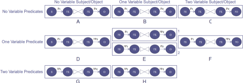
Figure 8: Classification of subject-object joins supported in k²-triples.

Join operations are organized, by rows, according to the state of the predicates in the two patterns involved in the join:

• Row no variable predicates lists the joins in which both triple patterns provide their predicates (classes A, B and C).

• Row one variable predicate lists the joins in which one triple pattern provides its predicate, whereas the other one leaves it variable (classes D, E and F).

• Row two variable predicates lists the joins in which both triple patterns leave as variables their corresponding predicates (classes G and H).

The column-based classification lists join operations according to the state of the nodes in the triple patterns. If we consider that the join variable is represented in two of these nodes, the remaining two determine the classes:

• Column no variable subject/object lists the joins in which the value of the two not joined nodes are provided (classes A, D and G).

• Column one variable subject/object lists the joins in which one triple pattern provides its not joined node, whereas the other one leaves it variable (classes B, E and H). From this perspective, the class E is split into two different subclasses: in E.1, one pattern provides its predicate but leaves variable its node, whereas the other pattern provides the node but leaves as variable its predicate; in E.2, one pattern is full-of-variables (it does not provide neither the node nor the predicate), whereas the other one provides both the node and the predicate.

• Column two variable subject/object lists the joins in which both triple patterns leave as variables their not joined nodes (classes C and F).

It is woth noting that the eventual class I is not studied because joins full-of-variables: (?S,?P₁,?X) (?X,?P₂,?O), are not used in practice.

6.2 Join Algorithms

Join algorithms have been widely studied for relational databases (?), and have been recently reviewed from the perspective of semantic Web databases (?). We gather this experience to propose three join algorithms optimized for performing over k²-triples. We will use a simple notation where $T_{l}$ and $T_{r}$ refer to the left and right triple patterns, respectively, involved in the join.

Chain evaluation

This algorithm relies on the foundations of the traditional index join: it firstly retrieves all the solutions for $T_{l}$, and then each one is used for obtaining all the solutions for $T_{r}$. Our implementation firstly resolves the less expensive pattern (assume it is $T_{l}$), and gathers all the values X_i obtained for the join variable ?X. All these values are then used for replacement in $T_{r}$. Note that some of these values can be duplicated and these must be identified before the replacement. These duplicates may belong to the result of range queries or multiple direct/reverse neighbors. We implement an adaptive sort (?) algorithm that merges the results obtained for each predicate leveraging that these are returned in sorted order.

Independent evaluation

This algorithm implements the well-known merge join: it firstly resolves both triple patterns and then intersects their respective solutions, which come sorted by the join attribute.

Interactive evaluation

This algorithm is strongly inspired on the Sideways Information Passing (SIP) mechanism proposed by Neumann and Weikum (?). SIP passes information on-the-fly between the operands involved in the query in a way that the processing performed in one of them can feed back the other and vice versa. Thus, both triple patterns within the join are interactively evaluated and resolved without materialization of intermediate results. This interactive evaluation is easily implemented in k²-triples by means of a coordinated step-by-step traversal performed on those k²-trees involved in the resolution of each pattern within the join. In the next example only two k²-trees are involved, the join attribute is the subject in both trees, and the predicates and objects are fixed, but all the other combinations can be handled similarly.

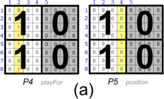
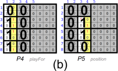
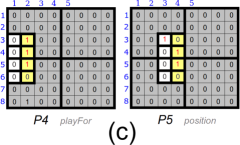
Figure 9: Example of interactive evaluation.

Example 6.1.

Figure 9 illustrates how k²-triples implements the interactive evaluation of the join query shown in Figure 2(b). The original SPARQL query (?X, playFor, Spanish Team) (?X, position, midfielder), is rewritten as (?X, 4,2) (?X,5,4) by performing the ID-based replacement of each term. Thus, the join must be carried out on the k²-trees that respectively model the predicates 4 and 5. Both k²-trees are represented in Figure 9(a). Columns 2 and 4 are respectively remarked for the predicates 4 and 5, since those are the ones we have to join. We consider $k=2$ and the join is implemented as follows:

1. The two matrices $\mathcal{M}_{4}$ and $\mathcal{M}_{5}$ are queried. They are divided into $k^{2}=4$ submatrices (Figure 9(a)). Both right submatrices in both $\mathcal{M}_{4}$ and $\mathcal{M}_{5}$ are discarded because they do not overlap with the columns involved in the current query. The two pairs of left submatrices have value 1, so both may contain results. Thus, we recursively consider the top-left and the bottom-left submatrices of $\mathcal{M}_{4}$ and $\mathcal{M}_{5}$. Note that we could have had to make more than one recursive call per submatrix, had we obtained more than one relevant top or bottom cell in $\mathcal{M}_{4}$ and $\mathcal{M}_{5}$ (not in this case, where the columns are specified).

2. In the top-left submatrices (Figure 9(b)) we discard in turn the right subsubmatrices in $\mathcal{M}_{4}$ and the left subsubmatrices in $\mathcal{M}_{5}$, because they do not intersect the query column. Further, both top subsubmatrices are 0, so we need consider only, recursively, the bottom-left subsubmatrix of $\mathcal{M}_{4}$ paired with the bottom-right subsubmatrix of $\mathcal{M}_{5}$. Similarly, the top-left and top-right subsubmatrices of $\mathcal{M}_{4}$ and $\mathcal{M}_{5}$ are recursively considered on the bottom-left submatrices.

3. The last recursion level (Figure 9(c)) compares leaves in $\mathcal{M}_{4}$ and $\mathcal{M}_{5}$. As in the previous step, we discard the cells that do not overlap with the query columns, and intersect the remaining ones. Three cells are possible results in $\mathcal{M}_{4}$: (3,2), (4,2) and (5,2), so only their corresponding counterparts must be evaluated in $\mathcal{M}_{5}$. Whereas the cell (3,4) has value 0, the other two ones, (4,4) and (5,4), contain 1-bits. Thus, the 4 and 5 represent the subjects in the final query result: Iniesta (4) and Xavi (5).

6.3 Implementing Joins over k²-triples

This section details how k²-triples uses the proposed algorithms for resolving all the join operations classified in Figure 8. We will refer to T_l and T_r as the first and second patterns involved in each class of join. In general, interactive evaluation can be used uniformly on all the cases, whereas chain and independent evaluation can also be used with different strategies depending on the type of join. As a general rule of thumb, chain evaluation is preferable over independent evaluation when the outcome of one side of the join is expected to be much smaller than the other. Interactive evaluation, instead, adapts automatically to perform in the best way on each case. Finally, we remark that we will use indexes SP and OP whenever possible to restrict the set of predicates to consider when the predicate is variable (we will nevertheless remark this when their usage is less obvious).

Joins with no variable predicates

As explained, in these classes of joins both triple patterns provide their predicates. This ensures high performance for interactive resolution because only two parallel k²-tree traversals must be performed. Chain and independent evaluation are also possible, depending on the number of variable nodes involved in each class:

• Joins A. It is the simplest class because only the join variable is not provided. Chain evaluation is advantageous when one operand has much fewer results than the other. Otherwise, independent evaluation is better, as it leverages that both patterns return their results in sorted order.

• Joins B. This class leaves as variable a non-joined node. The subject node of T_l is variable in the example: (?S,P₁,?X) (?X,P₂,O). Chain evaluation is well-suited for this class because it firstly resolves T_r, obtains all the values X_i for ?X, and finally replaces them in T_l. In this way, T_l is trasformed into a group of patterns in which ?X is replaced by each X_i retrieved from T_r. The final result comprises the union of all the results retrieved for the group of patterns obtained from T_l. Nevertheless, independent evaluation also applies for this class. On the one hand, T_r is resolved through a reverse neighbors query, which returns its results in order. On the other hand, a range query returns all results for T_l, which must then be sorted by X. The results of both operations are finally intersected producing the join result set.

• Joins C. Both patterns in the join leave as variables their non-joined nodes. Chain resolution firstly resolves the pattern containing the less frequent predicate (i.e., containing fewer (S,O) pairs), extracts all its pairs, and all their distinct X_i components are then replaced in the other pattern (note we must remove duplicates in the X_i list before replacing each in T_r). Then all the objects found in T_r for each X_i are matched with all the subjects found in T_l for the same X_i. Alternatively, independent evaluation generates all the pairs from both operands, sorted by the ?X component in each case, and intersects the sorted lists.

Joins with one variable predicate

These classes comprise a triple pattern providing its predicate, and another that leaves it variable. In this case, interactive resolution traverses, in parallel, the k²-tree associated to the given predicate, and the $preds$ different k²-trees involved in the other triple pattern resolution. In each recursive step, only a subset of the $preds$ k²-trees stay active for the corresponding submatrix. Chain and independent evaluation strategies are also possible depending on the number of variable nodes involved in each operand:

• Joins D. This class, like Joins A, provides the two non-joined nodes but includes a variable predicate (say, that of T_r). In this case, chain evaluation firstly resolves T_l, obtains all the values X_i for ?X, and finally replaces them in T_r for its resolution, which becomes a set of access to single cell queries. Independent evaluation is also practical. First, T_l is efficiently resolved with a direct neighbors query and its results are retrieved in order. Second, T_r performs $preds$ inverse neighbor queries to obtain the result set for (?X,?P,O), which must be adaptively sorted (for grouping the X_j values) before the final intersection. Note that not only the OP index can be used to restrict the predicates of T_r to those related to O, but we can also restrict using SP to the union of all the X_i values.

• Joins E. This class is split into two subclasses according to the pattern that contains the unbounded predicate and the variable non-joined node.

  • E.1. Chain evaluation can choose between two strategies, depending on which starts with the smaller set of candidates. On the one hand, T_r, which contains the unbounded predicate and provides the non-variable node, can be firstly resolved and its results be adaptively sorted to remove duplicates. These results X_j for ?X are then replaced in T_l for its final resolution using inverse neighbor queries. On the other hand, we could collect all the (S,X_i) pairs from P₁, remove duplicates in X_i, and run access to single cell queries on all the qualifying k²-trees for T_r. Independet evaluation is also possible, much as done for Join D operations.

  • E.2. Chain evaluation firstly resolves T_r and all their bindings X_j for ?X are then used for replacement in T_l (which is full-of-variables in this case) using $preds$ inverse neighbor queries.

• Joins F. In this class, T_l only provides the predicate, and T_r is full of variables. Chain evaluation firstly resolves T_l, filters duplicate X_i values, and these are finally used for resolving T_r. This last step is restricted using index SP.

Joins with two variable predicates

The triple patterns in this class leave their two predicates as variables. This means that interactive resolution traverses in parallel all the different k²-trees involved in each pattern resolution. Chain and independent evaluation can proceed as follows.

• Joins G. This class provides the non-joined nodes and leaves the predicates as variables. Chain evaluation firstly resolves T_l, its bindings for ?X are cleaned from duplicates, and these are finally replaced in T_r for its resolution. Independent evaluation is also suitable. It retrieves the results for each pattern sorted by their ?X component, and then intersects the sorted lists.

• Joins H. In this case, T_l is full of variables and T_r binds the non-joined node. Chain evaluation firstly resolves T_r and its results, clean from duplicates, are used for T_l resolution.

Table 1: Summary of joins resolution in k²-triples (^∗ means that removing duplicates is required for join resolution)

Join	Example	Chain	Inde-	Interactive
Class			pendent	Tl	Tr
A	(S,P1,?X)(?X,P2,O)	Tl $\rightarrow$ Tr	$\surd$	Direct	Reverse
		Tr $\rightarrow$ Tl
B	(?S,P1,?X)(?X,P2,O)	Tr $\rightarrow$ Tl	$\surd^{*}$	Range	Reverse
C	(?S,P1,?X)(?X,P2,?O)	T${}_{l}^{*}$ $\rightarrow$ Tr	$\surd^{*}$	Range	Range
		T${}_{r}^{*}$ $\rightarrow$ Tl
D	(S,P1,?X)(?X,?P2,O)	Tl $\rightarrow$ Tr	$\surd^{*}$	Direct	Reverse ($\times preds$)
E.1	(?S,P1,?X)(?X,?P2,O)	T${}_{l}^{*}$ $\rightarrow$ Tr	$\surd^{*}$	Range	Reverse ($\times preds$)
		T${}_{r}^{*}$ $\rightarrow$ Tl
E.2	(?S,?P1,?X)(?X,P2,O)	Tr $\rightarrow$ Tl		Range ($\times preds$)	Reverse
F	(?S,P1,?X)(?X,?P2,?O)	T${}_{l}^{*}$ $\rightarrow$Tr		Range	Range ($\times preds$)
G	(S,?P1,?X)(?X,?P2,O)	T${}_{l}^{*}$ $\rightarrow$ Tr	$\surd^{*}$	Direct ($\times preds$)	Reverse ($\times preds$)
		T${}_{r}^{*}$ $\rightarrow$ Tl
H	(?S,?P1,?X)(?X,?P2,O)	T${}_{r}^{*}$ $\rightarrow$ Tl		Range ($\times preds$)	Reverse ($\times preds$)

Table 1 summarizes all presented choices for each class of join. The first column indicates the class of join and the second column illustrates a representative of the corresponding class. Column chain evaluation describes how this join strategy is carried out, that is, T_l $\rightarrow$ T_r means that T_l is firstly executed and its results are used for T_r resolution, and vice versa. Column independent evaluation indicates the classes where this strategy can be efficiently used. Finally, column interactive evaluation indicates the k²-tree operations interactively performed for resolving each triple pattern in the join. We indicate with “$\times preds$” the cases where interactive operations involve unbounded predicates.

7 Experimentation

This section studies the performance of k²-triples on a heterogeneous experimental setup comprising real-world RDF datasets from different areas of knowledge. We study both compression effectiveness and querying performance, and compare these results with respect to a consistent set of techniques from the state of the art.

7.1 Experimental Setup

We run experiments on an AMD-Phenom™-II X4 955@3.2 GHz, quad-core (4 cores - 4 siblings: 1 thread per core), 8GB DDR2@800MHz, running Ubuntu 9.10. We built two prototypes:

• k²-triples, the vertical partitioning on k²-trees without the SP and OP indexes.

• k²-triples⁺, which enhances the basic vertical partitioning model with the indexes SP and OP.

Both prototypes were developed in C, and compiled using gcc (version 4.4.1) with optimization -O9.

RDF Stores

We compare our results with respect to three representative techniques in the state of the art (Section 2):

• A vertical partitioning solution following the approach of (?). We implement it over MonetDB because it achieves better performance than the original C-Store based solution (?).

• A memory-based system implemented over Hexastore.

• A highly-efficient store: RDF3X, which was recently reported as the fastest RDF store (?).

All these techniques had been tested following the configurations and parameterizations provided in their original sources.

RDF Datasets

We design a heterogeneous RDF data test comprising four datasets from different areas of knowledge. We use it for testing k²-triples with respect to different data distributions, showing that our approach is competitive in a general scenario. The chosen datasets are the following:

• jamendo is a repository of Creative Commons licensed music.

• dblp provides information on Computer Science journals and proceedings.

• geonames is a geographical database covering all countries and containing a large number of placenames.

• dbpedia is the semantic evolution of Wikipedia, so it is an encyclopedic dataset. dbpedia is considered the “nucleus for a Web of Data” (?).

Table 2: Statistical dataset description

Dataset	Size (MB)	# Triples	# Predicates	# Subjects	# Objects
jamendo	144.18	1,049,639	28	335,926	440,604
dblp	7,580.99	46,597,620	27	2,840,639	19,639,731
geonames	12,347.70	112,235,492	26	8,147,136	41,111,569
dbpedia	33,912.71	232,542,405	39,672	18,425,128	65,200,769

The main statistics of these datasets are described in Table 2. Note that some of the datasets contained duplicated triples, which have been deleted, hence sizes have been updated consequently. As can be seen, different sizes are chosen for overall scalability measurements. In addition, dbpedia lets us analyze how k²-triples perform when the number of predicates increases. It is worth remembering that queries with unbounded predicate are poorly resolved using traditional solutions based on vertical partitioning.

Queries

We design experiments focused on demonstrating the retrieval ability of all RDF stores included in our setup. First, we run triple pattern queries to analyze basic lookup performance. These results feed back join experiments which, in turn, predict the core performance for BGP resolution in SPARQL.

We design a testbed of randomly generated queries covering the entire spectrum of triple patterns and joins. For each dataset, we consider 500 random triple patterns of each type. Note that in all datasets, except for dbpedia, the triple pattern (?S,P,?O) is limited by the number of different predicates.

Join tests are generated by following the aforementioned classification (A-H) (as shown in Figure 8 for Subject-Object joins), and for each one we obtain specific joins Subject-Object (SO), Subject-Subject (SS), and Object-Object (OO). We generate 500 random queries of each join and perform a big-small consideration according to the number of intermediate results: for each join we take the product of the number of results for the first triple pattern and the results of the second triple pattern in the join. Given the mean of this product, we randomly choose 25 queries with a number of intermediate results over the mean (joins big) and other 25 queries with fewer results than the mean (joins small).

We design two evaluation scenarios to analyze how I/O transactions penalize on-disk RDF stores included in our setup. On the one hand, the warm evaluation was designed to favor query results to be available in main memory. It was implemented taking the mean resolution time of six consecutie repetitions of each query. On the other hand, the cold evaluation illustrates a real scenario in which queries are independently performed. All the reported times were averaged on five independent executions in which the elapsed time was considered.

7.2 Compression Results

We firstly focus on compression performance to measure the ability of k²-triples to work on severely reduced space. This comparison involves on-disk based representations, MonetDB and RDF3X, and in-memory ones, Hexastore and our two k²-triples based approaches. In these cases, we consider the space required for operating the representations in main-memory. Table 3 summarizes the space requirements for all stores and datasets in the current setup.

Table 3: Space requirements (all sizes are expressed in MB)

	On-disk			In-memory
	MonetDB	RDF-3X		Hexastore	k2-triples	k2-triples+
jamendo	8.76	37.73		1,371.25	0.74	1.28
dblp	358.44	1,643.31		$\times$	82.48	99.24
geonames	859.66	3,584.80		$\times$	152.20	188.63
dbpedia	1,811.74	9,757.58		$\times$	931.44	1178.38

Among previous RDF stores, MonetDB is the most compact one. This is an expected result according to the compressibility chances of column-oriented representations (?). MonetDB demands roughly 4 times less space than RDF3X for the smallest datasets, matching the theoretically expected difference according to the features of each underlying model. This difference is greater for dbpedia: in this case MonetDB uses $\approx 5.4$ times less space than RDF3X. On the other hand, Hexastore reports an oversized representation for jamendo and cannot index the other datasets in our configuration.

Nevertheless, as can be seen, k²-triples requires much less space on all the datasets. It sharply outperforms the other systems, taking advantage of its compact data structures. This result can be analyzed from three complementary perspectives:

• k²-triples is more effective than column-oriented compression for vertically partitioned representations. The comparison between our approach and MonetDB shows that k²-triples requires several times less space than that used by the column-oriented database. The space used by MonetDB for the largest datasets is around $2-5.5$ times larger than k²-triples and $1.5-4.5$ times larger than k²-triples⁺. Besides, we also provide indexed access by object within this smaller space.

• k²-triples allows many more triples to be managed in main memory. If we divide the number of triples in jamendo ($1{,}049{,}644$) by the space required for their in-memory representation in Hexastore ($1{,}371.25$ MB), we obtain that it represents roughly $765$ triples/MB. This same analysis, in our approaches, reports that k²-triples manages almost $1{,}5$ million triples/MB, and k²-triples⁺ represents more than $800{,}000$ triples/MB. Although this rate strongly depends on the dataset, its lowest values (reported for dbpedia) are $\approx 200{,}000$ triples/MB. This means that k²-triples increases by more than two orders of magnitude the number of triples that can be managed in main memory on Hexastore.

• k²-triples provides full RDF indexing in a space significantly smaller than that used for systems based on sextuple indexing. This difference also depends on the dataset; for instance, RDF3X uses roughly $8-10$ times the space required by our techniques for representing dbpedia.

Finally, we focus on the additional space required by k²-triples⁺ over the original k²-triples representation. Leaving aside jamendo, whose size is tiny in comparison to the other datasets, this extra cost ranges from $\approx 20\%$ for dblp to $\approx 26.5\%$ for dbpedia. Thus, the use of the additional SP and OP indexes incurs in an acceptable space overhead considering that our representation remains the most compressed one even adding these new indexes. Nevertheless, as explained below, SP and OP indexes are mainly useful for datasets involving a large number of predicates.

7.3 Querying Performance

This section focuses on query time performance. We report figures for the most prominent experiments within our setup.

Triple patterns

These initial experiments measure the capabilities of all stores for RDF retrieval through triple pattern resolution. These are the atomic SPARQL queries, and are massively used in practice (?).

Figure 10 compares these times for jamendo (left) and dbpedia (right) in the warm scenario, which is the most favorable for on-disk systems. The x axis lists all the possible triple patterns and groups the results for each system; resolution times (in milliseconds) are reported in the y axis (logarithmic scale).

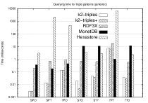
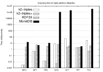
Figure 10: Resolution time (in milliseconds) for triple patterns in jamendo and dbpedia (warm scenario).

The comparison for jamendo includes Hexastore. As can be seen, this is never the best choice and it only outperforms MonetDB in patterns with unbounded predicate. According to these results, we discard it because of its lack competitivity in the current setup. On the contrary, k²-triples⁺ appears as the most efficient choice, and only MonetDB slightly outperforms it for (?,P,?) all collections but dbpedia. Thus, in general, our approach reports the best overall performance for RDF retrieval. This can be analyzed in more detail:

Table 4: Resolution time (in milliseconds) for the patten (?,P,?) on dbpedia (warm scenario)

	k2-triples+	RDF3X	MonetDB
small	0.09	2.53	3.77
big	24.57	14.88	6.14

• Our approach overcomes the main vertical partitioning drawback and provides high performance for resolving patterns with unbounded predicate. This is studied on dbpedia because in these queries scalability is more seriously compromised due to the large number of predicates. k²-triples⁺ leads the scene, whereas RDF3X is close for (S,?,?), falls behind for (?,?,O), and is more than 2 orders of magnitude slower for (S,?,O). As expected, a larger improvement is achieved with respect to our original k²-triples (between 1 and 3 orders of magnitude), whereas our achievement is more significant in comparison with MonetDB: the difference ranges from roughly 5 orders of magnitude in (S,?,?) to 8 orders for (S,?,O).

• MonetDB excels above the other systems in resolving the pattern (?,P,?), but this comparison changes in dbpedia. This owes to the fact that predicates tend to be uniformly used in the other datasets, whereas in dbpedia some predicates are overused and the remaining ones are scarcely used. Thus, the number of results to be obtained differs strongly and it affects the performance. Table 4 summarizes resolution times for predicates returning small and big result sets. As can be seen, k²-triples⁺ dominates for less used predicates, whereas MonetDB is better when more results are retrieved. Thus, the optimized column-oriented representation provides the fastest resolution when the predicate is used in numerous triples, whereas k²-triples⁺ outperforms it for more restictive predicates.

Finally, it is worth noting that k²-triples⁺ obtains a competitive advantage over the original k²-triples for datasets involving many predicates. In the other datasets, this improvement is lower and both techniques achieve comparable performance, yet k²-triples uses sligthly less space as reported above. Nevertheless, we will use k²-triples⁺ in all the remaining experiments.

Joins

After studying triple pattern performance, the next stage in our setup focuses on join resolution. The following experiments (i) analyze how our three different join evaluation algorithms perform: chain, independent and interactive, and (ii) compare them with respect to RDF3X and MonetDB. All these experiments are performed in the warm scenario in order to avoid penalizing on-disk solutions.

Figure 11 summarizes join results for dbpedia. This figure comprises 9 plots, one for each class of join according to the classification described in Figure 8. Each plot comprises three subsets of joins: Subject-Object (SO), Subject-Subject (SS), and Object-Object (OO) in the x axis. The left group considers joins generating a small amount of intermediate results, whereas the right group gives equivalent results for joins involving big intermediate result sets. Resolution times (in milliseconds) are reported on the y axis (logarithmic scale); note that times over $10^{7}$ milliseconds are discarded in all the experiments. We analyze results:

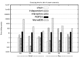
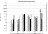
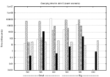
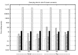
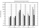
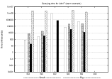
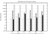
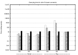
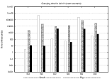
Figure 11: Resolution time (in milliseconds) for joins in dbpedia (warm escenario).

• k²-triples⁺ is the fastest technique for resolving joins in which the value of the two not joined nodes are provided (classes A, D and G). This is mainly because all these classes are resolved using, exclusively, direct and reverse neighbors queries, which are very efficient in practice. Both chain and interactive evaluation algorithms dominate Join A: they report, at least, one order of magnitude of improvement with respect to RDF3X and MonetDB. Chain evaluation is slightly faster in Join D, improving upon RDF3X by more than one order of magnitude (except for OO big). Note that, in this case, MonetDB is no longer competitive since it pays the penalty of resolving a pattern with unbounded predicate. Finally, interactive is the fastest choice for Join G, although chain overcomes it for OO joins. While k²-triples⁺ is always faster than RDF3X in all cases, it is worth noting that differences are reduced due to the need of resolving two patterns with unbounded predicate. Still we remain competitive, while the performance of the vertical partitioning in MonetDB collapses (no times are drawn in this class).

• The second column comprises joins leaving variable a not joined node and fixing the other one (classes B, E, and H). k²-triples⁺ and RDF3X share the lead in these experiments, whereas MonetDB remains competitive only in Join B, although it is never the best choice. On the one hand, the results for Join B and E1 leads to similar conclusions. k²-triples⁺ is the best choice for joins generating small intermediate result sets: chain is fastest for OO, and interactive for SO and SS. RDF3X overcomes k²-triples⁺ when big intermediate result sets are obtained, although our chain evaluation obtains the best perfomance for OO joins. On the other hand, Join E2 and H give similar conclusions, as well. In this case, RDF3X always achieves the best times, except for OO joins, in which chain evaluation is the most efficient choice again. In this case, interactive evaluation is less competitive because it performs multiple range queries.

• The third column comprises joins in which both triple patterns leave as variables their not joined nodes (classes C and F). In Join C, RDF3X is the best choice for SO and OO joins, whereas MonetDB wins for SS. Note that our approach remains competitive for SS and SO, but its performance is significantly degraded for OO. In Join F, our chain evaluation competes with RDF3X for the best times, overcoming it for SS small. However, this arises as the most costly query; note that no technique finishes on OO joins involving big intermediate results.

Summarizing, k²-triples⁺ excels when triple patterns provide values for the non-joined nodes, an it is clearly scalable when predicates are provided as variables. Thus, in general terms, a query optimizer using k²-triples⁺ must favor firstly joins A, D or G; then joins B, E, and H; and finally joins C and F. In any case, joins involving small intermediate result sets are always preferable over those generating big intermediate results.

These findings also apply, in general form, for the remaining datasets in our setup.

8 Conclusions and Future Work

This paper introduces a specific compressed index for RDF called k²-triples. Based on the well-known vertical partitioning model, this technique represents (subject, object) pairs in very sparse binary matrices, which are effectively indexed in compressed space using the novel k²-tree stuctures. This modelling ensures the most compressed representations with respect to a state of the art baseline and also provides the most efficient performance for resolving triple patterns with fixed predicate. To overcome the lack of scalability arising for patterns involving unbounded predicates, two additional indexes are also represented in compressed space. This simple enhancement makes our technique dominant for most RDF retrieval activities. Moreover, we report better numbers for join resolution, outperforming the state of the art for some classes of join, while being competitive in most of the others.

Our future work focuses on getting a full-fledged RDF store over the current k²-triples approach. This means, on the one hand, designing a specific query optimizer able to leverage the current retrieval features and also the reported performance for join operations. This would allow BGPs to be efficiently resolved and set the basis for providing full SPARQL resolution. On the other hand, we will work to obtain a dynamic RDF storage that allows insertion, deletion and updating of triples over the current data partitioning scheme. These objectives are strongly stimulated by the recent advances reported on dynamic k²-trees (?).

- [1]
- [2] [] Abadi, D., Madden, S. and Ferreira, M. (2006), Integrating compression and execution in column-oriented database systems, in ‘Proc. 33th International Conference on Management of Data (SIGMOD)’, pp. 671–682.
- [3]
- [4] [] Abadi, D., Marcus, A., Madden, S. and Hollenbach, K. (2007), Scalable semantic Web data management using vertical partitioning, in ‘Proc. 33th International Conference on Very Large Data Bases (VLDB)’, pp. 411–422.
- [5]
- [6] [] Abadi, D., Marcus, A., Madden, S. and Hollenbach, K. (2009), ‘SW-store: a vertically partitioned DBMS for semantic Web data management’, The VLDB Journal 18, 385–406.
- [7]
- [8] [] Angles, R. and Gutiérrez, C. (2005), Querying RDF data from a graph database perspective, in ‘Proc. 2nd European Semantic Web Conference (ESWC)’, pp. 346–360.
- [9]
- [10] [] Arias, M., Fernández, J. and Martínez-Prieto, M. (2011), An empirical study of real-world SPARQL queries, in ‘Proc. 1st International Workshop on Usage Analysis and the Web of Data (USEWOD)’. Available at http://arxiv.org/abs/1103.5043.
- [11]
- [12] [] Atre, M., Chaoji, V., Zaki, M. and Hendler, J. (2010), Matrix “bit” loaded: a scalable lightweight join query processor for RDF data, in ‘Proc. 19th International Conference on World Wide Web (WWW)’, pp. 41–50.
- [13]
- [14] [] Auer, S., Bizer, C., Kobilarov, G., Lehmann, J., Cyganiak, R. and Ives, Z. (2007), DBpedia: a nucleus for a Web of open data, in ‘Proc. 6th International Semantic Web (ISWC) Conference and 2nd Asian Semantic Web Conference (ASWC)’, pp. 722–735.
- [15]
- [16] [] Berners-Lee, T., Hendler, J. and Lassila, O. (2001), ‘The semantic Web’, Scientific American Magazine .
- [17]
- [18] [] Binna, R., Gassler, W., Zangerle, E., Pacher, D. and Specht, G. (2011), SpiderStore: A native main memory approach for graph storage, in ‘Proc. 23rd Workshop Grundlagen von Datenbanken (GvDB)’, pp. 91–96.
- [19]
- [20] [] Bizer, C., Heath, T. and Berners-Lee, T. (2009), ‘Linked data – the story so far’, International Journal on Semantic Web and Information Systems 5, 1–22.
- [21]
- [22] [] Bönström, V., Hinze, A. and Schweppe, H. (2003), Storing RDF as a graph, in ‘Proc. 1st Latin American Web Congress (LA-WEB)’, pp. 27–36.
- [23]
- [24] [] Brisaboa, N., de Bernardo, G. and Navarro, G. (2012), Compressed dynamic binary relations, in ‘Proc. 22th Data Compression Conference (DCC)’, pp. 52–61.
- [25]
- [26] [] Brisaboa, N., Ladra, S. and Navarro, G. (2009a), Directly addressable variable-length codes, in ‘Proc. 16th International Symposium on String Processing and Information Retrieval (SPIRE)’, pp. 122–130.
- [27]
- [28] [] Brisaboa, N., Ladra, S. and Navarro, G. (2009b), K2-trees for compact Web graph representation, in ‘Proc. 16th International Symposium on String Processing and Information Retrieval (SPIRE)’, pp. 18–30.
- [29]
- [30] [] Broekstra, J., Kampman, A. and van Harmelen, F. (2003), Spinning the Semantic Web, MIT Press, chapter Sesame: An architecture for storing and querying RDF data and schema information, pp. 197–222.
- [31]
- [32] [] Claude, F. and Ladra, S. (2011), Practical representations for Web and social graphs, in ‘Proc. 20th ACM Conference on Information and Knowledge Management (CIKM)’, pp. 1185–1190.
- [33]
- [34] [] Fernández, J. D., Martínez-Prieto, M. A., Gutiérrez, C. and Polleres, A. (2011), Binary RDF Representation for Publication and Exchange (HDT), W3C Member Submission. http://www.w3.org/Submission/2011/03/.
- [35]
- [36] [] Fernández, J. D., Martínez-Prieto, M. A., Gutiérrez, C., Polleres, A. and Arias, M. (2013), ‘Binary RDF Representation for Publication and Exchange (HDT)’, Journal of Web Semantics . In Press. Available at: http://dx.doi.org/10.1016/j.websem.2013.01.002.
- [37]
- [38] [] González, R., Grabowski, S., Mäkinen, V. and Navarro, G. (2005), Practical implementation of rank and select queries, in ‘Proc. Posters of 4th Workshop on Experimental Algorithms (WEA)’, pp. 27–38.
- [39]
- [40] [] Groppe, S. (2011), Data Management and Query Processing in Semantic Web Databases, Springer.
- [41]
- [42] [] Groza, T., Grimnes, G., Handschuh, S. and Decker, S. (2013), ‘From raw publications to linked data’, Knowledge and Information Systems 34, 1–21.
- [43]
- [44] [] Harris, S. and Gibbins, N. (2003), 3store: Efficient bulk RDF storage, in ‘Proc. 1st International Workshop on Practical and Scalable Semantic Systems (PSSS)’, pp. 1–15.
- [45]
- [46] [] Harth, A. and Decker, S. (2005), Optimized index structures for querying RDF from the Web, in ‘Proc. 3rd Latin American Web Congress (LA-WEB)’, pp. 71–80.
- [47]
- [48] [] Hayes, J. and Gutiérrez, C. (2004), Bipartite graphs as intermediate model for RDF, in ‘Proc. 3rd International Semantic Web Conference (ISWC)’, pp. 47–61.
- [49]
- [50] [] Huang, J., Abadi, D. and Ren, K. (2011), ‘Scalable SPARQL querying of large RDF graphs’, Proceedings of the VLDB Endowment 4(11), 1123–1134.
- [51]
- [52] [] Janik, M. and Kochut, K. (2005), BRAHMS: A workbench RDF store and high performance memory system for semantic association discovery, in ‘Proc. 4th International Semantic Web Conference (ISWC)’, pp. 431–445.
- [53]
- [54] [] Jing, Y., Jeong, D. and Baik, D. (2009), ‘Sparql graph pattern rewriting for owl-dl inference queries’, Knowledge and Information Systems 20, 243–262.
- [55]
- [56] [] Knuth, D. (1973), The Art of Computer Programming, volume 3: Sorting and Searching, Addison Wesley.
- [57]
- [58] [] Ladra, S. (2011), Algorithms and Compressed Data Structures for Information Retrieval, PhD thesis, Department of Computer Science, University of A Coruña, Spain.
- [59]
- [60] [] Manola, F. and Miller, E., eds (2004), RDF Primer, W3C Recommendation. http://www.w3.org/TR/rdf-primer/.
- [61]
- [62] [] Martínez-Prieto, M., Fernández, J. and Cánovas, R. (2012), ‘Querying RDF dictionaries in compressed space’, ACM SIGAPP Applied Computing Reviews 12(2), 64–77.
- [63]
- [64] [] Navarro, G. and Mäkinen, V. (2007), ‘Compressed full-text indexes’, ACM Computing Surveys 39(1), article 2.
- [65]
- [66] [] Neumann, T. and Weikum, G. (2009), Scalable join processing on very large RDF graphs, in ‘Proc. 35th International Conference on Management of Data (SIGMOD)’, pp. 627–640.
- [67]
- [68] [] Neumann, T. and Weikum, G. (2010), ‘The RDF-3X engine for scalable management of RDF data’, The VLDB Journal 19, 91–113.
- [69]
- [70] [] Prud’hommeaux, E. and Seaborne, A., eds (2008), SPARQL Query Language for RDF, W3C Recommendation. http://www.w3.org/TR/rdf-sparql-query/.
- [71]
- [72] [] Ramakrishnan, R. and Gehrke, J. (2000), Database Management Systems, Osborne/McGraw-Hill.
- [73]
- [74] [] Sakr, S. and Al-Naymat, G. (2010), ‘Relational processing of RDF queries: a survey’, SIGMOD Records 38, 23–28.
- [75]
- [76] [] Sakr, S., Elnikety, S. and He, Y. (2012), G-SPARQL: a hybrid engine for querying large attributed graphs, in ‘Proc. 21st ACM Conference on Information and Knowledge Management (CIKM)’, pp. 335–344.
- [77]
- [78] [] Salomon, D. (2007), Variable-length Codes for Data Compression, Springer.
- [79]
- [80] [] Samet, H. (2006), Foundations of Multidimensional and Metric Data Structures, Morgan Kaufmann Publishers Inc.
- [81]
- [82] [] Sánchez, D., Isern, D. and Millan, M. (2011), ‘From raw publications to linked data’, Knowledge and Information Systems 27, 393–418.
- [83]
- [84] [] Schmidt, M., Hornung, T., Küchlin, N., Lausen, G. and Pinkel, C. (2008), An experimental comparison of RDF data management approaches in a SPARQL benchmark scenario, in ‘Proc. 7th International Conference on The Semantic Web (ISWC)’, pp. 82–97.
- [85]
- [86] [] Sidirourgos, L., Goncalves, R., Kersten, M., Nes, N. and Manegold, S. (2008), ‘Column-store support for RDF data management: not all swans are white’, Proceedings of the VLDB Endowment 1(2), 1553–1563.
- [87]
- [88] [] Stonebraker, M., Abadi, D., Batkin, A., Chen, X., Cherniack, M., Ferreira, M., Lau, E., Lin, A., Madden, S., O’Neil, E., O’Neil, P., Rasin, A., Tran, N. and Zdonik, S. (2005), C-store: a column-oriented DBMS, in ‘Proc. 31st International Conference on Very Large Data Bases (VLDB)’, pp. 553–564.
- [89]
- [90] [] Urbani, J., Maassen, J. and Bal, H. (2010), Massive semantic Web data compression with MapReduce, in ‘Proc. 19th ACM International Symposium on High Performance Distributed Computing (HPDC)’, pp. 795–802.
- [91]
- [92] [] Weiss, C., Karras, P. and Bernstein, A. (2008), ‘Hexastore: Sextuple indexing for semantic Web data management’, Proceedings of the VLDB Endowment 1(1), 1008–1019.
- [93]
- [94] [] Wilkinson, K. (2006), Jena property table implementation, in ‘Proc. 2nd International Workshop on Scalable Semantic Web Knowledge Base Systems (SSWS)’, pp. 35–46.
- [95]