Numerical and Experimental Study of the Interaction between two Marine Current Turbines

Abstract

The understanding of interaction effects between marine energy converters represents the next step in the research process that should eventually lead to the deployment of such devices. Although some a priori considerations have been suggested recently, very few real condition studies have been carried out concerning this issue.

Trials were run on 1/30^th scale models of three-bladed marine current turbine prototypes in a flume tank. The present work focuses on the case where a turbine is placed at different locations in the wake of a first one. The interaction effects in terms of performance and wake of the second turbine are examined and compared to the results obtained on the case of one single turbine. Besides, a three-dimensional software, based on a vortex method is currently being developed, and will be used in the near future to model more complex layouts.

The experimental study shows that the second turbine is deeply affected by the presence of an upstream device and that a compromise between individual device performance and inter-device spacing is necessary. Numerical results show good agreement with the experiment and are promising for the future modelling of turbine farms.

Abstract

The understanding of interaction effects between marine energy converters represents the next step in the research process that should eventually lead to the deployment of such devices. Although some a priori considerations have been suggested recently, very few real condition studies have been carried out concerning this issue.

Trials were run on 1/30^th scale models of three-bladed marine current turbine prototypes in a flume tank. The present work focuses on the case where a turbine is placed at different locations in the wake of a first one. The interaction effects in terms of performance and wake of the second turbine are examined and compared to the results obtained on the case of one single turbine. Besides, a three-dimensional software, based on a vortex method is currently being developed, and will be used in the near future to model more complex layouts.

The experimental study shows that the second turbine is deeply affected by the presence of an upstream device and that a compromise between individual device performance and inter-device spacing is necessary. Numerical results show good agreement with the experiment and are promising for the future modelling of turbine farms.

1 Introduction

A new level has been recently reached in the deployment of marine energy converters with the launching of several large-scale projects. For instance, India plans to install a 250MW tidal farm on its west coast, with a first implantation of fifty AK1000 (Atlantis Resources) turbines of 1MW each [1]. In 2011, the Scottish Government announced its approval for a 10MW tidal power array project on Scotland’s west coast. It would consist of ten HS1000 (Hammerfest Strøm) turbines that should be installed from 2013 to 2015 [2]. Marine Current Turbines Ltd also announced in March 2011 that it had submitted a consent application to install in 2015 a 10MW tidal farm off the Anglesey coast, in Wales [3]. Some a priori studies have already been carried out to evaluate the potential retrievable power in specific areas, for instance the Race of Alderney, off the Cap de la Hague in France [4].

The behaviour of single marine energy converters such as marine current turbines is now globally well understood thanks to experimental and numerical studies [5, 6, 7]. However, as the size of such arrays is expected to grow with time, the issue of interaction effects between turbines, most importantly negative ones, has to be addressed. Some a priori considerations and suggestions have been presented in recent studies [8, 9] about different parameters of a marine current turbines array layout. As regards interaction effects, numerical studies on vertical axis tidal turbines have been carried out, such as [10] about the torque fluctuation.

The aim of the present paper is to give an idea of the interaction characteristics between two horizontal axis current turbines in real condition configurations. It complements a previous experimental study [7] carried on different but similar blade geometries and additional rotation speeds. Another purpose is to validate the three-dimensional software on a single device configuration, before extending it to multi-devices cases in the future. The main point is to be able to model more complex turbines array layouts, which cannot be set up in flume tanks.

The first part of this paper is thus dedicated to the characterisation of a single marine current turbine behaviour and to the validation of the numerical software on these cases. The second part presents experimental trials on two-device configurations and uses the results on single device configurations as a comparison. Conclusions can then be drawn on the interaction effects between two marine current turbines. A comparison with the latest numerical results is also briefly presented. Eventually, conclusions are drawn and an outlook on both numerical and experimental future work is given.

2 Single-device configuration

Trials have been performed at the French Research Institute for Exploitation of the Sea (IFREMER) on a 1/30^th scale model of a three-bladed turbine prototype, in a 18$\times{}$4$\times{}$2m wave and current flume tank. The prototype consists of a rotor, which is $0.7$m in diameter, and a $0.7$m long axial hub (cf. figure 1). The blockage ratio is then less than 5%. The turbine blades are designed from a NACA63418 profile.

Force and moment on the turbine are measured thanks to six-component load cells, while velocity measurements are obtained thanks to a two component Laser Doppler Velocimetry (LDV) system. The experimental setup is presented in details in [7]. In this section, experimental trials, concerning the wake behind the turbine and the performance of the device, are presented. Corresponding numerical results are shown in order to validate the numerical tool.

2.1 Description of the parameters

A marine current turbine may be subject to various parameters that can influence its behaviour, amongst others:

• The current velocity $\mathbf{U}_{\infty}$ which is assumed to be uniform and such that

  $$\mathbf{U}_{\infty}=U_{\infty}\mathbf{e}_{x}$$ (1)

• The Tip Speed Ratio (TSR):

  $$TSR=\frac{\Phi R}{U_{\infty}}$$ (2)

  where $R=D/2$ denotes the rotor radius and $\Phi$ the rotation speed of the turbine.

• The ambient turbulence intensity rate (TI) defined by

  $$TI=100\frac{\sqrt{\frac{1}{3}(\sigma_{u}^{2}+\sigma_{v}^{2}+\sigma_{w}^{2})}}{\sqrt{\bar{u}^{2}+\bar{v}^{2}+\bar{w}^{2}}}$$ (3)

  where $u$, $v$ and $w$ are respectively the $x$, $y$ and $z$ velocity components, $\bar{q}$ denotes the mean value and $\sigma_{q}$ the standard deviation of quantity $q$.

These parameters, as well as the flume tank and turbine geometries are summarized on figure 1.

Figure 1: Description of the single configuration parameters. The origin $O(0;0;0)$ is chosen at the rotor centre.

In the present study, an incoming velocity of 0.8m/s is considered, as well as TSR values between 0 and 10, and ambient TI of 3% and 15%. The turbulence in the flow is induced by the current generator of the flume tank. Without the use of a honeycomb, a turbulence intensity rate of 15% is measured, which can be reduced to 3% by placing honeycomb grids at the beginning of the flume. LDV Measurements, performed at different locations in the area swept by the turbine blades, indicate that these sources of turbulence imply an homogeneous turbulence structure.

2.2 Characterization of the wake

The general aspect of the wake behind a marine current turbine can be estimated by drawing velocity and turbulence maps of the downstream flow. Such maps can provide useful information to characterize the impact of the turbine on its close environment.

The LDV measurements are performed on a grid whose nodes $(X_{i},Y_{i})$ are arranged as follows:

• $X_{1}=1.2D$ and $X_{i}=i\times D$ for $i=2,\ldots,10$.

• $Y_{i}=-1.2+(i-1)\times 0.1$m for $i=1,\ldots,25$, with two additional positions $Y_{26}=-Y_{27}=R=0.35$m;

The measurement on each node lasts 100 seconds with an observed data rate between 7 and 17Hz.

The downstream turbulence $TI_{down}$ is evaluated as a turbulence intensity rate in the $xOy$ plan:

$$TI_{down}=100\frac{\sqrt{\frac{1}{2}(\sigma_{u}^{2}+\sigma_{v}^{2})}}{\sqrt{\bar{u}^{2}+\bar{v}^{2}}}$$ (4)

As for the axial velocity, $u/U_{\infty}$ is considered, which represents the proportion of velocity recovered behind the turbine in comparison to the upstream velocity $U_{\infty}$.

Figure 2 shows axial velocity and turbulence maps for different upstream ambient TI with a turbine at TSR=3.67. These maps point out that a higher ambient TI rate reduces the wake length in terms of velocity and turbulence. Indeed, figure 2(b) shows that at a distance of seven diameters behind the turbine in a 15% ambient TI, the axial velocity profile tends to recover its uniformity and about 90% of its intensity. On the other hand, the profile at the same location for an ambient 3% TI (figure 2(a)) remains very wake-shape like, with only 65% of $U_{\infty}$ recovered at the centre. Even 10 diameters behind the turbine, the profile is still non-uniform and below the oncoming velocity, with about 75% recovered at the centre. The same behaviour can be observed with the downstream turbulence. Indeed, with a 3% ambient TI, figure 2(c) shows that $10$ diameters behind the turbine, the downstream TI remains higher than 3%. On the contrary, it goes back to 15% in the case of an upstream 15% TI (figure 2(d)).

These experiments have been performed in the same conditions as in [7] but with a lower TSR to be able to compared them with numerical computations [11]. As a matter of fact, as stated in section 2.3, computations with too high TSR are not valid because of the particles emission model. Another significant difference resides in the use of new blades that are not patented, with a shorter chord, so as to avoid confidentiality restrictions.

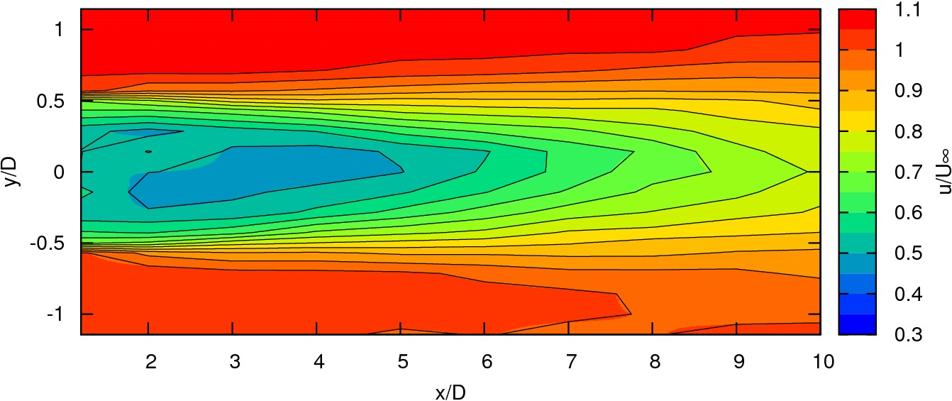
(a) Axial velocity map (TI=3%)

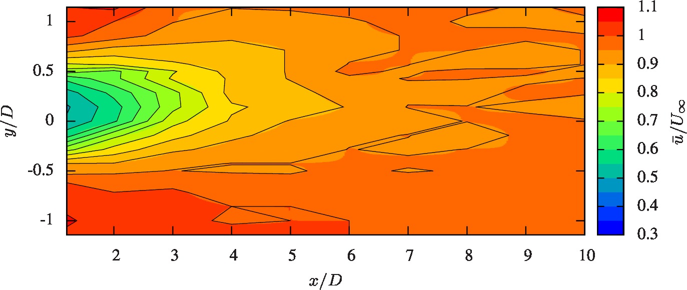
(b) Axial velocity map (TI=15%)

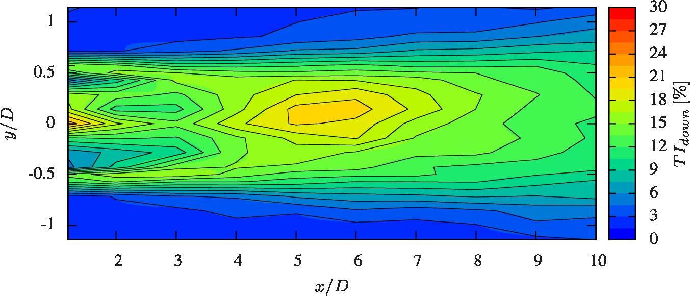
(c) Turbulence map (TI=3%)

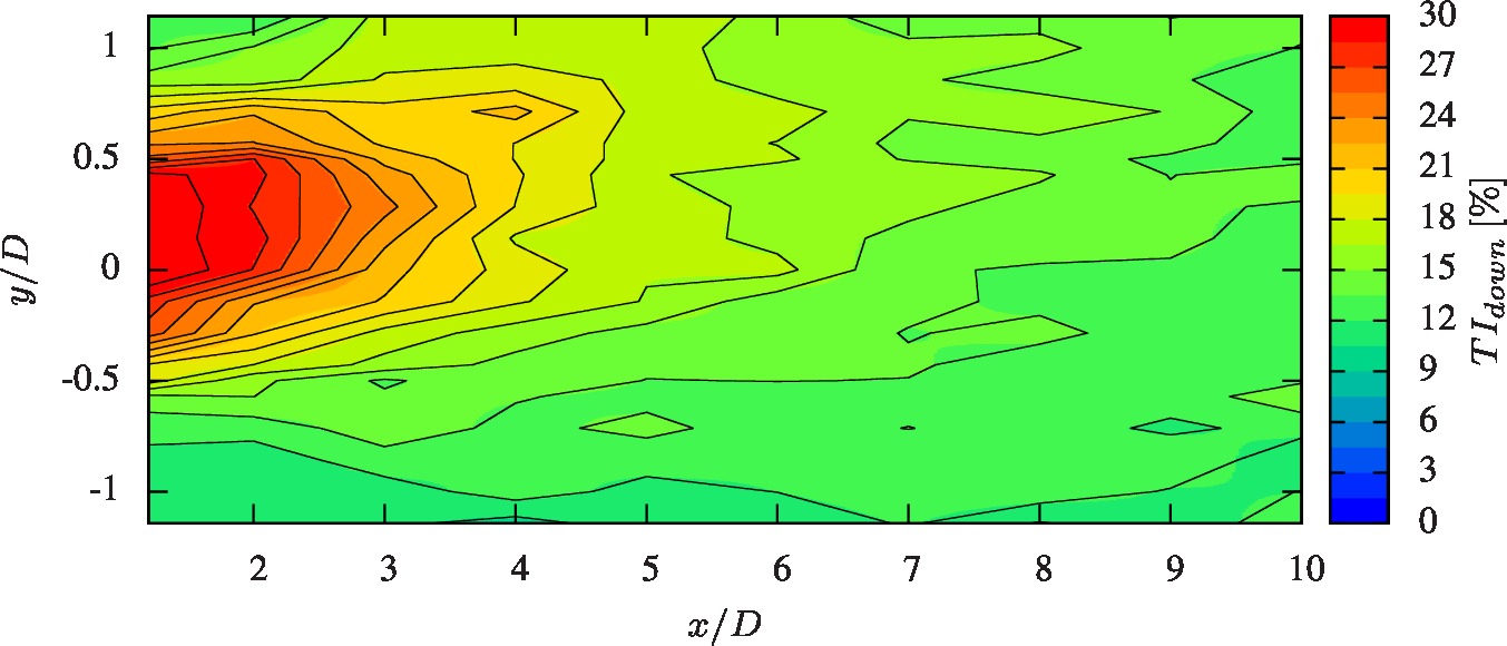
(d) Turbulence map (TI=15%)

Figure 2: Wake behind a turbine with TSR=3.67

2.3 Comparison with numerical results

A three-dimensional software is under development in the LOMC laboratory of Le Havre University, based on a Lagrangian vortex particle method [12, 13, 14, 15, 16]. The vortical flow is discretized into particles, which are small volumes of fluid carrying intrinsic physical quantities such as their position and vorticity. Those particles are emitted at the trailing edge of the obstacle according to the Kutta-Joukowski condition and then advected in a Lagrangian frame thanks to the Navier-Stokes equations for an incompressible flow. The details of the method are presented in [17, 11].

Velocity maps can also be drawn from the numerical computations. Figure 3 presents an axial velocity map obtained from a numerical computation and shows that the general aspect of the wake is well reproduced. It should be pointed out that all of the computations are performed with a 0% ambient TI, with a Large Eddy Simulation (LES) turbulence model.

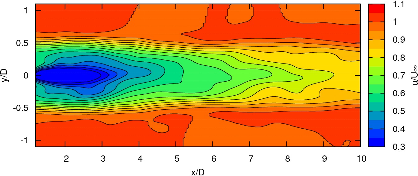
Figure 3: Axial velocity map from computation with TSR=3.67, TI=0% and a turbulence model.

A closer look can be taken by considering a velocity profile at one particular distance behind the turbine. Figure 4 shows both experimental and numerical profiles 1.2 diameter behind the turbine. From these profiles one can also estimate the mean value of the axial velocity $\bar{u}(x)$ at position $x$ integrated on a $R^{*}=R+\delta r$ radius disc:

$$\bar{u}(x)=\frac{1}{{R^{*}}^{2}}\int_{-R^{*}}^{R^{*}}|y|u(x,y)\,\mathrm{d}y$$ (5)

Here $\delta r=0.05\mathrm{m}\simeq 0.14R$ is considered, which enlarges the integration interval to the two nearest experimental measurement nodes outside the rotor. In that manner, the whole velocity deficit is accounted for. The $R^{*}$ radius disc thus represents the turbine’s area of influence, which is slightly larger than the turbine’s cross-section area. The numerical profile fits quite well with the experiment, even though the mean value seems to be slightly underestimated and the shape of the deficit is not accurately represented at the centre. This can be explained by the numerical turbulence model, which is not sophisticated enough at the present time and will be improved in the near future.

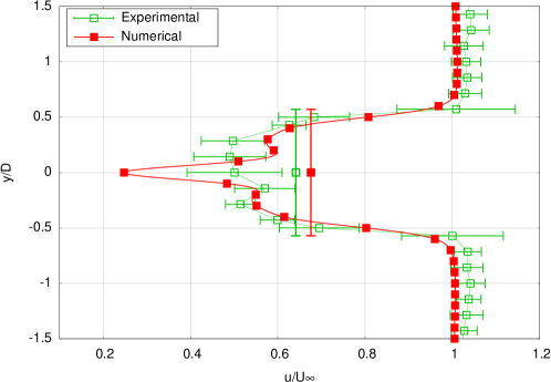
Figure 4: Numerical (TI=0% with turbulence model) and experimental (TI=3%) axial velocity profile with TSR=3.67. Horizontal bars on the experimental curve represents the standard deviation and vertical bars represent the mean value of the axial velocity integrated on a $R+\delta r$ radius disc. The tips of the vertical bars represent the integration diameter for the estimation of the mean values (i.e. $2(R+\delta r)$).

Now that the evaluation of the axial velocity mean value on the turbine’s area of influence has been defined, one can examine the reduction of the velocity deficit as the distance from the turbine increases. The mean axial velocity deficit $\gamma$ (in %) at a specific location $x$ behind the turbine is defined as:

$$\gamma(x)=100(1-\bar{u}(x))$$ (6)

This definition leads to figure 5, on which one can see that with an ambient 3% TI, the experimental velocity deficit steadily decreases from about 35% at $x<2D$ down to 15% at $x=10D$. On the other hand, with a 15% TI, the deficit decreases sharply in the near wake and then levels off around 8% from $x=5D$. The relation between the velocity deficit (and therefore the velocity as well) and the distance from the turbine seems to be linear in the case of an ambient 3% TI. An equivalent numerical curve corresponding to the wake presented in figure 3 is also shown in order to check that the wake dynamics is numerically well reproduced. A better turbulence model should enable us to compute more accurately and to distinguish the 3% and 15% TI configurations.

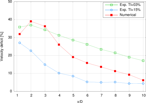
Figure 5: Mean velocity deficit behind the turbine for varying TI as values of 3% and 15% in the experiment, and a TI of 0% together with a turbulence model in the computation.

Another aspect of the behaviour of a marine current turbine can be deduced from the forces and moments on the turbine blades. More particularly, the axial moment or torque is used to determine the turbine power coefficient $C_{P}$ that assesses its performance. Besides, the axial force can provide information about the fatigue of the machine and is used for the calculation of the thrust coefficient $C_{T}$.

The power coefficient is defined as the proportion of power $\mathcal{P}$ retrieved by the turbine as compared to the maximum power available from the incoming flow through the rotor area:

$$C_{P}=\frac{\mathcal{P}}{\frac{1}{2}\rho SU_{\infty}^{3}}=\frac{\mathcal{M}_{x}\Phi}{\frac{1}{2}\rho\pi R^{2}U_{\infty}^{3}}=\frac{\mathcal{M}_{x}}{\frac{1}{2}\rho\pi R^{3}U_{\infty}^{2}}\times TSR$$ (7)

where $\rho$ is the density of the fluid, $S$ is the cross-section area of the turbine and $\mathcal{M}_{x}$ is the axial moment, also referred to as the turbine torque, defined as the $x$-component of the moment. Similarly, the thrust coefficient is defined as the axial force $T$ acting upon the turbine as compared to the kinetic energy of the incoming flow through $S$:

$$C_{T}=\frac{T}{\frac{1}{2}\rho\pi R^{2}U_{\infty}^{2}}=\frac{T}{\frac{1}{2}\rho\pi R^{3}U_{\infty}\Phi}\times TSR$$ (8)

For a given current velocity of 0.8m/s, and an ambient TI of 3%, figure 6 presents the evolution of power and thrust coefficients of a turbine function of its TSR. Figure 6(a) shows that approximately 40% of the total available power is retrieved by the turbine ($C_{P}\simeq 0.4$) when its TSR is between three and four. Once again, these curves are compared to results obtained from numerical computations, which show very good agreement. However, the numerical particle emission model does not account for flow separation, which explains why for TSR higher than three, the $C_{P}$ keeps increasing in the numerical computations while it should reach a peak and then decrease. The modelling of flow separation with a vortex method is currently being considered and should be implemented soon.

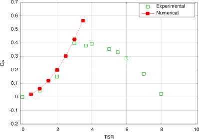
(a) $C_{P}$ function of TSR

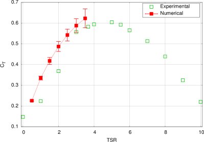
(b) $C_{T}$ function of TSR

Figure 6: Evaluation of Power ($C_{P}$) and Thrust ($C_{T}$) coefficients, with a 3% ambient TI in the experiment. The corresponding evolution for the computations has been obtained with a TI of 0% with a turbulence model. The numerical points represent the mean values computed over $\Delta t=2$s and the vertical bars represent the standard deviation with respect to this mean value.

Other configurations and blades have been tested to validate the software in terms of $C_{P}$ and $C_{T}$, in particular from [18], to examine the influence of the blades set angle and to check the convergence of the method [11]. As pointed out, development is still necessary to improve the accuracy of computations. More particularly, the turbulence model needs to be more sophisticated, which is why one of the first priority is to find an adequate model amongst those presented in [19], for instance. In order to assess correctly a turbine performance, the emission model of the numerical method also needs to be altered so as to account for flow separation. Once those modifications are achieved, focus will be made on the modelling of multi-device configurations and corresponding validation will be possible thanks to the experimental results presented in the next section of this paper. The main interest of the fully-validated software will be to model with accuracy more complex layouts that cannot be set up in experimental trial facilities.

3 Marine current turbines interaction

3.1 General considerations

Studies concerning the layout of marine current turbines arrays are still few. However, general guidelines and a priori considerations can be found in recent literature [8, 9]. Two kinds of arrays have to be distinguished, first generation and second generation arrays, so called because of the probable progressive row by row growth of these farms. First generation arrays designate the youngest farms, made up of a single or two rows, designed to avoid any interaction effect between the turbines. On the contrary, second generation arrays refer to larger arrays in which such interactions cannot be avoided [8].

It is then clear that those two designations have a chronological meaning. As a matter of fact, at an early age of their implantation, arrays will be made up of one or two rows of turbines, the second row being placed downstream the first one and shifted so that the wakes of the upstream devices will not interact with the turbines of the second row. The early extensions of such arrays will be performed by adding new devices into the one or two existing rows, but a time will come when the only way to enlarge first generation arrays will consist in adding rows. From then on, interactions between turbines will no longer be avoidable. Figure 7 illustrates such a layout.

Figure 7: Schematic top view of a marine current turbines array.

Several parameters, besides the depth of the array in the flow that is considered here to be far enough from both the free surface and the sea bed in order to neglect their interaction, are characteristic of an array layout:

• The distance $a_{1}$ between two successive “even” rows;

• The distance $a_{2}$ between two successive “odd” rows;

• The distance $a_{3}$ between an upstream even row and the very next (odd) row;

• The distance $b_{1}$ between two adjacent turbines of a same row;

• The $y$-offset $b_{2}$ between two successive current perpendicular lines of turbines.

Some suggestions can be made concerning those parameters. In particular, it would be natural to consider that $b_{2}=\frac{1}{2}b_{1}$, as it has been suggested in [8]. Similarly, parameters $a_{1}$, $a_{2}$ and $a_{3}$ can be chosen such that $a_{1}=a_{2}=2a_{3}$. However, the choice of a smaller $a_{3}$ would also make sense so as to benefit from potential “positive” interactions from the upstream turbines.

The present study focuses on the layout of second generation arrays issue, and more particularly on the characterization of the interaction effects between two marine current turbines placed one behind another. Hence parameter $a_{1}$ alone describes the configuration, and will then simply be referred to as $a$.

3.2 Experimental setup

The experimental setup is made up of two 1/30^th scale turbine models attached to one (for $a\leq 5D$ configurations) or two (for $a>5D$ configurations) lengthwise girder(s) thanks to two poles of the same length. A photography of the setup with $a=4D$ is given in figure 8.

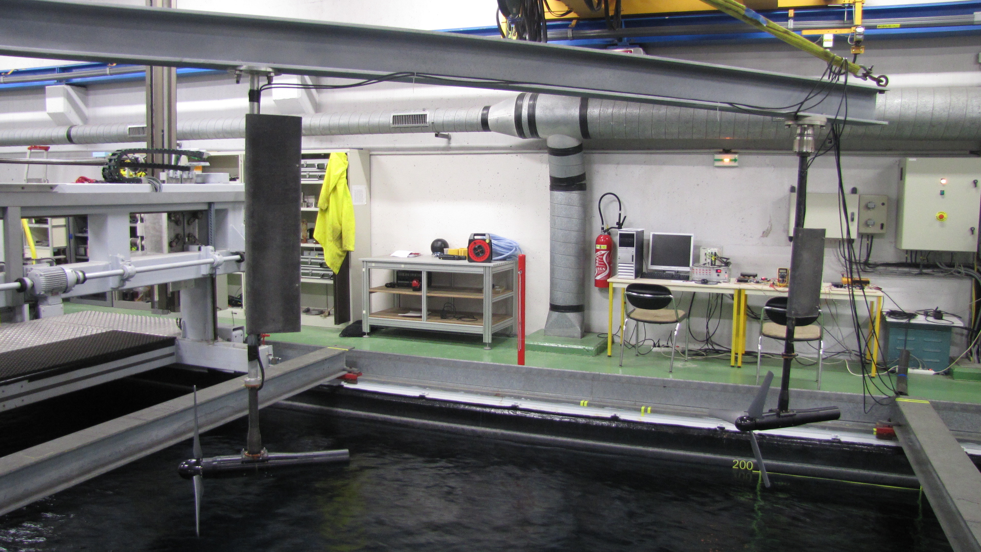
Figure 8: Photography of the experimental setup with $a=4D$. For $a>5D$ configurations, the lengthwise girder is split into two smaller girders and two additional transerse girders are used to support them (cf. figure 9).

The girder is placed over the flume tank, parallel to the upstream current and at equal distance from the two sides. The downstream turbine is equipped with a six-component load cell and a two-component laser is attached to a footbridge over the flume. The laser can move along the footbridge that can itself be shifted backward and forward along the flume. The Laser Doppler Velocimetry (LDV) technique is used to measure axial and radial velocities at different locations on a grid behind the downstream turbine. This allows to draw maps such as those of figure 2 shown in section 2.2. Schematic views of the complete setup are given in figure 9.

(a) Side view

(b) Top view

Figure 9: Schematic view of the experimental setup for configurations with $a>5D$. The origin $O(0;0;0)$ is chosen at the center of the downstream turbine rotor.

3.3 Wake interactions

This study of wake interactions focuses on a $a=4D$ configuration, with both TSR=3.67 and an upstream 3% ambient TI. This is motivated by the results obtained with a single turbine (cf. section 2.2). As a matter of fact, when looking at figure 2(c), one can see that the turbulence intensity rate four diameters behind the turbine is in the order of 15%. It should thus be relevant to compare this case to the single device configuration in a 15% ambient TI due to the current generation process in the flume tank without any “smoothing” techniques (e.g. using a honeycomb to reduce the ambient TI; for more detail, see [7]). If the downstream device in the $a=4D$ configuration behaves as if it were single, this would mean that there is no wake interactions per se and that the ambient TI rate represents the only affecting “input” parameters for the behaviour of interacting turbines.

In the single device configuration, figures 2(b) and 5 show that the velocity deficit behind a turbine in a 15% turbulent upstream flow tends to reduce rapidly. This represents a significant advantage with a view to place a second turbine in the wake of the first one. On the other hand, in the case of interacting turbines, axial velocity and turbulence maps behind the downstream turbine are drawn in figure 10 . Since the downstream turbine is placed in an area where the mean turbulence intensity rate is close to 15%, the general aspect of its wake may look like the wake of a single turbine in a 15% ambient TI. Unfortunately, one can easily see that this is not the case, which indicates that there is a real interaction between the two turbines.

This suggests that the turbulence induced by the current generation process and the one induced by the turbine do not present the same characteristics. A complementary study was recently carried out with two turbines in a 15% upstream ambient TI in order to determine whether the presence of the upstream turbine modifies the turbulence structure [20].

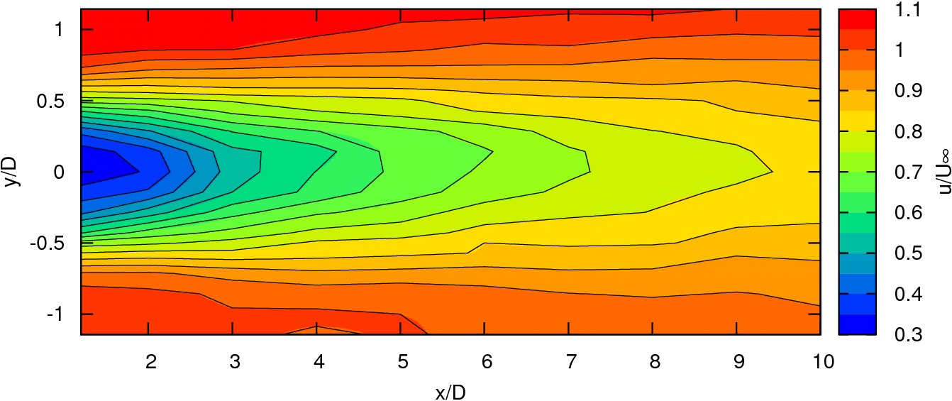
(a) Axial velocity map

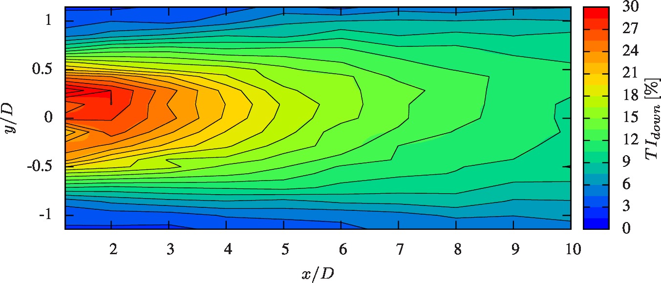
(b) Turbulence map

Figure 10: Wake behind the second turbine with $a=4D$, upstream TI=3% and both TSR=3.67.

3.4 Downstream performance

Another way to evaluate the interaction effects between two turbines is to examine the performance of the downstream turbine. The comparison with the performance of a single device gives an idea on how deeply a turbine is affected by the presence of an upstream device. The evolution of the downstream turbine $C_{P}^{down}$ is plotted against its TSR on figure 11(a), for different $a/D$ configurations, and with an upstream device TSR of three, which yields maximum individual energy. The evolution of the single device $C_{P}^{single}$ function of its TSR, already shown in section 2.3, is also plotted as a matter of comparison. It should be noted that the TSR of the downstream turbine is computed thanks to equation (2) where $U_{\infty}$ is the upstream velocity before the first device, and thus not the mean velocity at the location of the second device. This choice is motivated by the fact that in real conditions, one will not be able to access the actual velocity at the location of the downstream turbine. The present study of interaction effects between turbines is thus carried out considering only “measurable” upstream quantities. By doing so, general conclusions may be drawn about the behaviour of interacting turbines depending only on those input parameters. Similarly, the downstream turbine $C_{P}^{down}$ is still computed from the upstream velocity $U_{\infty}$. It is then important to understand that $C_{P}^{down}$ is an abuse of notation since this quantity does not represent any power coefficient; it can only be an indicator of the power retrieved as compared to the upstream velocity $U_{\infty}$.

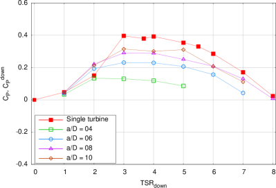
(a) $C_{P}^{down}$ of the downstream device function of its TSR, with an upstream TSR of 3 and an ambient TI of 3%, compared to the $C_{P}^{single}$ of a single turbine shown in section 2.3.

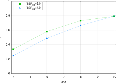
(b) Maximum $C_{P}^{down}$ obtained on the downstream turbine function of the inter-device distance, for two different upstream TSR.

Figure 11: Performance evaluation of the twin-device configuration.

The experiment shows that the maximum $C_{P}^{down}$ for the downstream turbine is obtained with a downstream turbine TSR between three and four, except for the $a=4D$ configuration where the $C_{P}^{down}$ is slightly better with TSR=2. One can also notice that the longer the distance between the two devices is, the better the evolution of the downstream turbine $C_{p}^{down}$ fits with a single turbine $C_{P}^{single}$. This is clearly due to the fact that the velocity deficit generated by a turbine decreases as a function of the distance from the device (cf. figure 5).

This trend can be confirmed by plotting the value of the maximum $C_{P}^{down}$ obtained for each $a/D$ configuration. The “efficiency” $\eta$ is defined as the ratio of the maximum $C_{P}^{down}$ of the downstream device to the maximum $C_{P}^{up}$ of the upstream device, that is to say the one obtained with TSR=3 for a single device:

$$\eta=\frac{\max\big{(}C_{P}^{down}(TSR)\big{)}}{\max\big{(}C_{P}^{up}(TSR)\big{)}}=\frac{\max\big{(}C_{P}^{down}(TSR)\big{)}}{C_{P}^{single}(TSR=3)}$$ (9)

Figure 11(b) shows the evolution of $\eta$ function of the distance $a/D$, for upstream device TSR of 3 and 4. As expected, the maximum $C_{P}^{down}$ raises as $a$ increases and reaches 80% of the maximum retrievable power for a single device when $a/D=10$. It should be pointed out that the downstream device can retrieve more power when the upstream turbine has its TSR=3 rather than 4. These results indicate that a compromise between individual performance and inter-device spacing is necessary. Considering an implantation area of given shape and surface, the more distant two successive rows of turbines, the higher the individual power retrieved; but there is then less space for additional rows of devices, that is to say that fewer turbines can be implanted. Hence a complete compromise has to be made considering the implantation of marine current turbines farms.

3.5 Comparison with numerical results

Coarse numerical simulations were run with two turbines with $a=4D$, and $TSR=TSR^{up}=TSR^{down}=3.67$. Since there is no maximum in the numerical $C_{P}$ curves, the ratio $r_{C_{P}}$ for two turbines with the same TSR is defined as follows:

$$r_{C_{P}}(TSR)=\frac{C_{P}^{down}(TSR)}{C_{P}^{single}(TSR)}$$ (10)

Similarly, $r_{C_{T}}$ is defined by:

$$r_{C_{T}}(TSR)=\frac{C_{T}^{down}(TSR)}{C_{T}^{single}(TSR)}$$ (11)

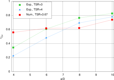
(a) $r_{C_{P}}$

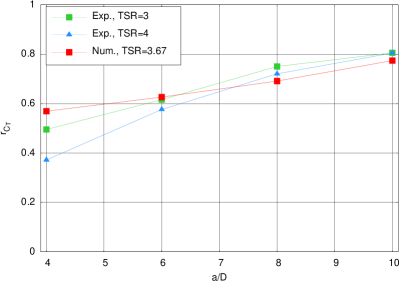
(b) $r_{C_{T}}$

Figure 12: Numerical comparison of $C_{P}$ and $C_{T}$ ratios for a given $TSR=TSR^{up}=TSR^{down}$.

Figure 12 depicts the evolution of these ratios $r_{C_{P}}$ and $r_{C_{T}}$ function of the inter-device distance $a$, for two experimental configurations and one numerical configuration. The comparison between numerical and experimental results show a good agreement, even if the discretisation is coarse and the results are not converged. This is promising for a future realistic turbine array numerical modelling.

4 Conclusions and outlook

A first study about interaction effects between two horizontal axis marine current turbines has been successfully carried out. On single device configurations, the wake behind the turbine was characterised in terms of velocity deficit and turbulence intensity, which showed that a higher upstream ambient TI tends to reduce the wake influence length. The behaviour of a single turbine has already been examined in terms of performance, which lead to determine that the range of TSR yielding the most power was between three and four for this type of blade geometry. These experimental data enabled the validation of the numerical tool both on the wake computation and on the performance evaluation. The comparison showed very promising results and we are confident that the software will soon be able to model successfully multi-device configurations (cf. figure 13). In addition, the numerical software is currently being rewritten in order to be more efficient and to include the latest numerical development such as a better turbulence model.

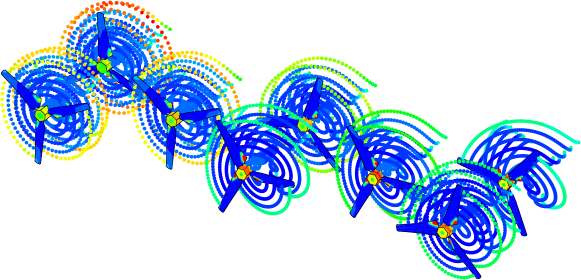
Figure 13: First coarse numerical simulation with eight turbines in close proximity.

Single configurations data have been used as a basis to carry out trials on two devices configurations. The study showed that wake interaction effects between the turbines exist and that the downstream turbine is thus deeply affected by the presence of an upstream device. A qualitative and quantitative characterization of the interaction has been presented concerning both the wake and the performance of the downstream turbine. It is clear that increasing inter-device spacing to retrieve higher individual power can only be done to the detriment of the total number of turbine rows in a given space. So a compromise between individual performance and the number of energy converters has to be made wisely when considering an array implantation.

Some of our prospects, which concern both the experimental and the numerical aspect, consist in modelling other kinds of turbine prototypes or in taking into account both wave and current effects on the behaviour of marine current turbines. Recently, new performance trials were run with a torque-meter instead of the load cell to measure the torque directly on the hub. In addition, twin-turbine configurations were tested in a flow with a 15% TI to complement the study presented here. Those results will be presented in [21, 20].

References

- Black [2011] R. Black, India plans asian tidal power first, News release, 2011. URL: http://www.bbc.co.uk/news/science-environment-12215065.
- Sco [2011] ScottishPower renewables receives consent to develop the world’s first tidal power array in the Sound of Islay, Press release, 2011. URL: http://www.scottishpowerrenewables.com/pages/press_releases.asp?article=98&date_year=2011.
- MCT [2011] Marine current turbines kicks off first tidal array for Wales, News release, 2011. URL: http://www.marineturbines.com/3/news/article/44/marine_current_turbines_kicks_off_first_tidal_array_for_wales.
- Bahaj and Myers [2004] A. S. Bahaj, L. Myers, Analytical estimates of the energy yield potential from the alderney race (channel islands) using marine current energy converters, Renewable Energy 29 (2004) 1931–1945.
- Batten et al. [2008] W. Batten, A. Bahaj, A. Molland, J. Chaplin, The prediction of the hydrodynamic performance of marine current turbines, Renewable Energy 33 (2008) 1085–1096.
- Baltazar and Falcão de Campos [2008] J. Baltazar, J. A. C. Falcão de Campos, Hydrodynamic analysis of a horizontal axis marine current turbine with a boundary element method, in: Proceedings of the ASME 27th Conference on Offshore Mechanics and Arctic Engineering (OMAE), ASME, 2008, pp. 883–893. URL: http://link.aip.org/link/abstract/ASMECP/v2008/i48234/p883/s1. doi:10.1115/OMAE2008-58033, Estoril, Portugal.
- Maganga et al. [2010] F. Maganga, G. Germain, J. King, G. Pinon, E. Rivoalen, Experimental characterisation of flow effects on marine current turbine behaviour and on its wake properties, IET Renewable Power Generation 4 (2010) 498–509.
- Myers et al. [2010] L. Myers, A. Bahaj, C. Retzler, P. Ricci, J.-F. Dhedin, Inter-device spacing issues within wave and tidal energy converter arrays., in: 3rd International Conference on Ocean Energy, 2010.
- Rawlinson-Smith et al. [2010] R. Rawlinson-Smith, I. Bryden, M. Folley, V. Martin, T. Stallard, C. Stock-Williams, R. Willden, The perawat project: Performance assessment of wave and tidal array systems, in: 3rd International Conference on Ocean Energy, 2010.
- Li and Calisal [2011] Y. Li, S. M. Calisal, Modeling of twin-turbine systems with vertical axis tidal current turbine: Part II–torque fluctuation, Ocean Engineering 38 (2011) 550–558.
- Pinon et al. [2012] G. Pinon, P. Mycek, G. Germain, E. Rivoalen, Numerical simulation of the wake of marine current turbines with a particle method, Renewable Energy 46 (2012) 111 – 126.
- Leonard [1980] A. Leonard, Vortex methods for flow simulation, Journal of Computational Physics 37 (1980) 289–335.
- Winckelmans and Leonard [1993] G. S. Winckelmans, A. Leonard, Contributions to vortex particle methods for the computation of three-dimensional incompressible unsteady flows, Journal of Computational Physics 109 (1993) 247–273.
- Cottet and Koumoutsakos [2000] G. Cottet, P. Koumoutsakos, Vortex methods: theory and practice, Cambridge University Press, 2000.
- Zervos et al. [1988] A. Zervos, S. Huberson, A. Hemon, Three-dimensional free wake calculation of wind turbine wakes, Journal of Wind Engineering and Industrial Aerodynamics 27 (1988) 65–76.
- Huberson et al. [2008] S. Huberson, E. Rivoalen, S. Voutsinas, Vortex particle methods in aeroacoustic calculations, Journal of Computational Physics 227 (2008) 9216–9240. Special Issue Celebrating Tony Leonard’s 70th Birthday.
- Pinon et al. [2005] G. Pinon, H. Bratec, S. Huberson, G. Pignot, E. Rivoalen, Vortex method for simulation of a 3d round jet in a cross-stream, Journal of Turbulence 6 (2005) 1–25.
- Bahaj et al. [2007] A. Bahaj, W. Batten, G. McCann, Experimental verifications of numerical predictions for the hydrodynamic performance of horizontal axis marine current turbines, Renewable Energy 32 (2007) 2479–2490.
- Meneveau and Katz [2000] C. Meneveau, J. Katz, Scale-invariance and turbulence models for large-eddy simulation, Annual Review of Fluid Mechanics 32 (2000) 1–32.
- Mycek et al. [2013a] P. Mycek, B. Gaurier, G. Germain, G. Pinon, E. Rivoalen, Experimental study of the turbulence intensity effects on marine current turbines behaviour. Part II: two interacting turbines, Submitted to Renewable Energy (2013a).
- Mycek et al. [2013b] P. Mycek, B. Gaurier, G. Germain, G. Pinon, E. Rivoalen, Experimental study of the turbulence intensity effects on marine current turbines behaviour. Part I: one single turbine, Submitted to Renewable Energy (2013b).