Laplacian Spectral Properties of Graphs from Random Local Samples

Abstract

The Laplacian eigenvalues of a network play an important role in the analysis of many structural and dynamical network problems. In this paper, we study the relationship between the eigenvalue spectrum of the normalized Laplacian matrix and the structure of ‘local’ subgraphs of the network. We call a subgraph local when it is induced by the set of nodes obtained from a breath-first search (BFS) of radius $r$ around a node. In this paper, we propose techniques to estimate spectral properties of the normalized Laplacian matrix from a random collection of induced local subgraphs. In particular, we provide an algorithm to estimate the spectral moments of the normalized Laplacian matrix (the power-sums of its eigenvalues). Moreover, we propose a technique, based on convex optimization, to compute upper and lower bounds on the spectral radius of the normalized Laplacian matrix from local subgraphs. We illustrate our results studying the normalized Laplacian spectrum of a large-scale online social network.

1 Introduction

Understanding the relationship between the structure of a network and its eigenvalues is of great relevance in the field of network science (see [3], [16] and references therein). The growing availability of massive databases, computing facilities, and reliable data analysis tools has provided a powerful framework to explore this relationship for many real-world networks. On the other hand, in many cases of practical interest, one cannot efficiently retrieve and/or store the exact full topology of a large-scale network. Alternatively, it is usually easy to retrieve local samples of the network structure. In this paper, we focus our attention on local sample of the network structure given in the form of a subgraph induced by the set of nodes obtained from a breath-first search (BFS) of small radius $r$ around a particular node.

We study the relationship between the normalized Laplacian spectrum of a graph and a random collection of local subgraphs. We show how local structural information contained in these localized subgraphs can be efficiently aggregated to infer global properties of the normalized Laplacian spectrum. Our analysis reveals that certain spectral properties, such as the so-called spectral moments (the power-sums of the eigenvalues), can be efficiently estimated from a random collection of localized subgraphs. Furthermore, applying recent results connecting the classical moment problem and convex optimization, we propose a series of semidefinite programs (SDP) to compute upper and lower bounds on the Laplacian spectral radius from a collection of local structural samples.

1.1 Previous Work

Studying the relationship between the structure of a graph and its eigenvalues is the central topic in the field of algebraic graph theory [1],[3],[5],[12]. In particular, the spectrum of the Laplacian matrix has a direct connection to the behavior of several networked dynamical processes, such as random walks [10], consensus dynamics [16], and a wide variety of distributed algorithms [11].

In many cases of practical interest it is unfeasible to exactly retrieve the complete structure of a network of contacts, making it impossible to compute the graph spectrum directly. However, in most cases one can easily retrieve local subgraphs obtained via BFS of small radius. To estimate spectral properties from localized structural samples, researchers have proposed a variety of random network models in which they can prescribe features retrieved from these samples, such as the degree distribution [4],[15], local correlations [13],[17], or clustering [14].

Although random networks are the primary tool to study the impact of local structural features on spectral network properties [4], this approach presents a major flaw: Random network models implicitly induce structural properties that are not directly controlled in the model construction, but can have a strong influence on the eigenvalue spectrum. For example, it is possible to find two networks having the same degree distribution, but with very different eigenvalue spectra.

1.2 Our contribution

In this paper, we develop a mathematical framework, based on algebraic graph theory and convex optimization, to study how localized samples of the network structure can be used to compute spectral properties of the normalized Laplacian matrix of (possibly weighted) graphs. The following are our main contributions:

• We develop a sublinear time algorithm to estimate the spectral moments (power-sums of the eigenvalues) of the normalized Laplacian matrix of a graph from a random set of local subgraphs samples. In our analysis, we use Hoeffding inequality to provide quality guarantees of our estimators as a function of the number of samples.

• We provide a convex program to compute, in linear time, upper and lower bounds on the Laplacian spectral radius from a random set of local subgraph samples. Our results are based on recent results connecting the classical moment problem with semidefinite programs (SDP).

2 Problem Formulation.

2.1 Notation and Preliminaries.

Let $\mathcal{G}:=(\mathcal{V},\mathcal{E})$ be an undirected unweighted graph (or network), where $\mathcal{V}:=\{v_{1},v_{2},...v_{n}\}$ represents the set of nodes and $\mathcal{E}\subseteq\mathcal{V}\times\mathcal{V}$ represents the set of edges. The neighborhood of $v_{i}\in\mathcal{V}$ is defined as $\mathcal{N}_{i}:=\{v_{j}\in\mathcal{V}:\{v_{i},v_{j}\}\in\mathcal{E}\}$. The degree of node $v_{i}$ is $d_{i}:=|\mathcal{N}_{i}|$. A weighted graph is defined as the triad $\mathcal{H}:=(\mathcal{V},\mathcal{E},\mathcal{W})$, where $\mathcal{W}$ is a weight function $\mathcal{W}:\mathcal{E}\to\mathbb{R}_{+}$ that assigns a real positive weight to each edge in $\mathcal{E}$. We define the weight coefficient as $w_{ij}:=\mathcal{W}(\{v_{i},v_{j}\})$ if $\{v_{i},v_{j}\}\in\mathcal{E}$, and $w_{ij}=0$ otherwise. The weighted degree of node $v_{i}$ in a weighted graphs is defined as $d_{i}^{\mathcal{H}}:=\sum_{j=1}^{n}w_{ij}$.

A walk of length $k$ from node $v_{i_{0}}$ to $v_{i_{k}}$ is defined as an ordered sequence of vertices $p:=(v_{i_{0}},v_{i_{1}},\ldots,v_{i_{k}})$, where $\{v_{i_{l}},v_{i_{l+1}}\}\in\mathcal{E}$, $l=0,1,\ldots,k-1$. If $v_{i_{0}}=v_{i_{k}}$, the walk is said to be closed. Given a walk $p=(v_{i_{0}},v_{i_{1}},\ldots,v_{i_{k}})$ in a weighted graph $\mathcal{H}$, its weight is defined as the product of the edge weights, $\omega_{\mathcal{H}}(p):=w_{i_{0}i_{1}}w_{i_{1}i_{2}}....w_{i_{k-1}i_{k}}$. The distance $\delta_{ij}$ between nodes $v_{i}$ and $v_{j}$ is defined as the minimum number of hops from $v_{i}$ to $v_{j}$.

The adjacency matrix of an unweighted network $\mathcal{G}$ is defined as the $n\times n$ Boolean symmetric matrix $A_{\mathcal{G}}:=[a_{ij}]$, defined entry-wise as $a_{ij}=1$ if $v_{i}$ is connected to $v_{j}$, and $a_{ij}=0$ otherwise. The adjacency matrix of a weighted graph $\mathcal{H}$ is defined as the symmetric matrix $W_{\mathcal{H}}:=[w_{ij}]$, where $w_{ij}$ are the weight coefficients. The degree matrix of a weighted graph $\mathcal{H}$ is the diagonal matrix of its weighted degrees, i.e., $D_{\mathcal{H}}=\mbox{diag}(d_{i}^{\mathcal{H}})$. The normalized Laplacian matrix of a weighted graph $\mathcal{H}$ is defined as

(2.1) $$L_{\mathcal{H}}:=I-D_{\mathcal{H}}{}^{-1/2}W_{\mathcal{H}}D_{\mathcal{H}}{}^{-1/2}.$$

The normalized Laplacian $L_{\mathcal{H}}$ is a symmetric, positive semidefinite matrix [3]. Thus, it has $n$ nonnegative eigenvalues $\lambda_{1}\geq\lambda_{2}\geq\ldots\geq\lambda_{n}\geq 0$ and a full set of orthogonal eigenvectors $v_{1},\ldots,v_{n}$. The largest eigenvalue $\lambda_{1}$ is called the spectral radius of $L_{\mathcal{H}}$, which satisfies $\lambda_{1}\leq 2$, [3]. Given a $n\times n$ symmetric matrix $M$ with (real) eigenvalues $\nu_{1},\ldots,\nu_{n}$, we define the $k$-th spectral moment of $M$ as

(2.2) $$m_{k}(M):=\frac{1}{n}\sum\limits_{i=1}^{n}\nu_{i}^{k}.$$

We now provide graph-theoretical elements to characterize the information contained in local subgraphs of the network. Given a weighted graph $\mathcal{H}$, we define the $r$-th order neighborhood around node $v_{i}$ as the subgraph $\mathcal{H}_{i,r}=(\mathcal{N}_{i,r},\mathcal{E}_{i,r},\mathcal{W})$ with node-set $\mathcal{N}_{i,r}:=\left\{v_{j}\in\mathcal{V}:\delta_{i,j}\leq r\right\}$ and edge-set $\mathcal{E}_{i,r}:=\{\left\{v,w\right\}\in\mathcal{E}$ s.t. $v,w\in\mathcal{N}_{i,r}\}$. Notice that $\mathcal{H}_{i,r}$ is the subgraph of $\mathcal{H}$ induced by the set of nodes that are at a distance $r$ or less from $v_{i}$. This set of nodes can be found using a BFS of radius $r$ starting at node $v_{i}$. Motivated by this interpretation, we call $\mathcal{H}_{i,r}$ the egonet of radius $r$ around node $v_{i}$. Egonets can be algebraically represented via submatrices of the weighted adjacency matrix $W_{\mathcal{H}}$, as follows. Given a set of $k$ nodes $\mathcal{K}\subseteq\mathcal{V}$, we denote by $W_{\mathcal{H}}\left(\mathcal{K}\right)$ the $k\times k$ submatrix of $W_{\mathcal{H}}$ formed by selecting the rows and columns of $W_{\mathcal{H}}$ indexed by $\mathcal{K}$. In particular, given the egonet $\mathcal{H}_{i,r}$, we define its adjacency matrix as $W_{i,r}(\mathcal{H}):=W_{\mathcal{H}}\left(\mathcal{N}_{i,r}\right)$. By convention, we associate the first row and column of the submatrix $W_{i,r}$ with node $v_{i}\in\mathcal{V}$ (the ‘center’ of the egonet), which can be done via a simple permutation of $W_{i,r}$.

2.2 Problem Statement.

The Laplacian eigenvalues of a graph can be efficiently computed for graphs of small and medium size. In graphs of large size, this computation is much more challenging. Furthermore, in many real-world networks, one cannot retrieve the complete network structure due to, for example, privacy and/or security constrains (e.g. Facebook). Alternatively, it is usually easy to retrieve local samples of the graph structure in the form of egonets. For example, one can acquire information about the network structure by extracting egonets of radius $r$ around a random sample of nodes. Therefore, it is realistic to assume that one does not have access to the complete topology of a large-scale network; instead, one can access only a (relatively small) number of egonets in the network.

Clearly, egonets do not completely describe the network structure; thus, it is impossible to compute exactly the graph spectrum from local egonets. In this paper, we show that, despite this limitation, we are able to compute many spectral graph properties from the egonets. We show that given a (sufficiently large) random collection of egonets of radius $r$, one can efficiently estimate the spectral moments of the normalized Laplacian matrix, $m_{k}(L_{\mathcal{H}})$, for $k\leq 2r+1$. Furthermore, we show that, given a truncated sequence of spectral moments, one can derive bounds on relevant spectral properties, such as the spectral radius of the Laplacian. As part of our analysis, we provide quality guarantees for all the estimators and bounds herein proposed.

3 Spectral Moments for Random Egonets

We start our analysis assuming the (unrealistic) situation in which one can access all the egonets in the network. Under this assumption, we shall derive expressions for the spectral moments of the normalized Laplacian matrix. Afterwards, we shall relax our assumptions and consider the more realistic case in which one can only access a (relatively small) number of random egonets. In this case, we propose estimators for the spectral moments and analyze their quality using Hoeffding inequality.

3.1 Spectral Moments as Averages.

We derive an expression for the $k$-th spectral moments of the normalized Laplacian matrix of a weighted graph, $L_{\mathcal{H}}$, from local egonets of radius $r$, $\mathcal{H}_{i,r}$. In our derivations, we use the following lemma from algebraic graph theory [1]:

Lemma 3.1

Let $\mathcal{H}$ be an undirected, weighted graph with adjacency matrix $W_{\mathcal{H}}=[w_{ij}]$, then

(3.3) $$\left[W_{\mathcal{H}}^{k}\right]_{ii}=\sum_{p\in P_{i,k}}\omega_{\mathcal{H}}(p),$$

where $\left[W_{\mathcal{H}}^{k}\right]_{ii}$ is the $\left(i,i\right)$-th entry of the $k$-th power of the adjacency $W_{\mathcal{H}}$ and $P_{i,k}$ is the set of all closed walks of length $k$ starting and finishing at node $v_{i}$.

Using Lemma 3.1, we can compute the spectral moments of the weighted adjacency matrix $W_{\mathcal{H}}$, as follows:

Theorem 3.1

Consider a weighted, undirected graph $\mathcal{H}$ with adjacency matrix $W_{\mathcal{H}}$. Let $W_{i,r}(\mathcal{H})$ be the (weighted) adjacency matrix of the egonet of radius $r$ around node $v_{i}$, $\mathcal{H}_{i,r}$. Then, the spectral moments of $W_{\mathcal{H}}$ can be written as

(3.4) $$m_{k}\left(W_{\mathcal{H}}\right)=\frac{1}{n}\sum_{i=1}^{n}\left[W_{i,r}^{k}\left(\mathcal{H}\right)\right]_{11},$$

for $k\leq 2r+1$.

• Since the trace of a matrix is the sum of its eigenvalues, we can expand the $k$-th spectral moment of the adjacency matrix as follows:

  (3.5) $$m_{k}\left(W_{\mathcal{H}}\right)=\frac{1}{n}\text{Trace}\left(W_{\mathcal{H}}^{k}\right)=\frac{1}{n}\sum_{i=1}^{n}\left[W_{\mathcal{H}}^{k}\right]_{ii}.$$

  From Lemma 3.1, we have that $\left[W_{\mathcal{H}}^{k}\right]_{ii}=\sum_{p\in P_{k,i}}\omega_{\mathcal{H}}(p)$. Notice that for a fixed value of $k$, closed walks of length $k$ in $\mathcal{H}$ starting at node $v_{i}$ can only touch nodes within a certain distance $r\left(k\right)$ of $v_{i}$, where $r\left(k\right)$ is a function of $k$. In particular, for $k$ even (resp. odd), a closed walk of length $k$ starting at node $i$ can only touch nodes at most $k/2$ (resp. $\left\lfloor k/2\right\rfloor$) hops away from $v_{i}$. Therefore, closed walks of length $k$ starting at $v_{i}$ are always contained within the neighborhood of radius $\left\lfloor k/2\right\rfloor$. In other words, the egonet $\mathcal{H}_{i,r}$ of radius $r$ contains all closed walks of length up to $2r+1$ starting at node $v_{i}$. We can count these walks by applying Lemma 3.1 to the local adjacency matrix $W_{i,r}$. In particular, $\sum_{p\in P_{k,i}}\omega_{\mathcal{H}}(p)$ is equal to $\left[W_{i,r}^{k}\left(\mathcal{H}\right)\right]_{11}$ (since, by convention, node $1$ in the local egonet $\mathcal{H}_{i,r}$ corresponds to node $i$ in the graph $\mathcal{H}$). Therefore, for $k\leq 2r+1$, we have that

  (3.6) $$\left[W_{i,r}^{k}\left(\mathcal{H}\right)\right]_{11}=\sum_{p\in P_{k,i}}\omega_{\mathcal{H}}(p)=\left[W_{\mathcal{H}}^{k}\right]_{ii}.$$

  Then, substituting (3.6) into (3.5), we obtain the statement of our Theorem.

The above theorem allows us to compute a truncated sequence of spectral moments $\left\{m_{k}\left(W_{\mathcal{H}}\right)\text{, }k\leq 2r+1\right\}$, given all the egonets of radius $r$, $\left\{\mathcal{H}_{i,r}\text{, }v_{i}\in\mathcal{V}\right\}$. According to (3.4), the $k$-th spectral moment is simply the average of the quantities $\left[W_{i,r}^{k}\left(\mathcal{H}\right)\right]_{11}$, $i=1,...,n$. For a fixed $k$, each value $\left[W_{i,r}^{k}\left(\mathcal{H}\right)\right]_{11}$, $i=1,\dots,n$, can be computed in time $O\left(\left|\mathcal{N}_{i,r}\right|^{3}\right)$, where $\left|\mathcal{N}_{i,r}\right|$ is the number of nodes in the local egonet $\mathcal{H}_{i,r}$. Notice that, if $\left|\mathcal{N}_{i,r}\right|=o\left(n\right)$, we can compute the $k$-th spectral moments in linear time (with respect to the size of the network) using (3.4).

In what follows, we use the above results to compute the spectral moments of the Laplacian matrix of a weighted graph, $L_{\mathcal{H}}$. Before we present our results, we define the so-called Laplacian graph:

Definition 3.1

Given a weighted graph $\mathcal{H}$, we define its Laplacian graph as $\mathcal{L}\left(\mathcal{H}\right):=\left(\mathcal{V},\mathcal{E\cup\widetilde{E}},\Pi\right)$, where $\mathcal{\widetilde{E}}:=\left\{\left\{v,v\right\}:v\in\mathcal{V}\right\}$ (the set of all self-loops), and the weight function $\Pi:\mathcal{E\cup\widetilde{E}}\to\mathbb{R}$ is defined as:

(3.7) $$\Pi\left(\left\{v_{i},v_{j}\right\}\right):=\left\{\begin{array}[]{ll}1,&\text{for }v_{i}=v_{j},\\ \frac{-w_{ij}}{\sqrt{d_{i}^{\mathcal{H}}d_{j}^{\mathcal{H}}}},&\text{for }\left\{v_{i},v_{j}\right\}\in\mathcal{E},v_{i}\neq v_{j}\\ 0,&\text{otherwise,}\end{array}\right.$$

where $d_{i}^{\mathcal{H}}$ is the weighted degree of node $v_{i}$ in $\mathcal{H}$.

Notice that the weighted adjacency matrix of the Laplacian graph $\mathcal{L}\left(\mathcal{H}\right)$, denoted by $W_{\mathcal{L}\left(\mathcal{H}\right)}$, is equal to the normalized Laplacian matrix of the weighted graph $\mathcal{H}$, $L_{\mathcal{H}}$. Thus, $m_{k}(L_{\mathcal{H}})=m_{k}\left(W_{\mathcal{L}(\mathcal{H})}\right)$ and we can compute the spectral moments of the normalized Laplacian matrix using weighted walks in the Laplacian graph. In particular, the Laplacian spectral moments satisfy

(3.8) $$m_{k}(L_{\mathcal{H}}) = m_{k}\left(W_{\mathcal{L}(\mathcal{H})}\right)$$

$$= \frac{1}{n}\sum_{i=1}^{n}\left[W_{\mathcal{L\left(H\right)}}^{k}\right]_{ii}$$

$$= \frac{1}{n}\sum_{i=1}^{n}\left[W_{i,r}^{k}\left(\mathcal{L\left(H\right)}\right)\right]_{11}$$

where $\left[W_{i,r}^{k}\left(\mathcal{L\left(H\right)}\right)\right]_{11}$ is the $\left(1,1\right)$-th entry of the $k$-th power of the weighted adjacency matrix representing the egonet of radius $r$ around node $v_{i}$ in the Laplacian graph $\mathcal{L\left(H\right)}$. Notice that $\left[W_{i,r}^{k}\left(\mathcal{L\left(H\right)}\right)\right]_{11}$ is a real number that depends solely on the structure of the egonet $W_{i,r}(\mathcal{H})$; thus, it is a variable that can be computed using local information about the structure of the network around node $v_{i}$.

In theory, if we had access to all the egonets in the graph, we could calculate $W_{i,r}^{k}\left(\mathcal{L\left(H\right)}\right)$ for all $v_{i}\in\mathcal{V}$, and compute the spectral moments of the Laplacian matrix in linear time (under certain sparsity assumptions). However, it is often impractical to traverse all the egonets of a real-world large-scale network because of high computational cost. In the following subsection, we introduce a method to approximate the spectral moments of a network in sublinear time from a random collection of $s$ egonets and analyze the quality of our approximation as a function of $s$.

3.2 Sampling Egonets and Moment Estimation.

Define the following ‘local’ variable

(3.9) $$\phi_{i,r}^{\left(k\right)}:=\left[W_{i,r}^{k}\left(\mathcal{L\left(H\right)}\right)\right]_{11},k\leq 2r+1.$$

Notice that $\phi_{i,r}^{\left(k\right)}$ is a function of the egonet of radius $r$ around node $v_{i}$, since $W_{i,r}\left(\mathcal{L\left(H\right)}\right)$ is the weighted adjacency matrix of the egonet in the Laplacian graph. Thus, $\phi_{i,r}^{\left(k\right)}$ is a local variable associated to the $r$-th neighborhood around node $v_{i}$. According to (3.8), the $k$-th Laplacian spectral moment can be computed as the average,

$$m_{k}(L_{\mathcal{H}})=\frac{1}{n}\sum_{i=1}^{n}\phi_{i,r}^{\left(k\right)},$$

Let us now assume that we do not have access to $\phi_{i,r}^{\left(k\right)}$, for all $v_{i}\in\mathcal{V}$; instead, we only have access to $\phi_{i,r}^{\left(k\right)}$ for $v_{i}\in\mathcal{S}$, where $\mathcal{S}\subset\mathcal{V}$ is a subset of randomly sampled nodes. Since the spectral moment is a global average, we propose the following estimator of $m_{k}(L_{\mathcal{H}})$:

(3.10) $$\widetilde{m}_{k}(L_{\mathcal{H}}):=\frac{1}{\left|\mathcal{S}\right|}\sum_{v_{i}\in\mathcal{S}}\phi_{i,r}^{\left(k\right)}.$$

In what follows, we establish the quality of this estimator using Chernoff-Hoeffding inequality.

Lemma 3.2

(Hoeffding Inequality) Let $X_{1},X_{2},\ldots,X_{k}$ be independent random variables with $P(X_{i}\in[a,b])=1$ for $1\leq i\leq k$. Define the mean of these variables as $\overline{X}=\frac{1}{k}\sum_{i=1}^{k}X_{i}$, then for any positive $t$, the following inequality holds

(3.11) $$Pr\{\left|\overline{X}-\mathbb{E}(\overline{X})\right|\geq t\}\leq 2\exp\left(\frac{-2kt^{2}}{(b-a)^{2}}\right),$$

where $\mathbb{E}(\overline{X})$ is the expected value of $\overline{X}$.

In order to apply the above lemma, we need the following result:

Lemma 3.3

The variable $\phi_{i,r}^{\left(k\right)}$ satisfies $0\leq\phi_{i,r}^{\left(k\right)}\leq 2^{k-1}$ for all $i\in\left[n\right]$, $k\geq 1$.

• Let $\lambda_{i}$ and $\mathbf{v}_{i}$ denote the eigenvalues and eigenvectors of the Laplacian matrix $L_{\mathcal{H}}$, for $i=1,2,\ldots,n$. Since $L_{\mathcal{H}}$ is symmetric is always diagonalizable and it has a complete set of orthonormal eigenvectors. Furthermore, $L_{\mathcal{H}}$ is also positive semidefinite; thus, its eigenvalues are nonnegative. Define the matrix $V$ whose columns are the eigenvectors $\mathbf{v}_{i}$, and the diagonal matrix $\Lambda=\mbox{diag}(\lambda_{1},\lambda_{2}...,\lambda_{n})$. Then, $L_{\mathcal{H}}=V\Lambda V^{T}$, and

  (3.12) $$L_{\mathcal{H}}^{k}=V\Lambda^{k}V^{T}=\sum\limits_{j=1}^{n}\lambda_{j}^{k}\mathbf{v}_{j}\mathbf{v}_{j}^{T}.$$

  Denoting the $i$-th element of vector $\mathbf{v}_{j}$ as $v_{j,i}$, we have

  (3.13) $$[L_{\mathcal{H}}^{k}]_{ii}=\sum\limits_{j=1}^{n}\lambda_{j}^{k}v_{j,i}^{2}.$$

  From (2.1), we have that $[L_{\mathcal{H}}]_{ii}=1$. Thus,

  (3.14) $$[L_{\mathcal{H}}]_{ii}=\sum\limits_{j=1}^{n}\lambda_{j}v_{j,i}^{2}=1.$$

  According to [3], the eigenvalues satisfy $0\leq\lambda_{i}\leq 2$ for any $i\in\left[n\right]$. Thus,

  $$[L_{\mathcal{H}}^{k}]_{ii} = \sum\limits_{j=1}^{n}\lambda_{j}v_{j,i}^{2}\cdot\lambda_{j}^{k-1}$$

  $$\leq \left(\sum\limits_{j=1}^{n}\lambda_{j}v_{j,i}^{2}\right)\lambda_{1}^{k-1}$$

  $$\leq \left(\sum\limits_{j=1}^{n}\lambda_{j}v_{j,i}^{2}\right)2^{k-1}$$

  $$= 2^{k-1},$$

  where we have used the fact that $2\geq\lambda_{1}\geq\lambda_{i}$, for all $i$. Also, notice from (3.13), that every element in the summation is nonnegative, then $[L_{\mathcal{H}}^{k}]_{ii}$ is nonnegative.

From Lemmas 3.3 and 3.2, we obtain the following quality guarantee on our estimator:

Theorem 3.2

Consider a set $\mathcal{S}\subset\mathcal{V}$ of nodes chosen uniformly at random. Then, the estimator $\widetilde{m}_{k}(L_{\mathcal{H}})$ for the $k$-th Laplacian spectral moment defined in (3.10) satisfies

$$\Pr\left\{\left|\widetilde{m}_{k}(L_{\mathcal{H}})-m_{k}(L_{\mathcal{H}})\right|\geq t_{k}\right\}\leq 2\exp\left(\frac{-8t_{k}^{2}\left|\mathcal{S}\right|}{4^{k}}\right).$$

• The proof is a direct application of Lemma 3.2 after substituting $\phi_{i,r}^{\left(k\right)}$ for $X_{i}$ and $\left[0,2^{k-1}\right]$ for $\left[a,b\right]$. Using this result, we can calculate the number of samples $\left|\mathcal{S}\right|$ needed to achieve a particular error in our moment estimation with a given probability. For each value of $k$, we denote by $s_{k}$ the sample size needed to achieve an error $t_{k}$ with a probability less or equal to $\delta_{k}=2\exp\Big{(}\frac{-8t_{k}^{2}s_{k}}{4^{k}}\Big{)}$. Let us define the normalized error $\varepsilon_{k}:=\frac{t_{k}}{2^{k-1}}$, then taking $s_{k}=\frac{1}{2}\varepsilon_{k}^{-2}\ln\frac{2}{\delta_{k}}$ samples, we achieve an error $t_{k}$ with probability at most $\delta_{k}$, i.e., $\Pr\left\{\left|\widetilde{m}_{k}(L_{\mathcal{H}})-m_{k}(L_{\mathcal{H}})\right|\geq t_{k}\right\}\leq\delta_{k}$.

4 Moment-Based Spectral Analysis.

Using Theorem 3.1, we can get a truncated sequence of approximated spectral moments of the Laplacian matrix $L_{\mathcal{H}}$, $\left\{m_{k}(L_{\mathcal{H}})\right\}_{k\leq 2r+1}$, from a set of local egonets of radius $r$. We now present a convex optimization framework to extract information about the largest eigenvalue of the weighted adjacency matrix, $\lambda_{1}\left(L_{\mathcal{H}}\right)$, from this sequence of moments.

4.1 Moment-Based Spectral Bounds

We can state the problem solved in this subsection as follows:

Problem. Given a truncated sequence of Laplacian spectral moments $\left\{m_{k}(L_{\mathcal{H}})\right\}_{k\leq 2r+1}$, find tight upper and lower bounds on the largest eigenvalue $\lambda_{1}\left(L_{\mathcal{H}}\right)$.

Our approach is based on a probabilistic interpretation of the eigenvalue spectrum of a given network. To present our approach, we first need to introduce some concepts:

Definition 4.1

Given a weighted, undirected Laplacian matrix $L_{\mathcal{H}}$ with (real) eigenvalues $\lambda_{1},...,\lambda_{n}$, the Laplacian spectral density is defined as,

(4.15) $$\mu_{L_{\mathcal{H}}}\left(x\right)\triangleq\frac{1}{n}\sum_{i=1}^{n}\delta\left(x-\lambda_{i}\right),$$

where $\delta\left(\cdot\right)$ is the Dirac delta function.

The spectral density can be interpreted as a discrete probability density function with support on the set of eigenvalues $\left\{\lambda_{i},\text{ }i=1...n\right\}$. Let us consider a discrete random variable $X$ whose probability density function is $\mu_{L_{\mathcal{H}}}$. The moments of this random variable satisfy the following [19]:

$$\mathbb{E}_{\mu_{L_{\mathcal{H}}}}\left(X^{k}\right)=m_{k}\left(L_{\mathcal{H}}\right),$$

for all $k\geq 0$.

We now present a convex optimization framework that allows us to find bounds on the endpoints of the smallest interval $\left[a,b\right]$ containing the support of a generic random variable $X\sim\mu$ given a sequence of moments $\left(M_{0},M_{1},...,M_{2r+1}\right)$, where $M_{k}\triangleq\int x^{k}dx$. Subsequently, we shall apply these results to find bounds on $\lambda_{1}\left(L_{\mathcal{H}}\right)$. Our formulation is based on the following matrices:

Definition 4.2

Given a sequence of moments $\mathbf{M}_{2r+1}=\left(M_{0},M_{1},...,M_{2r+1}\right)$, let $H_{2r}\left(\mathbf{M}_{2r+1}\right)$ and $H_{2r+1}\left(\mathbf{M}_{2r+1}\right)\in\mathbb{R}^{\left(r+1\right)\times\left(r+1\right)}$ be the Hankel matrices defined by:

(4.16) $$\left[H_{2r}\right]_{ij}\triangleq M_{i+j-2}, \left[H_{2r+1}\right]_{ij}\triangleq M_{i+j-1}.$$

The above matrices are called the moment matrices associated with the sequence $\mathbf{M}_{2r+1}$.

Given a truncated sequence of moments of a probability distribution, we can compute a bound on its support as follows [8][7]:

Theorem 4.1

Let $\mu$ be a probability density function on $\mathbb{R}$ with associated sequence of moments $\mathbf{M}_{2r+1}=\left(M_{0},M_{1},...,M_{2r+1}\right)$, all finite, and let $\left[a,b\right]$ be the smallest interval which contains the support of $\mu$. Then, $b\geq\beta^{\ast}\left(\mathbf{M}_{2r+1}\right)$, where

(4.17) $$\begin{array}[]{rrl}\beta_{r}^{\ast}\left(\mathbf{M}_{2r+1}\right):=&\min_{x}&x\\ &\text{s.t.}&H_{2r}\succeq 0,\\ &&x~{}H_{2r}-H_{2r+1}\succeq 0.\end{array}$$

Observe that, for a given sequence of moments $\mathbf{M}_{2r+1}$, the entries of $xH_{2r}-H_{2r+1}$ depend affinely on the variable $x$. Then $\beta^{\ast}\left(\mathbf{m}_{2r+1}\right)$ is the solutions to a semidefinite program (SDP) in one variable. Hence, $\beta^{\ast}\left(\mathbf{M}_{2r+1}\right)$ can be efficiently computed using standard optimization software, e.g. [6], from a truncated sequence of moments.

Applying Theorem 4.1 to the spectral density $\mu_{L_{\mathcal{H}}}$ of a given graph $\mathcal{H}$ with spectral moments $\left(m_{0},m_{1},...,m_{2r+1}\right)$, we can find a lower bound on its largest eigenvalue, $\lambda_{1}\left(L_{\mathcal{H}}\right)$, as follows [19]:

Theorem 4.2

Let $L_{\mathcal{H}}$ be the normalized Laplacian matrix of a weighted, undirected graph with (real) eigenvalues $\lambda_{1}\geq...\geq\lambda_{n}$. Then, given a truncated sequence of the spectral moments of $L_{\mathcal{H}}$, $\mathbf{m}_{2r+1}=\left(m_{0},m_{1},\ldots,m_{2r+1}\right)$, we have that

(4.18) $$\lambda_{1}\left(L_{\mathcal{H}}\right)\geq\beta_{r}^{\ast}\left(\mathbf{m}_{2r+1}\right),$$

where $\beta_{r}^{\ast}\left(\mathbf{m}_{2r+1}\right)$ is the solution to the SDP in (4.17).

Using the optimization framework presented above, we can also compute upper bounds on the spectral radius of $\mathcal{H}$ from a sequence of its spectral moments, as follows. In this case, our formulation is based on the following set of Hankel matrices:

Definition 4.3

Given the Laplacian matrix of a weighted, undirected graph $L_{\mathcal{H}}$ with $n$ nodes and spectral moments $\mathbf{m}_{2r+1}=\left(m_{0},m_{1},...,m_{2r+1}\right)$, let $T_{2r}\left(y;\mathbf{m}_{2r+1},n\right)$ and $T_{2r+1}\left(y;\mathbf{m}_{2r+1},n\right)\in\mathbb{R}^{\left(r+1\right)\times\left(r+1\right)}$ be the Hankel matrices defined by:

(4.19) $$\left[T_{2r}\right]_{ij}:= \frac{n}{n-1}m_{i+j-2}-\frac{1}{n-1}y^{i+j-2},$$

(4.20) $$\left[T_{2r+1}\right]_{ij}:= \frac{n}{n-1}m_{i+j-1}-\frac{1}{n-1}y^{i+j-1}.$$

Given a sequence of spectral moments, we can compute upper bounds on the largest eigenvalue $\lambda_{1}\left(L_{\mathcal{H}}\right)$ using the following result [18][19]:

Theorem 4.3

Let $L_{\mathcal{H}}$ be the normalized Laplacian matrix of a weighted, undirected graph with (real) eigenvalues $\lambda_{1}\geq...\geq\lambda_{n}$. Then, given a truncated sequence of its Laplacian spectral moments $\mathbf{m}_{2r+1}=\left(m_{0},m_{1},...,m_{2r+1}\right)$, we have that

$$\lambda_{1}\leq\delta_{r}^{\ast}\left(\mathbf{m}_{2r+1},n\right),$$

where

(4.21) $$\begin{array}[]{rrl}\delta_{r}^{\ast}\left(\mathbf{m}_{2r+1},n\right):=&\max_{y}&y\\ &\text{s.t.}&T_{2r}\succeq 0,\\ &&yT_{2r}-T_{2r+1}\succeq 0,\\ &&T_{2r+1}\succeq 0.\end{array}$$

The optimization program in (4.21) is not an SDP, since the entries of the matrices $T_{2r}\left(y;\mathbf{m}_{2r+1},n\right)$ and $T_{2r+1}\left(y;\mathbf{m}_{2r+1},n\right)$ are not affine functions in $y$. Nevertheless, the program is clearly quasiconvex [2] and can be efficiently solved using a simple bisection algorithms.

In summary, using Theorems 3.1, 4.2, and 4.3, we can compute upper and lower bounds on the largest eigenvalue of the normalized Laplacian matrix of a weighted, undirected network, $\lambda_{1}\left(L_{\mathcal{H}}\right)$, from the set of local egonets with radius $r$, as follows: (Step 1) Using (3.4), compute the truncated sequence of moments $\left\{m_{k}(L_{\mathcal{H}})\right\}_{k\leq 2r+1}$ from the egonets, and (Step 2) using Theorems 4.2 and 4.3, compute the upper and lower bounds, $\delta_{r}^{\ast}\left(\mathbf{m}_{2r+1},n\right)$ and $\beta_{r}^{\ast}\left(\mathbf{m}_{2r+1}\right)$, respectively. However, the approach presented in this section is based on the assumption that we have access to all the egonets in the network. In Subsection 3.2, we have provided estimators of the spectral moments from a random sample of egonets. In the following subsection, we will illustrate how to use these estimators to derive upper and lower bounds on the Laplacian spectral radius from a random sample of egonets.

4.2 Bounds on Spectral Radius from Sampling Egonets

From Theorem 3.2, we have that the $k$-th Laplacian spectral moment $m_{k}=m_{k}\left(L_{\mathcal{H}}\right)$ satisfies

$$\Pr\left\{m_{k}\in[\widetilde{m}_{k}-t_{k},\widetilde{m}_{k}+t_{k}]\right\}\leq 2\exp\left(\frac{-8t_{k}^{2}\left|\mathcal{S}\right|}{4^{k}}\right),$$

where $\widetilde{m}_{k}=\widetilde{m}_{k}(L_{\mathcal{H}})$ was defined in (3.10). Then, the probability of a truncated sequence of moments $\left(m_{k}\right)_{k\leq 2r+1}$ satisfying $m_{k}\in[\widetilde{m}_{k}-t_{k},\widetilde{m}_{k}+t_{k}]$ for $k=2,\ldots,2r+1$, satisfies the following proposition (notice that $m_{1}=1$, for any $L_{\mathcal{H}}$):

Proposition 4.1

For a given $\Delta\in\left[0,1\right]$, we have that

$$\Pr\left(\bigcap_{k=2}^{2r+1}\left\{m_{k}\in[\widetilde{m}_{k}-t_{k},\widetilde{m}_{k}+t_{k}]\right\}\right)\geq\Delta,$$

if

(4.22) $$t_{k}=\frac{2^{k-1}}{\sqrt{2\left|\mathcal{S}\right|}}\ln^{1/2}\frac{4r}{1-\Delta}.$$

• First, we have that

  $$\Pr\left(\bigcap_{k=2}^{2r+1}\left\{m_{k}\in[\widetilde{m}_{k}-t_{k},\widetilde{m}_{k}+t_{k}]\right\}\right)$$

  $$= 1-\Pr\left(\bigcup_{k=2}^{2r+1}\left\{m_{k}\notin[\widetilde{m}_{k}-t_{k},\widetilde{m}_{k}+t_{k}]\right\}\right)$$

  $$\geq 1-\sum_{k=2}^{2r+1}\Pr\left(m_{k}\notin[\widetilde{m}_{k}-t_{k},\widetilde{m}_{k}+t_{k}]\right)$$

  $$\geq 1-2\sum_{k=2}^{2r+1}\exp\left(\frac{-8t_{k}^{2}\left|\mathcal{S}\right|}{4^{k}}\right).$$

  The last probability can be made equal to a desired $\Delta$ by choosing $t_{k}^{2}/4^{k}=\alpha$ for all $k=2,\ldots,2k+1$ with $\alpha$ satisfying $\Delta=1-4r\exp\left(-8\alpha\left|\mathcal{S}\right|\right)$. Or equivalently, $\alpha=\frac{1}{8\left|\mathcal{S}\right|}\ln\frac{4r}{1-\Delta}$, which implies the statement of the Proposition, after simple algebraic manipulations.

We can then apply the result in Theorem 4.2 to compute a probabilistic lower bound on the spectral radius by solving a modified version of the SDP in (4.17), as follows. First, given a sample set of nodes $\mathcal{S}$, we extract the corresponding egonets of radius $r$. Then, using (3.10) and (3.9), we compute a sequence of estimators $\widetilde{m}_{k}$ for $k=2,\ldots,2r+1$. Finally, according to Proposition 4.1, we modify the SDP in (4.17) to obtain our main result.

Theorem 4.4

Given a uniform sample set $\mathcal{S}\subset\mathcal{V}$ and the egonets of radius $r$ around the nodes in $\mathcal{S}$, the spectral radius of the normalized Laplacian matrix satisfies

$$\Pr\left(\lambda_{1}\left(L_{\mathcal{H}}\right)\geq\widetilde{\beta}_{r}\right)\geq\Delta,$$

where

$$\begin{array}[]{rrl}\widetilde{\beta}_{r}:=&\min_{x}&x\\ &\text{s.t.}&H_{2r}\succeq 0,\\ &&x~{}H_{2r}-H_{2r+1}\succeq 0,\\ &&\widetilde{m}_{k}-t_{k}\leq m_{k}\leq\widetilde{m}_{k}+t_{k},\\ &&k=2,\ldots,2r+1,\end{array}$$

with $m_{k}$ and $\widetilde{m}_{k}$ defined in (3.9) and (3.10), $H_{2r}$ and $H_{2r+1}$ defined in (4.16), and $t_{k}$ defined in (4.22).

The proof of the above theorem is a direct adaptation of Theorem 4.2 using Proposition 4.1. The same adaptation can be applied to derive an upper bound on the spectral radius of the normalized Laplacian matrix from Theorem 4.3 and Proposition 4.1.

5 Numerical Analysis

In this section, we will present the numerical analysis of spectral radius estimation, and verify the quality of estimation based on sampled nodes. In our simulations, we will use data from the Euro-Email network [9]. The network is composed of 36,692 nodes, which are connected by 183,831 edges. Here we consider the network as unweighted, undirected simple graph. Two nodes are connected as long as either user sent email to another. From the simple graph, we can construct the weighted Laplacian graph that corresponds to the simple graph.

To be able to compute the spectral radius, we extract a small network with 5000 nodes via BFS, so that we could compare the performance of sampling with the accurate computation. The subgraph with 5000 nodes will be the object of our analysis.

The nodes are assigned with indexes without consideration about their topology. To get a uniform sampling, the indexes are picked randomly, which compose the collection of sampled nodes.

In Figure 1, we take different number of samples from the network to estimate the bounds of the spectral radius based on egonet with radius $r_{0}=3$. In the simulation, the normalized error bound for the elements in the moment sequence is fixed, i.e. $\frac{t_{k}}{2^{k-1}}=0.08$. Here we assume that the moments for $k=1,2...5$ can be accurately computed, because it does not cost much to compute the power of the Laplacian matrix up to 5-th order. However, for the 6-th and 7-th moment, we take uniform samples from the whole network and approximate the moment using the estimator proposed in the previous sections, i.e. using average of the sampled egonets to approximate the global average. Thus for each $k>5$, $m_{k}\in[\widetilde{m_{k}}-t_{k},\widetilde{m_{k}}+t_{k}]$. With the size of the sampled nodes increasing, the quality (accuracy guarantee) of the estimator increases.

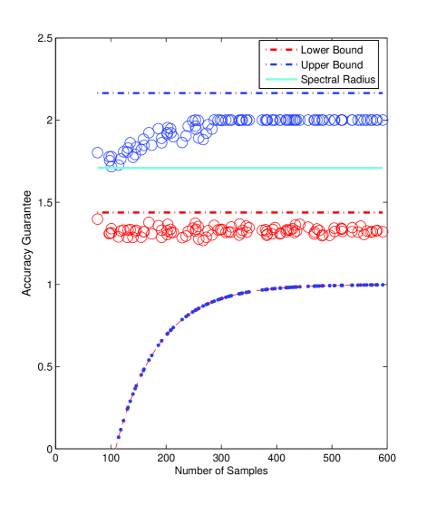
Figure 1: Estimation when the size of the samples varies. (1) The normalized error for each moment are the same. Samples with different sizes give different estimations of the bounds. (2) Quality guarantee is a function of the size of the sample. When the number of sample increases, the quality of the estimator increases.

From the upper part of the figure, it can be seen that the lower bound does not change much when the number of samples changes. For the upper bound, when the number of samples increases, the bound gets looser, but the accuracy guarantee that the spectral radius is within the bounds increase. The dotted lines are the bounds calculated by considering the egonets of every nodes in the network. And the circles are the estimated bounds when different sets of nodes are taken as samples. The lower part of Figure 1 gives the curve for the number of samples versus the accuracy guarantee. Though the network has 5000 nodes, taking 600 samples will give the estimation with nearly 100 percent.

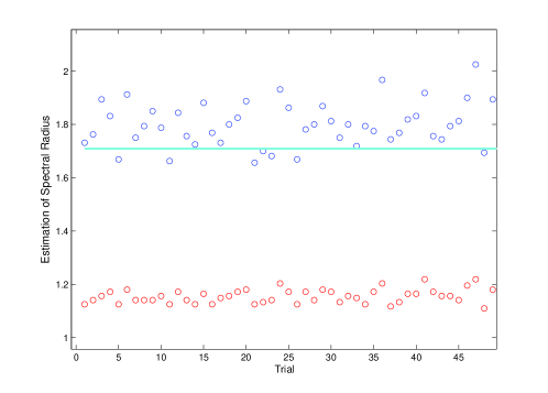
Figure 2: Spectral bounds for trials with the same sample size $\mathcal{S}=21$. When the number of samples are the same,

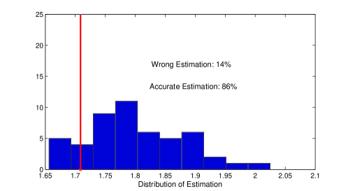
Figure 3: Distribution of estimation when the size of the sample is the same.

In Figure 2, we take different samples with the same sample size to verify the quality of estimation. The normalized error is set to be $\varepsilon_{k}=0.2$, and $\delta_{k}=0.4$, thus the sample size needed is $S=21$. From the figure, it can be seen that the lower bound is much loose, and almost the same when the sample pool are different. Checking whether the estimation range is correct for each trial, we can see from Figure 3 that the accuracy rate is $86\%$, which is much higher than the theoretical accuracy probability $1-\delta_{k}=0.6$.

6 Conclusion

In this paper, we apply graph theories and convex optimization techniques to study the spectrum property of the normalized Laplacian matrix. Instead of analyzing the whole network, we focus on localized structural features with radius $r$.

Due to the high cost of traversing all the nodes, we have proposed to take uniform samples from the network pool and use the sampled egonets to estimate the moments of the normalized Laplacian. With Hoeffding inequalities, we characterize the quality of the estimators in terms of normalized error and size of the sample. In addition, we have derived the lower and upper bounds of the spectral radius by solving a series of SDP problems, based on the collection of random subgraphs. The combination of quality guarantee of moment sequence and the optimization problems provides us with the estimation guarantee of the spectral radius.

References

- [1] N. Biggs, Algebraic Graph Theory, Cambridge University Press, 1993.
- [2] S. Boyd and L. Vandenberghe, Convex Optimization, Cambridge university press, 2004.
- [3] F. Chung, Spectral Graph Theory, vol. 92, AMS Bookstore, 1997.
- [4] F. Chung, L. Lu, and V. Vu, Spectra of random graphs with given expected degrees, Proceedings of the National Academy of Sciences, 100 (2003), pp. 6313–6318.
- [5] D. Cvetković, P. Rowlinson, and S. Simić, An Introduction to the Theory of Graph Spectra, Cambridge University Press Cambridge, 2010.
- [6] M. Grant, S. Boyd, and Y. Ye, Cvx: Matlab software for disciplined convex programming, 2008.
- [7] J.-B. Lasserre, Moments, Positive Polynomials and Their Applications, vol. 1, World Scientific, 2009.
- [8] , Bounding the support of a measure from its marginal moments, Proceedings of the American Mathematical Society, 139 (2011), pp. 3375–3382.
- [9] J. Leskovec, Stanford large network dataset collection. http://snap.stanford.edu/data/index.html.
- [10] L. Lovász, Random walks on graphs: A survey, Combinatorics, Paul erdos is eighty, 2 (1993), pp. 1–46.
- [11] N.A. Lynch, Distributed algorithms, Morgan Kaufmann, 1996.
- [12] B. Mohar and Y. Alavi, The laplacian spectrum of graphs, Graph theory, combinatorics, and applications, 2 (1991), pp. 871–898.
- [13] M. Newman, Assortative mixing in networks, Physical review letters, 89 (2002), p. 208701.
- [14] , Random graphs with clustering, Physical review letters, 103 (2009), p. 058701.
- [15] M. Newman, S. Strogatz, and D. Watts, Random graphs with arbitrary degree distributions and their applications, Physical Review E, 64 (2001), p. 026118.
- [16] R. Olfati-Saber, Flocking for multi-agent dynamic systems: Algorithms and theory, IEEE Transactions on Automatic Control, 51 (2006), pp. 401–420.
- [17] R. Pastor-Satorras, A. Vázquez, and A. Vespignani, Dynamical and correlation properties of the internet, Physical review letters, 87 (2001), p. 258701.
- [18] V.M Preciado and A. Jadbabaie, Moment-based spectral analysis of large-scale networks using local structural information, ACM/IEEE Transactions on Networking, 21 (2013), pp. 373–382.
- [19] V.M Preciado, A. Jadbabaie, and G.C. Verghese, Structural analysis of laplacian spectral properties of large-scale networks, IEEE Transactions on Automatic Control, 58 (2013), pp. 2338–2343.
- [20] L. Vandenberghe and S. Boyd, Semidefinite programming, SIAM review, 38 (1996), pp. 49–95.