Traffic Control for Network Protection Against Spreading Processes

Abstract

Epidemic outbreaks in human populations are facilitated by the underlying transportation network. We consider strategies for containing a viral spreading process by optimally allocating a limited budget to three types of protection resources: (i) Traffic control resources, (ii), preventative resources and (iii) corrective resources. Traffic control resources are employed to impose restrictions on the traffic flowing across directed edges in the transportation network. Preventative resources are allocated to nodes to reduce the probability of infection at that node (e.g. vaccines), and corrective resources are allocated to nodes to increase the recovery rate at that node (e.g. antidotes). We assume these resources have monetary costs associated with them, from which we formalize an optimal budget allocation problem which maximizes containment of the infection. We present a polynomial time solution to the optimal budget allocation problem using Geometric Programming (GP) for an arbitrary weighted and directed contact network and a large class of resource cost functions. We illustrate our approach by designing optimal traffic control strategies to contain an epidemic outbreak that propagates through a real-world air transportation network.

1 Introduction

Designing strategies to contain spreading processes in networks is a central problem in epidemiology and public health [1], computer viruses [2], as well as security of cyberphysical systems [3]. We consider the problem of containing an epidemic outbreak in a weighted, directed transportation network through the allocation of a fixed budget. The budget can be invested into three types of resources: (i) Traffic control resources, (ii) preventative resources, and (iii) corrective resources. Traffic control resources are employed to impose restrictions on the traffic flowing across (possibly directed) edges in the transportation network. Preventative resources (i.e. vaccines) are allocated to nodes to reduce the probability of infection at that node, and corrective resources (i.e. antidotes) are allocated to nodes to increase the recovery rate at that node. These resources have monetary costs associated with them, from which we formalize an optimal budget allocation problem which maximizes containment of the infection for a fixed budget. Although our primary focus is on epidemic control, the proposed framework is also relevant in distribution of resources to control many other spreading processes, such as the propagation of malware in computer networks or rumors in online social networks.

The structure of spatial interaction (social contact topology) of the population plays a key role in epidemics (e.g., SARS [4]). There are several models of spreading mechanisms for arbitrary contact networks in the literature. A common feature in the analysis of spreading models is the basic reproduction ratio. The analysis of this question in arbitrary contact networks was first studied by Wang et al. [6] for a Susceptible-Infected-Susceptible (SIS) discrete-time model. In [7], Ganesh et al. studied the epidemic threshold in a continuous-time SIS spreading processes. Similar analyses have also been performed for a wide variety of spreading models [8, 9]. Most papers in this area conclude that the spectral radius of the network (i.e., the largest eigenvalue of its adjacency matrix) plays a key role in the behavior of the spreading process.

The main problem studied in this paper can be stated as follows: Given a contact network (possibly weighted and/or directed), resources which impose restrictions on the the contact network, and resources that provide partial protection (e.g., vaccines and/or antidotes), how should one allocate a fixed budget to these resources to achieve maximal containment? Considering only the protection resources, this problem has been addressed through a variety of heuristics. Cohen et al. proposed a heuristic vaccination strategy called acquaintance immunization policy which is much more efficient than random vaccine allocation, [10]. Borgs et al. studied theoretical limits in the control of spreads in undirected network with a non-homogeneous distribution of antidotes, [11]. Chung et at. studied a heuristic immunization strategy based on the PageRank vector of the contact graph, [12]. Wan et al. present a control theory based strategy for undirected networks using eigenvalue sensitivity analysis, [13]. This work is related to [14], where the level of infection is minimized given an undirected network and a fixed budget with which to allocate corrective resources. In [15], a convex formulation to find the optimal allocation of protective resources in an undirected network using geometric programming (GP). Linear-fractional programs are used in a similar context to compute optimal disease awareness strategies to contain spreading processes in social networks, [16].

In this paper, we propose a convex framework to find the cost-optimal distribution of traffic, preventive and corrective control resources. To our knowledge, this work is the first to simultaneous allocation of heterogeneous resources on nodes and edges. Furthermore, our approach produces an exact solution to the allocation problem–without relaxations or heuristics– in polynomial time. Furthermore, this work applies to the case of weighted and directed networks with nonidentical agents.

We organize our exposition as follows. In Section 2, we introduce notation and background needed in our derivations. We introduce a stochastic model to simulate viral spreading in Subsection 2.2, and state the resource allocation problems considered in this paper in Subsection 2.3. In Section 3, we propose a convex optimization framework to efficiently solve the allocation problems in polynomial time. Subsection 3.2, present the solution to the allocation problem for strongly connected graphs. We illustrate our results using a real-world air transportation network in Section 4. We include some conclusions in Section 5.

2 Preliminaries & Problem Definition

In the rest of the paper, we denote by $\mathbb{R}_{++}^{n}$ the set of $n$-dimensional vectors with positive entries. We denote vectors using boldface and matrices using capital letters. $I$ denotes the identity matrix and $\mathbf{1}$ the vector of all ones. $\Re\left(z\right)$ denotes the real part of $z\in\mathbb{C}$.

2.1 Graph-Theoretical Background.

A weighted, directed graph (also called digraph) is defined as $\mathcal{G}:=\left(\mathcal{V},\mathcal{E},\mathcal{W}\right)$, where $\mathcal{V}:=\left\{v_{1},\dots,v_{n}\right\}$ a set of nodes, $\mathcal{E}\subseteq\mathcal{V}\times\mathcal{V}$ is a set of directed edges, and $\mathcal{W}$ is an edge weight function $\mathcal{W}:\mathcal{E}\rightarrow\mathbb{R}_{++}$. We define the in-neighborhood of node $v_{i}$ as $\mathcal{N}_{i}^{in}:=\left\{j:\left(v_{j},v_{i}\right)\in\mathcal{E}\right\}$ and the weighted in-degree of node $v_{i}$ as $\deg_{in}\left(v_{i}\right):=\sum_{j\in\mathcal{N}_{i}^{in}}\mathcal{W}\left(\left(v_{j},v_{i}\right)\right)$. A directed path of length $l$ from $v_{i_{0}}$ to $v_{i_{l}}$ is an ordered set of vertices $\left(v_{i_{0}},v_{i_{1}},\ldots,v_{i_{l}}\right)$ such that $\left(v_{i_{s}},v_{i_{s+1}}\right)\in\mathcal{E}$ for $s=0,\ldots,l-1$. A directed graph $\mathcal{G}$ is strongly connected if, for every pair of nodes $v_{i},v_{j}\in\mathcal{V}$, there is a directed path from $v_{i}$ to $v_{j}$.

The adjacency matrix of a weighted, directed graph $\mathcal{G}$, denoted by $A_{\mathcal{G}}=[w_{ij}]$, is a $n\times n$ matrix defined entry-wise as $A_{ij}=\mathcal{W}((v_{j},v_{i}))$ if $(v_{j},v_{i})\in\mathcal{E}$, and $A_{ij}=0$ otherwise. We only consider graphs with positively weighted edges; hence, the adjacency matrix of a graph is always nonnegative. Conversely, given a $n\times n$ nonnegative matrix $A$, we can associate a directed graph $\mathcal{G}_{A}$ such that $A$ is the adjacency matrix of $\mathcal{G}_{A}$. Finally, a nonnegative matrix $A$ is irreducible if and only if its associated graph $\mathcal{G}_{A}$ is strongly connected.

Given a $n\times n$ matrix $M$, we denote by $\mathbf{v}_{1}\left(M\right),\ldots,\mathbf{v}_{n}\left(M\right)$ and $\lambda_{1}\left(M\right),\ldots,\lambda_{n}\left(M\right)$ the set of eigenvectors and corresponding eigenvalues of $M$, respectively, where we order the eigenvalues in decreasing order of their real parts, i.e., $\Re\left(\lambda_{1}\right)\geq\Re\left(\lambda_{2}\right)\geq\ldots\geq\Re\left(\lambda_{n}\right)$. We call $\lambda_{1}\left(M\right)$ and $\mathbf{v}_{1}\left(M\right)$ the dominant eigenvalue and eigenvector of $M$, respectively. The spectral radius of $M$, denoted by $\rho\left(M\right)$, is the maximum modulus of an eigenvalue of $M$.

2.2 Stochastic Modeling of Epidemic Outbreaks.

Introduced by Weiss and Dishon in [17], the susceptible-infected-susceptible (SIS) model is a popular stochastic model to simulate spreading processes. Wang et al. [6] proposed a discrete-time extension of the SIS model to simulate spreading processes in networked populations. Van Mieghem et al. proposed in [9] a continuous-time version, called the N-intertwined SIS model, and rigorously analyze the connection between the speed of spreading and the spectral radius of the contact network. In our work, we consider a recent extension to Van Mieghem’s model proposed in [18]. This model, called the heterogeneous N-intertwined SIS model (HeNiSIS), presents the flexibility of allowing a heterogenous distribution of agents in a networked population.

This HeNiSIS model is a continuous-time networked Markov process with nodes being in one out of two possible states, namely, susceptible (S) or infected (I). The state of node $v_{i}$ evolves according to a stochastic process parameterized by a node-dependent infection rate $\beta_{i}$, a node-dependent recovery rate $\delta_{i}$, and the rate of contact between $v_{i}$ and its neighbors. These contact rates are quantified by the set of weights $\left\{w_{ij},j\in\mathcal{N}_{i}^{in}\right\}$. The main novelty of the HeNiSIS model is that it allows to consider the effect of a heterogeneous distribution of parameters throughout the contact network. In Section 2.3, we shall assume that $\beta_{i}$, $\delta_{i}$, and $w_{ij}$ are adjustable by allocating protection resources to the nodes and edges of the directed contact graph.

In the HeNiSIS model, the state of node $v_{i}$ at time $t\geq 0$ is a binary random variable $X_{i}\left(t\right)\in\{0,1\}$. The state $X_{i}\left(t\right)=0$ (resp., $X_{i}\left(t\right)=1$) indicates that node $v_{i}$ is in the susceptible (resp., infected) state. We define the vector of states as $X\left(t\right):=\left(X_{1}\left(t\right),\ldots,X_{n}\left(t\right)\right)^{T}$. Using Kolmogorov forward equations and a mean-field approach, one can approximate the dynamics of the spreading process using a system of $n$ ordinary differential equations, as follows. Let us define $p_{i}\left(t\right):=\Pr\left(X_{i}\left(t\right)=1\right)=E\left(X_{i}\left(t\right)\right)$, i.e., the marginal probability of node $v_{i}$ being infected at time $t$. Hence, the Markov differential equation [19] for the state $X_{i}\left(t\right)=1$ is the following,

$$\frac{dp_{i}\left(t\right)}{dt}=\left(1-p_{i}\left(t\right)\right)\beta_{i}\sum_{j=1}^{n}w_{ij}p_{j}\left(t\right)-\delta_{i}p_{i}\left(t\right).$$ (2.1)

Considering $i=1,\ldots,n$, we obtain a system of nonlinear differential equation with a complex dynamics. In the following, we derive a sufficient condition for infections to die out exponentially fast. This ODE presents an equilibrium point at $\boldsymbol{p}^{*}=0$, called the disease-free equilibrium. A stability analysis of this ODE around the equilibrium provides the following stability result [15]:

Proposition 2.1

Consider the nonlinear HeNiSIS model in (2.1) and assume that $A_{\mathcal{G}}\geq 0$ (entry-wise nonnegative), and $\beta_{i},\delta_{i}>0$. Then, if

$$\Re\left[\lambda_{1}\left(\mbox{diag}\left(\beta_{i}\right)A_{\mathcal{G}}-\mbox{diag}\left(\delta_{i}\right)\right)\right]\leq-\varepsilon,$$ (2.2)

for some $\varepsilon>0$, then $\left\|\boldsymbol{p}\left(t\right)\right\|\leq\left\|\boldsymbol{p}\left(0\right)\right\|K\exp\left(-\varepsilon t\right)$, for some $K>0$.

In the proof of Proposition 2.1 in [15], we showed that the linear dynamical system $\dot{\boldsymbol{p}}\left(t\right)=\left(BA_{\mathcal{G}}-D\right)\boldsymbol{p}\left(t\right)$ upper-bounds the mean-field approximation in (2.1); thus, the spectral result in (2.2) is a sufficient condition for an initial infection to die out exponentially fast in the HeNiSIS model. Therefore, we can use the above proposition to find an allocation of resources able to shift the real parts of the eigenvalues of $\mbox{diag}\left(\beta_{i}\right)A_{\mathcal{G}}-\mbox{diag}\left(\delta_{i}\right)$ to the complex right half-plane.

2.3 Traffic Control Problem.

Our objective in this paper is to control the spreading of a viral outbreak by distributing protection resources throughout the nodes and edges of a contact network. We consider three types of protection resources:

• Traffic-control resources resources that can be allocated to the (directed) edges of the network. This resource can be used to imposes restrictions on the traffic flowing across edges of the transportation network. In particular, allocating this resource to edge $\left(v_{j},v_{i}\right)\in\mathcal{E}$ has the effect of reducing the weight of that edge in a prescribed interval $w_{ij}\in\left[\underline{w}_{ij},\overline{w}_{ij}\right]$, where $\underline{w}_{ij}$ and $\overline{w}_{ij}$ are the minimum and maximum feasible weights for edge $\left(v_{j},v_{i}\right)$.

• Preventive resources, which can be allocated to the nodes in the network to modify the infection rates. This resource, when allocated to node $v_{i}$, have the effect of reducing the infection rate in the feasible range $\beta_{i}\in\left[\underline{\beta}_{i},\bar{\beta}_{i}\right]$.

• Corrective resources which can be used to increase the recovery rate of node $v_{i}\in\mathcal{V}$ in the range $\delta_{i}\in\left[\underline{\delta}_{i},\bar{\delta}_{i}\right]$.

We consider these protection resources have an associated cost. We define three cost functions: (i) Traffic-control cost functions $h_{ij}\left(w_{ij}\right)$ for $\left(v_{j},v_{i}\right)\in\mathcal{E}$, (ii) vaccination cost functions $f_{i}\left(\beta_{i}\right)$, and (iii) antidote cost functions $g_{i}\left(\delta_{i}\right)$, for $i\in\mathcal{V}$. In the rest of the paper, we assume that the traffic control function and the vaccination cost function, $h_{ij}\left(w_{ij}\right)$ and $f_{i}\left(\beta_{i}\right)$, are monotonically decreasing w.r.t. $\beta_{i}$ and $w_{ij}$. Also, we assume the antidote cost function $g_{i}\left(\delta_{i}\right)$ to be monotonically increasing w.r.t. $\delta_{i}$.

In this paper we solve the budget-constrained allocation problem: Given a total budget $C$, find the best allocation of vaccines, antidotes and traffic-control resources to maximize the exponential decay rate of $\left\|\boldsymbol{p}\left(t\right)\right\|$. Based on Proposition 2.1, the decay rate of an epidemic outbreak is determined by $\varepsilon$ in (2.2); hence, we maximize $\varepsilon$ (the decay rate) such that $\left\|\boldsymbol{p}\left(0\right)\right\|K\exp\left(-\overline{\varepsilon}t\right)$.

In mathematical terms, we formulate the budget-constrained allocation problem as follows:

Problem 2.1

Given the following elements:

1. A (positively) weighted, directed network $\mathcal{G}=\left(\mathcal{V},\mathcal{E},\mathcal{W}\right)$,

2. A set of cost functions $\left\{f_{i}\left(\beta_{i}\right),g_{i}\left(\delta_{i}\right)\right\}_{v_{i}\in\mathcal{V}}$ and $\left\{h_{ij}\left(w_{ij}\right)\right\}_{(v_{j},v_{i})\in\mathcal{E}}$,

3. Bounds on the infection, recovery, and traffic rates $0<\underline{\beta}_{i}\leq\beta_{i}\leq\overline{\beta}_{i}$, $0<\underline{\delta}_{i}\leq\delta_{i}\leq\overline{\delta}_{i}$, $i\in\mathcal{V}$, and $0<\underline{w}_{ij}\leq w_{ij}\leq\overline{w}_{ij}$, $(v_{j},v_{i})\in\mathcal{E}$, and

4. A total budget $C$,

find the cost-optimal distribution of traffic control resources, vaccines and antidotes to maximize the exponential decay rate $\varepsilon$.

In what follows we state the problem in terms of traffic flows $w_{ij}$, infection and recovery rates, $\beta_{i}$, $\delta_{i}$. Let us define the matrix decision variables $W_{\mathcal{G}}:=\left[w_{ij}\right]$, $B=\mbox{diag}\left(\beta_{i}\right)$, and $D:=\mbox{diag}\left(\delta_{i}\right)$. Based on Proposition 2.1, we can state the budget-constrained problem as the following optimization program:

$$\underset{{\scriptscriptstyle}}{\mbox{max. }} {}_{\varepsilon,D,B,W_{\mathcal{G}}}\>\varepsilon$$ (2.3)

s.t. $$\Re\left[\lambda_{1}\left(BW_{\mathcal{G}}-D\right)\right]\leq-\varepsilon,$$ (2.4)

$$\sum_{i,j}h_{ij}\left(w_{ij}\right)+\sum_{i}\left[f_{i}\left(\beta_{i}\right)+g_{i}\left(\delta_{i}\right)\right]\leq C,$$ (2.5)

$$\underline{\beta}_{i}\leq\beta_{i}\leq\overline{\beta}_{i},\mbox{ }v_{i}\in\mathcal{V},$$ (2.6)

$$\underline{\delta}_{i}\leq\delta_{i}\leq\overline{\delta}_{i},\mbox{ }v_{i}\in\mathcal{V},$$ (2.7)

$$\underline{w}_{ij}\leq w_{ij}\leq\overline{w}_{ij},\mbox{ }\left(v_{j},v_{i}\right)\in\mathcal{E},$$ (2.8)

where constraint (2.4) forces $\varepsilon$ to be the exponential decay rate, (2.5) is the budget constraint, and (2.6)-(2.8) are the feasible ranges for the control decision variables. In the following section, we propose an approach to solve these problems in polynomial time for weighted and directed contact networks, for a wide class of cost functions $f_{i}$, $g_{i}$, and $h_{ij}$.

3 Geometric Programming for Traffic Control

The budget-constrained for weighted, directed networks can be solved using geometric programming (GP) [20]. Before we present the details of our solution, we provide some background on GP (a thorough treatment of GP can be found in [21]).

3.1 Geometric Programming Background.

Let $x_{1},\ldots,x_{n}>0$ denote $n$ decision variables and define the vector $\mathbf{x}:=\left(x_{1},\ldots,x_{n}\right)\in\mathbb{R}_{++}^{n}$. In the context of GP, a monomial $h(\mathbf{x})$ is defined as a real-valued function of the form $h(\mathbf{x}):=dx_{1}^{a_{1}}x_{2}^{a_{2}}\ldots x_{n}^{a_{n}}$ with $d>0$ and $a_{i}\in\mathbb{R}$. A posynomial function $q(\mathbf{x})$ is defined as a sum of monomials, i.e., $q(\mathbf{x})\triangleq\sum_{k=1}^{K}c_{k}x_{1}^{a_{1k}}x_{2}^{a_{2k}}\ldots x_{n}^{a_{nk}}$, where $c_{k}>0$. Posynomials are closed under addition, multiplication, and nonnegative scaling. A posynomial can be divided by a monomial, with the result a posynomial.

In our formulation, it is useful to define the following class of functions:

Definition 3.1

A function $F:\mathbb{R}^{n}\to\mathbb{R}$ is convex in log-scale if the function

$$F\left(\mathbf{y}\right)\triangleq\log f\left(\exp\mathbf{y}\right),$$ (3.9)

is convex in $\mathbf{y}$ (where $\exp\mathbf{y}$ indicates component-wise exponentiation).

Note that posynomials (hence, also monomials) are convex in log-scale [20].

A geometric program (GP) is an optimization problem of the form (see [21] for a comprehensive treatment):

minimize $$f(\mathbf{x})$$ (3.10)

subject to $$q_{i}(\mathbf{x})\leq 1,\>i=1,...,m,$$

$$h_{i}(\mathbf{x})=1,\>i=1,...,p,$$

where $q_{i}$ are posynomial functions, $h_{i}$ are monomials, and $f$ is a convex function in log-scale. A GP is a quasiconvex optimization problem [20] that can be converted into a convex problem. This conversion is based on the logarithmic change of variables $y_{i}=\log x_{i}$, and a logarithmic transformation of the objective and constraint functions (see [21] for details on this transformation). After this transformation, the GP in (3.10) takes the form

minimize $$F\left(\mathbf{y}\right)$$ (3.11)

subject to $$Q_{i}\left(\mathbf{y}\right)\leq 1,\>i=1,...,m,$$

$$\mathbf{b}_{i}^{T}\mathbf{y}+\log d_{i}=0,\>i=1,...,p,$$

where $Q_{i}\left(\mathbf{y}\right)\triangleq\log q_{i}(e^{\mathbf{y}})$, $F\left(\mathbf{y}\right)\triangleq\log f\left(\exp\mathbf{y}\right)$, and $\mathbf{b}_{i}=\left(b_{1,i}\ldots b_{n,i}\right)^{T}$. Notice that, since $f\left(\mathbf{x}\right)$ is convex in log-scale, $F\left(\mathbf{y}\right)$ is a convex function. Also, since $q_{i}$ is a posynomial (therefore, convex in log-scale), $Q_{i}$ is also a convex function. In conclusion, (3.11) is a convex optimization problem in standard form and can be efficiently solved in polynomial time [20].

As we shall show in Subsections 3.2, we can solve Problem 2.1 using GP if the cost functions $f_{i},g_{i},h_{ij}$ are convex in log-scale. In practice, we model the cost functions as posynomials (see [21], Section 8, for a treatment about the modeling abilities of monomials and posynomials), which are always convex in log-scale.

3.2 Traffic Control in Directed Networks.

We transform Problem 2.1 into a GP using elements from the theory of nonnegative matrices. In our derivations, we use Perron-Frobenius lemma [22]:

Lemma 3.1

(Perron-Frobenius) Let $M$ be a nonnegative, irreducible matrix. Then, the following statements about its spectral radius, $\rho\left(M\right)$, hold:

(a) $\rho\left(M\right)>0$ is a simple eigenvalue of $M$,

(b) $M\mathbf{u}=\rho\left(M\right)\mathbf{u}$, for some $\mathbf{u}\in\mathbb{R}_{++}^{n}$, and

(c) $\rho\left(M\right)=\inf\left\{\lambda\in\mathbb{R}:M\mathbf{u}\leq\lambda\mathbf{u}\mbox{ for }\mathbf{u}\in\mathbb{R}_{++}^{n}\right\}$.

Since a matrix $M$ is irreducible if and only if its associated digraph $\mathcal{G}_{M}$ is strongly connected, the above lemma also holds for the spectral radius of the adjacency matrix of any (positively) weighted, strongly connected digraph.

From Lemma 3.1, we infer the following results:

Corollary 3.1

Let $M$ be a nonnegative, irreducible matrix. Then, its eigenvalue with the largest real part, $\lambda_{1}\left(M\right)$, is real, simple, and equal to the spectral radius $\rho\left(M\right)>0$.

Lemma 3.2

Consider the adjacency matrix $A_{\mathcal{G}}$ of a (positively) weighted, directed, strongly connected graph $\mathcal{G}$, and two sets of positive numbers $\left\{\beta_{i}\right\}_{i=1}^{n}$ and $\left\{\delta_{i}\right\}_{i=1}^{n}$. Then, $\lambda_{1}\left(\mbox{diag}\left(\beta_{i}\right)A-\mbox{diag}\left(\delta_{i}\right)\right)$ is an increasing function w.r.t. $\beta_{k}$ (respectively, monotonically decreasing w.r.t. $\delta_{k}$) for $k=1,\ldots,n$.

Proof. In the Appendix.

From the above results, we have the following result ([20], Chapter 4):

Proposition 3.1

Consider the $n\times n$ nonnegative, irreducible matrix $M\left(\mathbf{x}\right)$ with entries being either $0$ or posynomials with domain $\mathbf{x}\in\mathcal{S}\subseteq\mathbb{R}_{++}^{k}$, where $\mathcal{S}$ is defined as $\mathcal{S}=\bigcap_{i=1}^{m}\left\{\mathbf{x\in\mathbb{R}}_{++}^{k}:f_{i}\left(\mathbf{x}\right)\leq 1\right\}$, $f_{i}$ being posynomials. Then, we can minimize $\lambda_{1}\left(M\left(\mathbf{x}\right)\right)$ for $\mathbf{x}\in\mathcal{S}$ solving the following GP:

$$\underset{\lambda,\left\{u_{i}\right\}_{i=1}^{n},\mathbf{x}}{\mbox{minimize }} \lambda$$ (3.12)

subject to $$\frac{\sum_{j=1}^{n}M_{ij}\left(\mathbf{x}\right)u_{j}}{\lambda u_{i}}\leq 1,\>i=1,\ldots,n,$$ (3.13)

$$f_{i}\left(\mathbf{x}\right)\leq 1,\>i=1,\ldots,m.$$ (3.14)

Based on the above results, we provide the following solution to the budget-constrained problems, assuming that the cost functions $f_{i}$ and $g_{i}$ are posynomials and the contact graph $\mathcal{G}$ is strongly connected:

Theorem 3.1

Consider the following elements:

1. A strongly connected graph $\mathcal{G}=\left(\mathcal{V},\mathcal{E},\mathcal{W}\right)$,

2. Posynomial cost functions$\left\{f_{i}\left(\beta_{i}\right),g_{i}\left(\delta_{i}\right)\right\}_{v_{i}\in\mathcal{V}}$ and $\left\{h_{ij}\left(w_{ij}\right)\right\}_{(v_{j},v_{i})\in\mathcal{E}}$,

3. Bounds on the infection, recovery, and traffic rates $0<\underline{\beta}_{i}\leq\beta_{i}\leq\overline{\beta}_{i}$, $0<\underline{\delta}_{i}\leq\delta_{i}\leq\overline{\delta}_{i}$, $i\in\mathcal{V}$, and $0<\underline{w}_{ij}\leq w_{ij}\leq\overline{w}_{ij}$, $(v_{j},v_{i})\in\mathcal{E}$, and

4. A maximum budget $C$ to invest in protection resources.

Then, the optimal investment on vaccines and antidotes for node $v_{i}$ to solve Problem 2.1 are $f_{i}\left(\beta_{i}^{*}\right)$ and $g_{i}\left(\overline{\Delta}+1-\widehat{\delta}_{i}^{*}\right)$, where $\overline{\Delta}\triangleq\max\left\{\overline{\delta}_{i}\right\}_{i=1}^{n}$ and $\beta_{i}^{*}$,$\widehat{\delta}_{i}^{*}$ are the optimal solution for $\beta_{i}$ and $\widehat{\delta}_{i}$ in the following GP:

$$\underset{{\scriptstyle}}{\mbox{min.}} {}_{\lambda,u_{i},\beta_{i},\widehat{\delta}_{i},t_{i},w_{ij}}\>\lambda$$ (3.15)

s.t. $$\frac{\beta_{i}\sum_{j=1}^{n}w_{ij}u_{j}+\widehat{\delta}_{i}u_{i}}{\lambda u_{i}}\leq 1,\mbox{ }v_{i}\in\mathcal{V},$$ (3.16)

$$\sum_{i,j}h_{ij}\left(w_{ij}\right)+\sum_{i}\left[f_{i}\left(\beta_{i}\right)+g_{i}\left(t_{i}\right)\right]\leq C,$$ (3.17)

$$t_{i}+\widehat{\delta}_{i}\leq\overline{\Delta}+1,$$ (3.18)

$$\overline{\Delta}+1-\overline{\delta}_{i}\leq\widehat{\delta}_{i}\leq\overline{\Delta}+1-\underline{\delta}_{i},$$ (3.19)

$$\underline{\beta}_{i}\leq\beta_{i}\leq\overline{\beta}_{i},\mbox{ }v_{i}\in\mathcal{V},$$ (3.20)

$$\underline{w}_{ij}\leq w_{ij}\leq\overline{w}_{ij},\mbox{ }\left(v_{j},v_{i}\right)\in\mathcal{E},$$ (3.21)

Proof. First, based on Proposition 3.1, we have that maximizing $\varepsilon$ in (2.3) subject to (2.4)-(2.6) is equivalent to minimizing $\lambda_{1}\left(BA_{\mathcal{G}}-D\right)$ subject to (2.5) and (2.6), where $B\triangleq\mbox{diag}\left(\beta_{i}\right)$ and $D\triangleq\mbox{diag}\left(\delta_{i}\right)$. Let us define $\widehat{D}\triangleq\mbox{diag}\left(\widehat{\delta}_{i}\right)$, where $\widehat{\delta}_{i}\triangleq\overline{\Delta}+1-\delta_{i}$ and $\overline{\Delta}\triangleq\max\left\{\overline{\delta}_{i}\right\}_{i=1}^{n}$. Then, $\lambda_{1}\left(BA_{\mathcal{G}}+\widehat{D}\right)=\lambda_{1}\left(BA_{\mathcal{G}}-D\right)+\overline{\Delta}+1$. Hence, minimizing $\lambda_{1}\left(BA_{\mathcal{G}}-D\right)$ is equivalent to minimizing $\lambda_{1}\left(BA_{\mathcal{G}}+\widehat{D}\right)$. The matrix $BA_{\mathcal{G}}+\widehat{D}$ is nonnegative and irreducible if $A_{\mathcal{G}}$ is the adjacency matrix of a strongly connected digraph. Therefore, applying Proposition 3.1, we can minimize $\lambda_{1}\left(BA_{\mathcal{G}}+\widehat{D}\right)$ by minimizing the cost function in (3.15) under the constraints (3.16)-(3.20). Constraints (3.19) and (3.20) represent bounds on the achievable infection and curing rates. Notice that we also have a constraint associated to the budget available, i.e., $\sum_{k=1}^{n}f_{k}\left(\beta_{k}\right)+g_{k}\left(\overline{\Delta}+1-\widehat{\delta}_{i}\right)\leq C$. But, even though $g_{k}$$\left(\delta_{k}\right)$ is a polynomial function on $\delta_{k}$, $g_{k}\left(\overline{\Delta}+1-\widehat{\delta}_{k}\right)$ is not a posynomial on $\widehat{\delta}_{i}$. To overcome this issue, we can replace the argument of $g_{k}$ by a new variable $t_{k}$, along with the constraint $t_{k}\leq\overline{\Delta}+1-\widehat{\delta}_{k}$, which can be expressed as the posynomial inequality, $\left(t_{k}+\widehat{\delta}_{k}\right)/\left(\overline{\Delta}+1\right)\leq 1$. As we proved in Lemma 3.2, the largest eigenvalue $\lambda_{1}\left(BA-D\right)$ is a decreasing function of $\delta_{k}$ and the antidote cost function $g_{k}$ is monotonically increasing w.r.t. $\delta_{k}$. Thus, adding the inequality $t_{k}\leq\overline{\Delta}+1-\widehat{\delta}_{k}$ does not change the result of the optimization problem, since at optimality $t_{k}$ will saturate to its largest possible value $t_{k}=\overline{\Delta}+1-\widehat{\delta}_{k}$.

$\blacksquare$

4 Numerical Results

We analyze data from a real-world air transportation network and find the optimal traffic control strategy to prevent the viral spreading of an epidemic outbreak that propagates through the air transportation network [23]. For clarity in our exposition, we limit our control actions to regulate traffic in the edges of the air traffic network, keeping the infection and recovery rates fixed (although we could use the GP in Theorem 3.1 to control, simultaneously, traffic, prevention and correction resources). The air transportation network under analysis spans the major airports in the world, in particular, those having an incoming traffic greater than 10 million passengers per year (MPPY). There are $56$ such airports world-wide and they are connected via $1,843$ direct flights, which we represent as directed edges in a graph weighted graph. The weight of each directed edge represents the number of passengers taking that flight throughout the year (in MPPY units).

In our simulations, we consider the following values for the infection and recovery rate: $\delta_{i}=0.1$ and $\beta_{i}=0.033$, for $i=1,\ldots,56$. In the absence of traffic-control resources, the matrix $BA_{\mathcal{G}}-D$ in (2.2) has its largest eigenvalue at $\lambda_{1}\left(\beta_{i}A_{\mathcal{G}}-\delta_{i}I\right)=0.21>0$; thus, the disease-free equilibrium is unstable and a random initial infection can propagate through the air transportation network. We now find the optimal allocation of traffic control resources to stabilize the disease-free equilibrium to protect the population against an epidemic outbreak propagating through the air traffic infrastructure.

In our simulations, we consider the case in which we can control the traffic flowing in a particular directed edge by investing on protection resources on that edge. For example, the authority responsible for traffic management can decide to reduce the number of passengers flying in a particular flight. This measure has the cost of compensating those passengers forced to miss their flight. In our simulations, we consider the following traffic cost functions:

$$h_{ij}\left(w_{ij}\right)=p\left(w_{ij}^{-1/p}-\overline{w}_{ij}^{-1/p}\right).$$ (4.22)

In Fig. 1, we plot this cost function for $\overline{w}_{ij}=1$ and $p=2$, where the abscissa is the amount invested in traffic control on a particular edge and the ordinates are the traffic rate achieved by the investment. Notice that in the absence of investment, the achieved traffic is $\overline{w}_{ij}$. As we increase the amount invested on traffic control on a particular edge $\left(v_{j},v_{i}\right)$, the traffic rate $w_{ij}$ of that edge is reduced. Notice that the cost function chosen in our experiment presents diminishing marginal benefit on investment. Moreover, we also impose a lower bound on the amount of traffic allowed in each flight. In particular, the competent authority can force up to $80\%$ of the passengers of a flight to stay on the ground. Therefore, the lowest possible amount of traffic on an edge corresponds to $\underline{w}_{ij}:=0.2\overline{w}_{ij}$.

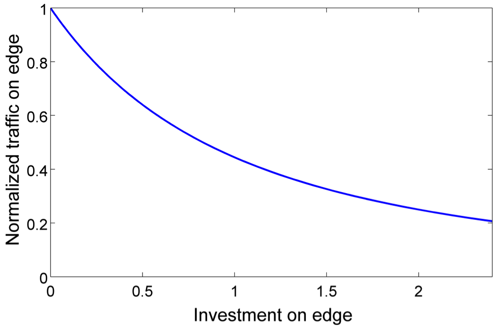
Figure 1: Traffic rate achieved at edge $\left(v_{j},v_{i}\right)$ after an investment on traffic control (in abscissas) is made on that edge.

Using the air transportation network, the parameters, and the cost functions specified above, we solve both the budget-constrained allocation problem using the geometric program in Theorems 3.1. The solution of the budget-constrained allocation problem is summarized in Fig. 2. In the left subplot, we represent the colormap of the adjacency matrix of the air transportation network under study. The color of each pixel in this plot corresponds to the value of $\overline{w}_{ij}$, the maximum achievable traffic in each edge, measured in MPPY. To each one of the 56 airports under study, we have associated a number which corresponds to its ranking with respect to incoming traffic in the airport. In the middle plots of Fig. 2, we represent the incoming traffic (above) and out-going traffic (below) for each one of the airports under consideration.

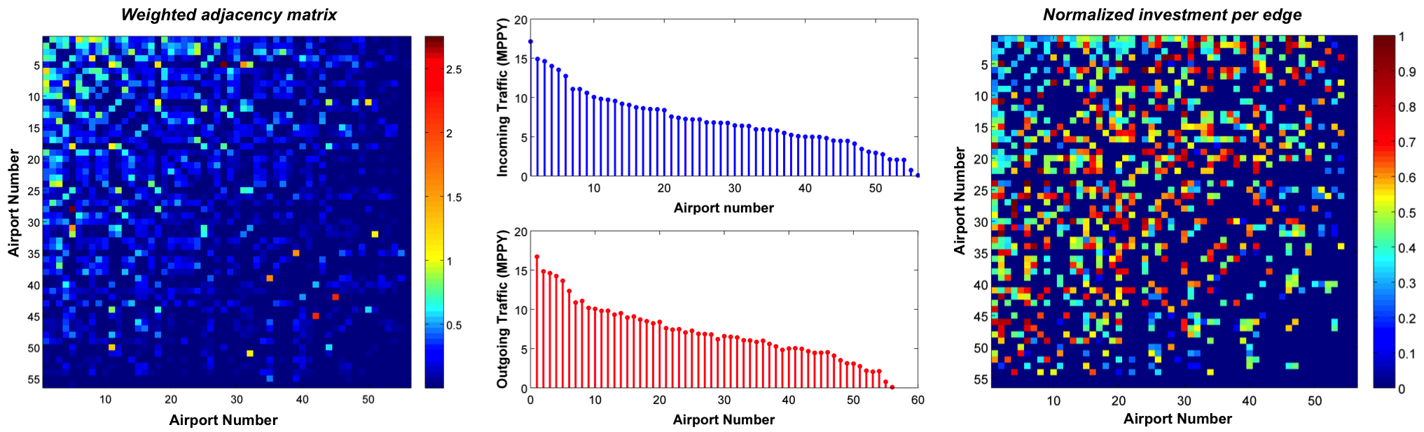
Figure 2: In the left subplot, we represent the colormap of the adjacency matrix of the air transportation network under study. In the middle plots of Fig. 2, we represent the incoming traffic (above) and out-going traffic (below) for each one of the airports under consideration. In the right subplot, we include a colormap corresponding to the optimal allocation of traffic-control resources over the set of directed edges.

Using Theorem 3.1, we solve the budget-constrained allocation problem with a total budget of 300 units. With this budget, we achieve an optimal exponential decay rate of $\varepsilon^{*}=0.021$. The corresponding allocation of traffic-control resources over the set of directed edges is summarized in the right subplot of Fig. 2. The color of the $\left(i,j\right)$ pixel in the colormap represents the amount of control resources invested on edge $\left(v_{j},v_{i}\right)$. A dark blue pixel corresponds to the absence of investment on controlling that edge; thus, the traffic through that edge is not modified and the flow of passengers is equal to $\overline{w}_{ij}$ (the maximum possible flow). A dark red pixel corresponds to a normalized value of investment equal to one. This value corresponds to a saturation of traffic control resources in that edge. In other words, a dark red $\left(i,j\right)$ pixel indicates that the flow of passengers through edge $\left(v_{j},v_{i}\right)$ has been reduced to the minimum possible value, which we have chosen to be $\underline{w}_{ij}=0.2\overline{w}_{ij}$. Notice how, the optimal traffic pattern represented in the right subplot indicates a nontrivial distribution of resources throughout the edges of the transportation network.

The resulting pattern of investment on traffic-control resources is not trivially related with any of the centrality measures popularly considered in the literature. In Fig. 3, we plot the relationship between the amount invested on an edge and a measure of the edge centrality. Although there are some measures of edge centrality in the literature, the concept of node centrality is better developed. We consider in our illustrations two measures of edge centrality based on the centralities of the nodes connected by the edge. In particular, we consider both the eigenvector and the PageRank centralities of the nodes in the network [24]. Denoting by $v_{i}$ and $r_{i}$ the eigenvector and the PageRank centralities of node $v_{i}\in\mathcal{V}$, we define the corresponding eigenvector and PageRank centrality of an edge $\left(v_{j},v_{i}\right)$ as $v_{ij}=v_{i}v_{j}$ and $r_{ij}=r_{i}r_{j}$. In the left and center subplots in Fig. 3, we include two scatter plots where each point represents an edge in the transportation network. The abscissas in those plots are the eigenvector and PageRank centralities of each edge, $v_{ij}$ and $r_{ij}$ respectively, and the ordinates are the amount of traffic-control resources invested on that edge. We observe that there is no trivial law relating the optimal investment on an edge with these edge centrality measurements. For example, we observe in Fig. 3 how some flights connecting airports of low centrality receive higher investment on protection than other flights connecting airports with higher centrality.

Finally, we also included in the right subplot of Fig. 3 a bar plot describing the variation in the achieved rate of containment as a function of the total investment budget. Observe how, for initial values of investment, we achieve a drastic decrease in the containment rate $\lambda_{1}$. This decrease flattens out as we increase the total budget allocated, since the traffic cost function, $h_{ij}$, used in our simulations presents a diminishing marginal benefit on investment. We also observe that the bar diagram becomes completely flat for a level of investment over 900 monetary units. This level corresponds to a saturated level of containments in which all flights have been controlled to have a flow equal to $w_{ij}=\underline{w}_{ij}=0.2\overline{w}_{ij}$.

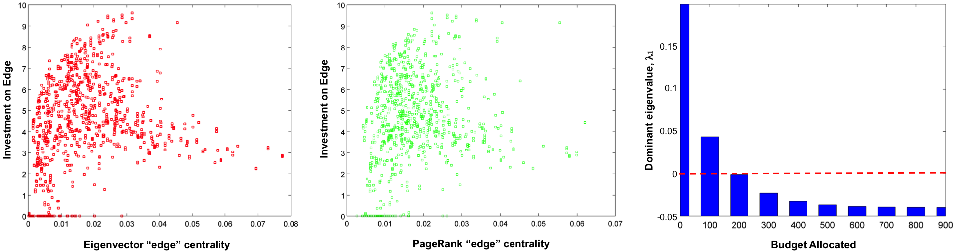
Figure 3: Results from the budget-constrained allocation problem. From left to right, we have (a) a scatter plot with the investment on traffic control versus the eigenvector centrality of each edge, (b) a scatter plot with the investment on traffic control versus the PageRank centrality of each edge, and (c) bar plot describing the variation in the achieved rate of containment as a function of the total investment budget.

5 Conclusions

The problem of allocating protection resources to contain spreading processes has been studied for the case of weighted, directed networks. Relevant applications include the propagation of viruses in computer networks, cascading failures in complex technological networks, and the spreading of epidemics in human populations. Three types of resources has been considered: (i) Traffic control resources which constrain the flow over edges in the contact graph, (ii) preventive resources which ‘immunize’ nodes against the spreading (e.g. vaccines), and (iii) corrective resources which neutralize the infection after it has reached a node (e.g. antidotes). We assume that all resource types have an associated cost (which may vary between nodes or edges). Using the budget-constrained allocation problem, we have found the optimal allocation of resources that contains the spreading process with a fixed budget. Our solution is built on a convex optimization framework, specifically Geometric Programming (GP), which allows us to solve this problem exactly–without relaxations or heuristics–for weighted and directed networks of nonidentical agents in polynomial time. A key feature of the GP approach is that resource allocations of all three types are optimized simultaneously, even in the case where the resource cost functions are heterogeneous throughout the network.

We have demonstrated our optimal protection strategy for the case of a hypothetical world-wide pandemic, spread via the air transportation network. The study has been limited to the airports with the highest passenger traffic worldwide. Given this network, we have computed the optimal resource allocation to protect against such an epidemic. Our simulations indicate nontrivial traffic restriction and resource allocation patterns which cannot, in general, be captured using simple heuristics.

Appendix.

Proof of Lemma 3.2. We define the auxiliary matrix $M\triangleq\mbox{diag}\left(\beta_{i}\right)A-\mbox{diag}\left(\delta_{i}\right)+\Delta I$, where $\Delta\triangleq\max\left\{\delta_{i}\right\}$. Thus, $\lambda_{1}\left(M\right)=\lambda_{1}\left(\mbox{diag}\left(\beta_{i}\right)A-\mbox{diag}\left(\delta_{i}\right)\right)+\Delta$. Notice that both $M$ and $M^{T}$ are nonnegative and irreducible if $\mathcal{G}$ is strongly connected. Hence, from Lemma 3.1, there are two positive vectors $\mathbf{v}$ and $\mathbf{w}$ such that

$$M\mathbf{v} =\rho\mathbf{v},$$

$$\mathbf{w}^{T}M =\rho\mathbf{w}^{T},$$

where $\rho=\rho\left(M\right)=\lambda_{1}\left(M\right)$, and $\mathbf{v}$, $\mathbf{w}$ are the right and left dominant eigenvectors of $M$. From eigenvalue perturbation theory, we have that the increment in the spectral radius of $M$ induced by a matrix increment $\Delta M$ is [25]

$$\rho\left(M+\Delta M\right)-\rho\left(M\right)=\mathbf{w}^{T}\Delta M\mathbf{v}+o\left(\left\|\Delta M\right\|\right).$$ (5.23)

To study the effect of a positive increment in $\beta_{k}$ in the spectral radius, we define $\Delta B=\Delta\beta_{k}\mathbf{e}_{k}\mathbf{e}_{k}^{T}$, for $\Delta\beta_{k}>0$, and apply 5.23 with $\Delta M=\Delta B\,A$. Hence,

$$\rho\left(M+\Delta M\right)-\rho\left(M\right) =\Delta\beta_{k}\mathbf{w}^{T}\mathbf{e}_{k}\mathbf{e}_{k}^{T}A\mathbf{v}+o\left(\left\|\Delta\beta_{k}\right\|\right)$$

$$=\Delta\beta_{k}w_{k}\mathbf{a}_{k}^{T}\mathbf{v}+o\left(\left\|\Delta\beta_{k}\right\|\right)>0,$$

where $\mathbf{a}_{k}^{T}=\mathbf{e}_{k}^{T}A$ and the last inequality if a consequence of $\Delta\beta_{k}$, $w_{k}$, and $\mathbf{a}_{k}^{T}\mathbf{v}$ being all positive. Hence, a positive increment in $\beta_{k}$ induces a positive increment in the spectral radius.

Similarly, to study the effect of a positive increment in $\delta_{k}$ in the spectral radius, we define $\Delta D=\Delta\delta_{k}\mathbf{e}_{k}\mathbf{e}_{k}^{T}$, for $\Delta\delta_{k}>0$. Applying 5.23 with $\Delta M=-\Delta D$, we obtain

$$\rho\left(M+\Delta D\right)-\rho\left(M\right) =-\Delta\delta_{k}\mathbf{w}^{T}\mathbf{e}_{k}\mathbf{e}_{k}^{T}\mathbf{v}+o\left(\left\|\Delta\delta_{k}\right\|\right)$$

$$=-\Delta\delta_{k}w_{k}v_{k}+o\left(\left\|\Delta\delta_{k}\right\|\right)<0.$$

$\blacksquare$

References

- [1] N. Bailey, The mathematical theory of infectious diseases and its applications. Charles Griffin & Company Ltd., 1975.
- [2] M. Garetto, W. Gong, and D. Towsley, “Modeling malware spreading dynamics,” in IEEE INFOCOM 2003, vol. 3, pp. 1869–1879, 2003.
- [3] S. Roy, M. Xue, and S. K. Das, “Security and discoverability of spread dynamics in cyber-physical networks,” IEEE Transactions on Parallel and Distributed Systems, vol. 23, no. 9, pp. 1694–1707, 2012.
- [4] D. J. Watts, R. Muhamad, D. C. Medina, and P. S. Dodds, “Multiscale, resurgent epidemics in a hierarchical metapopulation model,” Proceedings of the National Academy of Sciences, vol. 102, no. 32, pp. 11157–11162, 2005.
- [5] R. Anderson, R. May, and B. Anderson, Infectious Diseases of Humans: Dynamics and Control, vol. 28. Wiley, 1992.
- [6] Y. Wang, D. Chakrabarti, C. Wang, and C. Faloutsos, “Epidemic spreading in real networks: An eigenvalue viewpoint,” in Proc. 22nd Int. Symp. Reliable Distributed Systems, pp. 25–34, 2003.
- [7] A. Ganesh, L. Massoulie, and D. Towsley, “The effect of network topology on the spread of epidemics,” in IEEE INFOCOM 2005, vol. 2, pp. 1455–1466, 2005.
- [8] D. Chakrabarti, Y. Wang, C. Wang, J. Leskovec, and C. Faloutsos, “Epidemic thresholds in real networks,” ACM Transactions on Information and System Security, vol. 10, no. 4, pp. 1–26, 2008.
- [9] P. Van Mieghem, J. Omic, and R. Kooij, “Virus spread in networks,” IEEE/ACM Transactions on Networking, vol. 17, no. 1, pp. 1–14, 2009.
- [10] R. Cohen, S. Havlin, and D. Ben-Avraham, “Efficient immunization strategies for computer networks and populations,” Physical Review Letters, vol. 91, no. 24, p. 247901, 2003.
- [11] C. Borgs, J. Chayes, A. Ganesh, and A. Saberi, “How to distribute antidote to control epidemics,” Random Structures & Algorithms, vol. 37, no. 2, pp. 204–222, 2010.
- [12] F. Chung, P. Horn, and A. Tsiatas, “Distributing antidote using pagerank vectors,” Internet Mathematics, vol. 6, no. 2, pp. 237–254, 2009.
- [13] Y. Wan, S. Roy, and A. Saberi, “Designing spatially heterogeneous strategies for control of virus spread,” Systems Biology, IET, vol. 2, no. 4, pp. 184–201, 2008.
- [14] E. Gourdin, J. Omic, and P. Van Mieghem, “Optimization of network protection against virus spread,” in 8th International Workshop on the Design of Reliable Communication Networks, pp. 86–93, 2011.
- [15] V. M. Preciado, M. Zargham, C. Enyioha, A. Jadbabaie, and G. Pappas, “Optimal vaccine allocation to control epidemic outbreaks in arbitrary networks,” in IEEE Conference on Decision and Control, 2013.
- [16] V. M. Preciado, F. Darabi Sahneh, and C. Scoglio, “A convex framework for optimal investment on disease awareness in social networks,” in IEEE Global Conference on Signal and Information Processing, 2013.
- [17] G. H. Weiss and M. Dishon, “On the asymptotic behavior of the stochastic and deterministic models of an epidemic,” Mathematical Biosciences, vol. 11, no. 3, pp. 261–265, 1971.
- [18] P. V. Mieghem and J. Omic, “In-homogeneous virus spread in networks,” arXiv preprint arXiv:1306.2588, 2013.
- [19] P. Van Mieghem, Performance analysis of communications networks and systems. Cambridge University Press, 2006.
- [20] S. Boyd and L. Vandenberghe, Convex optimization. Cambridge university press, 2004.
- [21] S. Boyd, S.-J. Kim, L. Vandenberghe, and A. Hassibi, “A tutorial on geometric programming,” Optimization and engineering, vol. 8, no. 1, pp. 67–127, 2007.
- [22] C. D. Meyer, Matrix analysis and applied linear algebra. SIAM, 2000.
- [23] C. M. Schneider, T. Mihaljev, S. Havlin, and H. J. Herrmann, “Suppressing epidemics with a limited amount of immunization units,” Physical Review E, vol. 84, no. 6, p. 061911, 2011.
- [24] M. Newman, Networks: An introduction. Cambridge University Press, 2010.
- [25] L. N. Trefethen and D. Bau III, Numerical linear algebra. No. 50, Siam, 1997.