Electromagnetic wave propagation in random waveguides

Abstract

We study long range propagation of electromagnetic waves in random waveguides with rectangular cross-section and perfectly conducting boundaries. The waveguide is filled with an isotropic linear dielectric material, with randomly fluctuating electric permittivity. The fluctuations are weak, but they cause significant cumulative scattering over long distances of propagation of the waves. We decompose the wave field in propagating and evanescent transverse electric and magnetic modes with random amplitudes that encode the cumulative scattering effects. They satisfy a coupled system of stochastic differential equations driven by the random fluctuations of the electric permittivity. We analyze the solution of this system with the diffusion approximation theorem, under the assumption that the fluctuations decorrelate rapidly in the range direction. The result is a detailed characterization of the transport of energy in the waveguide, the loss of coherence of the modes and the depolarization of the waves due to cumulative scattering.

1 Introduction

We study electromagnetic wave propagation in waveguides. There is extensive applied literature on this subject [17, 18, 16, 11, 5, 19] which includes open and closed waveguides, waveguides with losses, boundary corrugation and heterogeneous media. Here we consider the setup illustrated in Figure 1, for a waveguide with rectangular cross-section $\Omega=(0,L_{1})\times(0,L_{2})$, filled with an isotropic linear dielectric material. The waves are trapped by perfectly conducting boundaries and propagate in the range direction $z$. The cross-range coordinates are ${\bf x}=(x_{1},x_{2})\in\Omega$. The main goal of the paper is to analyze long range wave propagation in waveguides with imperfections. We refer to [14, 6, 9, 1, 2] and [7, Chapter 20] for rigorous mathematical studies of long range wave propagation in imperfect acoustic waveguides, and to [4, 3, 8] for their application to imaging and time reversal. Here we extend the theory to electromagnetic waves.

We focus attention on waveguides with imperfections due to a heterogeneous dielectric, but the ideas should extend to waveguides with corrugated boundaries. Such waveguides can be analyzed by changing coordinates to flatten the boundary fluctuations as was done in [1] for sound waves, or by using so-called local normal mode decompositions as proposed in [18, chapter 9]. Our waveguide has straight walls and is filled with a dielectric material that has numerous inhomogeneities (imperfections). These are weak scatterers, so their effect is negligible in the vicinity of the source of the waves. However, the inhomogeneities cause significant cumulative wave scattering over long ranges. To quantify the cumulative scattering effects we study the following questions: How are the modal wave components coupled by scattering? How do the waves depolarize? How do the waves lose coherence? Can we calculate from first principles the scattering mean free paths, which are the range scales over which the modal wave components lose coherence? How is energy transported at long ranges in the waveguides? Can we quantify the equipartition distance where cumulative scattering is so strong that the waves lose all information about the source? How does the equipartition distance compare with the mode dependent scattering mean free paths?

To answer these questions we model the scalar valued electric permittivity $\varepsilon$ of the dielectric as a random process. The random model is motivated by the fact that in applications the imperfections can never be known in detail. They are the uncertain microscale of the medium, the fluctuations of $\varepsilon(\vec{{\bf x}})$ in $\vec{{\bf x}}=({\bf x},z)$, so we model them as random. The fluctuations are small, on a scale (correlation length) comparable to the wavelength. We assume that there is no dissipation in the medium, meaning that $\varepsilon(\vec{{\bf x}})$ is real, positive. Complex valued permittivities $\varepsilon(\omega,\vec{{\bf x}})$ which are typically required by causality i.e., Kramers-Kronig relations, can be incorporated in the model. We do not consider them here for simplicity, and because we are concentrating on the analysis at a single frequency $\omega$. Extensions to multi frequency analysis of wave propagation in dispersive and lossy media can be done, using techniques like in [6, 14, 1] and [7, chapter 20], but we leave them for a different publication.

Fig. 1: Schematic of the setup. The waveguide is unbounded in the range direction $z$ and has rectangular cross-section in the plane $(x_{1},x_{2})$, with sides $L_{1}$ and $L_{2}$.

The paper is organized as follows: We begin in section 2 with the setup. We state Maxwell’s equations and the boundary conditions satisfied by the electromagnetic field. Then we follow the approach in [17] and solve for the components $E_{z}(\omega,\vec{{\bf x}})$ and $H_{z}(\omega,\vec{{\bf x}})$ of the electric and magnetic fields in the range direction. We obtain a $4\times 4$ system of partial differential equations for the components ${\bf E}(\omega,\vec{{\bf x}})$ and ${\bf H}(\omega,\vec{{\bf x}})$ of the fields in the cross-range plane. We analyze in section 3 its solution ${\bf E}_{o}(\omega,\vec{{\bf x}})$ and ${\bf H}_{o}(\omega,\vec{{\bf x}})$ in ideal waveguides with constant permitivity $\varepsilon_{o}$. It is a superposition of uncoupled transverse electric and transverse magnetic modes. The random model of the waveguide is introduced in section 4. Because the amplitude of the fluctuations of $\varepsilon(\vec{{\bf x}})$ is small, of order $\epsilon\ll 1$, the system of equations for ${\bf E}(\omega,\vec{{\bf x}})$ and ${\bf H}(\omega,\vec{{\bf x}})$ is a perturbation of that in ideal waveguides. The remainder of the paper is concerned with the asymptotic analysis of ${\bf E}(\omega,\vec{{\bf x}})$ and ${\bf H}(\omega,\vec{{\bf x}})$ at long ranges, in the limit $\epsilon\to 0$. We consider long ranges because the $\epsilon\to 0$ limit of ${\bf E}(\omega,\vec{{\bf x}})$ and ${\bf H}(\omega,\vec{{\bf x}})$ is the same as the ideal waveguide solution ${\bf E}_{o}(\omega,\vec{{\bf x}})$ and ${\bf H}_{o}(\omega,\vec{{\bf x}})$ when the waves do not propagate far from the source. Our analysis is based on the decomposition of ${\bf E}(\omega,\vec{{\bf x}})$ and ${\bf H}(\omega,\vec{{\bf x}})$ in transverse electric and magnetic modes, with random amplitudes that encode the cumulative scattering effects, as explained in section 5. The long range scaling and the diffusion limit approximation for analyzing the wave field as $\epsilon\to 0$ are stated in section 6. The main results of the paper are in section 7, where we characterize the limit process. Explicitly, we describe the loss of coherence and depolarization of the waves due to cumulative scattering, and the transport of energy. We also show that as we let the range grow, the waves scatter so much that they eventually reach the equipartition regime, where they lose all information about the source. We end with a summary in section 8.

2 Setup

Let $\vec{\bf e}_{1}$, $\vec{\bf e}_{2}$ and $\vec{\bf e}_{z}$ be the unit vectors along the coordinate axes, and use bold letters with an arrow on top for three dimensional vectors, and bold letters for two dimensional vectors in the cross-range plane. Exlicitly, we write

$$\vec{\bf H}={\rm H}_{1}\vec{\bf e}_{1}+{\rm H}_{2}\vec{\bf e}_{2}+{\rm H}_{z}\vec{\bf e}_{z}\,,\qquad{\bf H}=({\rm H}_{1},{\rm H}_{2})\,,$$ (1)

for the magnetic field $\vec{\bf H}(\omega,\vec{{\bf x}})$, and similarly for the electric field $\vec{\bf E}(\omega,\vec{{\bf x}})$ and electric displacement $\vec{\bf D}(\omega,\vec{{\bf x}})$. They satisfy Maxwell’s equations

$$\vec{\nabla}\times\vec{\bf H}(\omega,\vec{{\bf x}}) =\vec{\boldsymbol{\mathcal{J}}}(\omega,\vec{{\bf x}})-i\omega\vec{\bf D}(\omega,\vec{{\bf x}})\,,$$ (2)

$$\vec{\nabla}\times\vec{\bf E}(\omega,\vec{{\bf x}}) =i\omega\mu_{o}\vec{\bf H}(\omega,\vec{{\bf x}})\,,$$ (3)

$$\vec{\nabla}\cdot\vec{\bf H}(\omega,\vec{{\bf x}}) =0\,,$$ (4)

$$\vec{\nabla}\cdot\vec{\bf D}(\omega,\vec{{\bf x}}) =\rho(\omega,\vec{{\bf x}})\,,$$ (5)

where $\vec{\boldsymbol{\mathcal{J}}}$ and $\rho$ are the current source density and free charge density, and $\mu_{o}$ is the magnetic permeability, assumed constant. We denote by

$$\vec{\nabla}=\partial_{x_{1}}\vec{\bf e}_{1}+\partial_{x_{2}}\vec{\bf e}_{2}+\partial_{z}\vec{\bf e}_{z}\,$$

the three dimensional gradient and by $\vec{\nabla}\times$ and $\vec{\nabla}\cdot$ the curl and divergence operators.

The current source density

$$\vec{\boldsymbol{\mathcal{J}}}(\omega,\vec{{\bf x}})=\left({\boldsymbol{\mathcal{J}}}(\omega,\vec{{\bf x}}),\mathcal{J}_{z}(\omega,\vec{{\bf x}})\right)=\left({\bf J}(\omega,{\bf x}),{\rm J}_{z}(\omega,{\bf x})\right)\delta(z)\,,$$ (6)

models a source at the origin of range, supported in the interior of $\Omega$. The Fourier transform $\rho(\omega,\vec{{\bf x}})$ of the free charge density can be obtained from the continuity of charge derived from (2) and (5)

$$-i\omega\rho(\omega,\vec{{\bf x}})+\vec{\nabla}\cdot\vec{\boldsymbol{\mathcal{J}}}(\omega,\vec{{\bf x}})=0\,.$$ (7)

It vanishes at ranges $z\neq 0$.

The electric displacement is proportional to the electric field

$$\vec{\bf D}(\omega,\vec{{\bf x}})=\varepsilon(\vec{{\bf x}})\vec{\bf E}(\omega,\vec{{\bf x}})\,,$$ (8)

with scalar valued, positive and bounded electric permittivity $\varepsilon$. The analysis is for a single frequency, so we simplify the notation by omitting henceforth $\omega$ from the arguments of the fields.

2.1 The $4\times 4$ system of equations

We study the evolution of the two dimensional vectors ${\bf E}(\vec{{\bf x}})$ and ${\bf H}(\vec{{\bf x}})$ for $z>0$. They determine the components $E_{z}(\vec{{\bf x}})$ and $H_{z}(\vec{{\bf x}})$ in the range direction of the electric and magnetic fields, as follows from equations (2)-(3)

$${\rm H}_{z}(\vec{{\bf x}}) =-\frac{i}{\omega\mu_{o}}\nabla^{\perp}\cdot{\bf E}(\vec{{\bf x}})\,,$$ (9)

$${\rm E}_{z}(\vec{{\bf x}}) =\frac{i}{\omega\varepsilon(\vec{{\bf x}})}\left[\nabla^{\perp}\cdot{\bf H}(\vec{{\bf x}})-\mathcal{J}_{z}(\vec{{\bf x}})\right]\,,$$ (10)

with $\nabla^{\perp}=(-\partial_{x_{2}},\partial_{x_{1}})$ the perpendicular gradient in the cross-range plane. The $4\times 4$ system of equations for ${\bf E}(\vec{{\bf x}})$ and ${\bf H}(\vec{{\bf x}})$ is

$$\partial_{z}{\bf E}(\vec{{\bf x}}) =\frac{i}{\omega}\nabla\left[\frac{1}{\varepsilon(\vec{{\bf x}})}\nabla^{\perp}\cdot{\bf H}(\vec{{\bf x}})\right]-\frac{i}{\omega}\nabla\left[\frac{\mathcal{J}_{z}(\vec{{\bf x}})}{\varepsilon(\vec{{\bf x}})}\right]-i\omega\mu_{o}{\bf H}^{\perp}(\vec{{\bf x}})\,,$$ (11)

$$\partial_{z}{\bf H}(\vec{{\bf x}}) =-\frac{i}{\omega\mu_{o}}\nabla\left[\nabla^{\perp}\cdot{\bf E}(\vec{{\bf x}})\right]+i\omega\varepsilon(\vec{{\bf x}}){\bf E}^{\perp}(\vec{{\bf x}})-{\boldsymbol{\mathcal{J}}}^{\perp}(\vec{{\bf x}})\,.$$ (12)

Here $\nabla=(\partial_{x_{1}},\partial_{x_{2}})$ is the gradient in the cross-range plane, and we let ${\bf a}^{\perp}=(-a_{2},a_{1})$ denote the rotation of any vector ${\bf a}=(a_{1},a_{2})$ by $90$ degrees, counter-clockwise.

Note that equations (9)-(12) contain all the information in the Maxwell system (2)-(5). Indeed, (4) follows from (9) and (11)

$$\vec{\nabla}\cdot\vec{\bf H}(\vec{{\bf x}}) =\nabla\cdot{\bf H}(\vec{{\bf x}})+\partial_{z}{\rm H}_{z}(\vec{{\bf x}})$$

$$=\nabla\cdot{\bf H}(\vec{{\bf x}})-\frac{i}{\omega\mu_{o}}\nabla^{\perp}\cdot\partial_{z}{\bf E}(\vec{{\bf x}})$$

$$=\nabla\cdot{\bf H}(\vec{{\bf x}})-\nabla^{\perp}\cdot{\bf H}^{\perp}(\vec{{\bf x}})$$

$$=0\,,$$

because $\nabla^{\perp}\cdot\nabla a(\vec{{\bf x}})=0$ for any twice continuously differentiable function $a(\vec{{\bf x}})$. Similarly, (5) follows from (10) and (12)

$$\vec{\nabla}\cdot\vec{\bf D}(\vec{{\bf x}}) =\nabla\cdot{\bf D}(\vec{{\bf x}})+\partial_{z}{\rm D}_{z}(\vec{{\bf x}})$$

$$=\nabla\cdot\left[\varepsilon(\vec{{\bf x}}){\bf E}(\vec{{\bf x}})\right]+\frac{i}{\omega}\left[\nabla^{\perp}\cdot\partial_{z}{\bf H}(\vec{{\bf x}})-\partial_{z}\mathcal{J}_{z}(\vec{{\bf x}})\right]$$

$$=\nabla\cdot\left[\varepsilon(\vec{{\bf x}}){\bf E}(\vec{{\bf x}})\right]-\nabla^{\perp}\cdot\left[\varepsilon(\vec{{\bf x}}){\bf E}^{\perp}(\vec{{\bf x}})\right]-\frac{i}{\omega}\left[\nabla^{\perp}\cdot{\boldsymbol{\mathcal{J}}}^{\perp}(\vec{{\bf x}})+\partial_{z}\mathcal{J}_{z}(\vec{{\bf x}})\right]$$

$$=-\frac{i}{\omega}\vec{\nabla}\cdot\vec{\boldsymbol{\mathcal{J}}}(\vec{{\bf x}})$$

$$=\rho(\vec{{\bf x}})\,,$$

where we used (8) and the continuity of charge relation (7).

2.2 Boundary conditions

The boundary conditions at the perfectly conducting boundary $\partial\Omega$ are [12, Chapter 8]

$$\vec{\bf n}({\bf x})\times\vec{\bf E}(\vec{{\bf x}})=0\,$$ (13)

for $\vec{{\bf x}}=({\bf x},z)$ and ${\bf x}\in\partial\Omega$. The outer normal $\vec{\bf n}({\bf x})=({\bf n}({\bf x}),0)$ at $\partial\Omega$ is independent of the range and is orthogonal to $\vec{\bf e}_{z}$. Thus, equations (13) say that the tangential components of the electric field vanish at the boundary. Explicitly,

$${\rm E}_{z}(\vec{{\bf x}}) =0\,,\qquad{\bf n}^{\perp}({\bf x})\cdot{\bf E}(\vec{{\bf x}})=0\,.$$ (14)

We need more boundary conditions at $\partial\Omega$ to specify uniquely the solution of (11-12), but they can be derived from Maxwell’s equations (2-3), conditions (14), and our assumptions on the source density (6), as explained in section 3.

The fields are bounded and outgoing at $|z|\to\pm\infty$. We explain in section 4.1 that the causality of the problem in the time domain allows us to restrict the fluctuations of $\varepsilon(\vec{{\bf x}})$ to a finite range interval, and thus justify the outgoing boundary conditions.

2.3 Conservation of energy

The fields ${\bf E}(\vec{{\bf x}})$ and ${\bf H}(\vec{{\bf x}})$ satisfy an energy conservation relation, stated in the following proposition, and used in the analysis in section 7.

Proposition 1.

For any $z>0$, we have the conservation relation

$$\mathcal{S}(z)=-\int_{\Omega}d{\bf x}\,\operatorname{Re}\left[{\bf E}(\vec{{\bf x}})\cdot\overline{{\bf H}^{\perp}(\vec{{\bf x}})}\right]=\mathcal{S}(0+).$$ (15)

where the bar denotes complex conjugate.

Note that

$$\vec{\bf S}(\vec{{\bf x}})=\frac{1}{2}\operatorname{Re}\left[\vec{\bf E}(\vec{{\bf x}})\times\overline{\vec{\bf H}(\vec{{\bf x}})}\right]$$

is the time average of the Poynting vector of a time harmonic wave [12, chapter 7]. Therefore,

$$\mathcal{S}(z)=2\int_{\Omega}d{\bf x}\,\vec{\bf e}_{z}\cdot\vec{\bf S}(\vec{{\bf x}})\,$$

is twice the flux of energy in the range direction, and (15) states that it is conserved for all $z>0$.

To derive (15) we obtain from (2)-(3) that

$$\vec{\nabla}\cdot\left[\vec{\bf E}(\vec{{\bf x}})\times\overline{\vec{\bf H}(\vec{{\bf x}})}\right] =\overline{\vec{\bf H}(\vec{{\bf x}})}\cdot\left[\vec{\nabla}\times\vec{\bf E}(\vec{{\bf x}})\right]-\vec{\bf E}(\vec{{\bf x}})\cdot\left[\vec{\nabla}\times\overline{\vec{\bf H}(\vec{{\bf x}})}\right]$$

$$=i\omega\mu_{o}\left|\vec{\bf H}(\vec{{\bf x}})\right|^{2}-i\omega\varepsilon(\vec{{\bf x}})\left|\vec{\bf E}(\vec{{\bf x}})\right|^{2}-\vec{\bf E}(\vec{{\bf x}})\cdot\overline{\vec{\boldsymbol{\mathcal{J}}}(\vec{{\bf x}})}\,,$$

and from the divergence theorem that

$$\int_{\Omega}d{\bf x}\vec{\nabla}\cdot\left[\vec{\bf E}(\vec{{\bf x}})\times\overline{\vec{\bf H}(\vec{{\bf x}})}\right]= \int_{\partial\Omega}ds({\bf x})\,\vec{\bf n}({\bf x})\cdot\left\{(I-\vec{\bf e}_{z}\vec{\bf e}_{z}^{T})\left[\vec{\bf E}(\vec{{\bf x}})\times\overline{\vec{\bf H}(\vec{{\bf x}})}\right]\right\}+$$

$$\int_{\Omega}d{\bf x}\,\partial_{z}\left\{\vec{\bf e}_{z}\cdot\left[\vec{\bf E}(\vec{{\bf x}})\times\overline{\vec{\bf H}(\vec{{\bf x}})}\right]\right\}\,.$$

The boundary term vanishes because of the boundary conditions (14)

$$\vec{\bf n}({\bf x})\cdot(I-\vec{\bf e}_{z}\vec{\bf e}_{z}^{T})\left[\vec{\bf E}(\vec{{\bf x}})\times\overline{\vec{\bf H}(\vec{{\bf x}})}\right]=E_{z}(\vec{{\bf x}})\,{\bf n}({\bf x})\cdot\overline{{\bf H}^{\perp}(\vec{{\bf x}})}+\overline{H_{z}(\vec{{\bf x}})}\,{\bf n}^{\perp}({\bf x})\cdot{\bf E}(\vec{{\bf x}})=0,$$

and the integrand in the second term satisfies

$$\vec{\bf e}_{z}\cdot\left[\vec{\bf E}(\vec{{\bf x}})\times\overline{\vec{\bf H}(\vec{{\bf x}})}\right]=-{\bf E}(\vec{{\bf x}})\cdot\overline{{\bf H}^{\perp}(\vec{{\bf x}})}\,.$$

The current source density $\overline{\vec{\boldsymbol{\mathcal{J}}}(\vec{{\bf x}})}$ is supported at $z=0$, so we conclude that

$$-\partial_{z}\int_{\Omega}d{\bf x}\,{\bf E}(\vec{{\bf x}})\cdot\overline{{\bf H}^{\perp}(\vec{{\bf x}})}= \int_{\Omega}d{\bf x}\left[i\omega\mu_{o}\left|\vec{\bf H}(\vec{{\bf x}})\right|^{2}-i\omega\varepsilon(\vec{{\bf x}})\left|\vec{\bf E}(\vec{{\bf x}})\right|^{2}\right]\,,\quad z\neq 0\,.$$

The conservation relation (15) follows by taking the real part in this equation.

3 Ideal waveguides

Maxwell’s equations are separable in ideal waveguides with constant permitivity $\varepsilon_{o}$, and it is typical to solve for the longitudinal components $E_{z}(\vec{{\bf x}})$ and $H_{z}(\vec{{\bf x}})$ of the electric and magnetic fields, which then define ${\bf E}(\vec{{\bf x}})$ and ${\bf H}(\vec{{\bf x}})$ [12, chapter8]. The solution is given by a superposition of waves, called modes. They are propagating and evanescent waves and solve Maxwell’s equations with boundary conditions (14). We describe the modes in section 3.1, and then write the solution in section 3.2.

3.1 The waveguide modes

The longitudinal components of the electric and magnetic fields satisfy the boundary conditions

$$E_{z}(\vec{{\bf x}})={\bf n}({\bf x})\cdot\nabla H_{z}(\vec{{\bf x}})=0,\qquad{\bf x}\in\partial\Omega.$$ (16)

The first condition is just (14), and the second follows from Maxwell’s equations (2-3). Indeed, (3) gives

$${\bf H}(\vec{{\bf x}})=\frac{i}{\omega\mu_{o}}\left[\nabla^{\perp}E_{z}(\vec{{\bf x}})-\partial_{z}{\bf E}^{\perp}(\vec{{\bf x}})\right],$$ (17)

so the normal component of ${\bf H}$ at $\partial\Omega$ satisfies

$${\bf n}({\bf x})\cdot{\bf H}(\vec{{\bf x}}) =\frac{i}{\omega\mu_{o}}\left[-{\bf n}^{\perp}({\bf x})\cdot\nabla E_{z}(\vec{{\bf x}})+\partial_{z}{\bf n}^{\perp}({\bf x})\cdot{\bf E}(\vec{{\bf x}})\right]=0,\qquad{\bf x}\in\partial\Omega.$$ (18)

Similarly, we obtain from equation (2) that

$${\bf D}(\vec{{\bf x}})=\frac{i}{\omega}\left[-\nabla^{\perp}H_{z}(\vec{{\bf x}})+\partial_{z}{\bf H}^{\perp}(\vec{{\bf x}})\right],$$ (19)

and the boundary condition (14) implies that

$${\bf n}^{\perp}({\bf x})\cdot{\bf D}(\vec{{\bf x}})=\frac{i}{\omega}\left[-{\bf n}({\bf x})\cdot\nabla H_{z}(\vec{{\bf x}})+\partial_{z}{\bf n}({\bf x})\cdot{\bf H}(\vec{{\bf x}})\right]=0.$$

The Neumann boundary condition (16) on $H_{z}$ follows from this equation and (18).

The waveguide modes are solutions of Maxwell’s equations that depend on the range $z$ as $\exp(\pm i\beta z)$, with mode wavenumber $\beta$ to be defined. We write them as

$$\widetilde{{\bf D}}({\bf x};\pm\beta)e^{\pm i\beta z},\qquad\widetilde{\bf H}({\bf x};\pm\beta)e^{\pm i\beta z},$$ (20)

and similar for the longitudinal components, which satisfy

$$\Delta\widetilde{E}_{z}({\bf x};\pm\beta)+(k^{2}-\beta^{2})\widetilde{E}_{z}({\bf x};\pm\beta) =0,$$ (21)

$$\Delta\widetilde{H}_{z}({\bf x};\pm\beta)+(k^{2}-\beta^{2})\widetilde{H}_{z}({\bf x};\pm\beta) =0,\qquad{\bf x}\in\Omega.$$ (22)

Here $\Delta$ is the Laplacian in ${\bf x}$, $k=\omega/c_{o}$ is the wavenumber and $c_{o}=1/\sqrt{\varepsilon_{o}\nu_{o}}$ is the wave speed.

3.1.1 Spectral decomposition of the Laplacian

The Laplacian operator acting on functions with homogeneous Dirichlet conditions is symmetric negative definite, with countable eigenvalues

$$\lambda_{j}=\left(\frac{\pi j_{1}}{L_{1}}\right)^{2}+\left(\frac{\pi j_{2}}{L_{2}}\right)^{2}\,,$$ (23)

and eigenfunctions

$$\widetilde{E}_{j,z}({\bf x})=\sin\left(\frac{\pi j_{1}x_{1}}{L_{1}}\right)\sin\left(\frac{\pi j_{2}x_{2}}{L_{2}}\right).$$ (24)

The indexes $j_{1}$ and $j_{2}$ are natural numbers satisfying the constraint $j_{1}^{2}+j_{2}^{2}\neq 0$. We associate the pair $(j_{1},j_{2})$ to the index $j$ because $\mathbb{N}\times\mathbb{N}$ is countable, and enumerate the eigenvalues in increasing order.

Similarly, the Laplacian operator acting on functions with homogeneous Neumann conditions is symmetric negative semidefinite, with the same eigenvalues as (23), and eigenfunctions

$$\widetilde{H}_{j,z}({\bf x})=\cos\left(\frac{\pi j_{1}x_{1}}{L_{1}}\right)\cos\left(\frac{\pi j_{2}x_{2}}{L_{2}}\right).$$ (25)

Thus, we see that the electric and magnetic fields have the same mode wavenumbers $\beta$, which take the discrete values $\sqrt{k^{2}-\lambda_{j}}$. We write them as

$$\beta=\left\{\begin{array}[]{ll}\beta_{j},&j=1,\ldots,N,\\ i\beta_{j},&j>N,\end{array}\right.\qquad{\rm for}~{}~{}\beta_{j}=\sqrt{|k^{2}-\lambda_{j}|},$$ (26)

to emphasize that only the first $N$ are real. The infinitely many modes that correspond to eigenvalues $\lambda_{j}>k^{2}$ are evanescent. We assume that $\beta_{N}\neq 0$, so there are no standing waves in the waveguide.

3.1.2 The transverse electric and magnetic modes

It follows immediately from (17), (19), (24) and (25) that $\widetilde{\bf D}$ and $(\widetilde{\bf H})^{\perp}$ are given by superpositions of the vectors $\nabla^{\perp}\widetilde{H}_{j,z}({\bf x})$ and $\nabla\widetilde{E}_{j,z}({\bf x})$. Thus, we define the vectors

$${\boldsymbol{\varphi}}_{j}^{(1)}=\alpha_{j}\nabla^{\perp}\widetilde{H}_{j,z}({\bf x})=\alpha_{j}\left(\begin{matrix}\frac{\pi j_{2}}{L_{2}}\cos\left(\frac{\pi j_{1}x_{1}}{L_{1}}\right)\sin\left(\frac{\pi j_{2}x_{2}}{L_{2}}\right)\\ \\ -\frac{\pi j_{1}}{L_{1}}\sin\left(\frac{\pi j_{1}x_{1}}{L_{1}}\right)\cos\left(\frac{\pi j_{2}x_{2}}{L_{2}}\right)\end{matrix}\right)\,,$$ (27)

and

$${\boldsymbol{\varphi}}_{j}^{(2)}=\alpha_{j}\nabla\widetilde{E}_{j,z}({\bf x})=\alpha_{j}\left(\begin{matrix}\frac{\pi j_{1}}{L_{1}}\cos\left(\frac{\pi j_{1}x_{1}}{L_{1}}\right)\sin\left(\frac{\pi j_{2}x_{2}}{L_{2}}\right)\\ \\ \frac{\pi j_{2}}{L_{2}}\sin\left(\frac{\pi j_{1}x_{1}}{L_{1}}\right)\cos\left(\frac{\pi j_{2}x_{2}}{L_{2}}\right)\end{matrix}\right)\,,$$ (28)

normalized by

$$\alpha_{j}=\left\{\begin{array}[]{ll}\frac{2}{\sqrt{\lambda_{j}L_{1}L_{2}}},&j=(j_{1},j_{2}),\quad j_{1}j_{2}\neq 0,\\ \\ \sqrt{\frac{2}{\lambda_{j}L_{1}L_{2}}},&j=(j_{1},j_{2}),\quad j_{1}j_{2}=0.\end{array}\right.$$ (29)

so that

$$\|{\boldsymbol{\varphi}}^{(s)}_{j}\|^{2}=\int_{\Omega}d{\bf x}\left|{\boldsymbol{\varphi}}_{j}^{(s)}({\bf x})\right|^{2}=1,\qquad s=1,2.$$

The vectors indexed by $s=1$ correspond to transverse electric (TE) modes. Indeed, they satisfy

$$\nabla\cdot{\boldsymbol{\varphi}}^{(1)}({\bf x})=0,\qquad{\bf x}\in\Omega,$$ (30)

so when we set ${\bf H}^{\perp}(\vec{{\bf x}})={\boldsymbol{\varphi}}^{(1)}({\bf x})e^{i\beta_{j}z}$ in (10) we get $E_{z}(\vec{{\bf x}})=0$. Similarly, the vectors indexed by $s=2$ correspond to transverse magnetic (TM) modes. They satisfy

$$\nabla^{\perp}\cdot{\boldsymbol{\varphi}}^{(2)}({\bf x})=0,\qquad{\bf x}\in\Omega,$$ (31)

and give $H_{z}(\vec{{\bf x}})=0$ by equation (9).

The superposition of ${\boldsymbol{\varphi}}_{j}^{(1)}({\bf x})$ and ${\boldsymbol{\varphi}}_{j}^{(2)}({\bf x})$ in the definition of the fields $\widetilde{\bf E}$ and $(\widetilde{\bf H})^{\perp}$ is their Helmholtz decomposition in a divergence free part and a curl free part.

3.1.3 Analogous derivation of the waveguide modes

We could have arrived at the same wave decomposition if we worked directly with the transverse components ${\bf D}$ and ${\bf H}$ of the fields. This observation is relevant because when the permittivity varies in $\vec{{\bf x}}$, as in the random waveguide, it is no longer possible to solve independently for the longitudinal wave fields $E_{z}$ and $D_{z}$.

We let

$${\bf H}(\vec{{\bf x}})=c_{o}{\bf U}^{\perp}(\vec{{\bf x}}),$$ (32)

where ${\bf U}$ is the rotated magnetic field scaled by $1/c_{o}$. It is convenient to work in the ${\bf D}$ and ${\bf U}$ variables because as we see below, they satisfy the same boundary conditions and have the same physical units. Note from (27) and (28) that ${\boldsymbol{\varphi}}^{(s)}({\bf x})$ are eigenfunctions of the vector Laplacian

$$\Delta{\boldsymbol{\varphi}}_{j}^{(s)}({\bf x})=\nabla\left[\nabla\cdot{\boldsymbol{\varphi}}_{j}^{(s)}({\bf x})\right]+\nabla^{\perp}\left[\nabla^{\perp}\cdot{\boldsymbol{\varphi}}_{j}^{(s)}({\bf x})\right]=-\lambda_{j}{\boldsymbol{\varphi}}_{j}^{(s)}({\bf x}),$$ (33)

for ${\bf x}\in\Omega$, with boundary conditions

$${\bf n}^{\perp}({\bf x})\cdot{\boldsymbol{\varphi}}_{j}^{(s)}({\bf x})=0,\qquad\nabla\cdot{\boldsymbol{\varphi}}_{j}^{(s)}({\bf x})=0,\qquad{\bf x}\in\partial\Omega.$$ (34)

The index $s=1,2$ corresponds to the multiplicity $\mathfrak{M}_{j}$ of the eigenvalues. We can limit the multiplicity of $\lambda_{j}$ by assuming that the waveguide dimensions satisfy $L_{1}/L_{2}\neq\mathbb{Q}$. This implies that

$$\lambda_{j}\neq\lambda_{j^{\prime}}\,,\qquad{\rm if}~{}~{}j=(j_{1},j_{2})\neq j^{\prime}=(j_{1}^{\prime},j_{2}^{\prime})\,.$$ (35)

When $j=(j_{1},j_{2})$ and either $j_{1}$ or $j_{2}$ are zero, $\mathfrak{M}_{j}=1$, and only the TE modes ${\boldsymbol{\varphi}}_{j}^{(1)}({\bf x})$ exist. Otherwise $\mathfrak{M}_{j}=2$.

The eigenfunctions satisfy the orthogonality relations

$$\left<{\boldsymbol{\varphi}}_{j}^{(s)}\,,{\boldsymbol{\varphi}}_{j^{\prime}}^{(s^{\prime})}\right>=\int_{\Omega}d{\bf x}\,{\boldsymbol{\varphi}}_{j}^{(s)}({\bf x})\cdot{\boldsymbol{\varphi}}_{j^{\prime}}^{(s^{\prime})}({\bf x})=\delta_{jj^{\prime}}\delta_{ss^{\prime}}\,.$$ (36)

and $\left\{{\boldsymbol{\varphi}}_{j}^{(s)}\right\}_{1\leq s\leq\mathfrak{M}_{j},j\geq 1}$ is a complete set that can be used to describe an arbitrary electromagnetic wave field in the waveguide [12, chapter8].

The boundary conditions (34) are consistent with the conditions satisfied by ${\bf D}(\vec{{\bf x}})$ and ${\bf U}(\vec{{\bf x}})$, derived from Maxwell’s equations. Indeed, equations (10), (14) and the assumption (6) on the source density give that

$$\nabla\cdot{\bf U}(\vec{{\bf x}})=-\frac{1}{c_{o}}\nabla^{\perp}\cdot{\bf H}(\vec{{\bf x}})=0,\qquad{\bf x}\in\partial\Omega.$$ (37)

Moreover, equation (18) says that

$${\bf n}^{\perp}({\bf x})\cdot{\bf U}(\vec{{\bf x}})=-\frac{1}{c_{o}}{\bf n}({\bf x})\cdot{\bf H}(\vec{{\bf x}})=0,\qquad{\bf x}\in\partial\Omega.$$ (38)

For the electric displacement we already know from (14) that

$${\bf n}^{\perp}({\bf x})\cdot{\bf D}(\vec{{\bf x}})=0,\qquad{\bf x}\in\partial\Omega.$$ (39)

The divergence condition follows from (19) and (37)

$$\nabla\cdot{\bf D}(\vec{{\bf x}})=0,\qquad{\bf x}\in\partial\Omega,$$ (40)

and since $\partial_{z}D_{z}=0$, it is consistent with the conservation of charge.

3.2 The solution in ideal waveguides

We expand ${\bf D}(\vec{{\bf x}})$ and ${\bf U}(\vec{{\bf x}})$ in the basis $\left\{{\boldsymbol{\varphi}}_{j}^{(s)}\right\}_{1\leq s\leq\mathfrak{M}_{j},j\geq 1}$ and associate to each ${\boldsymbol{\varphi}}_{j}^{(s)}(x)$ a mode, which is a propagating or evanescent wave. We rename the fields ${\bf D}_{o}(\vec{{\bf x}})$ and ${\bf U}_{o}(\vec{{\bf x}})$ to remind us that we are in the ideal waveguide.

Using the identities

$$k^{2}{\boldsymbol{\varphi}}_{j}^{(s)}({\bf x})+\nabla\left[\nabla\cdot{\boldsymbol{\varphi}}_{j}^{(s)}(\vec{{\bf x}})\right] =\left[k^{2}\delta_{s1}+(k^{2}-\lambda_{j})\delta_{s2}\right]{\boldsymbol{\varphi}}_{j}^{(s)}({\bf x})\,,$$ (41)

$$k^{2}{\boldsymbol{\varphi}}_{j}^{(s)}({\bf x})+\nabla^{\perp}\left[\nabla^{\perp}\cdot{\boldsymbol{\varphi}}_{j}^{(s)}(\vec{{\bf x}})\right] =\left[(k^{2}-\lambda_{j})\delta_{s1}+k^{2}\delta_{s2}\right]{\boldsymbol{\varphi}}_{j}^{(s)}({\bf x})\,,$$ (42)

we obtain that

$${\bf D}_{o}(\vec{{\bf x}})= \sum_{j=1}^{N}\sum_{s=1}^{\mathfrak{M}_{j}}{\boldsymbol{\varphi}}_{j}^{(s)}({\bf x})\left(\sqrt{\frac{k}{\beta_{j}}}\delta_{s1}+\sqrt{\frac{\beta_{j}}{k}}\delta_{s2}\right)\left(A_{j,o}^{\pm(s)}e^{i\beta_{j}z}+B_{j,o}^{\pm(s)}e^{-i\beta_{j}z}\right)+$$

$$\sum_{j>N}\sum_{s=1}^{\mathfrak{M}_{j}}{\boldsymbol{\varphi}}_{j}^{(s)}({\bf x})\left(\sqrt{\frac{k}{\beta_{j}}}\delta_{s1}+\sqrt{\frac{\beta_{j}}{k}}\delta_{s2}\right)\mathfrak{E}_{j,o}^{\pm(s)}e^{-\beta_{j}|z|}\,,\qquad$$ (43)

and

$${\bf U}_{o}(\vec{{\bf x}})= \sum_{j=1}^{N}\sum_{s=1}^{\mathfrak{M}_{j}}{\boldsymbol{\varphi}}_{j}^{(s)}({\bf x})\left(\sqrt{\frac{\beta_{j}}{k}}\delta_{s1}+\sqrt{\frac{k}{\beta_{j}}}\delta_{s2}\right)\left(A_{j,o}^{\pm(s)}e^{i\beta_{j}z}-B_{j,o}^{\pm(s)}e^{-i\beta_{j}z}\right)\pm$$

$$i\sum_{j>N}\sum_{s=1}^{\mathfrak{M}_{j}}{\boldsymbol{\varphi}}_{j}^{(s)}({\bf x})\left(\sqrt{\frac{\beta_{j}}{k}}\delta_{s1}-\sqrt{\frac{k}{\beta_{j}}}\delta_{s2}\right)\mathfrak{E}_{j,o}^{\pm(s)}e^{-\beta_{j}|z|}\,,$$ (44)

for $z\neq 0$. The normalization coefficients $\sqrt{k/\beta_{j}}$ and $\sqrt{\beta_{j}/k}$ are not important here, and could be absorbed in the mode amplitudes. We use them for consistency with the mode expansions for the random waveguide in section 5. There the normalization symmetrizes the system of equations satisfied by the mode amplitudes.

The amplitudes in (43-44) are constant on each side of the source, and are determined by the source density and the outgoing boundary conditions. There are no backward going modes to the right of the source, at positive ranges, so we can set $B_{j,o}^{+(s)}=0$. Similarly, we let $A_{j,o}^{-(s)}=0$. The remaining amplitudes are obtained from the source conditions

$${\bf D}_{o}({\bf x},0+)-{\bf D}_{o}({\bf x},0-) =-\frac{i}{c_{o}k}\nabla{\rm J}_{z}({\bf x})\,,$$

$${\bf U}_{o}({\bf x},0+)-{\bf U}_{o}({\bf x},0-) =-\frac{1}{c_{o}}{\bf J}({\bf x})\,.$$

Substituting (43-44) in these conditions and using the orthogonality relations (36), we get

$$A_{j,o}^{+(s)}= -\frac{1}{2c_{o}}\left(\sqrt{\frac{k}{\beta_{j}}}\delta_{s1}+\sqrt{\frac{\beta_{j}}{k}}\delta_{s2}\right)\left<{\boldsymbol{\varphi}}_{j}^{(s)}\,,{\bf J}\right>-$$

$$\frac{i}{2c_{o}k}\left(\sqrt{\frac{\beta_{j}}{k}}\delta_{s1}+\sqrt{\frac{k}{\beta_{j}}}\delta_{s2}\right)\left<\nabla{\rm J}_{z},{\boldsymbol{\varphi}}_{j}^{(s)}\right>\,,$$ (45)

and

$$B_{j,o}^{-(s)}= -\frac{1}{2c_{o}}\left(\sqrt{\frac{k}{\beta_{j}}}\delta_{s1}+\sqrt{\frac{\beta_{j}}{k}}\delta_{s2}\right)\left<{\boldsymbol{\varphi}}_{j}^{(s)}\,,{\bf J}\right>+$$

$$\frac{i}{2c_{o}k}\left(\sqrt{\frac{\beta_{j}}{k}}\delta_{s1}+\sqrt{\frac{k}{\beta_{j}}}\delta_{s2}\right)\left<\nabla{\rm J}_{z},{\boldsymbol{\varphi}}_{j}^{(s)}\right>\,,$$ (46)

for the propagating modes and

$$\mathfrak{E}_{j,o}^{\pm(s)}= \frac{i}{2c_{o}}\left(\sqrt{\frac{k}{\beta_{j}}}\delta_{s1}-\sqrt{\frac{\beta_{j}}{k}}\delta_{s2}\right)\left<{\boldsymbol{\varphi}}_{j}^{(s)}\,,{\bf J}\right>\mp$$

$$\frac{i}{2c_{o}k}\left(\sqrt{\frac{\beta_{j}}{k}}\delta_{s1}+\sqrt{\frac{k}{\beta_{j}}}\delta_{s2}\right)\left<\nabla{\rm J}_{z},{\boldsymbol{\varphi}}_{j}^{(s)}\right>\,,$$ (47)

for the evanescent modes.

3.2.1 Energy conservation

The energy conservation is obvious in this case, because the amplitudes are constant. Substituting (43-44) in the expression of the flux $\mathcal{S}(z)$ and using the orthogonality relations (36), we obtain that

$$\mathcal{S}(z)=\frac{c_{o}}{\varepsilon_{o}}\int_{\Omega}\operatorname{Re}\left[{\bf D}_{o}(\vec{{\bf x}})\cdot\overline{{\bf U}_{o}(\vec{{\bf x}})}\right]=\sum_{j=1}^{N}\sum_{s=1}^{\mathfrak{M}_{j}}\left(\left|A_{j,o}^{\pm(s)}\right|^{2}-\left|B_{j,o}^{\pm(s)}\right|^{2}\right)\,,\quad\forall z\in\mathbb{R}\,.$$ (48)

The flux changes value at $z=0$, where the source lies, but it is constant for $z\neq 0$,

$$\mathcal{S}(|z|)=\frac{c_{o}}{\varepsilon_{o}}\sum_{j=1}^{N}\sum_{s=1}^{\mathfrak{M}_{j}}\left|A_{j,o}^{+(s)}\right|^{2}=-\mathcal{S}(-|z|)=\frac{c_{o}}{\varepsilon_{o}}\sum_{j=1}^{N}\sum_{s=1}^{\mathfrak{M}_{j}}\left|B_{j,o}^{-(s)}\right|^{2}\,,\qquad z\neq 0\,.$$ (49)

The evanescent modes play no role in the transport of energy.

4 Statement of the problem in the random waveguide

We begin with the model of the small fluctuations. Then we write the perturbed system of equations for the wave fields, which we analyze in the remainder of the paper.

4.1 Model of the fluctuations

Let us denote by $n(\vec{{\bf x}})$ the index of refraction

$$n(\vec{{\bf x}})=\frac{c_{o}}{c(\vec{{\bf x}})}=\sqrt{\frac{\varepsilon(\vec{{\bf x}})}{\varepsilon_{o}}}\,.$$ (50)

It is the ratio of the electromagnetic wave speeds $c_{o}$ and $c(\vec{{\bf x}})=1/\sqrt{\varepsilon(\vec{{\bf x}})\mu_{o}}$ in the homogeneous and heterogeneous medium, respectively. We model the electrical permittivity by

$$\varepsilon(\vec{{\bf x}})=\varepsilon_{o}n^{2}(\vec{{\bf x}})\,,\qquad n^{2}(\vec{{\bf x}})=\left[1+\epsilon\nu(\vec{{\bf x}})\right]1_{(0+,z_{\rm max})}(z)\,,$$ (51)

where $\nu(\vec{{\bf x}})$ is a dimensionless random function assumed twice continuously differentiable, with almost sure bounded derivatives. It has zero mean

$${\mathbb{E}}\left[\nu(\vec{{\bf x}})\right]=0\,,$$ (52)

and it is stationary and mixing in $z$. We refer to [15, Section 4.6.2] for a precise statement of the mixing condition. It means in particular that the covariance

$$\mathcal{R}_{\nu}({\bf x},{\bf x}^{\prime},z)={\mathbb{E}}\left[\nu({\bf x},z)\nu({\bf x}^{\prime},0)\right]$$ (53)

is integrable in $z$. The amplitude of the fluctuations in (51) is scaled by $\epsilon\ll 1$, the small parameter in our asymptotic analysis.

The indicator function $1_{(0+,z_{\rm max})}(z)$ in (51) limits the support of the fluctuations to the range interval $z\in(0+,z_{\rm max})$, where $0+$ denotes a range that is close to zero, but strictly larger than it. The bounded support of the fluctuations is needed to state the outgoing boundary conditions on the electromagnetic wave fields, and may be justified in practice by the causality of the problem in the time domain. During a finite observation time $t_{\rm max}$, the waves are influenced by the medium up to a finite range $z_{\rm max}\approx c_{o}t_{\rm max}\,,$ so we may truncate the fluctuations beyond the range $z_{\rm max}$. That there are no fluctuations at negative ranges may be motivated by two facts: First, the source is at $z=0$ and we wish to study the waves at positive ranges. Second, we will consider a regime where the backscattered field is negligible. Thus, we may neglect at $z>0$ the waves that come from $z<0$, and truncate the fluctuations at $z=0+$.

4.2 The perturbed system of equations in the random waveguide

We work with the electric displacement ${\bf D}(\vec{{\bf x}})$ and the scaled rotated magnetic field ${\bf U}(\vec{{\bf x}})$, defined in equation (32). As we explained in the previous section, this is convenient because the fields satisfy the same boundary conditions and have the same units.

The equations for ${\bf D}(\vec{{\bf x}})$ and ${\bf U}(\vec{{\bf x}})$ follow from (8), (11-12), (51) and (32). We have

$$\partial_{z}{\bf D}(\vec{{\bf x}})= \frac{i}{k}\left\{k^{2}n^{2}(\vec{{\bf x}}){\bf U}(\vec{{\bf x}})+\nabla\left[\nabla\cdot{\bf U}(\vec{{\bf x}})\right]-n^{-2}(\vec{{\bf x}})\nabla n^{2}(\vec{{\bf x}})\nabla\cdot{\bf U}(\vec{{\bf x}})\right\}+$$

$$n^{-2}(\vec{{\bf x}})\partial_{z}n^{2}(\vec{{\bf x}})\,{\bf D}(\vec{{\bf x}})-\frac{i}{c_{o}k}\nabla\mathcal{J}_{z}(\vec{{\bf x}})\,,$$ (54)

for the electric displacement and

$$\partial_{z}{\bf U}(\vec{{\bf x}})= \frac{i}{k}\left\{k^{2}{\bf D}(\vec{{\bf x}})+\nabla^{\perp}\left[\nabla^{\perp}\cdot\left(n^{-2}(\vec{{\bf x}}){\bf D}(\vec{{\bf x}})\right)\right]\right\}-\frac{1}{c_{o}}{\boldsymbol{\mathcal{J}}}(\vec{{\bf x}})\,,$$ (55)

for the rotated magnetic field, where we used that the fluctuations are supported away from the source. Morever, substituting the model (51) of the fluctuations, we obtain

$$\partial_{z}{\bf D}(\vec{{\bf x}})= \frac{i}{k}\left\{k^{2}{\bf U}(\vec{{\bf x}})+\nabla\left[\nabla\cdot{\bf U}(\vec{{\bf x}})\right]\right\}-\frac{i}{c_{o}k}\nabla\mathcal{J}_{z}(\vec{{\bf x}})+$$

$$\epsilon\left\{\partial_{z}\nu(\vec{{\bf x}})\,{\bf D}(\vec{{\bf x}})+\frac{i}{k}\left[k^{2}\nu(\vec{{\bf x}}){\bf U}(\vec{{\bf x}})-\nabla\nu(\vec{{\bf x}})\,\nabla\cdot{\bf U}(\vec{{\bf x}})\right]\right\}+$$

$$\frac{\epsilon^{2}}{2}\left[-\partial_{z}\nu^{2}(\vec{{\bf x}})\,{\bf D}(\vec{{\bf x}})+\frac{i}{k}\nabla\nu^{2}(\vec{{\bf x}})\nabla\cdot{\bf U}(\vec{{\bf x}})\right]+O(\epsilon^{3})\,,$$ (56)

and

$$\partial_{z}{\bf U}(\vec{{\bf x}})= \frac{i}{k}\left\{k^{2}{\bf D}(\vec{{\bf x}})+\nabla^{\perp}\left[\nabla^{\perp}\cdot{\bf D}(\vec{{\bf x}})\right]\right\}-\frac{1}{c_{o}}{\boldsymbol{\mathcal{J}}}(\vec{{\bf x}})-$$

$$\epsilon\frac{i}{k}\left\{\nabla^{\perp}\left[\nu(\vec{{\bf x}})\nabla^{\perp}\cdot{\bf D}(\vec{{\bf x}})\right]+\nabla^{\perp}\left[{\bf D}(\vec{{\bf x}})\cdot\nabla^{\perp}\nu(\vec{{\bf x}})\right]\right\}+$$

$$\epsilon^{2}\frac{i}{k}\left\{\nabla^{\perp}\left[\nu^{2}(\vec{{\bf x}})\nabla^{\perp}\cdot{\bf D}(\vec{{\bf x}})\right]+\nabla^{\perp}\left[{\bf D}(\vec{{\bf x}})\cdot\nabla^{\perp}\nu^{2}(\vec{{\bf x}})\right]\right\}+O(\epsilon^{3})\,,$$ (57)

with remainder involving powers $(\epsilon\nu)^{q}$, for $q\geq 3$. It is of order $\epsilon^{3}$ because $\nu(\vec{{\bf x}})$ is twice differentiable, with almost sure bounded derivatives.

The leading order terms in (56-57) involve the operators (41-42), so we have a perturbation of the problem in the ideal waveguide. The conservation of the energy flux follows from (15) and definitions (8),(51) and (32)

$$\mathcal{S}(z) =\frac{c_{o}}{\varepsilon_{o}}\int_{\Omega}d{\bf x}\,\operatorname{Re}\left[n^{-2}(\vec{{\bf x}})\,{\bf D}(\vec{{\bf x}})\cdot\overline{{\bf U}(\vec{{\bf x}})}\right]$$

$$=\frac{c_{o}}{\varepsilon_{o}}\int_{\Omega}d{\bf x}\,\left[1-\epsilon\nu(\vec{{\bf x}})+\epsilon^{2}\nu^{2}(\vec{{\bf x}})+O(\epsilon^{3})\right]\operatorname{Re}\left[{\bf D}(\vec{{\bf x}})\cdot\overline{{\bf U}(\vec{{\bf x}})}\right]$$

$$=\mathcal{S}(0+)\,,\qquad z>0.$$ (58)

5 Mode decomposition and coupling in random waveguides

The equations in the random waveguide are no longer separable, but $\{{\boldsymbol{\varphi}}_{j}^{(s)}({\bf x})\}_{1\leq s\leq\mathfrak{M}_{j},j\geq 1}$ is an orthonormal basis, so we can still use it to decompose the wave fields for any range $z$. The essential difference in the decomposition is that while the mode amplitudes are constant in ideal waveguides, they vary in range in the random waveguides, due to scattering. The range evolution of the mode amplitudes is described by a coupled system of infinitely many stochastic ordinary differential equations. We show in section 5.3 that we can solve for the amplitudes of the evanescent modes, and thus obtain in section 5.4 a closed and finite system of equations for the amplitudes of the propagating modes. This system is the main result of the section. We use it in section 6 to obtain an explicit long range characterization of the statistical distribution of the electromagnetic wave field.

5.1 Mode decomposition

We decompose the fields as

$${\bf D}(\vec{{\bf x}})= \sum_{j=1}^{N}\sum_{s=1}^{\mathfrak{M}_{j}}{\boldsymbol{\varphi}}_{j}^{(s)}({\bf x})\left(\sqrt{\frac{k}{\beta_{j}}}\delta_{s1}+\sqrt{\frac{\beta_{j}}{k}}\delta_{s2}\right)\left(A_{j}^{(s)}(z)e^{i\beta_{j}z}+B_{j}^{(s)}(z)e^{-i\beta_{j}z}\right)+$$

$$\sum_{j>N}\sum_{s=1}^{\mathfrak{M}_{j}}{\boldsymbol{\varphi}}_{j}^{(s)}({\bf x})\left(\sqrt{\frac{k}{\beta_{j}}}\delta_{s1}+\sqrt{\frac{\beta_{j}}{k}}\delta_{s2}\right)V_{j}^{(s)}(z)\,,\qquad$$ (59)

and

$${\bf U}(\vec{{\bf x}})= \sum_{j=1}^{N}\sum_{s=1}^{\mathfrak{M}_{j}}{\boldsymbol{\varphi}}_{j}^{(s)}({\bf x})\left(\sqrt{\frac{\beta_{j}}{k}}\delta_{s1}+\sqrt{\frac{k}{\beta_{j}}}\delta_{s2}\right)\left(A_{j}^{(s)}(z)e^{i\beta_{j}z}-B_{j}^{(s)}(z)e^{-i\beta_{j}z}\right)\pm$$

$$i\sum_{j>N}\sum_{s=1}^{\mathfrak{M}_{j}}{\boldsymbol{\varphi}}_{j}^{(s)}({\bf x})\left(\sqrt{\frac{\beta_{j}}{k}}\delta_{s1}-\sqrt{\frac{k}{\beta_{j}}}\delta_{s2}\right)v_{j}^{(s)}(z)\,,$$ (60)

for $z\neq 0$. The decomposition is similar to that in ideal waveguides, but the mode amplitudes vary in $z$ due to scattering in the random medium. We show in section (5.2) that the forward and backward going mode amplitudes $A_{j}^{(s)}$ and $B_{j}^{(s)}$ are coupled with each other and with the evanescent modes written in (59-60) as $V_{j}^{(s)}(z)$ and $v_{j}^{(s)}(z)$. In ideal waveguides the evanescent modes were equal to $\mathfrak{E}_{j,o}^{(s)}{\rm exp}(-\beta_{j}z)$, for $1\leq s\leq\mathfrak{M}_{j}$ and $j>N$. They have a more complicated expression in random waveguides, as explained in section 5.3.

The expansions (59-60) satisfy the boundary conditions (37-40) at $\partial\Omega$. The outgoing conditions and the finite range support $(0+,z_{\rm max})$ of the fluctuations give

$$B_{j}^{(s)}(z_{\rm max}) =0\,,$$ (61)

$$A_{j}^{(s)}(0+) =A_{j,o}^{(s)}\,.$$ (62)

The first equation says that there are no backward going waves coming from infinity, because there are no fluctuations beyond $z=z_{\rm max}$. The second equation follows from the source conditions

$$D({\bf x},0+)-D({\bf x},0-) =-\frac{i}{c_{o}k}\nabla{\rm J}_{z}({\bf x})=D_{o}({\bf x},0+)-D_{o}({\bf x},0-)\,,$$

$$U({\bf x},0+)-U({\bf x},0-) =-\frac{1}{c_{o}}{\bf J}({\bf x})=U_{o}({\bf x},0+)-U_{o}({\bf x},0-)\,,$$

and the outgoing condition $A_{j}^{(s)}(z)=0$ at ranges $z<0$, where the medium is homogeneous. The evanescent modes satisfy

$$\lim_{|z|\to\infty}V_{j}^{(s)}(z)=\lim_{|z|\to\infty}v_{j}^{(s)}(z)=0\,.$$ (63)

5.2 Mode coupling

Substituting (59-60) in (56-57) and using identities (41-42) and the orthogonality relation (36), we obtain a system of stochastic differential equations that describes the range evolution of the mode amplitudes. The rate of change of the amplitudes of the forward going modes is given by

$$\partial_{z}A_{j}^{(s)}(z)= \epsilon\sum_{j^{\prime}=1}^{N}\sum_{s^{\prime}=1}^{\mathfrak{M}_{j^{\prime}}}\left[M_{AA,jj^{\prime}}^{(ss^{\prime})}(z)+\epsilon\,m_{AA,jj^{\prime}}^{(ss^{\prime})}(z)\right]A_{j^{\prime}}^{(s^{\prime})}(z)\,e^{i(\beta_{j^{\prime}}-\beta_{j})z}+$$

$$\epsilon\sum_{j^{\prime}=1}^{N}\sum_{s^{\prime}=1}^{\mathfrak{M}_{j^{\prime}}}\left[M_{AB,jj^{\prime}}^{(ss^{\prime})}(z)+\epsilon\,m_{AB,jj^{\prime}}^{(ss^{\prime})}(z)\right]B_{j^{\prime}}^{(s^{\prime})}(z)\,e^{-i(\beta_{j^{\prime}}+\beta_{j})z}+$$

$$\epsilon\sum_{j^{\prime}>N}\sum_{s^{\prime}=1}^{\mathfrak{M}_{j^{\prime}}}\left[M_{AV,jj^{\prime}}^{(ss^{\prime})}(z)+\epsilon\,m_{AV,jj^{\prime}}^{(ss^{\prime})}(z)\right]V_{j^{\prime}}^{(s^{\prime})}(z)\,e^{-i\beta_{j}z}+$$

$$\epsilon\sum_{j^{\prime}>N}\sum_{s^{\prime}=1}^{\mathfrak{M}_{j^{\prime}}}\left[M_{Av,jj^{\prime}}^{(ss^{\prime})}(z)+\epsilon\,m_{Av,jj^{\prime}}^{(ss^{\prime})}(z)\right]v_{j^{\prime}}^{(s^{\prime})}(z)\,e^{-i\beta_{j}z}+O(\epsilon^{3})\,,$$ (64)

for $z>0$, with initial condition (62). The rate of change of the amplitudes of the backward moving modes is

$$\partial_{z}B_{j}^{(s)}(z)= \epsilon\sum_{j^{\prime}=1}^{N}\sum_{s^{\prime}=1}^{\mathfrak{M}_{j^{\prime}}}\left[M_{BA,jj^{\prime}}^{(ss^{\prime})}(z)+\epsilon\,m_{BA,jj^{\prime}}^{(ss^{\prime})}(z)\right]A_{j^{\prime}}^{(s^{\prime})}(z)\,e^{i(\beta_{j^{\prime}}+\beta_{j})z}+$$

$$\epsilon\sum_{j^{\prime}=1}^{N}\sum_{s^{\prime}=1}^{\mathfrak{M}_{j^{\prime}}}\left[M_{BB,jj^{\prime}}^{(ss^{\prime})}(z)+\epsilon\,m_{BB,jj^{\prime}}^{(ss^{\prime})}(z)\right]B_{j^{\prime}}^{(s^{\prime})}(z)\,e^{-i(\beta_{j^{\prime}}-\beta_{j})z}+$$

$$\epsilon\sum_{j^{\prime}>N}\sum_{s^{\prime}=1}^{\mathfrak{M}_{j^{\prime}}}\left[M_{BV,jj^{\prime}}^{(ss^{\prime})}(z)+\epsilon\,m_{BV,jj^{\prime}}^{(ss^{\prime})}(z)\right]V_{j^{\prime}}^{(s^{\prime})}(z)\,e^{i\beta_{j}z}+$$

$$\epsilon\sum_{j^{\prime}>N}\sum_{s^{\prime}=1}^{\mathfrak{M}_{j^{\prime}}}\left[M_{Bv,jj^{\prime}}^{(ss^{\prime})}(z)+\epsilon\,m_{Bv,jj^{\prime}}^{(ss^{\prime})}(z)\right]v_{j^{\prime}}^{(s^{\prime})}(z)\,e^{i\beta_{j}z}+O(\epsilon^{3})\,,$$ (65)

for $z>0$, with end condition (61) at $z=z_{\rm max}$. The evanescent components $V_{j}^{(s)}(z)$ and $v_{j}^{(s)}(z)$ are described in the next section.

The coupling coefficients in the right hand side of equations (64-64) are stationary random processes in $z$, defined in terms of the fluctuations $\nu$. We refer to appendix A for their expression and symmetry relations. The leading order terms of these coefficients, denoted by the capital letter $M$ as in $M_{AA,jj^{\prime}}^{(ss^{\prime})}(z)$, are linear in $\nu$, so they have zero expectation. The second order terms, denoted by the small letter $m$ as in $m_{AA,jj^{\prime}}^{(ss^{\prime})}(z)$, are quadratic in $\nu$.

5.3 The evanescent modes

The evanescent modes satisfy the equations

$$\partial_{z}V_{j}^{(s)}(z)+\beta_{j}v_{j}^{(s)}(z)= \epsilon F_{j}^{(s)}(z)+\epsilon\sum_{j^{\prime}>N}\sum_{s^{\prime}=1}^{\mathfrak{M}_{j^{\prime}}}M_{VV,jj^{\prime}}^{(ss^{\prime})}(z)\,V_{j^{\prime}}^{(s^{\prime})}(z)\,+$$

$$\epsilon\sum_{j^{\prime}>N}\sum_{s^{\prime}=1}^{\mathfrak{M}_{j^{\prime}}}M_{Vv,jj^{\prime}}^{(ss^{\prime})}(z)\,v_{j^{\prime}}^{(s^{\prime})}(z)+O(\epsilon^{2})\,,$$ (66)

and

$$\partial_{z}v_{j}^{(s)}(z)+\beta_{j}V_{j}^{(s)}(z) =\epsilon f_{j}^{(s)}(z)+\epsilon\sum_{j^{\prime}>N}\sum_{s^{\prime}=1}^{\mathfrak{M}_{j^{\prime}}}M_{vV,jj^{\prime}}^{(ss^{\prime})}(z)\,V_{j^{\prime}}^{(s^{\prime})}(z)+O(\epsilon^{2})\,,$$ (67)

for $z>0$, with forcing terms

$$F_{j}^{(s)}(z) =\sum_{j^{\prime}=1}^{N}\sum_{s^{\prime}=1}^{\mathfrak{M}_{j^{\prime}}}\left[M_{VA,jj^{\prime}}^{(ss^{\prime})}(z)\,A_{j^{\prime}}^{(s^{\prime})}(z)\,e^{i\beta_{j^{\prime}}z}+M_{VB,jj^{\prime}}^{(ss^{\prime})}(z)\,B_{j^{\prime}}^{(s^{\prime})}(z)\,e^{-i\beta_{j^{\prime}}z}\right]\,,$$ (68)

$$f_{j}^{(s)}(z) =\sum_{j^{\prime}=1}^{N}\sum_{s^{\prime}=1}^{\mathfrak{M}_{j^{\prime}}}\left[M_{vA,jj^{\prime}}^{(ss^{\prime})}(z)\,A_{j^{\prime}}^{(s^{\prime})}(z)\,e^{i\beta_{j^{\prime}}z}+M_{vB,jj^{\prime}}^{(ss^{\prime})}(z)\,B_{j^{\prime}}^{(s^{\prime})}(z)\,e^{-i\beta_{j^{\prime}}z}\right]\,.$$ (69)

The coupling coefficients are described in appendix A. They are stationary processes in $z$ that depend linearly on the fluctuations $\nu$.

The system of equations (66-67) is solved in appendix B. We state the result in Lemma 2 which we use in the next section to obtain a closed system of equations for the propagating mode amplitudes.

Lemma 2.

The evanescent modes are given by

$$V_{j}^{(s)}(z)= \mathfrak{E}_{j,o}^{(s)}\,e^{-\beta_{j}z}+\frac{\epsilon}{2}\int_{-\infty}^{\infty}d\zeta\,f_{j}^{(s)}(z+\zeta)\,e^{-\beta_{j}|\zeta|}+$$

$$\frac{\epsilon}{2}\int_{0}^{\infty}d\zeta\,\left[F_{j}^{(s)}(z-\zeta)-F_{j}^{(s)}(z+\zeta)\right]e^{-\beta_{j}\zeta}+O(\epsilon^{2})\,,$$ (70)

and

$$v_{j}^{(s)}(z)= \mathfrak{E}_{j,o}^{(s)}\,e^{-\beta_{j}z}+\frac{\epsilon}{2}\int_{-\infty}^{\infty}d\zeta\,F_{j}^{(s)}(z+\zeta)\,e^{-\beta_{j}|\zeta|}+$$

$$\frac{\epsilon}{2}\int_{0}^{\infty}d\zeta\,\left[f_{j}^{(s)}(z-\zeta)-f_{j}^{(s)}(z+\zeta)\right]e^{-\beta_{j}\zeta}+O(\epsilon^{2})\,.$$ (71)

The first terms in these equations are as in ideal waveguides. They decay exponentially with $z$ and have a negligible contribution at long ranges. The $O(\epsilon)$ terms capture the coupling with the propagating modes and have long range effects in equations (64-65). The remaining terms are negligible in the limit $\epsilon\to 0$.

5.4 Closed system for the propagating modes

The substitution of the evanescent mode equations (70-71) in (64-65) gives a closed system of ordinary differential equations for the amplitudes of the $N$ forward and backward going modes

$$\partial_{z}A_{j}^{(s)}(z)= \epsilon\sum_{j^{\prime}=1}^{N}\sum_{s^{\prime}=1}^{\mathfrak{M}_{j^{\prime}}}\left[M_{AA,jj^{\prime}}^{(ss^{\prime})}(z)+\epsilon\widetilde{m}_{AA,jj^{\prime}}^{(ss^{\prime})}(z)\right]A_{j^{\prime}}^{(s^{\prime})}(z)e^{i(\beta_{j^{\prime}}-\beta_{j})z}+$$

$$\epsilon\sum_{j^{\prime}=1}^{N}\sum_{s^{\prime}=1}^{\mathfrak{M}_{j^{\prime}}}\left[M_{AB,jj^{\prime}}^{(ss^{\prime})}(z)+\epsilon\widetilde{m}_{AB,jj^{\prime}}^{(ss^{\prime})}(z)\right]B_{j^{\prime}}^{(s^{\prime})}(z)e^{-i(\beta_{j^{\prime}}+\beta_{j})z}+O(\epsilon^{3})\,,$$ (72)

and

$$\partial_{z}B_{j}^{(s)}(z)= \epsilon\sum_{j^{\prime}=1}^{N}\sum_{s^{\prime}=1}^{\mathfrak{M}_{j^{\prime}}}\left[M_{BA,jj^{\prime}}^{(ss^{\prime})}(z)+\epsilon\,\widetilde{m}_{BA,jj^{\prime}}^{(ss^{\prime})}(z)\right]A_{j^{\prime}}^{(s^{\prime})}(z)e^{i(\beta_{j^{\prime}}+\beta_{j})z}+$$

$$\epsilon\sum_{j^{\prime}=1}^{N}\sum_{s^{\prime}=1}^{\mathfrak{M}_{j^{\prime}}}\left[M_{BB,jj^{\prime}}^{(ss^{\prime})}(z)+\epsilon\,\widetilde{m}_{BB,jj^{\prime}}^{(ss^{\prime})}(z)\right]B_{j^{\prime}}^{(s^{\prime})}(z)e^{-i(\beta_{j^{\prime}}-\beta_{j})z}+O(\epsilon^{3})\,.$$ (73)

Here we let

$$\widetilde{m}_{AA,jj^{\prime}}^{(ss^{\prime})}(z) =m_{AA,jj^{\prime}}^{(ss^{\prime})}(z)+m_{AA,jj^{\prime}}^{(ss^{\prime})e}(z)\,,$$

$$\widetilde{m}_{AB,jj^{\prime}}^{(ss^{\prime})}(z) =m_{AB,jj^{\prime}}^{(ss^{\prime})}(z)+m_{AB,jj^{\prime}}^{(ss^{\prime})e}(z)\,,$$

$$\widetilde{m}_{BA,jj^{\prime}}^{(ss^{\prime})}(z) =m_{BA,jj^{\prime}}^{(ss^{\prime})}(z)+m_{BA,jj^{\prime}}^{(ss^{\prime})e}(z)\,,$$

$$\widetilde{m}_{BB,jj^{\prime}}^{(ss^{\prime})}(z) =m_{BB,jj^{\prime}}^{(ss^{\prime})}(z)+m_{BB,jj^{\prime}}^{(ss^{\prime})e}(z)\,,$$

with the second terms due to the interaction via the evanescent modes. They are written explicitly in appendix B.1.

5.5 Energy conservation

Substituting equations (59-60) in the energy flux (58) and using Lemma 2 we obtain that

$$\sum_{j=1}^{N}\sum_{s=1}^{\mathfrak{M}_{j}}\left[\left|A_{j}^{(s)}(z)\right|^{2}-\left|B_{j}^{(s)}(z)\right|^{2}\right]=~{}\sum_{j=1}^{N}\sum_{s=1}^{\mathfrak{M}_{j}}\left[\left|A_{j,o}^{(s)}\right|^{2}-\left|B_{j}^{(s)}(0+)\right|^{2}\right]+O(\epsilon)\,.$$ (74)

The evanescent modes do not contribute to leading order in the energy flux, but they appear in the remainder $O(\epsilon)$. Consequently, the energy carried by the propagating modes is not exactly conserved for $\epsilon>0$. However, energy conservation holds in the limit $\epsilon\to 0$, where the remainder becomes negligible.

6 The diffusion limit

In this section we describe the limit $\epsilon\to 0$ of the propagating mode amplitudes satisfying the system of equations (72-73) for $z>0$, with initial conditions (62) at $z=0$ and end conditions (61) at $z=z_{\rm max}$.

Since $\partial_{z}A_{j}^{(s)}(z)$ and $\partial_{z}B_{j}^{(s)}(z)$ are order $\epsilon$, it is clear that the fluctuations have no effect over ranges $z$ that are of order one, i.e., similar to the wavelength. If we let $z$ be of order $\epsilon^{-1}$, the right hand-side in (72-73) becomes order one, but still there is no net scattering effect in the limit $\epsilon\to 0$. The fluctuations average out because the expectation of the leading coupling coefficients $M_{AA,jj^{\prime}}^{(ss^{\prime})}(z/\epsilon),\ldots,M_{AA,jj^{\prime}}^{(ss^{\prime})}(z/\epsilon)$ is zero. See for example [13, 22] and [7, Chapter 6]. We need longer ranges, of order $\epsilon^{-2}$, to see cumulative scattering effects, so we let $z=Z/\epsilon^{2}$ with $Z$ of order one, and rename the mode amplitudes in this scaling as

$$A_{j}^{\epsilon(s)}(Z):=A_{j}^{(s)}\left({Z}/{\epsilon^{2}}\right)\,,\qquad B_{j}^{\epsilon(s)}(Z):=B_{j}^{(s)}\left({Z}/{\epsilon^{2}}\right)\,,$$ (75)

for $j=1,\ldots,N,$ and $1\leq s\leq\mathfrak{M}_{j}$. Their $\epsilon\to 0$ limit is obtained with the diffusion approximation theorem [21]. The result is simpler under the forward scattering approximation described in section 6.1, which is valid when the covariance (53) of $\nu(\vec{{\bf x}})$ is smooth in $z$. The limit of the forward going mode amplitudes is described in detail in section 6.2. This is the main result of the section. We use it to analyze the long range cumulative scattering effects of the random fluctuations in section 7.

6.1 The forward scattering approximation

The diffusion approximation theorem applies to initial value problems, so we transform our system to such a problem using the random propagator matrix ${\bf P}^{\epsilon}(Z)$. It equals the identity ${\bf I}$ at $Z=0$ and relates the mode amplitudes at $Z>0$ to those at $Z=0$ as

$$\left(\begin{matrix}{\bf A}^{\epsilon}(Z)\\ {\bf B}^{\epsilon}(Z)\end{matrix}\right)={\bf P}^{\epsilon}(Z)\left(\begin{matrix}{\bf A}_{o}\\ {\bf B}^{\epsilon}(0)\end{matrix}\right)\,.$$ (76)

Here ${\bf A}^{\epsilon}(Z)$ is the vector of components $A_{j}^{\epsilon(s)}(Z)$ for $j=1,\ldots,N$, $1\leq s\leq\mathfrak{M}_{j}$, and similar for ${\bf B}^{\epsilon}(Z)$. The backward going amplitudes are not known at $Z=0$, but can be determined from the identity

$$\left(\begin{matrix}{\bf A}^{\epsilon}(Z_{\rm max})\\ {\bf 0}\end{matrix}\right)={\bf P}^{\epsilon}(Z_{\rm max})\left(\begin{matrix}{\bf A}_{o}\\ {\bf B}^{\epsilon}(0)\end{matrix}\right)\,,\qquad Z_{\rm max}=\epsilon^{2}z_{\rm max}.$$ (77)

The diffusion approximation theorem [21] states that ${\bf P}^{\epsilon}(Z)$ converges in distribution as $\epsilon\to 0$ to a matrix valued diffusion process ${\bf P}(Z)$. That is to say, the entries of ${\bf P}(Z)$ satisfy a system of stochastic differential equations with initial condition ${\bf P}(0)={\bf I}$. We do not need to write all the details of the limit for the analysis below. Let us just note that it has the block structure

$${\bf P}(Z)=\left(\begin{matrix}{\bf P}_{AA}(Z)&{\bf P}_{AB}(Z)\\ {\bf P}_{BA}(Z)&{\bf P}_{BB}(Z)\end{matrix}\right),$$

with entries determined by the $z$–Fourier transform $\widehat{\mathcal{R}}_{\nu}({\bf x},{\bf x}^{\prime},\beta)$ of the covariance (53), evaluated at various values of the wavenumber $\beta$. Explicitly, for the entries in the block ${\bf P}_{AA}(Z)$ that couple the $j$ and $j^{\prime}$ forward going amplitudes, $\beta=\beta_{j}-\beta_{j^{\prime}}$, because the phases in the first sum in (72) are proportional to $\beta_{j}-\beta_{j^{\prime}}$. Similarly, for the entries in the blocks ${\bf P}_{AB}(Z)$ and ${\bf P}_{BA}(Z)$ that couple the $j$ and $j^{\prime}$ forward and backward going amplitudes, $\beta=\beta_{j}+\beta_{j^{\prime}}$, because the phases in the second sum in (72) and the first sum in (73) are proportional to $\beta_{j}+\beta_{j^{\prime}}$. Thus, if the covariance is smooth enough in $z$, so that

$$\left|\widehat{\mathcal{R}}_{\nu}({\bf x},{\bf x}^{\prime},\beta_{j}+\beta_{j^{\prime}})\right|\ll 1\,,\qquad\forall~{}j,j^{\prime}=1,\ldots,N\,,$$ (78)

the forward and backward mode amplitudes are essentially uncoupled. Considering that ${\bf B}^{\epsilon}(Z)$ vanishes at $Z_{\rm max}$, we conclude that the backward going mode amplitudes are negligible, and thus justify the forward scattering approximation.

6.2 The coupled mode diffusion process

Equations (72) simplify as

$$\partial_{Z}{\bf A}^{\epsilon}(Z) \approx\frac{1}{\epsilon}{\bf G}\left[{\bf A}^{\epsilon}(Z),\nu\left(\cdot,\frac{Z}{\epsilon^{2}}\right),\frac{Z}{\epsilon^{2}}\right]+{\bf g}\left[{\bf A}^{\epsilon}(Z),\nu\left(\cdot,\frac{Z}{\epsilon^{2}}\right),\frac{Z}{\epsilon^{2}}\right]\,,\quad Z>0\,,$$ (79)

with initial conditions ${\bf A}^{\epsilon}(0)={\bf A}_{o},$ and right hand-side

$${\bf G}\left[{\bf A}^{\epsilon}(Z),\nu\left(\cdot,\frac{Z}{\epsilon^{2}}\right),\frac{Z}{\epsilon^{2}}\right] ={\bf M}\left[\nu\left(\cdot,\frac{Z}{\epsilon^{2}}\right),\frac{Z}{\epsilon^{2}}\right]{\bf A}^{\epsilon}(Z)\,,$$ (80)

$${\bf g}\left[{\bf A}^{\epsilon}(Z),\nu\left(\cdot,\frac{Z}{\epsilon^{2}}\right),\frac{Z}{\epsilon^{2}}\right] =\widetilde{\bf m}\left[\nu\left(\cdot,\frac{Z}{\epsilon^{2}}\right),\frac{Z}{\epsilon^{2}}\right]{\bf A}^{\epsilon}(Z)\,.$$ (81)

Here we let ${\bf M}$ be the matrix with entries $M_{AA,jj^{\prime}}^{(ss^{\prime})}(Z/\epsilon^{2})e^{i(\beta_{j}-\beta_{j^{\prime}})Z/\epsilon^{2}}$, and emphasize in the notation that it depends on $Z/\epsilon^{2}$ via the fluctuations $\nu$ and the phase. A similar notation applies to matrix $\widetilde{\bf m}$. The approximation sign in (79) reminds us that we made the forward scattering approximation and neglected the $O(\epsilon)$ remainder that plays no role in the limit $\epsilon\to 0$.

To apply the diffusion approximation theorem stated and proved in [21] to (79), we rewrite the system in real form, for the concatenated vector $({\bf A}_{R}^{\epsilon},{\bf A}_{I}^{\epsilon})$ of real and imaginary values of ${\bf A}^{\epsilon}$. We also recall from complex differentiation that for any vector ${\bf a}={\bf a}_{R}+i{\bf a}_{I}$, we have

$$\nabla_{{\bf a}_{R}}=\nabla_{\bf a}+\nabla_{\overline{\bf a}},\quad\nabla_{{\bf a}_{I}}=i\left(\nabla_{\bf a}-\nabla_{\overline{\bf a}}\right)\,,$$

where the bar denotes complex conjugation. Therefore, if we let ${\bf G}_{R}$ and ${\bf G}_{I}$ be the real and imaginary parts of ${\bf G}$, we can write

$$({\bf G}_{R},{\bf G}_{I})\cdot(\nabla_{{\bf a}_{R}},\nabla_{{\bf a}_{I}})={\bf G}\cdot\nabla_{{\bf a}}+\overline{{\bf G}}\cdot\nabla_{{\overline{\bf a}}}\,.$$

With these observations we state in the next lemma the limit $\epsilon\to 0$ given by the diffusion approximation theorem.

Lemma 3.

The mode amplitudes $\{A_{j}^{\epsilon(s)}(Z)\}_{j=1,\ldots,N,1\leq s\leq\mathfrak{M}_{j}}$ converge in distribution as $\epsilon\to 0$ to a diffusion Markov process denoted by $\{A_{j}^{(s)}(Z)\}_{j=1,\ldots,N,1\leq s\leq\mathfrak{M}_{j}}$, with generator ${\mathcal{G}}$. It is defined on smooth enough, scalar valued test functions $\varphi({\bf A},\overline{{\bf A}})$ as follows

$${\mathcal{G}}\varphi({\bf A},\overline{{\bf A}})= \lim_{T\to\infty}\int_{0}^{T}\frac{d\tau}{T}\int_{0}^{\infty}dz\,{\mathbb{E}}\left\{\left[{\bf G}\left[{\bf A},\nu(\cdot,0),\tau\right]\cdot\nabla_{{\bf A}}+\overline{{\bf G}}\left[{\bf A},\nu(\cdot,0),\tau\right]\cdot\nabla_{\overline{\bf A}}\right]\times\right.$$

$$\left.\hskip 27.46295pt\left[{\bf G}\left[{\bf A},\nu(\cdot,z),\tau+z\right]\cdot\nabla_{{\bf A}}+\overline{{\bf G}}\left[{\bf A},\nu(\cdot,z),\tau+z\right]\cdot\nabla_{\overline{\bf A}}\right]\right\}\varphi({\bf A},\overline{\bf A})+$$

$$\lim_{T\to\infty}\int_{0}^{T}\frac{d\tau}{T}\,{\mathbb{E}}\left\{\left[{\bf g}\left[{\bf A},\nu(\cdot,0),\tau\right]\cdot\nabla_{{\bf A}}+\overline{{\bf g}}\left[{\bf A},\nu(\cdot,0),\tau\right]\right]\cdot\nabla_{\overline{\bf A}}\right\}\varphi({\bf A},\overline{\bf A}).$$

6.3 Conservation of energy

Recall the conservation relation (74), and rewrite it using the forward scattering approximation as

$$\sum_{j=1}^{N}\sum_{s=1}^{\mathfrak{M}_{j}}\left|A_{j}^{\epsilon(s)}(Z)\right|^{2}=\sum_{j=1}^{N}\sum_{s=1}^{\mathfrak{M}_{j}}\left|A_{j,o}\right|^{2}+\mathcal{R}(\epsilon)\,,$$ (82)

with negligible remainder $\mathcal{R}(\epsilon)$ as $\epsilon\to 0$. The diffusion limit gives that

$$\sum_{j=1}^{N}\sum_{s=1}^{\mathfrak{M}_{j}}\left|A_{j}^{\epsilon(s)}(Z)\right|^{2}\stackrel{{\scriptstyle\epsilon\to 0}}{{\longrightarrow}}\sum_{j=1}^{N}\sum_{s=1}^{\mathfrak{M}_{j}}\left|A_{j}^{(s)}(Z)\right|^{2}=\sum_{j=1}^{N}\sum_{s=1}^{\mathfrak{M}_{j}}\left|A_{j,o}\right|^{2}\,,$$ (83)

where the convergence is in probability, because the limit is deterministic.

7 Cumulative scattering effects

We use the limit stated in Lemma 3 to derive the main result of the paper: a detailed characterization of cumulative scattering effects of the random fluctuations of the electric permeability.

We begin in sections 7.1 and 7.2 with the calculation of the first and second moments of the mode amplitudes. They determine the coherent part of the waves and the intensity of their fluctuations. Then, we start from the energy conservation relation (83) and derive in section 7.3 an important matrix identity, needed in sections 7.4 and 7.5 to describe the loss of coherence of the waves and the energy exchange between the modes. We also prove in section 7.5 that as the range grows, the waves scatter so much that they enter the equipartition regime, where they forget all the information about the source. We illustrate the results of the analysis with numerical simulations.

7.1 The mean mode amplitudes

Let us denote by

$$\left<{\bf A}\right>(Z)={\mathbb{E}}\left\{{\bf A}(Z)\right\}\,,$$ (84)

the expectation of the mode amplitudes with respect to their limit distribution. Using the generator $\mathcal{G}$ in Lemma 3 and Kolmogorov’s equation [20, chapter 8], we obtain

$$\partial_{Z}\left<{\bf A}_{j}\right>(Z)={\bf Q}_{j}\left<{\bf A}_{j}\right>(Z)\,,\quad Z>0\,,$$ (85)

with initial condition

$$\left<{\bf A}_{j}\right>(0)={\bf A}_{j,o}\,.$$ (86)

This is a block diagonal system of differential equations, for vectors ${\bf A}_{j}$ of components ${A}_{j}^{(s)}$. There are $N$ blocks ${\bf Q}_{j}\in\mathbb{C}^{\mathfrak{M}_{j}\times\mathfrak{M}_{j}}$, indexed by $j=1,\ldots,N$. Each one of them is constant, with entries given by

$${\bf Q}_{j}^{(ss^{\prime})}=\sum_{l=1}^{N}\sum_{q=1}^{\mathfrak{M}_{l}}\int_{0}^{\infty}dz\,{\mathbb{E}}\left\{M_{AA,jl}^{(sq)}(z)M_{AA,lj}^{(qs^{\prime})}(0)\right]e^{i(\beta_{l}-\beta_{j})z}+E\left\{m_{j}^{(ss^{\prime})}(0)\right\}\,,$$ (87)

where we introduced the simplified notation

$$m_{j}(z):=\widetilde{m}_{AA,jj}(z).$$ (88)

We give a few details of the calculation of ${\bf Q}_{j}$ in appendix C, and use the result in the numerical simulations of sections 7.4 and 7.5. Here it suffices to point out that the last term in (87) is purely imaginary, so we can write it as

$$E\left\{m_{j}(0)\right\}=i{\boldsymbol{\kappa}}_{j}\,,$$ (89)

with real matrix ${\boldsymbol{\kappa}}_{j}\in\mathbb{R}^{\mathfrak{M}_{j}\times\mathfrak{M}_{j}}$. This is the only term of ${\bf Q}={\rm diag}\left({\bf Q}_{1},\ldots,{\bf Q}_{N}\right)$ that is affected by the coupling of the propagating modes with the evanescent ones.

The mean amplitudes are decoupled for different indexes $j$ of the modes. However, for each $j$ we have $\mathfrak{M}_{j}$ coupled transverse electric and magnetic mode amplitudes, as described by the matrix exponential in

$$\left<{\bf A}_{j}\right>(Z)=e^{{\bf Q}_{j}Z}{\bf A}_{j,o}\,,\qquad j=1,\ldots,N.$$ (90)

We expect from physical arguments that the right hand-side in (90) decays with $Z$, on some mode dependent range scales ${\mathcal{S}}_{j}^{(s)}$, the scattering mean free paths. The coherent part of the amplitudes, the entries in $\left<{\bf A}_{j}\right>(Z)$, become negligible beyond these scales, and all the energy lies in their random fluctuations.

It is difficult to see the loss of coherence directly from (87). The expression of ${\bf Q}_{j}$ in appendix C is useful for numerical calculations, but it is too complicated to prove that the spectrum of ${\bf Q}_{j}$ lies in the left half of the complex plane. However, the result follows from the energy conservation relation (83), as explained in section 7.4.

7.2 The mean powers

We denote the mean power matrices of the amplitudes of the modes with wavenumber $\beta_{j}$ by

$${\bf P}_{j}(Z)=\left(P_{j}^{ss^{\prime}}(Z)\right)_{1\leq s,s^{\prime}\leq\mathfrak{M}_{j}}:={\mathbb{E}}\left\{{\bf A}_{j}(Z)\otimes\overline{\bf A}_{j}(Z)\right\}.$$ (91)

They are Hermitian, positive definite matrices, satisfying a coupled system of differential equations derived from the generator in Lemma 3 and Kolmogorov’s equation. Explicitly, we have

$$\partial_{Z}{\bf P}_{j}(Z)= {\bf Q}_{j}{\bf P}_{j}(Z)+{\bf P}_{j}(Z){\bf Q}_{j}^{\star}+$$

$$\sum_{l=1}^{N}\int_{-\infty}^{\infty}dz{\mathbb{E}}\left\{M_{AA,jl}(z){\bf P}_{l}(Z)M_{AA,jl}^{\star}(0)\right\}e^{i(\beta_{l}-\beta_{j})z}\,,$$ (92)

for $Z>0$, with initial condition

$${\bf P}_{j}(0)={\bf A}_{j,o}\otimes\overline{\bf A}_{j,o}.$$ (93)

The matrix ${\bf Q}_{j}$ is defined in (87), and the star superscript denotes complex conjugate and transpose.

Equations (92) describe the exchange of energy between the modes and the loss of polarization of the waves. Say for example that the source emits a single transverse electric mode indexed by $j$

$${\bf P}_{l}(0)=\delta_{lj}\left(\begin{matrix}|A_{j,o}^{(1)}|^{2}&0\\ 0&0\end{matrix}\right),\quad\forall~{}l=1,\ldots,N\,.$$

Cumulative scattering distributes the energy to all propagating modes for $Z>0$, as given by (92), and the wave loses its initial polarization.

7.3 Conservation of energy identity

The conservation of energy relation (83) states that the mean power matrices satisfy

$$\sum_{j=1}^{N}{\rm trace}[P_{j}(Z)]=\sum_{j=1}^{N}{\rm trace}[P_{j}(0)]=\sum_{j=1}^{N}\sum_{s=1}^{\mathfrak{M}_{j}}\left|A_{j,o}^{(s)}\right|^{2}.$$ (94)

Therefore, equations (92) and the properties of the trace operator imply that

$$\sum_{j=1}^{N}{\rm trace}\left[\left({\bf Q}_{j}+{\bf Q}_{j}^{\star}+{\bf C}_{j}\right){\bf P}_{j}(Z)\right]=0\,,\quad\forall~{}Z\geq 0\,,$$ (95)

with Hermitian matrix ${\bf C}_{j}$ defined by

$${\bf C}_{j}=\sum_{l=1}^{N}\int_{-\infty}^{\infty}dz\,{\mathbb{E}}\left\{M_{AA,lj}^{\star}(z)M_{AA,lj}(0)\right\}e^{i(\beta_{l}-\beta_{j})z}\,.$$ (96)

The terms in this sum are the power spectral densities of the stationary, matrix valued processes $M_{AA,jl}(z)$, evaluated at the wavenumber difference $\beta_{j}-\beta_{l}$. This implies that ${\bf C}_{j}$ is a positive definite matrix, as shown in appendix D.

The following lemma gives a matrix identity used in the next sections to prove the loss of coherence of the waves and the equipartition regime as $Z\to\infty$.

Lemma 4.

The matrices ${\bf Q}_{j}$ and ${\bf C}_{j}$ defined by (87) and (96) satisfy

$${\bf Q}_{j}+{\bf Q}_{j}^{\star}+{\bf C}_{j}={\bf 0}\,,\qquad\forall~{}j=1,\ldots,N.$$ (97)

Proof. The result is a consequence of the fact that (95) holds for any correlation matrices ${\bf P}_{j}(Z)$ and all $Z\geq 0$. Indeed, let $\mathfrak{X}_{j}$ be the $\mathfrak{M}_{j}^{2}$ dimensional vector space of $\mathfrak{M}_{j}\times\mathfrak{M}_{j}$ Hermitian matrices with inner product

$$\left(U,V\right)_{\mathfrak{X}_{j}}={\rm trace}[UV^{\star}]\,,\quad\forall~{}U,V\in\mathfrak{X}_{j}.$$

Let also ${\mathfrak{X}}={\mathfrak{X}}_{1}\times{\mathfrak{X}}_{1}\ldots\times{\mathfrak{X}}_{N}$ be the vector space defined by the product of the spaces ${\mathfrak{X}}_{j}$, with inner product

$$\left(\textbf{U},\textbf{V}\right)_{\mathfrak{X}}=\sum_{j=1}^{N}\left(U_{j},V_{j}\right)_{\mathfrak{X}_{j}},\quad\forall~{}\textbf{U}=(U_{1},\ldots,U_{N}),~{}~{}\textbf{V}=(V_{1},\ldots,V_{N}),~{}~{}U_{j},V_{j}\in{\mathfrak{X}}_{j}\,.$$

Equation (95) evaluated at $Z=0$ becomes

$$\left({\bf Q}+{\bf Q}^{\star}+{\bf C},{\bf P}_{o}\right)_{\mathfrak{X}}=0\,,\qquad\forall~{}{\bf P}(0)={\bf P}_{o}\in{\mathfrak{X}}.$$

We can take in particular the initial conditions

$${\bf P}_{o}=({\bf 0},\ldots,{\bf 0},{\bf P}_{j,o},{\bf 0},\ldots,{\bf 0})\,,\qquad\forall~{}{\bf P}_{j,o}={\bf A}_{j,o}\otimes{\bf A}_{j,o}^{\star}\in{\mathfrak{X}}_{j},$$

and conclude that

$$\left({\bf Q}_{j}+{\bf Q}_{j}^{\star}+{\bf C}_{j},{\bf P}_{j,o}\right)_{\mathfrak{X}_{j}}=0.$$

The statement of the lemma follows from this equation and the observation that matrices like ${\bf P}_{j,o}$ span ${\mathfrak{X}}_{j}$. For example,

$$\left(\begin{matrix}1\\ 0\end{matrix}\right)(1,0)=\left(\begin{matrix}1&0\\ 0&0\end{matrix}\right),\quad\left(\begin{matrix}0\\ 1\end{matrix}\right)(0,1)=\left(\begin{matrix}0&0\\ 0&1\end{matrix}\right),\quad\left(\begin{matrix}1\\ 1\end{matrix}\right)(1,1)=\left(\begin{matrix}1&1\\ 1&1\end{matrix}\right),$$

$$\left(\begin{matrix}i\\ 1\end{matrix}\right)(-i,1)=\left(\begin{matrix}1&i\\ -i&1\end{matrix}\right)\,,$$

is a basis of ${\mathfrak{X}}_{j}$. $~{}\Box$

7.4 The loss of coherence

Lemma 4 and equation (85) give that

$$\partial_{Z}\|\left<{\bf A}_{j}\right>(Z)\|^{2}=-\left<{\bf A}_{j}\right>^{\star}(Z){\bf C}_{j}\left<{\bf A}_{j}\right>(Z),\quad Z>0,\qquad\|\left<{\bf A}_{j}\right>(0)\|^{2}=\|{\bf A}_{j,o}\|^{2},$$

where $\|\cdot\|$ is the Euclidian norm, and we recall that ${\bf C}_{j}$ is Hermitian, positive definite. The result stated in the next theorem follows from Gronwall’s lemma:

Theorem 5.

Let $\mu_{j,q}>0$ be the eigenvalues of ${\bf C}_{j}$ in increasing order, for all $j=1,\ldots,N$ and $1\leq q\leq\mathfrak{M}_{j}$. We have that

$$e^{-\mu_{j,2}Z}\|{\bf A}_{j,o}\|^{2}\leq\|\left<{\bf A}_{j}\right>(Z)\|^{2}\leq e^{-\mu_{j,1}Z}\|{\bf A}_{j,o}\|^{2},\qquad{\rm if}~{}\mathfrak{M}_{j}=2,$$ (98)

and

$$\|\left<{\bf A}_{j}\right>(Z)\|^{2}=e^{-\mu_{j,1}Z}\|{\bf A}_{j,o}\|^{2},\qquad{\rm if}~{}\mathfrak{M}_{j}=1.$$ (99)

Thus, the mean amplitudes decay exponentially with $Z$, on mode dependent range scales (scaled scattering mean free paths)

$$\mathcal{S}_{j}={1}/{\mu_{j,1}}\,.$$ (100)

Fig. 2: We plot in green $\mathcal{S}_{j}$, the reciprocal of the minimum eigenvalue of ${\bf C}_{j}$, and in blue the reciprocal of the maximum eigenvalue. The equipartition distance is shown in red. We show results for two waveguides (from left to right) (1) $L_{1}=3.03$ and $L_{2}=5.84$ giving $N=64$, and (2) $L_{1}=4.08$ and $L_{2}=5.77$ giving $N=84$. The abscissa is the mode index $j$ and the ordinate is in units of the wavelength $\lambda$.

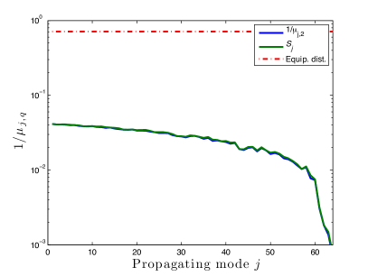
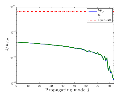
Discussion and numerical illustration. The decay of the mean mode amplitudes is a manifestation of the loss of coherence of the modes. This is a gradual process, with the last indexed modes losing coherence faster than the first ones, as illustrated by the numerical results displayed in Figure 2. We plot $\mathcal{S}_{j}=1/\mu_{j,1}$ in green and $1/\mu_{j,\mathfrak{M}_{j}}$ in blue. Note that $\mathcal{S}_{j}$ are the scaled scattering mean free paths, as follows from (75). The actual scattering mean free paths are given by $\mathcal{S}_{j}^{\epsilon}=\mathcal{S}_{j}/\epsilon^{2}$, and are much larger than the wavelength $\lambda$. The matrix ${\bf C}_{j}$ is computed as in (96), using the coefficients defined in appendix A, for an isotropic random medium that is stationary in $x_{1},x_{2}$ and $z$, with covariance

$${\mathbb{E}}[\nu(\vec{{\bf x}})\nu(\vec{{\bf x}}^{\prime})]={\rm exp}\left(-\frac{|\vec{{\bf x}}-\vec{{\bf x}}^{\prime}|^{2}}{2\ell^{2}}\right),\qquad\ell=\lambda.$$

The left plot is for a waveguide with dimensions $L_{1}=3.03\lambda$ and $L_{2}=5.84\lambda$, so that $N=64$. In the right plot $L_{1}=4.08\lambda$ and $L_{2}=5.77\lambda$, so that $N=84$.

Note that for any $j$ the eigenvalues $\mu_{j,s}$ are almost the same for $1\ll s\ll\mathfrak{M}_{j}$, indicating that the equality in (98) holds independent of the multiplicity $\mathfrak{M}_{j}$. Moreover, $\mathcal{S}_{j}$ decreases with $j$, and the rate of decrease acellerates for $j$ close to $N$. The scale shown with red in Figure 2 is the equipartition distance, up to the $\varepsilon^{-2}$ factor. This is the range where cumulative scattering by the medium distributes the energy of the waves uniformly over the modes, independent of their initial state. We give more details in the next section, but it is important to note that the equipartition distance is larger, by a factor of ten, than all the scattering mean free paths. This is very similar to the result obtained for sound waves in random waveguides with straight boundaries [3, Figure 4.2].

To interpret the results, let us note that the modes ${\boldsymbol{\varphi}}_{j}^{(s)}{\rm exp}(i\beta_{j}z)$, for $1\leq s\leq\mathfrak{M}_{j}$, are superpositions (component-wise) of the plane waves ${\rm exp}(i\vec{\bf K}_{j}\cdot\vec{{\bf x}})$, with wave vectors

$$\vec{\bf K}_{j}=\left(\pm{\pi j_{1}}/{L_{1}},\pm{\pi j_{2}}/{L_{2}},\beta_{j}\right),\qquad j=(j_{1},j_{2}).$$

The plus and minus signs are due to the reflections of the waves at the walls of the waveguide. Recall that $\beta_{j}=\sqrt{k^{2}-\lambda_{j}}$, with eigenvalues $\lambda_{j}$ defined by (23) and enumerated in increasing order. When $j$ is small, the wave vector $\vec{\bf K}_{j}$ is almost aligned with the range axis, and the waves propagate with large (group) range velocity

$${1}/{\beta^{\prime}_{j}(\omega)}=c_{o}\sqrt{1-{\lambda_{j}}/{k^{2}}}\approx c_{o}.$$

They arrive quickly to range $Z$ because they travel along shorter paths, with a small number of reflections at the walls, and are least affected by the random medium. For the high index modes $\lambda_{j}\approx k^{2}$, and the wave vectors $\vec{\bf K}_{j}$ are almost orthogonal to the range axis. The waves propagate very slowly along range because they strike the waveguide walls many times. The interaction with the random medium accumulates over the long travel paths of these modes, and the waves lose coherence over shorter range scales, as modeled by the small scattering mean free paths.

For any given $j$ the modes ${\boldsymbol{\varphi}}_{j}^{(s)}{\rm exp}(i\beta_{j}z)$ are the superposition of the same plane waves for $s=1$ and $2$, so their interaction with the medium is the same. This is why the eigenvalues $\mu_{j,1}$ and $\mu_{j,2}$ are almost equal.

7.5 The equipartition regime

The transport of energy in the waveguides is modeled by the evolution equations (92). Our goal in this section is to describe their solution in the limit $Z\to\infty$.

We begin by writing equations (92) as

$$\partial_{Z}{\bf P}(Z)=\Upsilon\big{(}\textbf{P}\big{)}(Z)=\Upsilon^{+}\big{(}\textbf{P}\big{)}(Z)-\Upsilon^{-}\big{(}\textbf{P}\big{)}(Z),\quad Z>0,$$ (101)

with initial condition ${\bf P}(0)={\bf P}_{o}$. Here $\Upsilon,\Upsilon^{\pm}:\mathfrak{X}\rightarrow\mathfrak{X}$ are linear operators acting on the vector space $\mathfrak{X}$ defined in section 7.3, with values in $\mathfrak{X}$. We have $\Upsilon=\Upsilon^{+}-\Upsilon^{-}$ and

$$\Upsilon^{+}\big{(}\textbf{P}\big{)}_{j}(Z)=\sum^{N}_{l=1}\Upsilon^{+}_{jl}\big{(}\textbf{P}_{l}\big{)}(Z)\,,\hskip 11.38092pt\Upsilon^{-}\big{(}\textbf{P}\big{)}_{j}(Z)=\sum^{N}_{l=1}\Upsilon^{-}_{jl}\big{(}{\bf P}_{j}\big{)}(Z),$$ (102)

with operators $\Upsilon^{\pm}_{jl}:\mathfrak{X}_{l}\rightarrow\mathfrak{X}_{j}$ acting on the spaces $\mathfrak{X}_{l}$ of Hermitian matrices defined in section 7.3, and given by

$$\Upsilon^{+}_{jl}\big{(}U\big{)} =\int_{-\infty}^{\infty}dz{\mathbb{E}}\left\{M_{AA,jl}(z)\,U\,M_{AA,jl}^{\star}(0)\right\}e^{i(\beta_{l}-\beta_{j})z}\,,$$

$$\Upsilon^{-}_{jl}\big{(}U\big{)} =-\Big{(}{\bf Q}_{l}\,U+U\,{\bf Q}_{l}^{\star}\Big{)}\delta_{jl}\,.$$ (103)

We may think of $\Upsilon^{+}_{jl}$ and $\Upsilon^{-}_{jl}$ as modeling the inflow/outflow of energy of the $j\leftrightarrows l$ modes, because

$$\Upsilon^{+}_{jl}(U)\geq 0\,\quad\text{and}\quad\text{trace}\big{(}\Upsilon^{-}_{jl}(U)\big{)}\geq 0\,,$$ (104)

for $1\leq l,j\leq N,$ and all $U\in\mathfrak{C}_{l}$, the cone of positive semidefinite matrices in $\mathfrak{X}_{l}$. The limit of ${\bf P}(Z)$ as $Z\to\infty$ depends on the spectrum of the operator $\Upsilon$, and in particular its kernel, described in the next theorem.

Theorem 6.

The operator $\Upsilon$ has the following spectral properties:
(i) The eigenvalues of $\Upsilon$ lie in $(-\infty,0]$.
(ii) The $\text{Kernel}\big{(}\Upsilon\big{)}$ is not trivial, it has an eigenbase, and it intersects the cone $\mathfrak{C}=\mathfrak{C}_{1}\times\mathfrak{C}_{2}\times\ldots\mathfrak{C}_{N}\subset\mathfrak{X}$.
(iii) The $\text{Kernel}\big{(}\Upsilon\big{)}$ is one dimensional under the additional assumption that

$$\Upsilon^{+}_{jl}\big{(}U\big{)}>0\,,\quad\forall\,0\neq U\in\mathfrak{C}_{l}~{}~{}{\rm and}~{}~{}1\leq j,l\leq N.$$ (105)

For any initial condition ${\bf P}_{o}\in\mathfrak{C}$ we have ${\bf P}(Z)\in\mathfrak{C}$ for all $Z$, as shown in appendix E. This is why we are interested in the cone $\mathfrak{C}$ of the space $\mathfrak{X}$. The assumption (105) says that there is positive flux of energy for all the waveguide modes. It is the generalization of the condition stated in [7, Section 20.3.3] which gives the equipartition regime for sound waves. The statement there is that the power spectral density of the fluctuations of the wave speed does not vanish when evaluated at the differences of the wavenumbers of the modes. Our condition (105) is similar, but with $\mathfrak{M}_{j}\times\mathfrak{M}_{j}$ matrices. The following corollary follows immediately from parts (i) and (iii) of Theorem 6.

Corollary 7.

Suppose that condition (105) holds, and let $\textbf{U}_{o}$ be the unique vector that spans $\text{Kernel}\big{(}\Upsilon\big{)}\cap\mathfrak{C}$, normalized by $\|\textbf{U}_{o}\|=\|\textbf{P}_{o}\|$. We have

$$\big{|}\textbf{P}(Z)-\textbf{U}_{o}\big{|}\leq C\,(1+Z)^{\mathfrak{m}_{{}_{\Upsilon}}}\,e^{\lambda_{{}_{\Upsilon}}\,Z},$$

where $\lambda_{{}_{\Upsilon}}$ is the smallest (in magnitude) nonzero eigenvalue of $\Upsilon$, and $\mathfrak{m}_{{}_{\Upsilon}}$ is its multiplicity.

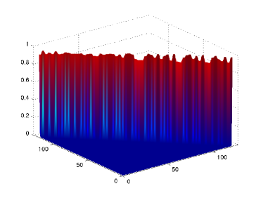
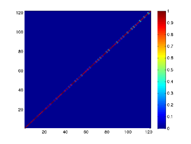
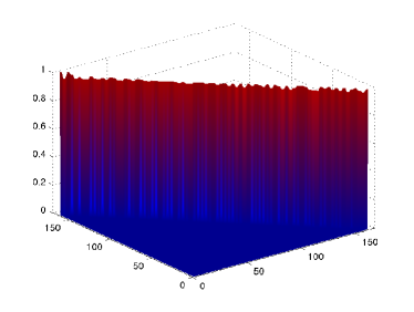
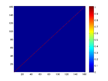
We display in Figure 3 the element ${\bf U}_{o}\in\text{Kernel}\big{(}\Upsilon\big{)}$ for the same two random waveguides considered in Figure 2. We normalize ${\bf U}_{o}$ so that its maximum entry is equal to one. Because ${\bf U}_{o}$ is a concatenation of $N$ matrices of size $\mathfrak{M}_{j}\times\mathfrak{M}_{j}$, we embed it in a square matrix for display purposes. The entries of interest in the square matrices displayed in Figure 3 are the $\mathfrak{M}_{j}\times\mathfrak{M}_{j}$ blocks along the diagonal. We note from the figure that the result is almost the matrix identity. Therefore, Corollary 7 says that in the limit $Z\to\infty$, the energy is distributed uniformly over the modes, independent of the initial mode power distribution ${\bf P}_{o}$. This is the equipartition regime, and it is reached when the waves travel beyond the equipartition distance

$$L_{\rm eq}=1/|\lambda_{{}_{\Upsilon}}|.$$ (106)

Fig. 3: The element (matrix) ${\bf U}_{o}\in\text{Kernel}\big{(}\Upsilon\big{)}$ for the same two waveguides considered in Figure 2. The top plots are for the waveguide with $N=64$ modes and the bottom plots for the waveguide with $N=84$ modes. We display ${\bf U}_{o}$ from the lateral side (left) to show the magnitude of its entries (left), and from above (right) to show that it is almost diagonal.

Proof of Theorem 6:

Item (i). Let $0\neq\lambda\in\mathbb{C}$ be an eigenvalue of $\Upsilon$ and $\textbf{U}\in\mathfrak{X}$ an associated eigenvector. Therefore, $\Upsilon\big{(}\textbf{U}\big{)}=\lambda\,\textbf{U}$, or componentwise,

$$\lambda\,U_{j}=\Upsilon\big{(}\textbf{U}\big{)}_{j}=\Upsilon\big{(}\textbf{U}\big{)}^{\star}_{j}=\big{(}\lambda\,U_{j}\big{)}^{\star}=\overline{\lambda}\,U_{j},\quad 1\leq j\leq N,$$

where we used definitions (102-7.5) to obtain the second equality. Consequently, the eigenvalues of $\Upsilon$ are real valued. To see that they cannot be positive, we use that $\textbf{P}(Z)\in\mathfrak{C}$ for all $Z$ as shown in appendix E, and the conservation of energy

$$\sum^{N}_{j=1}\text{trace}\big{(}\textbf{P}_{j}(Z)\big{)}=\sum^{N}_{j=1}\text{trace}\big{(}\textbf{P}_{j,o}\big{)}\,,\quad Z\geq 0.$$

Since $\textbf{P}_{j}(Z)\in\mathfrak{C}_{j}$, we have $0\leq P^{ss}_{j}(Z)\leq\text{trace}\big{(}\textbf{P}_{j}(Z)\big{)},$ for all $Z\geq 0$, $1\leq j\leq N$ and $1\leq s\leq\mathfrak{M}_{j}$. Moreover

$$\big{|}P^{12}_{j}(Z)\big{|}\leq\sqrt{P^{11}_{j}(Z)P^{22}_{j}(Z)}\leq\tfrac{1}{2}\text{trace}\big{(}\textbf{P}_{j}(Z)\big{)},\quad Z\geq 0,$$

when $\mathfrak{M}_{j}=2$, where we used the Cauchy-Schwarz inequality. Therefore

$$\sup_{Z\geq 0}\big{|}\textbf{P}(Z)\big{|}\leq\sum^{N}_{j=1}\text{trace}(\textbf{P}_{o}),\qquad\forall\,{\bf P}_{o}\in\mathfrak{C}.$$

Now consider an arbitrary initial state in $\mathfrak{X}$, not necessarily in $\mathfrak{C}$. We denote such a state by $\widetilde{{\bf P}}_{o}$ to distinguish it from a physical initial mode power state that is necessarily in $\mathfrak{C}$, and the corresponding solution of (101) by $\widetilde{P}(Z)$. Since any $\widetilde{\bf P}_{o}$ can be writen as a linear combination of elements in $\mathfrak{C}$, and (101) is linear, $\widetilde{P}(Z)$ is a linear combination of solutions with initial states in $\mathfrak{C}$, which are bounded as shown above. We conclude that all trajectories are bounded, independent of the initial state.

Now, let U be an eigenvector of $\Upsilon$ for an eigenvalue $\lambda$, and set $\widetilde{\bf P}_{0}=\textbf{U}$. The solution of (101) is $\widetilde{\bf P}(Z)=\textbf{U}\,e^{\lambda Z}$ and it is uniformly bounded if and only if $\lambda\leq 0$.

Item (ii). To characterize $\text{Kernel}(\Upsilon)$ we rewrite the conservation of energy as

$$\big{(}\Upsilon(\textbf{U}),\textbf{1}\big{)}_{\mathfrak{X}}=\big{(}\textbf{U},\Upsilon^{\star}(\textbf{1})\big{)}_{\mathfrak{X}}=0\,,\quad\forall\,\textbf{U}\in\mathfrak{X},$$ (107)

where 1 is the vector of concatenated $\mathfrak{M}_{j}\times\mathfrak{M}_{j}$ identity matrices, for $j=1,\ldots,N$, and $\Upsilon^{\star}$ is the adjoint of $\Upsilon$. We conclude that $\textbf{1}\in\text{Kernel}\big{(}\Upsilon^{*}\big{)}$, and therefore that the kernel of $\Upsilon$ is not trivial.

We also infer from the boundedness of the solutions of (101) that $\text{Kernel}\big{(}\Upsilon\big{)}$ has an eigenbase. Otherwise the solutions could grow polynomially in $Z$.

Now let us write the solutions of (101) as

$$\textbf{P}(Z)=\textbf{U}_{o}+\sum^{\mathfrak{n}}_{j=1}\sum^{\mathfrak{m}_{j}}_{q=0}c_{jq}\,\textbf{U}_{jq}\;(Z+1)^{q}e^{\lambda_{j}Z},$$ (108)

where $\textbf{U}_{o}\in\text{Kernel}\big{(}\Upsilon\big{)}$, and $n$ is the number of distinct eigenvalues $\lambda_{j}<0$ of $\Upsilon$, with multiplicity $m_{j}$. The finite sequences $\{\textbf{U}_{jq}\}^{\mathfrak{m}_{j}}_{q=1}$ are linear independent sets of generalized eigenvectors corresponding to the eigenvalue $\lambda_{j}$. Equation (108) implies

$$\big{|}\textbf{P}(Z)-\textbf{U}_{o}\big{|}\leq C\,(1+Z)^{\mathfrak{m}_{{}_{\Upsilon}}}\,e^{\lambda_{{}_{\Upsilon}}\,Z},$$ (109)

where we denote by $\lambda_{{}_{\Upsilon}}$ the eigenvalue with smallest magnitude and $m_{{}_{\Upsilon}}$ its multiplicity. Now, take $0\neq\textbf{P}_{o}\in\mathfrak{C}$, and therefore, $\textbf{P}(Z)\in\mathfrak{C}$ for all $Z\geq 0$. Letting $Z\rightarrow\infty$ in (109) we conclude that $\textbf{U}_{o}\in\mathfrak{C}$ i.e., $\textbf{U}_{o}\in\text{Kernel}\big{(}\Upsilon\big{)}\cap\mathfrak{C}$. Moreover, $\textbf{U}_{o}\neq 0$ by the conservation of energy.

Item (iii). We prove that condition (105) guarantees a one dimensional kernel of the adjoint operator $\Upsilon^{\star}$, and therefore of $\Upsilon$. We consider first a large family of linear mappings defined in terms of $\Upsilon^{*}$ and restricted to the subspace $\mathfrak{D}\subset\mathfrak{X}$ of vectors of diagonal matrices. We show that this family has the one dimensional kernel ${\rm span}\{{\bf 1}\}$ in $\mathfrak{D}$. Then we show that ${\rm Kernel}(\Upsilon^{\star})={\rm span}\{{\bf 1}\}$ in $\mathfrak{X}$.

To define the family of mappings, we recall that the elements ${\bf U}=(U_{1},\ldots,U_{N})$ of $\mathfrak{X}$ are vectors of Hermitian matrices which are diagonalized by similarity transformations with orthogonal matrices of their eigenvectors. For any vector $\textbf{V}=(V_{1},\ldots,V_{N})$ of orthogonal matrices we define the transformation $\varphi_{\textbf{V}}:\mathfrak{X}\rightarrow\mathfrak{X}$ by

$$\varphi_{\textbf{V}}\big{(}\textbf{U}\big{)}=\textbf{V}^{\star}\,\textbf{U}\,\textbf{V}:=\big{(}V^{\star}_{1}U_{1}V_{1},\cdots,V^{\star}_{N}U_{N}V_{N}\big{)},$$

with dimensions of $U_{j}$ and $V_{j}$ assumed to match for each $1\leq j\leq N$. We also define the family of operators $\Upsilon^{\star}_{\textbf{V}}:\mathfrak{X}\rightarrow\mathfrak{X}$ by $\Upsilon^{\star}_{\textbf{V}}=\varphi_{\textbf{V}}^{-1}\circ\Upsilon^{\star}\circ\varphi_{\textbf{V}}$, or more explicitly,

$$\Upsilon^{\star}_{\textbf{V}}\big{(}\textbf{U}\big{)}=\textbf{V}\,\Upsilon^{\star}\big{(}\textbf{V}^{\star}\,\textbf{U}\,\textbf{V}\big{)}\,\textbf{V}^{\star}\,,\quad\textbf{U}\in\mathfrak{X}.$$ (110)

Its restriction to the subspace $\mathfrak{D}\subset\mathfrak{X}$ of vectors of diagonal matrices is denoted by

$$\Upsilon^{\star}_{\textbf{V}\big{|}\mathfrak{D}}\big{(}\textbf{D}\big{)}=\Upsilon^{\star}_{\textbf{V}}\big{(}\textbf{D}\big{)}\,\quad\text{for any}\;\;\textbf{D}\in\mathfrak{D},$$

and we wish to prove that

$${\rm Kernel}\big{(}\Upsilon^{\star}_{\textbf{V}\big{|}\mathfrak{D}}\big{)}={\rm span}\{{\bf 1}\},\qquad\forall\,{\bf V}.$$ (111)

Note that $\Upsilon^{\star}_{\textbf{V}\big{|}\mathfrak{D}}(\textbf{1})=0$ by the definition (110) and $\Upsilon^{\star}({\bf 1})=0$.

The statement of the theorem is implied by (111). Indeed, take an arbitrary $\textbf{U}\in\text{Kernel}\big{(}\Upsilon^{\star}\big{)}$. Since $\mathbf{U}$ is a vector of Hermitian matrices, there exists a vector V of orthogonal matrices and a vector D of diagonal matrices such that $\textbf{U}=\textbf{V}^{*}\,\textbf{D}\textbf{V}$. Then $\textbf{D}\in\text{Kernel}\big{(}\Upsilon^{\star}_{\textbf{V}\big{|}\mathfrak{D}}\big{)}$ and (111) implies that $\textbf{D}=\alpha\,\mathbf{1}$ for some $\alpha\in\mathbb{R}$. Consequently,

$$\textbf{U}={\bf V}^{\star}\alpha{\bf 1}{\bf V}=\alpha\,\mathbf{1},$$

which means that ${\rm Kernel}(\Upsilon^{\star})={\rm span}\{{\bf 1}\}$.

The proof of (111) is based on the Perron–Frobenius theorem for irreducible matrices. We start by computing the matrix representation of the operator $\Upsilon^{\star}_{\textbf{V}}$ using the properties of the adjoint operators $\Upsilon^{\pm\,\star}_{jl}:\mathfrak{X}_{j}\rightarrow\mathfrak{X}_{l}$ that define $\Upsilon^{\star}$. Then, we extract a suitable irreducible matrix $\Lambda_{\textbf{V}}$ from it to apply the Perron–Frobenius theorem.

The matrix representation of $\Upsilon^{\star}_{\textbf{V}}$ consists of $N^{2}$ blocks, where the $lj$–block is the matrix representation of the operator $\Upsilon^{+\star}_{\textbf{V}lj}-\Upsilon^{-\star}_{\textbf{V}lj}$, with $\Upsilon^{\pm\star}_{\textbf{V}lj}:\mathfrak{X}_{j}\rightarrow\mathfrak{X}_{l}$ defined naturally, in light of (110), as

$$\Upsilon^{\pm\star}_{\textbf{V}lj}(U)=V_{l}\,\Upsilon^{\pm\,\star}_{jl}\big{(}V^{\star}_{j}\,U\,V_{j}\big{)}\,V^{\star}_{l}\,,\quad U\in\mathfrak{X}_{j}.$$

Recall that the dimension of $\mathfrak{X}_{j}$ is $\mathfrak{M}^{2}_{j}$, so the $lj$–block has dimension $\mathfrak{M}^{2}_{l}\times\mathfrak{M}^{2}_{j}$. To be more precise, consider the case $\mathfrak{M}_{j}=\mathfrak{M}_{l}=2$, and write explicitly

$$\Upsilon^{\pm\star}_{\textbf{V}lj}=\Big{(}\upsilon^{\pm\,ss^{\prime}}_{lj}\Big{)}\,,\quad 1\leq s\leq\mathfrak{M}^{2}_{l}\,,\quad 1\leq s^{\prime}\leq\mathfrak{M}^{2}_{j},$$

In terms of the canonical basis for $\mathfrak{X}_{j}$

$$\left\{\Big{(}\begin{array}[]{cc}1&0\\ 0&0\end{array}\Big{)},\Big{(}\begin{array}[]{cc}0&0\\ 0&1\end{array}\Big{)},\tfrac{1}{\sqrt{2}}\Big{(}\begin{array}[]{cc}0&1\\ 1&0\end{array}\Big{)},\tfrac{1}{\sqrt{2}}\Big{(}\begin{array}[]{cc}0&i\\ -i&0\end{array}\Big{)}\right\}=:\big{\{}E_{1},E_{2},E_{3},E_{4}\big{\}},$$

we have

$$\upsilon^{+\,ss^{\prime}}_{lj} =\big{(}E_{s},\Upsilon^{+\star}_{\textbf{V}{lj}}(E_{s^{\prime}})\big{)}_{\mathfrak{X}_{l}}$$

$$=\big{(}E_{s},V_{l}\,\Upsilon^{+\,\star}_{jl}\big{(}V^{\star}_{j}\,E_{s^{\prime}}\,V_{j}\big{)}\,V^{\star}_{l}\big{)}_{\mathfrak{X}_{l}}$$

$$=\big{(}V^{\star}_{l}\,E_{s}\,V_{l},\Upsilon^{+\,\star}_{jl}\big{(}V^{\star}_{j}\,E_{s^{\prime}}\,V_{j}\big{)}\big{)}_{\mathfrak{X}_{l}}.$$ (112)

Note that $E_{1}$ and $E_{2}$ are positive semidefinite matrices, and so are $V^{\star}_{l}\,E_{1}\,V_{l}$ and $V^{\star}_{j}\,E_{2}\,V_{j}$. It follows from the explicit expression of $\Upsilon^{+\,\star}_{jl}$ computed from (7.5) as

$$\Upsilon^{{+\,\star}}_{jl}(U)=\int_{-\infty}^{\infty}dz\,{\mathbb{E}}\left\{M_{{AA,jl}}^{\star}(z)UM_{AA,jl}(0)\right\}e^{-i(\beta_{l}-\beta_{j})z},$$ (113)

and equation (7.5), that

$$\upsilon^{+\,ss^{\prime}}_{lj}\geq 0\,,\quad 1\leq s,s^{\prime}\leq 2.$$ (114)

The remaining entries of $\Upsilon^{+\star}_{\textbf{V}lj}$ do not have a definite sign, in general. The entries of $\Upsilon^{-\star}_{\textbf{V}lj}$ are computed similarly, and take the form

$$\upsilon^{-\,ss^{\prime}}_{lj} =\big{(}E_{s},\Upsilon^{-\star}_{\textbf{V}{lj}}(E_{s^{\prime}})\big{)}_{\mathfrak{X}_{l}}$$

$$=\big{(}E_{s},V_{l}\,\Upsilon^{-\,\star}_{jl}\big{(}V^{\star}_{j}\,E_{s^{\prime}}\,V_{j}\big{)}\,V^{\star}_{l}\big{)}_{\mathfrak{X}_{l}}$$

$$=\big{(}E_{s},\big{(}V_{l}\,\textbf{C}_{l}\,V^{\star}_{l}\big{)}\,E_{s}\big{)}_{\mathfrak{X}_{l}}\,\delta_{ss^{\prime}}\,\delta_{jl}\geq 0\,,\quad 1\leq s,s^{\prime}\leq 2.$$ (115)

We used that $E_{s}E_{s^{\prime}}=E_{s}\delta_{ss^{\prime}}$ for $s,s^{\prime}\in\{1,2\}$ for the third equality, and properties of positive definite matrices in the last inequality. In summary, the $lj$–block is of the form

$$\Big{(}\upsilon^{+\,ss^{\prime}}_{lj}\Big{)}-\Big{(}\upsilon^{-\,ss^{\prime}}_{lj}\Big{)}=\Bigg{(}\begin{array}[]{cc}\boldsymbol{\upsilon}^{+}_{lj}&\cdot\\ \cdot&\cdot\end{array}\Bigg{)}-\Bigg{(}\begin{array}[]{cc}\boldsymbol{\upsilon}^{-}_{ll}&\cdot\\ \cdot&\cdot\end{array}\Bigg{)}\,\delta_{lj},$$ (116)

with $2\times 2$ matrices $\boldsymbol{\upsilon}^{\pm}_{lj}$ with nonnegative entries, and nonnegative diagonal matrices $\boldsymbol{\upsilon}^{-}_{ll}$. Cases where $\mathfrak{M}_{j}$ or $\mathfrak{M}_{l}$ or both are equal to one are handled similarly.

Now, define the $\mathfrak{M}\times\mathfrak{M}$ square matrix

$$\Lambda_{\textbf{V}}=\text{Block}\big{(}\boldsymbol{\upsilon}^{+}_{lj}\big{)}-\text{Block}\big{(}\boldsymbol{\upsilon}^{-}_{lj}\big{)},$$ (117)

where $\mathfrak{M}=\displaystyle\sum_{j=1}^{N}\mathfrak{M}_{j}$, and observe that the dimension of its kernel satisfies

$$1\leq\text{Dim}\big{\{}\text{Kernel}\big{(}\Upsilon^{\star}_{\textbf{V}\big{|}\mathfrak{D}}\big{)}\big{\}}\leq\text{Dim}\big{\{}\text{Kernel}\big{(}\Lambda_{\textbf{V}}\big{)}\big{\}}.$$ (118)

This is because for any $\textbf{D}\in\text{Kernel}\big{(}\Upsilon^{\star}_{\textbf{V}\big{|}\mathfrak{D}}\big{)}$, by construction of $\Lambda_{\textbf{V}}$, the $\mathfrak{M}$ vector formed by the diagonal entries of D lies in $\text{Kernel}\big{(}\Lambda_{\textbf{V}}\big{)}$. In particular, $\big{(}1,1,\cdots,1\big{)}\in\text{Kernel}\big{(}\Lambda_{\textbf{V}}\big{)}$ so the entries in each row of $\Lambda_{\textbf{V}}$ sum to zero. Then, Gershgorin’s circle theorem and the special structure of $\Lambda_{\textbf{V}}$ give that any eigenvalue $\lambda_{\textbf{V}}$ of $\Lambda_{\textbf{V}}$ satisfies

$$\lambda_{\textbf{V}}\leq v_{jj}^{+ss}-v_{jj}^{-}+v_{jj}^{+ss^{\prime}}+\sum_{l\neq j}\sum_{s^{\prime\prime}=1}^{\mathfrak{M}_{l}}v_{jl}^{+ss^{\prime\prime}}=0,$$

for all $1\leq s,s^{\prime}\leq\mathfrak{M}_{j}$ and $s\neq s^{\prime}$. This shows that the largest eigenvalue of $\lambda_{\textbf{V}}$ is zero.

Consider now the matrix

$$\Lambda_{\textbf{V}}+\alpha\textbf{I},$$

with $\alpha$ a sufficiently large positive real number such that the diagonal is positive. The spectrum of this matrix is a translation by $\alpha$ of the spectrum of $\Lambda_{\textbf{V}}$, therefore, by the previous discussion $\alpha$ must be its largest positive real eigenvalue. Assuming that $\text{Block}\big{(}\boldsymbol{\upsilon}^{+}_{lj}\big{)}$ is irreducible, $\Lambda_{\textbf{V}}+\alpha\textbf{I}$ is a Perron–Frobenius matrix implying that its largest positive real eigenvalue, in this case $\alpha$, is simple, and therefore, zero is a simple eigenvalue of $\Lambda_{\textbf{V}}$. Thus, the kernel of $\Lambda_{\textbf{V}}$ is one dimensional and so is the kernel of $\Upsilon^{\star}_{\textbf{V}\big{|}\mathfrak{D}}$, by (118). This is precisely (111).

It remains to show that the condition (105) ensures that $\text{Block}\big{(}\boldsymbol{\upsilon}^{+}_{lj}\big{)}$ is irreducible, regardless of the transformation $\varphi_{\textbf{V}}$. We already know that this is a matrix with nonnegative entries, but we need to show that each entry is positive. From (7.5) we observe that this means that

$$\upsilon^{+,ss^{\prime}}_{lj}=\text{trace}\Big{(}E_{s}\,V_{l}\,\Upsilon^{+\,\star}_{jl}\big{(}V^{\star}_{j}\,E_{s^{\prime}}\,V_{j}\big{)}\,V^{\star}_{l}\Big{)}>0\,,\quad 1\leq s\leq\mathfrak{M}_{l},\;\;1\leq s^{\prime}\leq\mathfrak{M}_{j},$$

which is equivalent to saying that the diagonal entries of the matrix

$$V_{l}\,\Upsilon^{+\,\star}_{jl}\big{(}V^{\star}_{j}\,E_{s^{\prime}}\,V_{j}\big{)}\,V^{\star}_{l}\,,\quad 1\leq s^{\prime}\leq\mathfrak{M}_{j},$$

are positive. To see that this is true, observe that $0\neq V^{\star}_{j}\,E_{s^{\prime}}\,V_{j}\in\mathfrak{C}_{j}$ for $1\leq s^{\prime}\leq\mathfrak{M}_{j}$, and that condition (105) and definition (113) imply

$$\Upsilon^{+\,\star}_{jl}\big{(}V^{\star}_{j}\,E_{s^{\prime}}\,V_{j}\big{)}>0\,,\quad 1\leq s^{\prime}\leq\mathfrak{M}_{j}.$$

The result follows immediately from this. $\Box$

8 Summary

We presented a rigorous analysis of electromagnetic wave propagation in waveguides with rectangular cross-section. The dielectric materials that fill the waveguides are lossless isotropic, and contain numerous weak inhomogeneities (imperfections). Consequently, their electric permittivity $\varepsilon(\vec{{\bf x}})$ has small fluctuations in $\vec{{\bf x}}$ that are uncertain in applications, which is why we model them with a random process. The main result of the paper is a detailed characterization of long range cumulative scattering effects in random waveguides.

Our method of analysis decomposes the electromagnetic wave field in transverse electric and magnetic modes, which are propagating and evanescent waves. The modes are coupled by scattering in the random medium, so their amplitudes are random processes. They satisfy a stochastic system of equations driven by the random fluctuations of the permittivity $\varepsilon(\vec{{\bf x}})$, and can be analyzed at long range using the diffusion approximation theorem. The result is a detailed characterization of the loss of coherence of the modes, the depolarization of the waves due to scattering, and the transport of energy by the modes. Loss of coherence means that the expectation of the mode amplitudes (the coherent part) is overwhelmed by their random fluctuations (the incoherent part) once the waves travel beyond distances called scattering mean free paths. These are range scales that depend on the modes, the wavelength and the covariance of the fluctuations of $\varepsilon(\vec{{\bf x}})$. Our analysis of long range transport of energy shows how scattering in the random medium redistributes the energy among the waveguide modes. In particular, it identifies a range scale, called the equipartition distance, beyond which the energy is uniformly distributed among the waveguide modes, independent of the initial conditions.

Our results have applications in long range communications and imaging in waveguides. See for example the imaging and time reversal studies [4, 3, 8] that are based on the theory of sound wave propagation in random waveguides developed in [14, 6, 9, 1, 2]. Here we extended the theory to electromagnetic wave propagation in random waveguides.

Appendix A The coupling coefficients

Let us denote by

$$\mathbb{O}_{{\bf D}{\bf D}}^{\epsilon}=\left[\partial_{z}\nu(\vec{{\bf x}})-\frac{\epsilon}{2}\partial_{z}\nu^{2}(\vec{{\bf x}})\right]I\,,$$ (119)

and

$$\mathbb{O}_{{\bf D}{\bf U}}^{\epsilon}=ik\nu(\vec{{\bf x}}){\bf I}-\frac{i}{k}\nabla\nu(\vec{{\bf x}})\nabla\cdot+\frac{i\epsilon}{2k}\nabla\nu^{2}(\vec{{\bf x}})\nabla\cdot\,,$$ (120)

the perturbation operators in (56) acting on ${\bf D}$ and ${\bf U}$, where ${\bf I}$ is the identity. Similarly, we let $\mathbb{O}_{{\bf U}{\bf D}}^{\epsilon}$ be the perturbation operator in (57) acting on ${\bf U}$. The coupling coefficients in equations (64-65) are linear combinations of

$$\alpha_{jj^{\prime}}^{(ss^{\prime})\epsilon}(z) =\left(\sqrt{\frac{\beta_{j}}{k}}\delta_{s1}+\sqrt{\frac{k}{\beta_{j}}}\delta_{s2}\right)\left<{\boldsymbol{\varphi}}_{j}^{(s)},\mathbb{O}_{{\bf D}{\bf D}}^{\epsilon}{\boldsymbol{\varphi}}_{j^{\prime}}^{(s^{\prime})}\right>\left(\sqrt{\frac{k}{\beta_{j^{\prime}}}}\delta_{s^{\prime}1}+\sqrt{\frac{\beta_{j^{\prime}}}{k}}\delta_{s^{\prime}2}\right)\,,$$

$$\gamma_{jj^{\prime}}^{(ss^{\prime})\epsilon}(z) =\left(\sqrt{\frac{\beta_{j}}{k}}\delta_{s1}+\sqrt{\frac{k}{\beta_{j}}}\delta_{s2}\right)\left<{\boldsymbol{\varphi}}_{j}^{(s)},\mathbb{O}_{{\bf D}{\bf U}}^{\epsilon}{\boldsymbol{\varphi}}_{j^{\prime}}^{(s^{\prime})}\right>\left(\sqrt{\frac{\beta_{j^{\prime}}}{k}}\delta_{s^{\prime}1}+\sqrt{\frac{k}{\beta_{j^{\prime}}}}\delta_{s^{\prime}2}\right)\,,$$

$$\eta_{jj^{\prime}}^{(ss^{\prime})\epsilon}(z) =\left(\sqrt{\frac{k}{\beta_{j}}}\delta_{s1}+\sqrt{\frac{\beta_{j}}{k}}\delta_{s2}\right)\left<{\boldsymbol{\varphi}}_{j}^{(s)},\mathbb{O}_{{\bf U}{\bf D}}^{\epsilon}{\boldsymbol{\varphi}}_{j^{\prime}}^{(s^{\prime})}\right>\left(\sqrt{\frac{k}{\beta_{j^{\prime}}}}\delta_{s^{\prime}1}+\sqrt{\frac{\beta_{j^{\prime}}}{k}}\delta_{s^{\prime}2}\right)\,,$$

where $\left<\cdot,\cdot\right>$ denotes inner product in $L^{2}(\Omega)$. These expressions become after integration by parts

$$\alpha_{jj^{\prime}}^{(ss^{\prime})\epsilon}(z)= \left(\sqrt{\frac{\beta_{j}}{k}}\delta_{s1}+\sqrt{\frac{k}{\beta_{j}}}\delta_{s2}\right)\left(\sqrt{\frac{k}{\beta_{j^{\prime}}}}\delta_{s^{\prime}1}+\sqrt{\frac{\beta_{j^{\prime}}}{k}}\delta_{s^{\prime}2}\right)\times$$

$$\left[\partial_{z}\Psi_{jj^{\prime}}^{(ss^{\prime})}(z)-\frac{\epsilon}{2}\partial_{z}\psi_{jj^{\prime}}^{(ss^{\prime})}(z)\right]\,,$$ (121)

and

$$\gamma_{jj^{\prime}}^{(ss^{\prime})\epsilon}(z)= \frac{i}{k}\left(\sqrt{\frac{\beta_{j}}{k}}\delta_{s1}+\sqrt{\frac{k}{\beta_{j}}}\delta_{s2}\right)\left(\sqrt{\frac{\beta_{j^{\prime}}}{k}}\delta_{s^{\prime}1}+\sqrt{\frac{k}{\beta_{j^{\prime}}}}\delta_{s^{\prime}2}\right)\times$$

$$\left\{(k^{2}-\lambda_{j^{\prime}}\delta_{s^{\prime}2})\Psi_{jj^{\prime}}^{(ss^{\prime})}(z)+\Theta_{jj^{\prime}}^{(ss^{\prime})}(z)+\frac{\epsilon}{2}\left[\lambda_{j^{\prime}}\delta_{s^{\prime}2}\psi_{jj^{\prime}}^{(ss^{\prime})}(z)-\theta_{jj^{\prime}}^{(ss^{\prime})}(z)\right]\right\}\,,$$ (122)

and

$$\eta_{jj^{\prime}}^{(ss^{\prime})\epsilon}(z)=\frac{i\lambda_{j}\delta_{s1}}{\sqrt{k\beta_{j}}}\left(\sqrt{\frac{k}{\beta_{j^{\prime}}}}\delta_{s^{\prime}1}+\sqrt{\frac{\beta_{j^{\prime}}}{k}}\delta_{s^{\prime}2}\right)\left[\Psi_{jj^{\prime}}^{(ss^{\prime})}(z)-\epsilon\psi_{jj^{\prime}}^{(ss^{\prime})}(z)\right]\,,$$ (123)

where we introduced the notation

$$\Psi_{jj^{\prime}}^{(ss^{\prime})}(z) =\int_{\Omega}d{\bf x}\,\nu(\vec{{\bf x}})\phi_{j}^{(s)}({\bf x})\cdot\phi_{j^{\prime}}^{(s^{\prime})}({\bf x})\,,$$

$$\psi_{jj^{\prime}}^{(ss^{\prime})}(z) =\int_{\Omega}d{\bf x}\,\nu^{2}(\vec{{\bf x}})\phi_{j}^{(s)}({\bf x})\cdot\phi_{j^{\prime}}^{(s^{\prime})}({\bf x})\,,$$ (124)

and

$$\Theta_{jj^{\prime}}^{(ss^{\prime})}(z) =\int_{\Omega}d{\bf x}\,\nu(\vec{{\bf x}})\,\nabla\cdot\phi_{j}^{(s)}({\bf x})\nabla\cdot\phi_{j^{\prime}}^{(s^{\prime})}({\bf x})\,,$$

$$\theta_{jj^{\prime}}^{(ss^{\prime})}(z) =\int_{\Omega}d{\bf x}\,\nu^{2}(\vec{{\bf x}})\,\nabla\cdot\phi_{j}^{(s)}({\bf x})\nabla\cdot\phi_{j^{\prime}}^{(s^{\prime})}({\bf x})\,.$$ (125)

Note that since $\nabla\cdot\phi_{j}^{(1)}=0$, we have

$$\Theta_{jj^{\prime}}^{(ss^{\prime})}(z)=\delta_{s2}\delta_{s^{\prime}2}\Theta_{jj^{\prime}}^{(22)}(z)\,,$$ (126)

and similar for $\theta_{jj^{\prime}}^{(ss^{\prime})}(z)$.

The coupling coefficients in (64) are given by

$$M_{AA,jj^{\prime}}^{(ss^{\prime})}(z)+\epsilon\,m_{AA,jj^{\prime}}^{(ss^{\prime})}(z) =\frac{1}{2}\left[\alpha_{jj^{\prime}}^{(ss^{\prime})\epsilon}(z)+\gamma_{jj^{\prime}}^{(ss^{\prime})\epsilon}(z)+\eta_{jj^{\prime}}^{(ss^{\prime})\epsilon}(z)\right]\,,$$ (127)

$$M_{AB,jj^{\prime}}^{(ss^{\prime})}(z)+\epsilon\,m_{AB,jj^{\prime}}^{(ss^{\prime})}(z) =\frac{1}{2}\left[\alpha_{jj^{\prime}}^{(ss^{\prime})\epsilon}(z)-\gamma_{jj^{\prime}}^{(ss^{\prime})\epsilon}(z)+\eta_{jj^{\prime}}^{(ss^{\prime})\epsilon}(z)\right]\,,$$ (128)

$$M_{AV,jj^{\prime}}^{(ss^{\prime})}(z)+\epsilon\,m_{AV,jj^{\prime}}^{(ss^{\prime})}(z) =\frac{1}{2}\left[\alpha_{jj^{\prime}}^{(ss^{\prime})\epsilon}(z)+\eta_{jj^{\prime}}^{(ss^{\prime})\epsilon}(z)\right]\,,$$ (129)

$$M_{Av,jj^{\prime}}^{(ss^{\prime})}(z)+\epsilon\,m_{Av,jj^{\prime}}^{(ss^{\prime})}(z) =-\frac{i}{2}(-1)^{s^{\prime}}\gamma_{jj^{\prime}}^{(ss^{\prime})\epsilon}(z)\,,$$ (130)

and those in (65) are

$$M_{BA,jj^{\prime}}^{(ss^{\prime})}(z)+\epsilon\,m_{BA,jj^{\prime}}^{(ss^{\prime})}(z) =\frac{1}{2}\left[\alpha_{jj^{\prime}}^{(ss^{\prime})\epsilon}(z)+\gamma_{jj^{\prime}}^{(ss^{\prime})\epsilon}(z)-\eta_{jj^{\prime}}^{(ss^{\prime})\epsilon}(z)\right]\,,$$ (131)

$$M_{BB,jj^{\prime}}^{(ss^{\prime})}(z)+\epsilon\,m_{BB,jj^{\prime}}^{(ss^{\prime})}(z) =\frac{1}{2}\left[\alpha_{jj^{\prime}}^{(ss^{\prime})\epsilon}(z)-\gamma_{jj^{\prime}}^{(ss^{\prime})\epsilon}(z)-\eta_{jj^{\prime}}^{(ss^{\prime})\epsilon}(z)\right]\,,$$ (132)

$$M_{BV,jj^{\prime}}^{(ss^{\prime})}(z)+\epsilon\,m_{BV,jj^{\prime}}^{(ss^{\prime})}(z) =\frac{1}{2}\left[\alpha_{jj^{\prime}}^{(ss^{\prime})\epsilon}(z)-\eta_{jj^{\prime}}^{(ss^{\prime})\epsilon}(z)\right]\,,$$ (133)

$$M_{Bv,jj^{\prime}}^{(ss^{\prime})}(z)+\epsilon\,m_{Bv,jj^{\prime}}^{(ss^{\prime})}(z) =-\frac{i}{2}(-1)^{s^{\prime}}\gamma_{jj^{\prime}}^{(ss^{\prime})\epsilon}(z)\,.$$ (134)

Because $\gamma_{jj^{\prime}}^{(ss^{\prime})\epsilon}(z)$ and $\eta_{jj^{\prime}}^{(ss^{\prime})\epsilon}(z)$ are imaginary, we obtain the relations

$$M_{BB,jj^{\prime}}^{(ss^{\prime})}(z) =\overline{M_{AA,jj^{\prime}}^{(ss^{\prime})}(z)}\,,\qquad m_{BB,jj^{\prime}}^{(ss^{\prime})}(z)=\overline{m_{AA,jj^{\prime}}^{(ss^{\prime})}(z)}\,,$$ (135)

$$M_{BA,jj^{\prime}}^{(ss^{\prime})}(z) =\overline{M_{AB,jj^{\prime}}^{(ss^{\prime})}(z)}\,,\qquad m_{BA,jj^{\prime}}^{(ss^{\prime})}(z)=\overline{m_{AB,jj^{\prime}}^{(ss^{\prime})}(z)}\,,$$ (136)

$$M_{BV,jj^{\prime}}^{(ss^{\prime})}(z) =\overline{M_{AV,jj^{\prime}}^{(ss^{\prime})}(z)}\,,\qquad m_{BV,jj^{\prime}}^{(ss^{\prime})}(z)=\overline{m_{AV,jj^{\prime}}^{(ss^{\prime})}(z)}\,,$$ (137)

$$M_{Bv,jj^{\prime}}^{(ss^{\prime})}(z) =\overline{M_{Av,jj^{\prime}}^{(ss^{\prime})}(z)}\,,\qquad m_{Bv,jj^{\prime}}^{(ss^{\prime})}(z)=\overline{m_{Av,jj^{\prime}}^{(ss^{\prime})}(z)}\,.$$ (138)

Similarly, the coupling coefficients in equations (66-67) satisfied by the evanescent modes are given by

$$M_{VA,jj^{\prime}}^{(ss^{\prime})}(z)+\epsilon\,m_{VA,jj^{\prime}}^{(ss^{\prime})}(z) =\alpha_{jj^{\prime}}^{(ss^{\prime})\epsilon}(z)+\gamma_{jj^{\prime}}^{(ss^{\prime})\epsilon}(z)\,,$$ (139)

$$M_{vA,jj^{\prime}}^{(ss^{\prime})}(z)+\epsilon\,m_{vA,jj^{\prime}}^{(ss^{\prime})}(z) =i(-1)^{s}\eta_{jj^{\prime}}^{(ss^{\prime})\epsilon}(z)\,,$$ (140)

$$M_{VV,jj^{\prime}}^{(ss^{\prime})}(z)+\epsilon\,m_{VV,jj^{\prime}}^{(ss^{\prime})}(z) =\alpha_{jj^{\prime}}^{(ss^{\prime})\epsilon}(z)\,,$$ (141)

$$M_{Vv,jj^{\prime}}^{(ss^{\prime})}(z)+\epsilon\,m_{Vv,jj^{\prime}}^{(ss^{\prime})}(z) =-i(-1)^{s^{\prime}}\gamma_{jj^{\prime}}^{(ss^{\prime})\epsilon}(z)\,,$$ (142)

$$M_{vV,jj^{\prime}}^{(ss^{\prime})}(z)+\epsilon\,m_{Vv,jj^{\prime}}^{(ss^{\prime})}(z) =i(-1)^{s}\eta_{jj^{\prime}}^{(ss^{\prime})\epsilon}(z)\,,$$ (143)

and by

$$M_{VB,jj^{\prime}}^{(ss^{\prime})}(z) =\overline{M_{VA,jj^{\prime}}^{(ss^{\prime})}(z)}\,,\qquad m_{VB,jj^{\prime}}^{(ss^{\prime})}(z)=\overline{m_{VA,jj^{\prime}}^{(ss^{\prime})}(z)}\,,$$ (144)

$$M_{vB,jj^{\prime}}^{(ss^{\prime})}(z) =\overline{M_{vA,jj^{\prime}}^{(ss^{\prime})}(z)}\,,\qquad m_{vB,jj^{\prime}}^{(ss^{\prime})}(z)=\overline{m_{vA,jj^{\prime}}^{(ss^{\prime})}(z)}\,.$$ (145)

In equations (66-67) we use only the leading part of these coefficients denoted by the capital letter $M$, as in $M_{VA,jj^{\prime}}^{(ss^{\prime})}(z)$.

Appendix B Analysis of the evanescent modes

Consider the $2\times 2$ system

$$\partial_{z}{\boldsymbol{\mathcal{V}}}_{j}^{(s)}(z)+\beta_{j}\left(\begin{array}[]{cc}0{}{}&1\\ 1{}{}&0\end{array}\right){\boldsymbol{\mathcal{V}}}_{j}^{(s)}(z)=\epsilon{\boldsymbol{\mathcal{F}}}_{j}^{(s)}(z,{\boldsymbol{\mathcal{V}}})\,,$$ (146)

for vectors

$${\boldsymbol{\mathcal{V}}}_{j}^{(s)}(z)=\left(\begin{array}[]{c}V_{j}^{(s)}(z)\\ v_{j}^{(s)}(z)\end{array}\right)\,,$$ (147)

which we string together in the infinite vector ${\boldsymbol{\mathcal{V}}}(z)$. The system (66-67) is of this form, with right hand-side

$${\boldsymbol{\mathcal{F}}}_{j}^{(s)}(z,{\boldsymbol{\mathcal{V}}})=\left(\begin{array}[]{c}F_{j}^{(s)}(z)\\ f_{j}^{(s)}(z)\end{array}\right)+\sum_{j^{\prime}>N}\sum_{s^{\prime}=1}^{\mathfrak{M}_{j^{\prime}}}\left(\begin{array}[]{cc}M_{VV,jj^{\prime}}^{(ss^{\prime})}(z){}{}&M_{Vv,jj^{\prime}}^{(ss^{\prime})}(z)\\ M_{vV,jj^{\prime}}^{(ss^{\prime})}(z)&0\end{array}\right){\boldsymbol{\mathcal{V}}}_{j^{\prime}}^{(s^{\prime})}(z)\,.$$ (148)

We neglect the $O(\epsilon^{2})$ remainder because it plays no role in our setup.

We diagonalize (146) by writing ${\boldsymbol{\mathcal{V}}}^{(s)}_{j}$ in the orthonormal basis $\{{\bf u}^{+},~{}{\bf u}^{-}\}$ of $\mathbb{R}^{2}$, where ${\bf u}^{\pm}=\frac{1}{\sqrt{2}}\left(\begin{array}[]{c}1\\ \pm 1\end{array}\right)\,$ are the eigenvectors of matrix $\left(\begin{array}[]{cc}0{}{}&1\\ 1{}{}&0\end{array}\right)$ for eigenvalues $\pm 1$. Explicitly, we write

$${\boldsymbol{\mathcal{V}}}_{j}^{(s)}(z)=\theta_{j}^{(s)+}(z){\bf u}^{+}+\theta_{j}^{(s)-}(z){\bf u}^{-}\,,$$ (149)

where $\theta_{j}^{(s)\pm}(z)$ are decaying and growing evanescent waves, satisfying

$$\left[\partial_{z}\pm\beta_{j}\right]\theta_{j}^{(s)\pm}(z)=\epsilon{\bf u}^{\pm}\cdot{\boldsymbol{\mathcal{F}}}_{j}^{(s)}(z,{\boldsymbol{\mathcal{V}}})\,,$$ (150)

the initial condition

$$\theta_{j}^{(s)+}(0+)={\bf u}^{+}\cdot{\boldsymbol{\mathcal{V}}}_{j}^{(s)}(0+)=\sqrt{2}E_{j,o}^{(s)}\,,$$ (151)

and the end condition

$$\theta_{j}^{(s)-}(z_{\rm max})=0.$$ (152)

We obtain after integrating equations (150) and using (149) that

$$V_{j}^{(s)}(z)= E_{j,o}^{(s)}e^{-\beta_{j}z}+\frac{\epsilon}{\sqrt{2}}\int_{0}^{z}d\zeta{\bf u}^{+}\cdot{\boldsymbol{\mathcal{F}}}_{j}^{(s)}(\zeta,{\boldsymbol{\mathcal{V}}})e^{-\beta_{j}(z-\zeta)}-$$

$$\frac{\epsilon}{\sqrt{2}}\int_{z}^{z_{\rm max}}d\zeta\,{\bf u}^{-}\cdot{\boldsymbol{\mathcal{F}}}_{j}^{(s)}(\zeta,{\boldsymbol{\mathcal{V}}})e^{\beta_{j}(z-\zeta)}\,,$$ (153)

and

$$v_{j}^{(s)}(z)= E_{j,o}^{(s)}e^{-\beta_{j}z}+\frac{\epsilon}{\sqrt{2}}\int_{0}^{z}d\zeta{\bf u}^{+}\cdot{\boldsymbol{\mathcal{F}}}_{j}^{(s)}(\zeta,{\boldsymbol{\mathcal{V}}})e^{-\beta_{j}(z-\zeta)}+$$

$$\frac{\epsilon}{\sqrt{2}}\int_{z}^{z_{\rm max}}d\zeta\,{\bf u}^{-}\cdot{\boldsymbol{\mathcal{F}}}_{j}^{(s)}(\zeta,{\boldsymbol{\mathcal{V}}})e^{\beta_{j}(z-\zeta)}\,,$$ (154)

for $j>N$ and $1\leq s\leq\mathfrak{M}_{j}$.

Equations (153-154) form an infinite system of integral equations for the vector ${\boldsymbol{\mathcal{V}}}(z)$, which we write in compact form as

$$\left[\mathbb{I}-\epsilon\mathbb{Q}\right]{\boldsymbol{\mathcal{V}}}(z)={\bf F}(z)\,,$$ (155)

with infinite vector ${\bf F}(z)$ given by the terms in the right hand-side of (153-154) that are independent of ${\boldsymbol{\mathcal{V}}}$. The operator in the left hand-side is a perturbation of the identity $\mathbb{I}$, with $\mathbb{Q}$ the linear integral operator that takes the infinite vector ${\boldsymbol{\mathcal{V}}}(z)$ and returns the infinite vector obtained by concatenating the entries

$$\frac{1}{\sqrt{2}}\int_{0}^{z}d\zeta\,\sum_{j^{\prime}>N}\sum_{s^{\prime}=1}^{\mathfrak{M}_{j^{\prime}}}{\bf u}^{+}\cdot\left(\begin{array}[]{cc}M_{VV,jj^{\prime}}^{(ss^{\prime})}(\zeta){}{}&M_{Vv,jj^{\prime}}^{(ss^{\prime})}(\zeta)\\ M_{vV,jj^{\prime}}^{(ss^{\prime})}(\zeta)&0\end{array}\right){\boldsymbol{\mathcal{V}}}_{j^{\prime}}^{(s^{\prime})}(\zeta)e^{-\beta_{j}(z-\zeta)}\,\mp$$

$$\frac{1}{\sqrt{2}}\int_{z}^{z_{\rm max}}d\zeta\,\sum_{j^{\prime}>N}\sum_{s^{\prime}=1}^{\mathfrak{M}_{j^{\prime}}}{\bf u}^{-}\cdot\left(\begin{array}[]{cc}M_{VV,jj^{\prime}}^{(ss^{\prime})}(\zeta){}{}&M_{Vv,jj^{\prime}}^{(ss^{\prime})}(\zeta)\\ M_{vV,jj^{\prime}}^{(ss^{\prime})}(\zeta)&0\end{array}\right){\boldsymbol{\mathcal{V}}}_{j^{\prime}}^{(s^{\prime})}(\zeta)e^{\beta_{j}(z-\zeta)}\,,$$

for $j>N$ and $1\leq s\leq\mathfrak{M}_{j}$. We show in Lemma 8 that $\mathbb{Q}$ is a bounded linear operator, so we can solve (155) using Neumann series

$${\boldsymbol{\mathcal{V}}}(z)=\left[\mathbb{I}+\epsilon\mathbb{Q}+\ldots\right]{\bf F}(z)\,,$$

to obtain

$$V_{j}^{(s)}(z)= E_{j,o}^{(s)}e^{-\beta_{j}z}+\frac{\epsilon}{2}\int_{0}^{z}d\zeta\left[F_{j}^{(s)}(\zeta)+f_{j}^{(s)}(\zeta)\right]e^{-\beta_{j}(z-\zeta)}-$$

$$\frac{\epsilon}{2}\int_{z}^{z_{\rm max}}d\zeta\left[F_{j}^{(s)}(\zeta)-f_{j}^{(s)}(\zeta)\right]e^{\beta_{j}(z-\zeta)}+O(\epsilon^{2})\,,$$ (156)

and

$$v_{j}^{(s)}(z)= E_{j,o}^{(s)}e^{-\beta_{j}z}+\frac{\epsilon}{2}\int_{0}^{z}d\zeta\left[F_{j}^{(s)}(\zeta)+f_{j}^{(s)}(\zeta)\right]e^{-\beta_{j}(z-\zeta)}+$$

$$\frac{\epsilon}{2}\int_{z}^{z_{\rm max}}d\zeta\left[F_{j}^{(s)}(\zeta)-f_{j}^{(s)}(\zeta)\right]e^{\beta_{j}(z-\zeta)}+O(\epsilon^{2})\,,$$ (157)

for $j>N$ and $1\leq s\leq\mathfrak{M}_{j}$. The result in Lemma 2 follows from (156-157) and the approximations

$$\int_{0}^{z}d\zeta\,\psi(\zeta)e^{-\beta_{j}(z-\zeta)}=\int_{-z}^{0}dt\,\psi(z+t)e^{-\beta t}\approx\int_{-\infty}^{0}dt\,\psi(z+t)e^{-\beta t}\,,$$

and

$$\int_{z}^{z_{\rm max}}d\zeta\,\psi(\zeta)e^{\beta_{j}(z-\zeta)}=\int_{0}^{z_{\rm max}-z}dt\,\psi(z+t)e^{-\beta_{j}|t|}\approx\int_{0}^{\infty}dt\,\psi(z+t)e^{-\beta_{j}|t|}\,,$$

for an arbitrary bounded function $\psi(z)$. The error in these approximations is similar to $e^{-\beta_{j}z}$, and we can neglect it for large $z$.

B.1 Coupling of the propagating modes via the evanescent ones

The substitution of the evanescent components defined in Lemma 2 in equations (64-65) gives a closed system of equations for the amplitudes of the propagating modes. The effect of the evanescent modes is captured by the coefficients $\epsilon^{2}m_{AA,jj^{\prime}}^{(ss^{\prime})e}(z)$, $\epsilon^{2}m_{AB,jj^{\prime}}^{(ss^{\prime})e}(z)$, $\epsilon^{2}m_{BA,jj^{\prime}}^{(ss^{\prime})e}(z)$ and $\epsilon^{2}m_{BB,jj^{\prime}}^{(ss^{\prime})e}(z)$ in equations (72-73). We write explicitly just the first of them

$$m_{AA,jj^{\prime}}^{(ss^{\prime})e}(z)= \frac{1}{2}\sum_{l>N}\sum_{q=1}^{\mathfrak{M}_{l}}\left[\int_{-\infty}^{\infty}d\zeta\,M_{AV,jl}^{(sq)}(z)M_{vA,lj^{\prime}}^{(qs^{\prime})}(z+\zeta)e^{i\beta_{j}^{\prime}\zeta-\beta_{l}|\zeta|}+\right.$$

$$\int_{-\infty}^{\infty}d\zeta\,M_{Av,jl}^{(sq)}(z)M_{VA,lj^{\prime}}^{(qs^{\prime})}(z+\zeta)e^{i\beta_{j}^{\prime}\zeta-\beta_{l}|\zeta|}+$$

$$\int_{0}^{\infty}d\zeta\,M_{AV,jl}^{(sq)}(z)\sum_{r=0}^{1}(-1)^{r}M_{VA,lj^{\prime}}^{(qs^{\prime})}(z-(-1)^{r}\zeta)e^{-i(-1)^{r}\beta_{j}^{\prime}\zeta-\beta_{l}\zeta}+$$

$$\left.\int_{0}^{\infty}d\zeta\,M_{Av,jl}^{(sq)}(z)\sum_{r=0}^{1}(-1)^{r}M_{vA,lj^{\prime}}^{(qs^{\prime})}(z-(-1)^{r}\zeta)e^{-i(-1)^{r}\beta_{j}^{\prime}\zeta-\beta_{l}\zeta}\right]\,.$$ (158)

The other three coefficients are similar.

B.2 Proof that $\mathbb{Q}$ is a bounded operator

The operator $\mathbb{Q}$ is defined by

$$\big{(}\mathbb{Q}\,\boldsymbol{\mathcal{V}}\big{)}^{(s)}_{j}(z)=\left(\begin{array}[]{c}\big{(}\mathbb{Q}\,V\big{)}^{(s)}_{j}(z)\\ \big{(}\mathbb{Q}\,v\big{)}^{(s)}_{j}(z)\end{array}\right),$$

for $j>N$ and $1\leq s\leq\mathfrak{M}_{j}$, where

$$\big{(}\mathbb{Q}\,V\big{)}^{(s)}_{j}(z)= \frac{1}{2}\int^{z}_{0}d\zeta\,e^{-\beta_{j}(z-\zeta)}\sum_{j^{\prime}>N}\sum^{\mathfrak{M}_{j^{\prime}}}_{s^{\prime}=1}\Big{[}\big{[}\alpha^{(ss^{\prime})}_{jj^{\prime}}(\zeta)+i\big{(}-1\big{)}^{s}\eta^{(ss^{\prime})}_{jj^{\prime}}(\zeta)\big{]}V^{(s^{\prime})}_{j^{\prime}}(\zeta)-$$

$$\hskip 130.08621pti(-1)^{s^{\prime}}\gamma^{(ss^{\prime})}_{jj^{\prime}}(\zeta)\,v^{(s^{\prime})}_{j^{\prime}}(\zeta)\Big{]}-$$

$$\frac{1}{2}\int^{z_{\text{max}}}_{z}d\zeta\,e^{-\beta_{j}(\zeta-z)}\sum_{j^{\prime}>N}\sum^{\mathfrak{M}_{j^{\prime}}}_{s^{\prime}=1}\Big{[}\big{[}\alpha^{(ss^{\prime})}_{jj^{\prime}}(\zeta)-i\big{(}-1\big{)}^{s}\eta^{(ss^{\prime})}_{jj^{\prime}}(\zeta)\big{]}V^{(s^{\prime})}_{j^{\prime}}(\zeta)-$$

$$\hskip 130.08621pti(-1)^{s^{\prime}}\gamma^{(ss^{\prime})}_{jj^{\prime}}(\zeta)\,v^{(s^{\prime})}_{j^{\prime}}(\zeta)\Big{]}.$$

The components $\big{(}\mathbb{Q}v\big{)}^{(s)}_{j}(z)$ are similar, with addition (instead of subtraction) of the integrals above.

Lemma 8.

The linear operator $\mathbb{Q}$ is bounded in the space of square summable sequences of $L^{2}(\mathbb{R}^{+})$ vector–functions with $w$–weights, equipped with the norm

$$\|\boldsymbol{\mathcal{V}}\|_{w}=\left(\sum_{j>N}\sum^{\mathfrak{M}_{j}}_{s=1}\big{(}\beta_{j}\,w^{(s)}_{j}\|\boldsymbol{\mathcal{V}}^{(s)}_{j}\|_{L^{2}(\mathbb{R}^{+})}\big{)}^{2}\right)^{1/2}\;,\quad w^{(s)}_{j}=\left(\sqrt{\frac{k}{\beta_{j}}}\delta_{s1}+\sqrt{\frac{\beta_{j}}{k}}\delta_{s2}\right).$$

Proof.

We present in detail the estimation of the most critical terms in $\mathbb{Q}$, involving the processes $\gamma^{(ss^{\prime})}_{jj^{\prime}}(z)$. The remaining terms are treated similarly. We rewrite the processes $\gamma^{(ss^{\prime})}_{jj^{\prime}}(z)$ as

$$i\big{(}-1\big{)}^{s}\gamma^{(ss^{\prime})}_{jj^{\prime}}(z) =\frac{w^{(s^{\prime})}_{j^{\prime}}}{w^{(s)}_{j}}\Big{(}\frac{\beta_{j^{\prime}}}{k}\delta_{s^{\prime}1}-\frac{k}{\beta_{j^{\prime}}}\delta_{s^{\prime}2}\Big{)}\frac{1}{k}\Big{[}\big{(}k^{2}-\delta_{s^{\prime}2}\lambda_{j^{\prime}}\big{)}\Psi_{jj^{\prime}}^{(ss^{\prime})}(z)+\Theta_{jj^{\prime}}^{(ss^{\prime})}(z)\Big{]}$$

$$=:\frac{w^{(s^{\prime})}_{j^{\prime}}}{w^{(s)}_{j}}\Big{(}\frac{\beta_{j^{\prime}}}{k}\delta_{s^{\prime}1}-\frac{k}{\beta_{j^{\prime}}}\delta_{s^{\prime}2}\Big{)}\,\tilde{\gamma}^{(ss^{\prime})}_{jj^{\prime}}(z),$$ (159)

and introduce the auxiliary operator,

$$\big{(}\tilde{\mathbb{Q}}_{\gamma}v\big{)}^{(s)}_{j}(z) =\frac{1}{2}\int^{z}_{0}d\zeta\,e^{-\beta_{j}(z-\zeta)}\sum_{j^{\prime}>N}\sum^{\mathfrak{M}_{j^{\prime}}}_{s^{\prime}=1}\Big{(}\frac{\beta_{j^{\prime}}}{k}\delta_{s^{\prime}1}-\frac{k}{\beta_{j^{\prime}}}\delta_{s^{\prime}2}\Big{)}\tilde{\gamma}^{(ss^{\prime})}_{jj^{\prime}}(\zeta)\,v^{(s^{\prime})}_{j^{\prime}}(\zeta).$$

We show that this operator is bounded in the space of square summable sequences of $L^{2}(\mathbb{R}^{+})$ vector–functions equipped with the norm

$$\|\boldsymbol{\mathcal{V}}\|=\left(\sum_{j>N}\sum^{\mathfrak{M}_{j}}_{s=1}\big{(}\beta_{j}\|\boldsymbol{\mathcal{V}}^{(s)}_{j}\|_{L^{2}(\mathbb{R}^{+})}\big{)}^{2}\right)^{1/2}.$$

Indeed, Young’s inequality for convolutions implies

$$\|\tilde{\mathbb{Q}}_{\gamma}v\|^{2} =\sum_{j>N}\sum^{\mathfrak{M}_{j}}_{s=1}\beta^{2}_{j}\,\|\big{(}\tilde{\mathbb{Q}}_{\gamma}v\big{)}^{(s)}_{j}(z)\|^{2}_{L^{2}(\mathbb{R}^{+})}$$

$$\leq\frac{1}{2^{p}}\sum_{j>N}\sum^{\mathfrak{M}_{j}}_{s=1}\beta^{2}_{j}\|e^{-\beta_{j}z}\|^{2}_{L^{1}(\mathbb{R}^{+})}\Big{\|}\sum_{j^{\prime}>N}\sum^{\mathfrak{M}_{j^{\prime}}}_{s^{\prime}=1}\Big{(}\frac{\beta_{j^{\prime}}}{k}\delta_{s^{\prime}1}-\frac{k}{\beta_{j^{\prime}}}\delta_{s^{\prime}2}\Big{)}\tilde{\gamma}^{(ss^{\prime})}_{jj^{\prime}}(z)\,v^{(s^{\prime})}_{j^{\prime}}(z)\Big{\|}^{2}_{L^{2}(\mathbb{R}^{+})}$$

$$\leq\frac{1}{2}\sum_{j>N}\sum^{\mathfrak{M}_{j}}_{s=1}\Big{(}\text{a}^{(s)}_{j}+\text{b}^{(s)}_{j}\Big{)},$$ (160)

where we used that $\beta_{j}\,\|e^{-\beta_{j}z}\|_{L^{1}(\mathbb{R}^{+})}=1$, and let

$$\text{a}^{(s)}_{j}: =\Big{\|}\sum_{j^{\prime}>N}\sum^{\mathfrak{M}_{j^{\prime}}}_{s^{\prime}=1}\frac{\beta_{j^{\prime}}}{k}\,\delta_{s^{\prime}1}\,\tilde{\gamma}^{(ss^{\prime})}_{jj^{\prime}}(z)\,v^{(s^{\prime})}_{j^{\prime}}(z)\Big{\|}^{2}_{L^{2}(\mathbb{R}^{+})}$$

$$=\int_{\mathbb{R}^{+}}dz\,\Big{|}\sum_{j^{\prime}>N}\Psi_{jj^{\prime}}^{(s1)}(z)\beta_{j^{\prime}}v^{(1)}_{j^{\prime}}(z)\Big{|}^{2},$$ (161)

and

$$\text{b}^{(s)}_{j}: =\Big{\|}\sum_{j^{\prime}>N}\sum^{\mathfrak{M}_{j^{\prime}}}_{s^{\prime}=1}\frac{k}{\beta_{j^{\prime}}}\,\delta_{s^{\prime}2}\,\tilde{\gamma}^{(ss^{\prime})}_{jj^{\prime}}(z)\,v^{(s^{\prime})}_{j^{\prime}}(z)\Big{\|}^{2}_{L^{2}(\mathbb{R}^{+})}$$

$$=\int_{\mathbb{R}^{+}}dz\,\Big{|}\sum_{j^{\prime}>N}\sum^{\mathfrak{M}_{j^{\prime}}}_{s^{\prime}=1}\frac{\delta_{s^{\prime}2}}{\beta^{2}_{j^{\prime}}}\Big{[}\big{(}k^{2}-\delta_{s1}\,\lambda_{j^{\prime}}\big{)}\Psi_{jj^{\prime}}^{(ss^{\prime})}(z)+$$

$$\hskip 85.35826pt\delta_{s2}\big{(}\Theta_{jj^{\prime}}^{(ss^{\prime})}(z)-\lambda_{j^{\prime}}\Psi_{jj^{\prime}}^{(ss^{\prime})}(z)\big{)}\Big{]}\beta_{j^{\prime}}v^{(s^{\prime})}_{j^{\prime}}(z)\Big{|}^{2}\,.$$ (162)

To estimate $\text{a}^{(s)}_{j}$, set $j=(n,l)$ and $j^{\prime}=(n^{\prime},l^{\prime})$ and use integration by parts to obtain for $n\neq n^{\prime}$ and $l\neq l^{\prime}$

$$\Psi_{jj^{\prime}}^{(s1)}(z) =\int_{\Omega}d\textbf{x}\,\nu(\vec{{\bf x}})\,\phi^{(s)}_{j}(\textbf{x})\cdot\phi^{(1)}_{j^{\prime}}(\textbf{x})$$

$$=\frac{\pi^{2}}{(L_{1}L_{2})^{2}}\frac{l\,n^{\prime}}{\sqrt{\lambda_{j}\lambda_{j^{\prime}}}}\int_{\Omega}d\textbf{x}\,\nu(\vec{{\bf x}})\,\cos\big{(}\tfrac{\pi(n-n^{\prime})x_{1}}{L_{1}}\big{)}\,\cos\big{(}\tfrac{\pi(l-l^{\prime})x_{2}}{L_{2}}\big{)}+\cdots$$

$$=:\frac{l\,n^{\prime}\,\widehat{\nu}_{x_{1}x_{2}}(n-n^{\prime},l-l^{\prime},z)}{2\sqrt{L_{1}L_{2}}\,(n-n^{\prime})(l-l^{\prime})\sqrt{\lambda_{j}\lambda_{j^{\prime}}}}+\cdots.$$

Here we let

$$\widehat{\nu}_{x_{1}x_{2}}(n,l,z)=\frac{2}{\sqrt{L_{1}L_{2}}}\int_{\Omega}d{\bf x}\,\partial^{2}_{x_{1}x_{2}}\nu(\vec{{\bf x}})\sin\left(\frac{\pi nx_{1}}{L_{1}}\right)\sin\left(\frac{\pi lx_{2}}{L_{2}}\right)\,.$$

The dots stand for three similar terms in the case $s=2$ and four in the case $s=1$, having the rest of index combinations $n\pm n^{\prime}$ and $l\pm l^{\prime}$. For the cases $n=n^{\prime}$ or $l=l^{\prime}$ we assume for convenience that the integral of $\nu$ over $x_{1}$ or $x_{2}$ is zero. Then, with the understanding that the sums are performed over $n\neq n^{\prime}$ or $l\neq l^{\prime}$, we have

$$\text{a}^{(s)}_{j}\leq\frac{1}{L_{1}L_{2}}\int_{\mathbb{R}^{+}}dz\,\Big{|}\sum_{j^{\prime}>N}\frac{l\,n^{\prime}\,\widehat{\nu}_{x_{1}x_{2}}(n-n^{\prime},l-l^{\prime},z)}{(n-n^{\prime})(l-l^{\prime})\sqrt{\lambda_{j}\lambda_{j^{\prime}}}}\,\beta_{j^{\prime}}v^{(1)}_{j^{\prime}}(z)\Big{|}^{2}+\cdots,$$ (163)

where the $j^{\prime}$–sum can be regarded as a discrete convolution

$$\sum_{j^{\prime}>N}\frac{l\,n^{\prime}\,\widehat{\nu}_{x_{1}x_{2}}(n-n^{\prime},l-l^{\prime},z)}{(n-n^{\prime})(l-l^{\prime})\sqrt{\lambda_{j}\lambda_{j^{\prime}}}}\,\beta_{j^{\prime}}\, v^{(1)}_{j^{\prime}}(z)$$

$$=\frac{l}{\sqrt{\lambda_{j}}} \Big{(}\frac{\widehat{\nu}_{x_{1}x_{2}}(n^{\prime},l^{\prime},z)}{n^{\prime}\,l^{\prime}}\Big{)}\star\Big{(}\frac{n^{\prime}\,\beta_{j^{\prime}}}{\sqrt{\lambda_{j^{\prime}}}}\,v^{(1)}_{j^{\prime}}(z)\Big{)}(j)\,.$$

Thus, invoking Young’s inequality for discrete sums, and the simple inequality

$$l\,n^{\prime}\leq\frac{L_{1}L_{2}}{\pi^{2}}\sqrt{\lambda_{j}\lambda_{j^{\prime}}},$$

we obtain that

$$\frac{1}{2}\sum_{j>N}\sum^{\mathfrak{M}_{j}}_{s=1}\text{a}^{(s)}_{j} \leq C\,\int_{\mathbb{R}^{+}}dz\,\left(\sum_{n\neq 0}\sum_{l\neq 0}\Big{|}\frac{\widehat{\nu}_{x_{1}x_{2}}(n,l,z)}{n\,l}\Big{|}\right)^{2}\,\sum_{j>N}\big{|}\beta_{j}\,v^{(1)}_{j}(z)\big{|}^{2}$$

$$\leq C\,\Big{(}\sum_{n\neq 0}\frac{1}{n^{2}}\Big{)}^{2}\,\sup_{z\geq 0}\big{\|}\widehat{\nu}_{x_{1}x_{2}}(n,l,z)\big{\|}^{2}_{\ell^{2}}\,\big{\|}v\big{\|}^{2}\,,$$ (164)

with constant $C:=C\big{(}p,L_{1},L_{2}\big{)}$. The last inequality follows from Cauchy-Schwarz, and

$$\big{\|}\widehat{\nu}_{x_{1}x_{2}}(n,l,z)\big{\|}^{2}_{\ell^{2}}=\sum_{n\neq 0}\sum_{l\neq 0}\big{|}\widehat{\nu}_{x_{1}x_{2}}(n,l,z)\big{|}^{2}\,.$$

Moreover, since the set $\big{\{}\tfrac{2}{\sqrt{L_{1}L_{2}}}\sin\big{(}\tfrac{\pi\,n}{L_{1}}x_{1}\big{)}\sin\big{(}\tfrac{\pi\,l}{L_{2}}x_{2}\big{)}\big{\}}_{n,l}$ is a subset of the orthonormal Fourier basis, we have

$$\big{\|}\widehat{\nu}_{x_{1}x_{2}}(n,l,z)\big{\|}_{\ell^{2}}\leq\|\partial^{2}_{x_{1}x_{2}}\nu(\textbf{x},z)\|_{L^{2}(\Omega)}\leq\|\nu(\textbf{x},z)\|_{H^{2}(\Omega)},\quad\forall z\geq 0.$$

It remains to estimate the term $\text{b}^{(s)}_{j}$ given by (162). The first term in the $j^{\prime}$–sum is similar to that in $\text{a}^{(s)}_{j}$, estimated above, because $\big{|}k^{2}-\lambda_{j^{\prime}}\big{|}=\beta^{2}_{j^{\prime}}$. The second term in the sum appears only for $s=s^{\prime}=2$,

$$\Theta_{jj^{\prime}}^{(22)}(z)-\lambda_{j^{\prime}}\Psi_{jj^{\prime}}^{(22)}(z) =\int_{\Omega}d\textbf{x}\,\nu(\vec{{\bf x}})\,\nabla\cdot\phi^{(2)}_{j}\,\nabla\cdot\phi^{(2)}_{j^{\prime}}-\lambda_{j^{\prime}}\int_{\Omega}d\textbf{x}\,\nu(\vec{{\bf x}})\,\phi^{(2)}_{j}\cdot\phi^{(2)}_{j^{\prime}}$$

$$=\frac{\sqrt{\lambda_{j^{\prime}}}}{\sqrt{\lambda_{j}}L_{1}L_{2}}\Big{(}\lambda_{j}-\Big{(}\frac{\pi}{L_{1}}\Big{)}^{2}n\,n^{\prime}-\Big{(}\frac{\pi}{L_{2}}\Big{)}^{2}l\,l^{\prime}\Big{)}\times$$

$$\hskip 14.45377pt\int_{\Omega}d{\bf x}\,\nu(\vec{{\bf x}})\cos\big{(}\frac{\pi(n-n^{\prime})x_{1}}{L_{1}}\big{)}\cos\big{(}\frac{\pi(l-l^{\prime})x_{2}}{L_{2}}\big{)}+\ldots,$$

with the dots denoting similar terms, as before. Using integration by parts twice,

$$\Theta_{jj^{\prime}}^{(22)}(z)-\lambda_{j^{\prime}}\Psi_{jj^{\prime}}^{(22)}(z) =\frac{\sqrt{\lambda_{j^{\prime}}}}{\pi^{2}\sqrt{\lambda_{j}}(n-n^{\prime})(l-l^{\prime})}\Big{(}\lambda_{j}-\Big{(}\frac{\pi}{L_{1}}\Big{)}^{2}n\,n^{\prime}-\Big{(}\frac{\pi}{L_{2}}\Big{)}^{2}l\,l^{\prime}\Big{)}\times$$

$$\hskip 28.45274pt\int_{\Omega}d\textbf{x}\,\partial^{2}_{x_{1}x_{2}}\nu(\vec{{\bf x}})\,\sin\big{(}\tfrac{\pi(n-n^{\prime})}{L_{1}}x_{1}\big{)}\,\sin\big{(}\tfrac{\pi(l-l^{\prime})}{L_{2}}x_{2}\big{)}+\cdots$$

$$=\frac{L_{1}L_{2}\sqrt{\lambda_{j^{\prime}}}}{\pi^{4}\sqrt{\lambda_{j}}(n-n^{\prime})^{2}(l-l^{\prime})^{2}}\Big{(}\lambda_{j}-\Big{(}\frac{\pi}{L_{1}}\Big{)}^{2}n\,n^{\prime}-\Big{(}\frac{\pi}{L_{2}}\Big{)}^{2}l\,l^{\prime}\Big{)}\times$$

$$\Big{[}\nu^{c}_{x_{1}x_{2}}(z)+\widehat{\nu}^{b}_{x^{2}_{1}x_{2}}(n-n^{\prime},z)+\widehat{\nu}^{b}_{x_{1}x^{2}_{2}}(l-l^{\prime},z)+\widehat{\nu}_{x^{2}_{1}x^{2}_{2}}(n-n^{\prime},l-l^{\prime},z)\Big{]}+\cdots\,,$$

where we let,

$$\nu^{c}_{x_{1}x_{2}}(z): =(-1)^{n-n^{\prime}+l-l^{\prime}}\partial^{2}_{x_{1}x_{2}}\nu(L_{1},L_{2},z)-(-1)^{l-l^{\prime}}\partial^{2}_{x_{1}x_{2}}\nu(0,L_{2},z)-$$

$$\hskip 45.52458pt(-1)^{n-n^{\prime}}\partial^{2}_{x_{1}x_{2}}\nu(L_{1},0,z)+\partial^{2}_{x_{1}x_{2}}\nu(0,0,z)\,,$$

$$\widehat{\nu}^{b}_{x^{2}_{1}x_{2}}(n-n^{\prime},z): =-(-1)^{l-l^{\prime}}\int_{0}^{L_{1}}dx_{1}\,\partial^{3}_{x_{1}^{2}x_{2}}\nu(x_{1},L_{2},z)\cos\big{(}\frac{\pi(n-n^{\prime})x_{1}}{L_{1}}\big{)}+$$

$$\hskip 45.52458pt\int_{0}^{L_{1}}dx_{1}\,\partial^{3}_{x_{1}^{2}x_{2}}\nu(x_{1},0,z)\cos\big{(}\frac{\pi(n-n^{\prime})x_{1}}{L_{1}}\big{)}\,,$$

$$\widehat{\nu}^{b}_{x_{1}x^{2}_{2}}(l-l^{\prime},z): =-(-1)^{n-n^{\prime}}\int_{0}^{L_{2}}dx_{2}\,\partial^{3}_{x_{1}x_{2}^{2}}\nu(L_{1},x_{2},z)\cos\big{(}\frac{\pi(l-l^{\prime})x_{2}}{L_{2}}\big{)}+$$

$$\hskip 45.52458pt\int_{0}^{L_{2}}dx_{2}\,\partial^{3}_{x_{1}x_{2}^{2}}\nu(0,x_{2},z)\cos\big{(}\frac{\pi(l-l^{\prime})x_{2}}{L_{2}}\big{)}\,,$$

$$\widehat{\nu}_{x^{2}_{1}x^{2}_{2}}(n-n^{\prime},l-l^{\prime},z): =\int_{\Omega}d{\bf x}\,\partial^{4}_{x_{1}^{2}x_{2}^{2}}\nu(\vec{{\bf x}})\cos\big{(}\frac{\pi(n-n^{\prime})x_{1}}{L_{1}}\big{)}\cos\big{(}\frac{\pi(l-l^{\prime})x_{2}}{L_{2}}\big{)}.$$

As before, the formula applies for $n\neq n^{\prime}$ and $l\neq l^{\prime}$. The cases with equality may be assumed null without loss of generality. For the three terms considered below note that

$$\frac{\sqrt{\lambda_{j^{\prime}}}}{\sqrt{\lambda_{j}}(n-n^{\prime})^{2}(l-l^{\prime})^{2}}\Big{[}\lambda_{j}-\Big{(}\frac{\pi}{L_{1}}\Big{)}^{2}n\,n^{\prime}-\Big{(}\frac{\pi}{L_{2}}\Big{)}^{2}l\,l^{\prime}\Big{]}=\\ \frac{\sqrt{\lambda_{j^{\prime}}}}{\sqrt{\lambda_{j}}}\left[\Big{(}\frac{\pi}{L_{1}}\Big{)}^{2}\frac{n}{(n-n^{\prime})(l-l^{\prime})^{2}}-\Big{(}\frac{\pi}{L_{2}}\Big{)}^{2}\frac{l}{(n-n^{\prime})^{2}(l-l^{\prime})}\right].$$

(i) Term with $\nu^{c}_{x_{1}x_{2}}(z)$. This term is controlled using Lemma 9. For example, the critical term that decays linearly in the index $n$ satisfies

$$\sum_{j>N}\Big{|}\sum_{j^{\prime}>N}\frac{n\,\sqrt{\lambda_{j^{\prime}}}\,\nu^{c}_{x_{1}x_{2}}(z)\big{(}\beta_{j^{\prime}}v^{(2)}_{j^{\prime}}(z)\big{)}}{\beta^{2}_{j^{\prime}}\sqrt{\lambda_{j}}(n-n^{\prime})(l-l^{\prime})^{2}}\,\Big{|}^{2} \leq\Big{|}\frac{L_{1}}{\pi}\,\nu^{c}_{x_{1}x_{2}}(z)\Big{|}^{2}\,\Big{\|}\frac{1}{n\,l^{2}}\star\frac{\sqrt{\lambda_{j}}\,v^{(2)}_{j}(z)}{\beta_{j}}\Big{\|}^{2}_{\ell^{2}}$$

$$\leq C\,\Big{|}\frac{L_{1}}{\pi}\,\nu^{c}_{x_{1}x_{2}}(z)\Big{|}^{2}\,\sum_{j>N}\big{|}\beta_{j}\,v^{(2)}_{j}(z)\big{|}^{2}.$$

The term with linear decay in the index $l$ is similar.

(ii) Terms with $\widehat{\nu}^{b}_{x^{2}_{1}x_{2}}(n-n^{\prime},z)$ and $\widehat{\nu}^{b}_{x_{1}x^{2}_{2}}(l-l^{\prime},z)$. These are controlled using either Lemma 9, or the standard Young’s inequality for discrete convolutions. For instance

$$\sum_{j>N}\Big{|}\sum_{j^{\prime}>N}\frac{n\,\sqrt{\lambda_{j^{\prime}}}\,\widehat{\nu}^{b}_{x^{2}_{1}x_{2}}(n-n^{\prime},z)\big{(}\beta_{j^{\prime}}v^{(2)}_{j^{\prime}}(z)\big{)}}{\beta^{2}_{j^{\prime}}\sqrt{\lambda_{j}}(n-n^{\prime})(l-l^{\prime})^{2}}\,\Big{|}^{2} \leq\Big{|}\frac{L_{1}}{\pi}\Big{|}^{2}\,\Big{\|}\frac{\widehat{\nu}^{b}_{x^{2}_{1}x_{2}}(n,z)}{n\,l^{2}}\star\frac{\sqrt{\lambda_{j}}\,v^{(2)}_{j}(z)}{\beta_{j}}\Big{\|}^{2}_{\ell^{2}}$$

$$\leq C\,\Big{|}\frac{L_{1}}{\pi}\Big{|}^{2}\,\left(\sum_{n\neq 0}\sum_{l\neq 0}\Big{|}\frac{\widehat{\nu}^{b}_{x^{2}_{1}x_{2}}(n,z)}{n\,l^{2}}\Big{|}\right)^{2}\sum_{j>N}\big{|}\beta_{j}\,v^{(2)}_{j}(z)\big{|}^{2}$$

$$\leq C\,\Big{(}\sum_{n\neq 0}\frac{1}{n^{2}}\Big{)}^{2}\big{\|}\widehat{\nu}^{b}_{x^{2}_{1}x_{2}}(n,z)\big{\|}^{2}_{\ell^{2}}\sum_{j>N}\big{|}\beta_{j}\,v^{(2)}_{j}(z)\big{|}^{2}.$$

(iii) Term with $\widehat{\nu}_{x^{2}_{1}x^{2}_{2}}(n-n^{\prime},l-l^{\prime},z)$. This term is estimated using Young’s inequality for discrete convolutions. For instance,

$$\sum_{j>N}\Big{|}\sum_{j^{\prime}>N} \frac{n\,\sqrt{\lambda_{j^{\prime}}}\,\widehat{\nu}_{x^{2}_{1}x^{2}_{2}}(n-n^{\prime},l-l^{\prime},z)\big{(}\beta_{j^{\prime}}v^{(2)}_{j^{\prime}}(z)\big{)}}{\beta^{2}_{j^{\prime}}\sqrt{\lambda_{j}}(n-n^{\prime})(l-l^{\prime})^{2}}\,\Big{|}^{2}$$

$$\leq\Big{|}\frac{L_{1}}{\pi}\Big{|}^{2}\,\Big{\|}\frac{\widehat{\nu}_{x^{2}_{1}x^{2}_{2}}(n,l,z)}{n\,l^{2}}\star\frac{\sqrt{\lambda_{j}}\,v^{(2)}_{j}(z)}{\beta_{j}}\Big{\|}^{2}_{\ell^{2}}$$

$$\leq C\,\Big{|}\frac{L_{1}}{\pi}\Big{|}^{2}\,\left(\sum_{n\neq 0}\sum_{l\neq 0}\Big{|}\frac{\widehat{\nu}_{x^{2}_{1}x^{2}_{2}}(n,l,z)}{n\,l^{2}}\Big{|}\right)^{2}\sum_{j>N}\big{|}\beta_{j}\,v^{(2)}_{j}(z)\big{|}^{2}$$

$$\leq C\,\Big{(}\sum_{n\neq 0}\frac{1}{n^{2}}\Big{)}^{2}\big{\|}\widehat{\nu}_{x^{2}_{1}x^{2}_{2}}(n,l,z)\big{\|}^{2}_{\ell^{2}}\sum_{j>N}\big{|}\beta_{j}\,v^{(2)}_{j}(z)\big{|}^{2}\,,$$

with constant $C:=C(w,L_{1},L_{2})$.

Additionally, note that by the trace theorem

$$\big{|}\nu^{c}_{x_{1}x_{2}}(z)\big{|}\leq C\,\big{\|}\boldsymbol{\tau}\nu(\textbf{x},z)\big{\|}_{H^{3}(\partial\Omega)}\leq C\,\big{\|}\nu(\textbf{x},z)\big{\|}_{H^{4}(\Omega)}\,,\quad\forall z\geq 0,$$

where $\boldsymbol{\tau}$ is the trace operator. The processes $\widehat{\nu}^{b}_{x^{2}_{1}x_{2}}(n,z)$ and $\widehat{\nu}_{x^{2}_{1}x^{2}_{2}}(n,l,z)$ are Fourier coefficients of the process $\partial^{3}\nu_{x^{2}_{1}x_{2}}(\vec{{\bf x}})$, $\textbf{x}\in\partial\Omega$, and $\partial^{4}_{x^{2}_{1}x^{2}_{2}}\nu(\vec{{\bf x}})$, $\textbf{x}\in\Omega$, respectively, so we have

$$\big{\|}\widehat{\nu}^{b}_{x^{2}_{1}x_{2}}(n,z)\big{\|}_{\ell^{2}} \leq\|\boldsymbol{\tau}\nu(\textbf{x},z)\|_{H^{3}(\partial\Omega)}\,,\quad\text{and}$$

$$\big{\|}\widehat{\nu}_{x^{2}_{1}x^{2}_{2}}(n,l,z)\big{\|}_{\ell^{2}} \leq\|\nu(\textbf{x},z)\|_{H^{4}(\Omega)}\,,\quad\forall z\geq 0.$$

Thus, we conclude that

$$\frac{1}{2}\sum_{j>N}\sum^{\mathfrak{M}_{j}}_{s=1}\text{b}^{(s)}_{j}\leq C\,\Big{(}\sum_{n\neq 0}\frac{1}{n^{2}}\Big{)}^{2}\,\sup_{z\geq 0}\big{\|}\nu(\textbf{x},z)\big{\|}^{2}_{H^{4}(\Omega)}\,\big{\|}v\big{\|}^{2}\,,$$ (165)

for yet another constant $C:=C(w,L_{1},L_{2})$. Gathering (B.2), (B.2) and (165), we obtain that the operator $\tilde{\mathbb{Q}}_{\gamma}$ is bounded

$$\|\tilde{\mathbb{Q}}_{\gamma}\|\leq C\,\sup_{z\geq 0}\|\nu(\textbf{x},z)\|_{H^{4}(\Omega)}.$$

Using the bounded auxilliary operator $\tilde{\mathbb{Q}}_{\gamma}$, we now define the operator $\mathbb{Q}_{\gamma}$ that enters the expression of $\mathbb{Q}$,

$$\big{(}\mathbb{Q}_{\gamma}\,v\big{)}^{(s)}_{j}(z): =\frac{i}{2}\int^{z}_{0}d\zeta\,e^{-\beta_{j}(z-\zeta)}\sum_{j^{\prime}>N}\sum^{\mathfrak{M}_{j^{\prime}}}_{s^{\prime}=1}(-1)^{s^{\prime}}\gamma^{(ss^{\prime})}_{jj^{\prime}}(\zeta)\,v^{(s^{\prime})}_{j^{\prime}}(\zeta)$$

$$=\frac{1}{w^{(s)}_{j}}\big{(}\tilde{\mathbb{Q}}_{\gamma}\,\tilde{v}\big{)}^{(s)}_{j}(z)\,,\quad\;\;\tilde{v}^{(s)}_{j}=w^{(s)}_{j}\,v^{(s)}_{j}.$$

It is bounded in the $w$–norm

$$\|\mathbb{Q}_{\gamma}v\|_{w}=\|\tilde{\mathbb{Q}}_{\gamma}\tilde{v}\|\leq\|\tilde{\mathbb{Q}_{\gamma}}\|\,\|\tilde{v}\|=\|\tilde{\mathbb{Q}_{\gamma}}\|\,\|v\|_{w}\,.$$

The remaining terms defining $\mathbb{Q}$ are estimated similarly. ∎

Lemma 9.

Let $j=(n,l)\in\mathbb{Z}\times\mathbb{Z}$ and define the convolution operator

$$T(v)(j)=\Big{(}\frac{\kappa(l)}{n}\ast v\Big{)}(j),$$

for a sequence $v=\{v_{j}\}$. It satisfies the bound $\big{\|}T(v)\big{\|}_{\ell^{2}}\leq\pi\big{\|}\kappa\big{\|}_{\ell^{1}}\big{\|}v\|_{\ell^{2}}.$

Proof: Let $j^{\prime}=(n^{\prime},l^{\prime})$ and define $\xi(n^{\prime},l):=\sum_{l^{\prime}}\kappa(l-l^{\prime})v_{j^{\prime}},$ so that

$$T(v)(j)=\sum_{n\neq n^{\prime}}\frac{\xi(n^{\prime},l)}{n-n^{\prime}}.$$

Compute the $\ell^{2}$–norm,

$$\big{\|}T(v)\big{\|}^{2}_{\ell^{2}}=\sum_{l}\left(\sum_{n}\Big{|}\sum_{n\neq n^{\prime}}\frac{\xi(n^{\prime},l)}{n-n^{\prime}}\Big{|}^{2}\right)\leq\pi^{2}\sum_{l}\big{\|}\xi(\cdot,l)\big{\|}^{2}_{\ell^{2}},$$

where we have used that, for each $l$, the discrete Hilbert transform [10] is bounded with norm $\pi$. Thus,

$$\big{\|}T(v)\big{\|}^{2}_{\ell^{2}}\leq\pi^{2}\sum_{l}\sum_{n}\big{|}\xi(n,l)\big{|}^{2}=\pi^{2}\sum_{n}\left(\sum_{l}\Big{|}\sum_{l^{\prime}}\kappa(l-l^{\prime})v_{(n,l^{\prime})}\Big{|}^{2}\right).$$

Using Young’s inequality, for each fixed $n$, leads to

$$\big{\|}T(v)\big{\|}^{2}_{\ell^{2}}\leq\pi^{2}\Big{(}\sum_{l}\big{|}\kappa(l)\big{|}\Big{)}^{2}\sum_{n}\big{\|}v(n,\cdot)\big{\|}^{2}_{\ell^{2}}=\pi^{2}\big{\|}\kappa\big{\|}^{2}_{\ell^{1}}\big{\|}v\|^{2}_{\ell^{2}}.~{}~{}\Box$$

Appendix C Calculation of the matrix ${\bf Q}_{j}$

The expression of ${\mathbb{E}}\{\widetilde{m}_{jj}(0)\}$ follows by direct calculation from

$$m_{j}(z)=m_{AA,jj}(z)+m_{AA,jj}^{e}(z)\,,$$

definitions (127) and (158), and integration by parts.

To write the contribution of the evanescent modes, let $\Psi_{jj^{\prime}}(z)$ and $\Theta_{jj^{\prime}}(z)$ be the matrices in $\mathbb{R}^{\mathfrak{M}_{j}\times\mathfrak{M}_{j^{\prime}}}$ with entries given by the leading order stationary processes in (124-125). They satisfy the symmetry relations

$$\Psi_{jj^{\prime}}(z)=\Psi_{j^{\prime}j}^{T}(z)\,,\qquad\Theta_{jj^{\prime}}(z)=\Theta_{j^{\prime}j}(z)=\Theta_{j^{\prime}j}^{T}(z)\,,$$

and we recall from (126) that $\Theta_{jj^{\prime}}(z)$ has only one non-zero entry, for $(s,s^{\prime})=2$. We obtain after straightforward calculations that

$${\mathbb{E}}\left\{m_{AA,jj}^{e}(0)\right\}=\frac{i}{2}\left(\begin{array}[]{cc}\sqrt{\beta_{j}/k}&0\\ 0&\sqrt{k/\beta_{j}}\end{array}\right)\mathcal{M}_{j}^{e}\left(\begin{array}[]{cc}\sqrt{k/\beta_{j}}&0\\ 0&\sqrt{\beta_{j}/k}\end{array}\right)\,,$$ (166)

where ${\mathcal{M}}_{j}^{e}$ is the $\mathfrak{M}_{j}\times\mathfrak{M}_{j}$ matrix with entries

$$\mathcal{M}_{j}^{(ss^{\prime})e}= \sum_{l>N}\sum_{q=1}^{\mathfrak{M}_{l}}\frac{1}{\beta_{j}}\left[\lambda_{j}\delta_{s1}{\mathbb{E}}\left\{\Psi_{jl}^{(sq)}(0)\Psi_{lj}^{(qs^{\prime})}(0)\right\}-{\mathbb{E}}\left\{\Psi_{jl}^{(sq)}(0)\Theta_{lj}^{(qs^{\prime})}(0)\right\}\right]+$$

$$\sum_{l>N}\sum_{q=1}^{\mathfrak{M}_{l}}\int_{0}^{\infty}ds\,e^{-\beta_{l}z}\sin(\beta_{j}z)\Big{[}{\mathbb{E}}\left\{\Theta_{jl}^{(sq)}(0)\Psi_{lj}^{(qs^{\prime})}(z)\right\}+$$

$$\hskip 43.36243pt\left(1+\frac{\lambda_{j}}{\beta_{j}^{2}}\delta_{s1}\right){\mathbb{E}}\left\{\Psi_{jl}^{(sq)}(0)\Theta_{lj}^{(qs^{\prime})}(z)\right\}\Big{]}+$$

$$\sum_{l>N}\sum_{q=1}^{\mathfrak{M}_{l}}\int_{0}^{\infty}ds\,e^{-\beta_{l}z}\cos(\beta_{j}z)\Big{[}\frac{1}{\beta_{j}\beta_{l}}{\mathbb{E}}\left\{\Theta_{jl}^{(sq)}(0)\Theta_{lj}^{(qs^{\prime})}(z)\right\}+$$

$$\hskip 43.36243pt\beta_{j}\beta_{l}\left(1+\frac{\lambda_{j}}{\beta_{j}^{2}}\delta_{s1}\right)\left(\frac{\lambda_{l}}{\beta_{l}^{2}}\delta_{q1}-1\right){\mathbb{E}}\left\{\Psi_{jl}^{(sq)}(0)\Psi_{lj}^{(qs^{\prime})}(z)\right\}\Big{]}\,.$$ (167)

Similarly, using the order $\epsilon$ terms in (124-125), we write

$${\mathbb{E}}\left\{m_{AA,jj}(0)\right\}=\frac{i}{2}\left(\begin{array}[]{cc}\sqrt{\beta_{j}/k}&0\\ 0&\sqrt{k/\beta_{j}}\end{array}\right)\mathcal{M}_{j}\left(\begin{array}[]{cc}\sqrt{k/\beta_{j}}&0\\ 0&\sqrt{\beta_{j}/k}\end{array}\right)\,,$$ (168)

with matrix ${\mathcal{M}}_{j}\in\mathbb{R}^{\mathfrak{M}_{j}\times\mathfrak{M}_{j}}$ defined by

$${\mathcal{M}}_{j}^{(ss^{\prime})}=\frac{\lambda_{j}}{4\beta_{j}}\delta_{s^{\prime}2}{\mathbb{E}}\{\psi_{jj}^{(ss^{\prime})}(0)\}-\frac{\lambda_{j}}{2\beta_{j}}\delta_{s1}{\mathbb{E}}\{\psi_{jj}^{(ss^{\prime})}(0)\}-\frac{1}{4\beta_{j}}{\mathbb{E}}\{\theta_{jj}^{(ss^{\prime})}(0)\}\,.$$ (169)

In equations (166) and (168) we assumed that $\mathfrak{M}_{j}=2$. Otherwise we have

$$E\{m_{AA,jj}^{e}(0)\}=\frac{i}{2}{\mathcal{M}}_{j}^{e}\,,\qquad E\{m_{AA,jj}(0)\}=\frac{i}{2}{\mathcal{M}}_{j}\,,\qquad\mathfrak{M}_{j}=1\,,$$

with scalar valued ${\mathcal{M}}_{j}^{e}$, ${\mathcal{M}}_{j}$ equal to the $(s,s^{\prime})=(1,1)$ entries in (167) and (169). The imaginary matrix $i{\boldsymbol{\kappa}}_{j}$ in equation (89) is the sum of (166) and (168).

The matrix ${\bf Q}_{j}$ is given by

$${\bf Q}_{j}=\left(\begin{array}[]{cc}\sqrt{\beta_{j}/k}&0\\ 0&\sqrt{k/\beta_{j}}\end{array}\right)\mathcal{U}_{j}\left(\begin{array}[]{cc}\sqrt{k/\beta_{j}}&0\\ 0&\sqrt{\beta_{j}/k}\end{array}\right)+i{\boldsymbol{\kappa}}_{j}\,$$ (170)

with matrix ${\mathcal{U}}_{j}\in\mathbb{C}^{\mathfrak{M}_{j}\times\mathfrak{M}_{j}}$. The real part of its entries is

$$\operatorname{Re}\left[{\mathcal{U}}_{j}^{(ss^{\prime})}\right]= -\frac{1}{4}\sum_{l=1}^{N}\sum_{q=1}^{\mathfrak{M}_{l}}\int_{0}^{\infty}dz\,\cos[(\beta_{l}-\beta_{j})z]\left(\frac{k^{2}}{\beta_{j}}\delta_{s1}+\beta_{j}\delta_{s2}\right)\left(\frac{k^{2}}{\beta_{l}}\delta_{q1}+\beta_{l}\delta_{q2}\right)\times$$

$$\hskip 36.135pt{\mathbb{E}}\left\{\left(\Psi_{jl}^{(sq)}(0)+\frac{\Theta_{jl}^{(sq)}(0)}{\beta_{j}^{2}}\right)\left(\Psi_{lj}^{(qs^{\prime})}(z)+\frac{\Theta_{lj}^{(qs^{\prime})}(z)}{\beta_{l}^{2}}\right)\right\},$$ (171)

and the imaginary part is

$$\operatorname{Im}\left[{\mathcal{U}}_{j}^{(ss^{\prime})}\right]= \frac{1}{4}\sum_{l=1}^{N}\sum_{q=1}^{\mathfrak{M}_{l}}\Big{[}\left(\frac{\lambda_{j}}{\beta_{j}}\delta_{s1}-\frac{\lambda_{l}}{\beta_{l}}\delta_{q1}\right){\mathbb{E}}\left\{\Psi_{jl}^{(sq)}(0)\Psi_{lj}^{(qs^{\prime})}(0)\right\}-$$

$$\hskip 28.90755pt\frac{1}{\beta_{j}}{\mathbb{E}}\left\{\Psi_{jl}^{(sq)}(0)\Theta_{lj}^{(qs^{\prime})}(0)\right\}+\frac{1}{\beta_{l}}{\mathbb{E}}\left\{\Theta_{jl}^{(sq)}(0)\Psi_{lj}^{(qs^{\prime})}(0)\right\}\Big{]}-$$

$$\frac{1}{4}\sum_{l=1}^{N}\sum_{q=1}^{\mathfrak{M}_{l}}\int_{0}^{\infty}dz\,\sin[(\beta_{l}-\beta_{j})z]\left(\frac{k^{2}}{\beta_{j}}\delta_{s1}+\beta_{j}\delta_{s2}\right)\left(\frac{k^{2}}{\beta_{l}}\delta_{q1}+\beta_{l}\delta_{q2}\right)\times$$

$$\hskip 28.90755pt{\mathbb{E}}\left\{\left(\Psi_{jl}^{(sq)}(0)+\frac{\Theta_{jl}^{(sq)}(0)}{\beta_{j}^{2}}\right)\left(\Psi_{lj}^{(qs^{\prime})}(z)+\frac{\Theta_{lj}^{(qs^{\prime})}(z)}{\beta_{l}^{2}}\right)\right\}.$$ (172)

Appendix D Power spectral density of a stationary matrix process

Let $M(z)$ be an $m\times n$ matrix with entries given by stationary processes and covariance

$$\text{R}_{M}(z):=\mathbb{E}\big{\{}M^{\star}(z)\,M(0)\big{\}}.$$

Its power spectral density

$$\text{S}_{M}(z)=\int^{\infty}_{-\infty}\text{d}z^{\prime}\,\text{R}_{M}(z^{\prime})e^{izz^{\prime}},$$

is easily verified to be a Hermitian matrix, and we show next that it is also positive semidefinite for any $z\in\mathbb{R}$. Indeed,

$$\big{(}\text{S}_{M}(z)\textbf{x},\textbf{x}\big{)} =\int^{\infty}_{-\infty}\text{d}z^{\prime}\,\big{(}\text{R}_{M}(z^{\prime})\textbf{x},\textbf{x}\big{)}e^{i\,zz^{\prime}}=\int^{\infty}_{-\infty}\text{d}z^{\prime}\,\mathbb{E}\big{\{}\big{(}M(z^{\prime})\textbf{x},M(0)\textbf{x}\big{)}\big{\}}e^{i\,zz^{\prime}},$$

for all ${\bf x}\in\mathbb{R}^{n}$, and the vector $\boldsymbol{\mu}(z)=M(z)\textbf{x}$ is stationary for any fixed x. Therefore

$$\big{(}\text{S}_{M}(z)\textbf{x},\textbf{x}\big{)}=\int^{\infty}_{-\infty}dz^{\prime}\,\mathbb{E}\big{\{}\big{(}\boldsymbol{\mu}(z^{\prime}),\boldsymbol{\mu}(0)\big{)}\big{\}}e^{i\,zz^{\prime}}=\sum^{m}_{i=1}\int^{\infty}_{-\infty}dz^{\prime}\,\mathbb{E}\big{\{}\,\overline{\boldsymbol{\mu}_{i}(z^{\prime})}\;\boldsymbol{\mu}_{i}(0)\,\big{\}}e^{i\,zz^{\prime}}\geq 0,$$

with the inequality implied by Bochner’s theorem.

Appendix E The evolution of the mean powers

We show here that since ${\bf P}_{o}\in\mathfrak{C}\subset\mathfrak{X}$, the solution ${\bf P}(Z)$ of (101) remains in the cone $\mathfrak{C}=\mathfrak{C}_{1}\times\ldots\times\mathfrak{C}_{N}$ for all $Z$. Writing (101) component-wise and using (7.5), we obtain

$$\partial_{Z}{\bf P}_{j}(Z)=\Upsilon^{+}({\bf P})_{j}(Z)+{\bf Q}_{j}{\bf P}_{j}(Z)+{\bf P}_{j}(Z){\bf Q}_{j}^{\star},\qquad Z>0.$$ (173)

Equivalently,

$$\partial_{Z}\left[e^{-{\bf Q}_{j}Z}{\bf P}_{j}(Z)e^{-\bf{Q}_{j}^{\star}Z}\right]=e^{-{\bf Q}_{j}Z}\Upsilon^{+}({\bf P})_{j}(Z)e^{-{\bf Q}^{\star}_{j}Z},$$ (174)

and integrating in $Z$ we obtain

$${\bf P}_{j}(Z)=e^{{\bf Q}_{j}Z}{\bf P}_{j,o}e^{{\bf Q}_{j}^{\star}Z}+\int_{0}^{Z}dz\,e^{{\bf Q}_{j}(Z-z)}\Upsilon^{+}({\bf P})_{j}(z)e^{{\bf Q}^{\star}_{j}(Z-z)}.$$ (175)

That ${\bf P}_{j}(Z)\in\mathfrak{C}_{j}$ follows from ${\bf P}_{j,o}\in\mathfrak{C}_{j}$ and (104).

References

- [1] R Alonso, L Borcea, and J Garnier. Wave propagation in waveguides with random boundaries. Commun. Math. Sci., 11:233–267, 2012.
- [2] L Borcea and J Garnier. Paraxial coupling of propagating modes in three-dimensional waveguides with random boundaries. arXiv preprint arXiv:1211.0468, 2012.
- [3] L Borcea, J Garnier, and C Tsogka. A quantitative study of source imaging in random waveguides. arXiv:1306.1544, 2013.
- [4] L Borcea, L Issa, and C Tsogka. Source localization in random acoustic waveguides. SIAM Multiscale Modeling Simulations, 8:1981–2022, 2010.
- [5] RE Collin. Field theory of guided waves, volume 2. IEEE press New York, 1991.
- [6] LB Dozier and FD Tappert. Statistics of normal mode amplitudes in a random ocean. Journal of the Acoustical Society of America, 63:533–547, 1978.
- [7] JP Fouque, J Garnier, G Papanicolaou, and K. Sølna. Wave propagation and time reversal in randomly layered media. Springer, New York, 2007.
- [8] J Garnier and G Papanicolaou. Pulse propagation and time reversal in random waveguides. SIAM J. Appl. Math., 67:1718–1739, 2007.
- [9] J Garnier and K Sølna. Effective transport equations and enhanced backscattering in random waveguides. SIAM J. Appl. Math., 68:1574–1599, 2008.
- [10] L Grafakos. An elementary proof of the square summability of the discrete hilbert transform. The American Mathematical Monthly, 101:456–458, 1994.
- [11] AS Ilyinsky, G Ya Slepyan, and A Ya Slepyan. Propagation, scattering and dissipation of electromagnetic waves. Peter Peregrinus, UK, 1993.
- [12] JD Jackson. Classical electrodynamics. John Willey & Sons, Inc., 3 edition, 1999.
- [13] RZ Khasminskii. Limiting theorem for solutions of differential equations with a random right-hand part(limiting theorem for weak convergence of solutions of differential equations with random right hand part to markov process). Teoriia veroiatnostei i ee primeneniia, 11(3):444–462, 1966.
- [14] W Kohler and G Papanicolaou. Wave Propagation and Underwater Acoustics, J. B. Keller and J. S. Papadakis, eds., volume 70 of Lecture Notes in Physics, chapter Wave propagation in randomly inhomogeneous ocean. Springer Verlag, Berlin, 1977.
- [15] HJ Kushner. Approximation and weak convergence methods for random processes. MIT Press, Cambridge, 1984.
- [16] D Lioubtchenko, S Tretyakov, and S Dudorov. Millimeter-wave waveguides, volume 114. Springer, 2003.
- [17] D Marcuse. Theory of dielectric optical waveguides. New York, Academic Press, Inc., 1974. 267 p., 1, 1974.
- [18] D Marcuse. Light transmission optics. Van Nostrand Reinhold New York, 1982.
- [19] M Mrozowski. Guided electromagnetic waves: properties and analysis. Research Studies Press, 1997.
- [20] Bernt Øksendal. Stochastic differential equations. Springer, 2003.
- [21] G Papanicolaou and W Kohler. Asymptotic theory of mixing stochastic differential equations. Commun. Pure Appl. Math., 27:641–668, 1974.
- [22] G Papanicolaou and W Kohler. Asymptotic analysis of deterministic and stochastic equations with rapidly varying components. Commun. Math. Phys., 45:217–232, 1975.