Variable selection for BART: An application to gene regulation

Abstract

We consider the task of discovering gene regulatory networks, which are defined as sets of genes and the corresponding transcription factors which regulate their expression levels. This can be viewed as a variable selection problem, potentially with high dimensionality. Variable selection is especially challenging in high-dimensional settings, where it is difficult to detect subtle individual effects and interactions between predictors. Bayesian Additive Regression Trees [BART, Ann. Appl. Stat. 4 (2010) 266–298] provides a novel nonparametric alternative to parametric regression approaches, such as the lasso or stepwise regression, especially when the number of relevant predictors is sparse relative to the total number of available predictors and the fundamental relationships are nonlinear. We develop a principled permutation-based inferential approach for determining when the effect of a selected predictor is likely to be real. Going further, we adapt the BART procedure to incorporate informed prior information about variable importance. We present simulations demonstrating that our method compares favorably to existing parametric and nonparametric procedures in a variety of data settings. To demonstrate the potential of our approach in a biological context, we apply it to the task of inferring the gene regulatory network in yeast (Saccharomyces cerevisiae). We find that our BART-based procedure is best able to recover the subset of covariates with the largest signal compared to other variable selection methods. The methods developed in this work are readily available in the R package bartMachine.

FLA

, , and T1Supported by the National Science Foundation graduate research fellowship.

1 Introduction

An important statistical problem in many application areas is variable selection: identifying the subset of covariates that exert influence on a response variable. We consider the general framework where we have a continuous response variable $\mathbf{y}$ and a large set of predictor variables $\mathbf{x}_{1},\ldots,\mathbf{x}_{K}$. We focus on variable selection in the sparse setting: only a relatively small subset of those predictor variables truly influences the response variable.

One such example of a sparse setting is the motivating application for this paper: inferring the gene regulatory network in budding yeast (Saccharomyces cerevisiae). In this application, we have a collection of approximately 40 transcription factor proteins (TFs) that act to regulate cellular processes in yeast by promoting or repressing transcription of specific genes. It is unknown which of the genes in our yeast data are regulated by each of the transcription factors. Therefore, the goal of the analysis is to discover the corresponding network of gene–TF relationships, which is known as a gene regulatory network. Each gene, however, is regulated by only a small subset of the TFs which makes this application a sparse setting for variable selection. The available data consist of gene expression measures for approximately 6000 genes in yeast across several hundred experiments, as well as expression measures for each of the approximately 40 transcription factors in those experiments [Jensen, Chen and Stoeckert (2007)].

This gene regulatory network was previously studied in Jensen, Chen and Stoeckert (2007) with a focus on modeling the relationship between genes and transcription factors. The authors considered a Bayesian linear hierarchical model with first-order interactions. In high-dimensional data sets, specifying even first-order pairwise interactions can substantially increase the complexity of the model. Additionally, given the elaborate nature of biological processes, there may be interest in exploring nonlinear relationships as well as higher-order interaction terms. In such cases, it may not be possible for the researcher to specify these terms in a linear model a priori. Indeed, Jensen, Chen and Stoeckert (2007) acknowledge the potential utility of such additions, but highlight the practical difficulties associated with the size of the resulting parameter space. Thus, we propose a variable selection procedure that relies on the nonparametric Bayesian model, Bayesian Additive Regression Trees [BART, Chipman, George and McCulloch (2010)]. BART dynamically estimates a model from the data, thereby allowing the researcher to potentially identify genetic regulatory networks without the need to specify higher order interaction terms or nonlinearities ahead of time.

Additionally, we have data from chromatin immunoprecipitation (ChIP) binding experiments [Lee et al. (2002)]. Such experiments use antibodies to isolate specific DNA sequences which are bound by a TF. This information can be used to discover potential binding locations for particular transcription factors within the genome. The ChIP data can be considered “prior information” that one may wish to make use of when investigating gene regulatory networks. Given the Bayesian nature of our approach, we propose a straightforward modification to BART which incorporates such prior information into our variable selection procedure.

In Section 2 we review some common techniques for variable selection. We emphasize the limitations of approaches relying on linear models and highlight variable selection via tree-based techniques. We provide an overview of the BART algorithm and its output in Section 3.1. In Sections 3.2 and 3.3 we introduce how BART computes variable inclusion proportions and explore the properties of these proportions. In Section 3.4 we develop procedures for principled variable selection based upon BART output. In Section 3.5 we extend the BART procedure to incorporate prior information about predictor variable importance. In Section 4 we compare our methodology to alternative variable selection approaches in both linear and nonlinear simulated data settings. In Section 5 we apply our BART-based variable selection procedure to the discovery of gene regulatory networks in budding yeast. Section 6 concludes with a brief discussion. We note that our variable selection procedures as well as the ability to incorporate informed prior information are readily available features in the R package bartMachine [Kapelner and Bleich (2014)], currently available on CRAN.

2 Techniques for variable selection

2.1 Linear methods

The variable selection problem has been well studied from both the classical and Bayesian perspective, though most previous work focuses on the case where the outcome variable is assumed to be a linear function of the available covariates. Stepwise regression [Hocking (1976)] is a common approach for variable selection from a large set of possible predictor variables. Best subsets regression [Miller (2002)] can also be employed, although this option becomes too computationally burdensome as $K$ becomes large. Other popular linear variable selection methods are lasso regression [Tibshirani (1996)] and the elastic net [Zou and Hastie (2005)]. Both of these approaches enforce sparsity on the subset of selected covariates by imposing penalties on nonzero coefficients. Park and Casella (2008) and Hans (2009) provide Bayesian treatments of lasso regression.

Perhaps the most popular Bayesian variable selection strategies are based on linear regression with a “spike-and-slab” prior distribution on the regression coefficients. Initially proposed by Mitchell and Beauchamp (1988), who used a mixture prior of a point mass at zero and a uniform slab, George and McCulloch (1993) went on to use a mixture-of-normals prior, for which a Markov chain Monte Carlo stochastic search of the posterior could be easily implemented. Eventually, most applications gravitated toward a limiting form of the normal mixture with a degenerate point mass at zero. More recent work involving spike-and-slab models has been developed in Ishwaran and Rao (2005), Li and Zhang (2010), Hans, Dobra and West (2007), Bottolo and Richardson (2010), Stingo and Vannucci (2011), and Rockova and George (2014). In these approaches, variable selection is based on the posterior probability that each predictor variable is in the slab distribution, and sparsity can be enforced by employing a prior that strongly favors the spike distribution at zero.

2.2 Tree-based methods

Each of the aforementioned approaches assumes that the response variable is a linear function of the predictor variables. A major drawback of linear models, both in the frequentist and Bayesian paradigms, is that they are ill-equipped to handle complex, nonlinear relationships between the predictors and response. Nonlinearities and interactions, which are seldom known with certainty, must be specified in advance by the researcher. In the case where the model is misspecified, incorrect variables may be included and correct variables excluded.

As an alternative, we consider nonparametric methods which are flexible enough to fit a wide array of functional forms. We focus on tree-based methods, examples of which include random forests [RF, Breiman (2001)], stochastic gradient boosting [Friedman (2002)], BART, and dynamic trees [DT, Taddy, Gramacy and Polson (2011)]. Compared with linear models, these procedures are better able to approximate complicated response surfaces but are “black-boxes” in the sense that they offer less insight into how specific predictor variables relate to the response variable.

Tree-based variable selection makes use of the internals of the decision tree structure which we briefly outline. All observations begin in a single root node. The root node’s splitting rule is chosen and consists of a splitting variable $\mathbf{x}_{k}$ and a split point $c$. The observations in the root node are then split into two groups based on whether $\mathbf{x}_{k}\geq c$ or $\mathbf{x}_{k}<c$. These two groups become a right daughter node and a left daughter node, respectively. Within each of these two nodes, additional binary splits can be chosen.

Existing tree-based methods for variable selection focus on the set of splitting variables within the trees. For example, Gramacy, Taddy and Wild (2013) develop a backward stepwise variable selection procedure for DT by considering the average reduction in posterior predictive uncertainty within all nodes that use a particular predictor as the splitting variable. Also, the splitting variables in RF can be used to develop variable selection approaches. For instance, one can consider the reduction in sum of square errors (node impurity in classification problems) associated with a particular predictor. Additionally, Díaz-Uriarte and Alvarez de Andrés (2006) consider reduction in out-of-bag mean square error associated with each predictor to develop a backward stepwise selection procedure.

We too consider the splitting variables for BART in developing our method, but our approach differs from the previously mentioned work in two aspects. First, we do not propose a backward stepwise selection, but rather develop a permutation-based inferential approach. Second, we do not consider the overall improvement to fit provided by each predictor variable, but instead consider how often a particular predictor appears in a BART model. While simple, this metric shows promising performance for variable selection using BART.

3 Calibrating BART output for variable selection

3.1 Review of Bayesian Additive Regression Trees

BART is a Bayesian ensemble approach for modeling the unknown relationship between a vector of observed responses $\mathbf{y}$ and a set of predictor variables $\mathbf{x}_{1},\ldots,\mathbf{x}_{K}$ without assuming any parametric functional form for the relationship. The key idea behind BART is to model the regression function by a sum of regression trees with homoskedastic normal additive noise,

$$\mathbf{y}=\sum_{i=1}^{m}{\mathcal{T}}_{i}(\mathbf{x}_{1},\ldots,\mathbf{x}_{K})+\bolds{\mathcal{E}},\qquad\bolds{\mathcal{E}}\sim\mathcal{N}_{n}\bigl{(}\mathbf{0},\sigma^{2}\mathbf{I}_{n}\bigr{)}.$$ (1)

Here, each ${\mathcal{T}}_{i}(\mathbf{x}_{1},\ldots,\mathbf{x}_{K})$ is a regression tree that partitions the predictor space based on the values of the predictor variables. Observations with similar values of the predictor variables are modeled as having a similar predicted response $\hat{\mathbf{y}}$.

Each regression tree ${\mathcal{T}}_{i}$ consists of two components: a tree structure ${\mathcal{T}}_{i}$ and a set of terminal node parameters $\bolds{\mu}_{i}$. The tree ${\mathcal{T}}_{i}$ partitions each observation into a set of $B_{i}$ terminal nodes based on the splitting rules contained in the tree. The terminal nodes are parameterized by $\bolds{\mu}_{i}=\{\mu_{i1},\ldots,\mu_{iB_{i}}\}$ such that each observation contained within terminal node $b$ is assigned the same response value of $\mu_{ib}$. Regression trees yield a flexible model that can capture nonlinearities and interaction effects in the unknown regression function.

As seen in equation (1), the response vector $\mathbf{y}$ is modeled by the sum of $m$ regression trees. For each observation, the predicted response $\hat{y}_{j}$ is the sum of the terminal node parameters $\mu_{ib}$ for that observation $j$ from each tree ${\mathcal{T}}_{i}$. Compared to a single tree, the sum of trees allows for easier modeling of additive effects [Chipman, George and McCulloch (2010)]. The residual variance $\sigma^{2}$ is considered a global parameter shared by all observations.

In this fully Bayesian approach, prior distributions must also be specified for all unknown parameters, which are the full set of tree structures and terminal node parameters $({\mathcal{T}}_{i},\bolds{\mu}_{i})$, as well as the residual variance $\sigma^{2}$. The prior distributions for $({\mathcal{T}}_{i},\bolds{\mu}_{i})$ are specified to give a strong preference to small simple trees with modest variation of the terminal node parameter values, thereby limiting the impact on the model fit of any one tree. The result is that BART consists of an ensemble of “weak learners,” each contributing to the approximation of the unknown response function in a small and distinct fashion. The prior for $\sigma^{2}$ is the inverse chi-square distribution with hyperparameters chosen based on an estimate of the residual standard deviation of the data.

The number of trees $m$ in the ensemble is considered to be a prespecified hyperparameter. The usual goal of BART is predictive performance, in which case a large value of $m$ allows for increased flexibility when fitting a complicated response surface, thereby improving predictive performance. However, Chipman, George and McCulloch (2010) recommend using a smaller value of $m$ for the purposes of variable selection (we default to $m=20$). When the number of trees in the ensemble is smaller, there are fewer opportunities for predictor variables to appear in the model and so they must compete with each other to be included. However, if $m$ is too small, the Gibbs sampler in BART becomes trapped in local modes more often, which can destabilize the results of the estimation procedure [Chipman, George and McCulloch (1998)]. Also, there is not enough flexibility in the model to fit a variety of complicated functions. However, when the number of trees becomes too large, there is opportunity for unimportant variables to enter the model without impacting the overall model fit, thereby making variable selection more challenging.

Our explorations have shown that $m=20$ represents a good compromise, although similar choices of $m$ should not impact results. Under the sparse data settings we will examine in Sections 4 and 5, we show that this medium level of $m$ aids the selection of important predictor variables even when the number of predictor variables is relatively large.

It is also worth noting that in the default BART formulation, each predictor variable $\mathbf{x}_{k}$ has an equal a priori chance of being chosen as a splitting variable for each tree in the ensemble. However, in many applications, we may have real prior information that suggests the importance of particular predictor variables. In Section 3.5, we will extend the BART procedure to incorporate prior information about specific predictor variables, which will be used to aid in discovering the yeast gene regulatory network in Section 5.

The full posterior distribution for the BART model is estimated using Markov chain Monte Carlo methods. Specifically, a Gibbs sampler [Geman and Geman (1984)] is used to iteratively sample from the conditional posterior distribution of each set of parameters. Most of these conditional posterior distributions are standard, though a Metropolis–Hastings step [Hastings (1970)] is needed to alter the tree structures ${\mathcal{T}}_{i}$. Details are given in Chipman, George and McCulloch (2010) and Kapelner and Bleich (2014).

3.2 BART variable inclusion proportions

The primary output from BART is a set of predicted values $\hat{\mathbf{y}}$ for the response variable $\mathbf{y}$. Although these predicted values $\hat{\mathbf{y}}$ serve to describe the overall fit of the model, they are not directly useful for evaluating the relative importance of each predictor variable in order to select a subset of predictor variables. For this purpose, Chipman, George and McCulloch (2010) begin exploring the “variable inclusion proportions” of each predictor variable. We extend their exploration into a principled method.

Across all $m$ trees in the ensemble (1), we examine the set of predictor variables used for each splitting rule in each tree. Within each posterior Gibbs sample, we can compute the proportion of times that a split using $\mathbf{x}_{k}$ as a splitting variable appears among all splitting variables in the ensemble. Since the output of BART consists of many posterior samples, we estimate the variable inclusion proportion $p_{k}$ as the posterior mean of the these proportions across all of the posterior samples.

Intuitively, a large variable inclusion proportion $p_{k}$ is suggestive of a predictor variable $\mathbf{x}_{k}$ being an important driver of the response. Chipman, George and McCulloch (2010) suggest using $\mathbf{p}=(p_{1},\ldots,p_{K})$ to rank variables $\mathbf{x}_{1},\ldots,\mathbf{x}_{K}$ in terms of relative importance. These variable inclusion proportions naturally build in some amount of multiplicity control since the $p_{k}$’s have a fixed budget (in that they must sum to one) and that budget will become more restrictive as the number of predictor variables increases.

However, each variable inclusion proportion $p_{k}$ cannot be interpreted as a posterior probability that the predictor variable $\mathbf{x}_{k}$ has a “real effect,” defined as the impact of some linear or nonlinear association, on the response variable. This motivates the primary question being addressed by this paper: how large does the variable inclusion proportion $p_{k}$ have to be in order to select predictor variable $\mathbf{x}_{k}$ as an important variable?

As a preliminary study, we evaluate the behavior of the variable inclusion proportions in a “null” data setting, where we have a set of $K$ predictor variables $\mathbf{x}_{k}$ that are all unrelated to the outcome variable $\mathbf{y}$. Specifically, we generate each response variable $y_{i}$ and each predictor variable $x_{ik}$ independently from a standard normal distribution. In this null setting, one might expect that BART would choose among the predictor variables uniformly at random when adding variables to the ensemble of trees [equation (1)]. In this scenario, each variable inclusion proportion would then be close to the inverse of the number of predictor variables, that is, $p_{k}\approx 1/K$ for all $k$.

However, we have found empirically that in this scenario the variable inclusion proportions do not approach $1/K$ for all predictor variables. As an example, Figure 1 gives the variable inclusion proportions from a null simulation with $n=250$ observations and $K=40$ predictor variables, all of which are unrelated to the response variable $\mathbf{y}$.

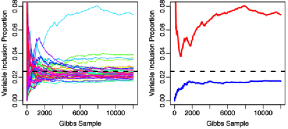
Figure 1: Variable inclusion proportions from BART model in null setting where each predictor variable is unrelated to the response variable. (Left) variable inclusion proportions for all $K=40$ predictor variables over 12,000 Gibbs samples. (Right) tracking of the maximum and minimum of the variable inclusion proportions.

In this setting, the variable inclusion proportions do not converge to $1/40=0.025$. As seen in Figure 1, some variable inclusion proportions remain substantially larger than $1/K$ and some are substantially smaller. We observed this same phenomenon with different levels of noise in the response variable.

3.3 Further exploration of null simulation

We hypothesize that the variation between $p_{k}$’s in Figure 1 can stem from two causes. First, even though the response and predictors were generated independently, they will still exhibit some random association. BART may be fitting noise, or “chance-capitalizing;” given its nonparametric flexibility, BART could be fitting to perceived nonlinear associations that are actually just noise. Second, there might be inherent variation in the BART estimation procedure itself, possibly due to the Gibbs sampler getting stuck in a local maximum.

Thus, we consider an experiment to explore the source of this variation among the $p_{k}$’s. We generate 100 data sets under the same setting as that in Figure 1. Within each data set, we run BART 50 times with different initial values for the model parameters randomly drawn from the respective prior distributions. Let $p_{ijk}$ denote the variable inclusion proportion for the $i$th data set, $j$th BART run, and the $k$th predictor variable. We then consider the decomposition into three nested variances listed in Table 1. Note that we use standard deviations in our illustration that follows.

Table 1: The three nested variances

$s^{2}_{ik}=\frac{1}{50}\sum_{j=1}^{50}(p_{ijk}-\bar{p}_{i\cdot k})^{2}$	The variability of BART estimation for a particular predictor
	$k$ in a particular data set $i$
$s^{2}_{k}=\frac{1}{100}\sum_{i=1}^{100}(\bar{p}_{i\cdot k}-\bar{p}_{\cdot\cdot k})^{2}$	The variability due to chance capitalization of the BART
	procedure for predictor $k$ across data sets
$s^{2}=\frac{1}{40}\sum_{k=1}^{40}(\bar{p}_{\cdot\cdot k}-\bar{p}_{\cdot\cdot\cdot})^{2}$	The variability across predictors

First consider what may happen if the source of Figure’s 1 observed pathology is purely due to BART’s Gibbs sampler getting stuck in different local posterior modes. On the first run for the first data set, BART would fall into a local mode where some predictors are naturally more important than others and, hence, the $p_{11k}$’s would be unequal. In the same data set, second run, BART might fall into a different local mode where the $p_{12k}$’s are unequal, but in a way that is different from the first run’s $p_{11k}$’s. This type of process would occur over all 50 runs. Thus, the $s_{1k}$, the standard deviation of $p_{ijk}$ over runs of BART on the first data set, would be large. Note that if there is no chance capitalization or overfitting, there should be no reason that averages of the proportions, the $\bar{p}_{1\cdot k}$’s, should be different from $1/K$ over repeated runs. Then, when the second data set is introduced, BART will continue to get stuck in different local posterior modes and the $s_{2k}$’s should be large, but the $\bar{p}_{2\cdot k}$’s should be near $1/K$. Hence, over all of the data sets, $\bar{p}_{i\cdot k}$’s should be approximately $1/K$, implying that the $s_{k}$’s should be small. In sum, BART getting stuck in local modes suggests large $s_{ik}$’s and small $s_{k}$’s.

Next consider what may happen if the source of Figure’s 1 observed pathology is purely due to BART chance-capitalizing on noise. On the first data set, over each run, BART does not get stuck in local modes and, therefore, the $p_{i1k}$’s across runs would be fairly stable. Hence, the $s_{1k}$’s would be small. However, in each of the runs, BART overfits in the same way for each data set. For example, perhaps BART perceives an association between $x_{1}$ and $y$ on the first data set. Hence, the $p_{1j1}$’s would be larger than $1/K$ on all restarts (BART would select $x_{1}$ as a splitting rule often due to the perceived association) and, thus, $\bar{p}_{1\cdot 1}>1/K$. Then, in the second data set, BART may perceive an association between $x_{3}$ and $y$, resulting in $p_{2j3}$’s being larger on all runs ($\bar{p}_{2\cdot 3}>1/K$). Thus, BART overfitting is indicated by small $s_{ik}$’s and large $s_{k}$’s.

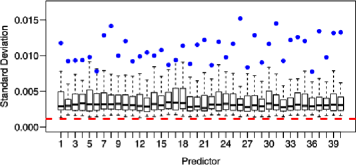
Figure 2: The boxplots represent the distribution of $s_{ik}$ for each predictor. The circles represent the values of $s_{k}$ and the dashed line corresponds to $s$. Note that the results are reported as standard deviations and points in the boxplots beyond the whiskers are omitted.

Figure 2 illustrates the results of the simulations. Both sources of variation appear, but for all predictors, the average $s_{ik}$ is significantly smaller than the $s_{k}$. This finding suggests that within a particular data set, BART is chance-capitalizing and overfitting to the noise, which prevents the $p_{k}$’s from converging to $1/K$.

Also note the overall average inclusion proportion $\bar{p}_{\cdot\cdot\cdot}$ is $0.025=1/K$, so across data sets and BART runs the variable inclusion proportions are correct on average. Further, the standard deviation across predictors $s$ is small. This implies that the $\bar{p}_{\cdot\cdot k}$’s are approximately $1/K$ as well, which indicates there is no systematic favoring of different covariates once the effect of overfitting by data set and remaining in local modes by run is averaged out.

We believe this experiment demonstrates that there is a large degree of chance capitalization present in the variable inclusion proportions in the “null” model. This implies that it is not possible to decide on an appropriate threshold for the $p_{k}$’s when selecting a subset of important predictor variables in real data settings. Further, the chance capitalization is idiosyncratic for any data set, making it challenging to pose a simple parametric model for the behavior in Figure 1 that would be useful in practice. This motivates our nonparametric approach to establishing thresholds for the variable inclusion proportions based on permutations of the response variable $\mathbf{y}$.

As noted above, there is some variability in the $p_{k}$’s between BART runs from different starting points. We found that averaging over results from five repetitions of the BART algorithm from different starting points was sufficient to provide stable estimates of the variable inclusion proportions and use these averaged values as our variable inclusion proportions for the remainder of the article.

3.4 Variable inclusion proportions under permuted responses

We now address our key question: how large does the variable inclusion frequency $p_{k}$ have to be in order to select predictor variable $\mathbf{x}_{k}$? To determine an appropriate selection threshold, we employ a permutation-based approach to generate a null distribution for the variable inclusion proportions $\mathbf{p}=(p_{1},\ldots,p_{K})$.

Specifically, we create $P$ permutations of the response vector: $\mathbf{y}^{*}_{1},\mathbf{y}^{*}_{2},\ldots,\mathbf{y}^{*}_{P}$. For each of these permuted response vectors $\mathbf{y}^{*}_{p}$, we run the BART model using $\mathbf{y}^{*}_{p}$ as the response and the original $\mathbf{x}_{1},\ldots,\mathbf{x}_{K}$ as predictor variables. This permutation strategy preserves possible dependencies among the predictor variables while removing any dependency between the predictor variables and the response variable.

We retain the variable inclusion proportions estimated from the BART run using each permuted response $\mathbf{y}^{*}_{p}$. We use the notation $p^{*}_{k,p}$ for the variable inclusion proportion from BART for predictor $\mathbf{x}_{k}$ from the $p$th permuted response, and we use the notation $\mathbf{p}^{*}_{p}$ for the vector of all variable inclusion proportions from the $p$th permuted response. We use the variable inclusion proportions $\mathbf{p}^{*}_{1},\mathbf{p}^{*}_{2},\ldots,\mathbf{p}^{*}_{P}$ across all $P$ permutations as the null distribution for our variable inclusion proportions $\mathbf{p}$ from the real (unpermuted) response $\mathbf{y}$.

The remaining issue is selecting an appropriate threshold for predictor $\mathbf{x}_{k}$ based on the permutation null distribution $\mathbf{p}^{*}_{1},\mathbf{p}^{*}_{2},\ldots,\mathbf{p}^{*}_{P}$. We will consider three different threshold strategies that vary in terms of the stringency of their resulting variable selection procedure.

The first strategy is a “local” threshold: we calculate a threshold for each variable inclusion proportion $p_{k}$ for each predictor $\mathbf{x}_{k}$ based only on the permutation null distribution of $p_{k}$. Specifically, we take the $1-\alpha$ quantile of the distribution of $p^{*}_{k,1},p^{*}_{k,2},\ldots,p^{*}_{k,P}$ and only select predictor $\mathbf{x}_{k}$ if $p_{k}$ exceeds this $1-\alpha$ quantile.

The second strategy is a “global max” threshold: we calculate a threshold for the variable inclusion proportion $p_{k}$ for predictor $\mathbf{x}_{k}$ based on the maximum across the permutation distributions of the variable inclusion proportions for all predictor variables. Specifically, we first calculate $p^{*}_{\max,p}=\max\{p^{*}_{1,p},p^{*}_{2,p},\ldots,p^{*}_{K,p}\}$, the largest variable inclusion proportion across all predictor variables in permutation $p$. We then calculate the $1-\alpha$ quantile of the distribution of $p^{*}_{\max,1},p^{*}_{\max,2},\ldots,p^{*}_{\max,P}$ and only select predictor $\mathbf{x}_{k}$ if $p_{k}$ exceeds this $1-\alpha$ quantile.

The first “local” strategy and the second “global max” strategy are opposite extremes in terms of the stringency of the resulting variable selection. The local strategy is least stringent since the variable inclusion proportion $p_{k}$ for predictor $\mathbf{x}_{k}$ needs to only be extreme within its own permutation distribution in order to be selected. The global maximum strategy is most stringent since the variable inclusion proportion $p_{k}$ for predictor $\mathbf{x}_{k}$ must be extreme relative to the permutation distribution across all predictor variables in order to be selected.

We consider a third strategy that is also global across predictor variables, but is less stringent than the global max strategy. The third “global SE” strategy uses the mean and standard deviation from the permutation distribution of each variable inclusion proportion $p_{k}$ to create a global threshold for all predictor variables. Specifically, letting $m_{k}$ and $s_{k}$ be the mean and standard deviation of variable inclusion proportion $p^{*}_{k}$ for predictor $\mathbf{x}_{k}$ across all permutations, we calculate

$$C^{*}=\inf_{C\in\mathbb{R}^{+}}\Biggl{\{}\forall k,\frac{1}{P}\sum_{p=1}^{P}\mathbb{I}\bigl{(}p^{*}_{k,p}\leq m_{k}+C\cdot s_{k}\bigr{)}>1-\alpha\Biggr{\}}.$$

The value $C^{*}$ is the smallest global multiplier that gives simultaneous $1-\alpha$ coverage across the permutation distributions of $p_{k}$ for all predictor variables. The predictor $\mathbf{x}_{k}$ is then only selected if $p_{k}>m_{k}+C^{*}\cdot s_{k}$. This third strategy is a compromise between the local permutation distribution for variable $k$ (by incorporating each mean $m_{k}$ and standard deviation $s_{k}$) and the global permutation distributions of the other predictor variables (through $C^{*}$). We outline all three thresholding procedures in more detail in the Appendix.

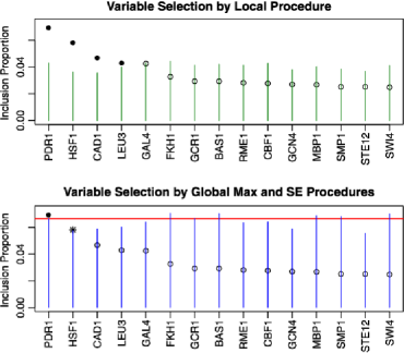
Figure 3: The fifteen largest variable inclusion proportions from BART implemented on the yeast gene YAL004W with $\alpha=0.05$. (Top) the tips of the green bands are the “local” thresholds of our first variable selection strategy. Solid dots are selected predictor variables, whereas hollow dots are unselected predictor variables. (Bottom) the red line is the threshold from our second “global max” strategy. The tips of the blue bands are the thresholds from our “global SE” strategy. The one solid dot is the predictor selected by both strategies. The star is the additional predictor variable selected by only the global SE strategy. The hollow dots are unselected predictor variables.

As an example of these three thresholding strategies, we provide a brief preview of our application to the yeast gene regulatory network in Section 5. In that application, the response variable $\mathbf{y}$ consists of the expression measures for a particular gene across approximately 300 conditions and the predictor variables are the expression values for approximately 40 transcription factors in those same 300 conditions.

In Figure 3, we give the fifteen predictor variables with the largest variable inclusion proportions from the BART model implemented on the data for a particular yeast gene YAL004W. In the top plot, we see the different “local” thresholds for each predictor variable. Four of the predictor variables had variable inclusion proportions $p_{k}$ that exceeded their local threshold and were selected under this first strategy. In the bottom plot, we see the single “global max” threshold for all predictor variables as well as the different “global SE” thresholds for each predictor variable. Two of the predictor variables had variable inclusion proportions $p_{k}$ that exceeded their global SE thresholds, whereas only one predictor variable exceeded the global max threshold.

This example illustrates that our three threshold strategies can differ substantially in terms of the stringency of the resulting variable selection. Depending on our prior expectations about the sparsity in our predictor variables, we may prefer the high stringency of the global max strategy, the low stringency of the local strategy, or the intermediary global SE strategy.

In practice, it may be difficult to know a priori the level of stringency that is desired for a real data application. Thus, we propose a cross-validation strategy for deciding between our three thresholding strategies for variable selection. Using $k$-fold cross-validation, the available observations can be partitioned into training and holdout subsets. For each partition, we can implement all three thresholding strategies on the training subset of the data and use the thresholding strategy with the smallest prediction error across the holdout subsets. We call this procedure “BART-Best” and provide implementation details in the Appendix.

Our permutation-based approach for variable selection does not require any additional assumptions beyond those of the BART model. Once again, the sum-of-trees plus normal errors is a flexible assumption that should perform well across a wide range of data settings, especially relative to methods that make stronger parametric demands. Also, it is important to note that we view each of the strategies described in this section as a procedure for variable selection based on well-founded statistical principles, but do not actually associate any particular formal hypothesis testing with our approach. Finally, a disadvantage of our permutation-based proposal is the computational cost of running BART on a large set of permuted response variables $\mathbf{y}^{*}$. However, it should be noted that the permuted response vector runs can be computed in parallel on multiple cores when such resources are available.

3.5 Real prior information in BART-based variable selection

Most variable selection approaches do not allow for a priori preferences for particular predictor variables. However, in many applications, there may be available prior information that suggests particular predictor variables may be more valuable than others.

As an example, the yeast regulatory data in Section 5 consist of expression measures $\mathbf{y}_{g}$ for a particular gene $g$ as the response variable with predictor variables $\mathbf{x}_{k}$ being the expression values for $\approx$40 transcription factors. In addition to the expression data, we also have an accompanying ChIP-binding data set [Lee et al. (2002)] that indicates for each gene $g$ which of the $\approx$40 transcription factors are likely to bind near that gene. We can view these ChIP-binding measures as prior probabilities that particular predictor variables $\mathbf{x}_{k}$ will be important for the response variable $\mathbf{y}$.

The most natural way to give prior preference to particular variables in BART is to alter the prior on the splitting rules. As mentioned in Section 3.1, by default each predictor $\mathbf{x}_{k}$ has an equal a priori chance of being chosen as a splitting rule for each tree branch in the BART ensemble. We propose altering the prior of the standard BART implementation so that when randomly selecting a particular predictor variable for a splitting rule, more weight is given to the predictor variables that have a higher prior probability of being important. Additionally, the prior on the tree structure, which is needed for the Metropolis–Hastings ratio computation, is appropriately adjusted. This strategy has some precedent, as Chipman, George and McCulloch (1998) discuss nonuniform criteria for splitting rules in the context of an earlier Bayesian Classification and Regression Tree implementation. Note that when employing one of the strategies discussed in Section 3.4, the prior is reset to discrete uniform when generating the permutation distribution, as it is assumed that there is no relationship between the predictors and the response.

In Section 4.3 we present a simulation-based evaluation of the effects on correct variable selection when an informed prior distribution is either correctly specified, giving additional weight to the predictor variables with true influence on the response, or incorrectly specified, giving additional weight to predictor variables that are unrelated to the response. Before our simulation study of the effects of prior information, we first present an extensive simulation study that compares our BART-based variable selection procedure to several other approaches.

4 Simulation evaluation of BART-based variable selection

We use a variety of simulated data settings to evaluate the ability of our BART-based procedure to select the subset of predictor variables that have a true influence on a response variable. We examine settings where the response is a linear function of the predictor variables in Section 4.1 as well as settings where the response is a nonlinear function of the predictor variables in Section 4.2. We also examine the effects of correctly versus incorrectly specified informed prior distributions in Section 4.3. For each simulated data setting, we will compare the performance of several different variable selection approaches:

[(1)]

BART-based variable selection: As outlined in Section 3, we use the variable inclusion proportions from BART to rank and select predictor variables. We will evaluate the performance of the three proposed thresholding strategies as well as “BART-Best,” the (five-fold) cross-validation strategy for choosing among our thresholding strategies. In each case, we set $\alpha=0.05$ and the number of trees $m$ is set to 20. Default settings from Chipman, George and McCulloch (2010) are used for all other hyperparameters. The variable selection procedures are implemented in the R package bartMachine [Kapelner and Bleich (2014)].

Stepwise regression: Backward stepwise regression using the stepAIC function in R.

Lasso regression: Regression with a lasso (L1) penalty can be used for variable selection by selecting the subset of variables with nonzero coefficient estimates. For this procedure, an additional penalty parameter $\lambda$ must be specified, which controls the amount of shrinkage toward zero in the coefficients. We use the glmnet package in R [Friedman, Hastie and Tibshirani (2010)], which uses ten-fold cross-validation to select the value of the penalty parameter $\lambda$.

Random forests (RF): Similarly to BART, RF must be adapted to the task of variable selection. The randomForest package in R [Liaw and Wiener (2002)] produces an “importance score” for each predictor variable: the change in out-of-bag mean square error when that predictor is not allowed to contribute to the model. Breiman and Cutler (2013) suggest selecting only variables where the importance score exceeds the $1-\alpha$ quantile of a standard normal distribution. We follow their approach and further suggest a new approach: using the Bonferroni-corrected $(1-\alpha)/p$ quantile of a standard normal distribution. We employ a five-fold cross-validation approach to pick the best of these two thresholding strategies in each simulated data setting and let $\alpha=0.05$. Default parameter settings for RF are used.

Dynamic trees (DT): Gramacy, Taddy and Wild (2013) introduce a backward variable selection procedure for DT. For each predictor, the authors compute the average reduction in posterior predictive uncertainty across all nodes using the given predictor as a splitting variable. The authors then propose a relevance probability, which is the proportion of posterior samples in which the reduction in predictive uncertainty is positive. Variables are deselected if their relevance probability does not exceed a certain threshold. After removing variables, the procedure is repeated until the log-Bayes factor of the larger model over the smaller model is positive, suggesting a preference for the larger model. We construct DT using the R package dynaTree [Taddy, Gramacy and Polson (2011)] with 5000 particles and a constant leaf model. We employ the default relevance threshold suggested by the authors of 0.50.

Spike-and-slab regression (Spike-slab): We employ the spike-and-slab regression procedure outlined in Ishwaran and Rao (2005) and Ishwaran and Rao (2005). The procedure first fits a spike-and-slab regression model and then performs variable selection via the generalized elastic net. Variables with nonzero coefficients are considered relevant. The method is applicable to both high- and low-dimensional problems, as in the high-dimensional setting, a filtering of the variables is first performed for dimension reduction. The procedure is implemented in the R package Spikeslab [Ishwaran, Rao and Kogalur (2013)].

Each of the above methods will be compared on the ability to select “useful” predictor variables, the subset of predictor variables that truly affect the response variable. We can quantify this performance by tabulating the number of true positive (TP) selections, false positive (FP) selections, true negative (TN) selections, and false negative (FN) selections. The precision of a variable selection method is the proportion of truly useful variables among all predictor variables that are selected,

$$\mathrm{Precision}=\frac{\mathrm{TP}}{\mathrm{TP}+{\mathrm{FP}}}.$$ (2)

The recall of a variable selection method is the proportion of truly useful variables selected among all truly useful predictor variables,

$$\mathrm{Recall}=\frac{\mathrm{TP}}{\mathrm{TP}+\mathrm{FN}}.$$ (3)

We can combine the precision and recall together into a single performance criterion,

$$F_{1}=2\cdot\frac{\mathrm{Precision}\cdot\mathrm{Recall}}{\mathrm{Precision}+\mathrm{Recall}},$$ (4)

which is the harmonic mean of precision and recall, balancing a procedure’s capability to make necessary identifications with its ability to avoid including irrelevant predictors. This $F_{1}$ measure is called the “effectiveness” by van Rijsbergen (1979) and is used routinely in information retrieval and categorization problems.

While many variable selection simulations found in the literature rely on out-of-sample root mean square error (RMSE) to assess performance of a procedure, we believe the $F_{1}$ score is a better alternative. Out-of-sample RMSE inherently overweights recall vis-à-vis precision since predictive performance depends more heavily on including covariates which generate signal. This is especially true for adaptive learning algorithms.

We chose the balanced $F_{1}$ metric because we want to demonstrate flexible performance while balancing both recall and precision. For example, if an investigator is searching for harmful physiological agents that can affect health outcomes, identifying the complete set of agents is important (recall). If the investigator is looking to fund new, potentially expensive research based on discoveries (as in our application in Section 5), avoiding fruitless directions is most important (precision).

4.1 Simulation setting 1: Linear relationship

We first examine the performance of the various variable selection approaches in a situation where the response variable is a linear function of the predictor variables. Specifically, we generate each predictor vector $\mathbf{x}_{j}$ from a normal distribution

$$\mathbf{x}_{1},\ldots,\mathbf{x}_{p}\stackrel{{\scriptstyle\mathrm{i.i.d.}}}{{\sim}}\mathcal{N}_{n}(\mathbf{0},\mathbf{I}),$$ (5)

and then the response variable $\mathbf{y}$ is generated as

$$\mathbf{y}=\mathbf{X}\bolds{\beta}+\bolds{\mathcal{E}},\qquad\bolds{\mathcal{E}}\sim\mathcal{N}_{n}\bigl{(}\mathbf{0},\sigma^{2}\mathbf{I}\bigr{)},$$ (6)

where $\bolds{\beta}=[\mathbf{1}_{p_{0}},\mathbf{0}_{p-p_{0}}]^{\top}$. In other words, there are $p_{0}$ predictor variables that are truly related to the response $\mathbf{y}$, and $p-p_{0}$ predictor variables that are spurious. The sparsity of a particular data setting is reflected in the proportion $p_{0}/p$ of predictor variables that actually influence the response.

Fifty data sets were generated for each possible combination of the following different parameter settings: $p\in{}${20, 100, 200, 500, 1000}, $p_{0}/p\in{}${0.01, 0.05, 0.1, 0.2} and $\sigma^{2}\in{}${1, 5, 20}. In each of the 60 possible settings, the sample size was fixed at $n=250$.

Figure 4 gives the $F_{1}$ performance measure for each variable selection method for 8 of the 60 simulation settings. We have chosen to illustrate these simulation results, as they are representative of our overall findings. Here, higher values of $F_{1}$ indicate better performance. Complete tables of precision, recall, and $F_{1}$ measure values for the simulations shown in Figure 4 can be found in the supplementary materials [Bleich et al. (2014)].

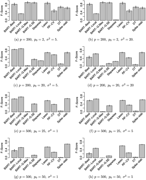
Figure 4: Average $F_{1}$ measures for different variable selection approaches on simulated data under the linear model setting across 50 simulations. The black bars represent 90% error bars for the average. Results for $p=200$ and $p=500$ are shown. Within each choice of $p$, moving down a column shifts from high to low sparsity and moving across a row shifts from low to high noise.

We first focus on the comparisons in performance between the four thresholding strategies for our BART-based variable selection procedure: our three thresholding strategies plus the BART-Best cross-validated threshold strategy. First, we consider the case where $p=200$. In the more sparse settings [Figure 4(a) and (b)], the more stringent global max and global SE strategies perform better than the less stringent local thresholding strategy. However, the local thresholding strategy performs better in the less sparse settings [Figure 4(c) and (d)]. The BART-Best procedure with a cross-validated threshold performs slightly worse than the best of the three thresholds in each setting, but fares quite well uniformly. Hence, the cross-validated threshold strategy represents a good choice when the level of sparsity is not known a priori.

For the settings where $p=500$, the findings are relatively similar. The local thresholding strategy performs well given the fact that the data is less sparse. Performance also degrades when moving from the low noise settings [Figure 4(e) and (f)] to the high noise settings [Figure 4(g) and (h)]. Note that BART-Best does not perform particularly well in Figure 4(h).

Comparing with the alternative approaches when $p=200$, we see that BART-Best performs better than all of the alternatives in the lower noise, more sparse setting [Figure 4(a)] and is competitive with the lasso in the lower noise, less sparse setting [Figure 4(c)]. BART-Best is competitive with the lasso in the higher noise, more sparse setting [Figure 4(b)] and beaten by the linear methods in the higher noise, less sparse setting [Figure 4(d)]. When $p=500$, the cross-validated BART is competitive with the lasso and Spike-slab and outperforms the nonlinear methods when $p_{0}=25$ [Figure 4(e) and (f)]. When $p_{0}=50$ [Figure 4(g) and (h)], the cross-validated BART performs worse than the lasso and Spike-slab, and has performance on par with the cross-validated RF.

Overall, the competitive performance of our BART-based approach is especially impressive since BART does not assume a linear relationship between the response and predictor variables. One would expect that stepwise regression, lasso regression, and Spike-slab would have an advantage since these methods assume a linear model which matches the data generating process in this setting. Like BART, RF and DT also do not assume a linear model, but in most of the cases we examined, our BART-based variable selection procedure performs better than RF and DT. We note that DT does not perform well on this simulation, possibly suggesting the need for a cross-validation procedure to choose appropriate relevance thresholds in different data settings.

Additionally, we briefly address the computational aspect of our four proposed approaches here by giving an estimate of the runtimes. For this data with $n=250$ and $p=200$, the three strategies (local, global max, and global SE) are estimated together in one bartMachine function in about 90 seconds. The cross-validated BART-Best procedure takes about 7 minutes.

4.2 Simulation setting 2: Nonlinear relationship

We next examine the performance of the variable selection methods in a situation where the response variable is a nonlinear function of the predictor variables. Specifically, we generate each predictor vector $\mathbf{x}_{j}$ from a uniform distribution,

$$\mathbf{x}_{1},\ldots,\mathbf{x}_{p}\stackrel{{\scriptstyle\mathrm{i.i.d.}}}{{\sim}}\mathrm{U}_{n}(0,1),$$

and then the response variable $\mathbf{y}$ is generated as

$$\mathbf{y} = 10\sin{\pi\mathbf{x}_{1}\mathbf{x}_{2}}+20(\mathbf{x}_{3}-0.5)^{2}+10\mathbf{x}_{4}+5\mathbf{x}_{5}+\bolds{\mathcal{E}},$$

$$\eqntext{\bolds{\mathcal{E}}\sim\mathcal{N}_{n}\bigl{(}\mathbf{0},\sigma^{2}\mathbf{I}\bigr{)}.}$$ (8)

This nonlinear function from Friedman (1991), used to showcase BART in Chipman, George and McCulloch (2010), is challenging for variable selection models due to its interactions and nonlinearities. In this data setting, only the first five predictors truly influence the response, while any additional predictor variables are spurious.

Fifty data sets were generated for each possible combination of $\sigma^{2}\in{}${5, 100, 625} and $p\in{}${25, 100, 200, 500, 1000}. Since the number of relevant predictor variables is fixed at five, we simulate over a wide range of sparsity values ranging from $p_{0}/p=0.2$ down to $p_{0}/p=0.005$. In each data set, the sample size was fixed at $n=250$.

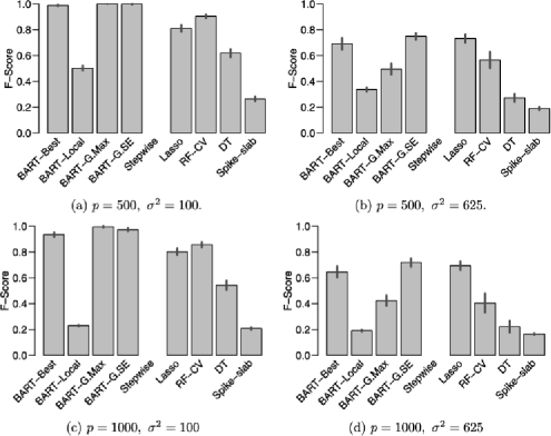
Figure 5: Average $F_{1}$ measures across 50 simulations for different variable selection approaches on simulated data under the Friedman model setting. The black bars represent 90% error bars for the average. Moving from the top row to the bottom shifts from low to high dimensionality and moving from the left column to the right shifts from low to high noise.

Figure 5 illustrates the $F_{1}$ performance measure for each variable selection method for four of the $(p,\sigma^{2})$ simulation pairs. We have chosen to illustrate these simulation results, as they are representative of our overall findings. Backward stepwise regression via stepAIC could not be run in these settings where $n<p$ and is excluded from these comparisons (values in Figure 5 for this procedure are set to 0). Complete tables of precision, recall, and $F_{1}$ measure values for the simulations shown in Figure 5 are given in our supplementary materials [Bleich et al. (2014)].

Just comparing the four thresholding strategies of our BART-based procedure, we see that the more stringent selection criteria have better $F_{1}$ performance measures in all of these sparse cases. The cross-validated threshold version of our BART procedure performs about as well as the best individual threshold in each case.

Compared to the other variable selection procedures, the cross-validated BART-Best has the strongest overall performance. Our cross-validated procedure outperforms DT and RF-CV in all situations. The assumption of linearity puts the lasso and Spike-slab at a disadvantage in this nonlinear setting. Spike-slab does not perform well on this data, although lasso performs well. BART-Best and the cross-validated RF have the best performance in the low noise settings [Figure 5(a) and (c)], as they do not assume linearity. Moving to the high noise settings [Figure 5(b) and (d)], BART and RF both see a degradation in performance, and BART-Best and the lasso are the best performers, followed by the cross-validated RF.

4.3 Simulation setting 3: Linear model with informed priors

In the next set of simulations, we explore the impact of incorporating informed priors into the BART model, as discussed in Section 3.5. We will evaluate the performance of our BART-based variable selection procedure in cases where the prior information is correctly specified as well as in cases where the prior information is incorrectly specified.

We will use the linear model in Section 4.1 as our data generating process. We will consider a specific case of the scheme outlined in Section 3.5 where particular subsets of predictor variables are given twice as much weight as the rest of the predictor variables. With a noninformative prior, each predictor variable has a probability of $1/p$ of being selected as the splitting variable for a splitting rule. For the informed prior, a subset of $p_{0}$ predictor variables is given twice as much weight, which gives those variables a larger probability of $2/(p+p_{0})$ of being selected as a splitting variable.

For the fifty data sets generated under each combination of the parameter settings in the simulations of Section 4.1, we implemented three different versions of BART: (1) BART with a noninformative prior on the predictor variables, (2) BART with a “correctly” informed prior (twice the weight on the subset of predictor variables that have a true effect on response), and (3) BART with an “incorrectly” informed prior (twice the weight on a random subset of spurious predictor variables). For each of these BART models, predictor variables were then selected using the cross-validated threshold strategy.

Figure 6 gives the $F_{1}$ measures for the three different BART priors in four of the data settings outlined in Section 4.1.

Figure 6: Average $F_{1}$ measures across 50 simulations for BART-based variable selection under three different prior choices. The black bars represent 90% error bars for the average. The settings shown are the same as those in Figure 4(a)–(d).

There are two key observations from the results in Figure 6. First, correct prior information can substantially benefit the variable selection ability of our BART adaptation, especially in higher noise settings [Figure 6(b) and (d)]. Second, incorrect prior information does not degrade performance in any of the cases, which suggests that our BART-based variable selection procedure is robust to the misspecification of an informed prior on the predictor variables. This seems to be a consequence of the Metropolis–Hastings step, which tends to not accept splitting rules that substantially reduce the model’s posterior value, regardless of how often they are proposed.

To summarize our simulation studies in Section 4, our BART-based variable selection procedure is competitive with alternative approaches when there is a linear relationship between the predictor variables and the response, and performs better than alternative approaches in a nonlinear data setting. BART-based variable selection can be further improved by correctly specifying prior information (when available) that gives preference to particular predictor variables and appears to be robust to misspecification of this prior information.

5 Application to gene regulation in yeast

Experimental advances in molecular biology have led to the availability of high-dimensional genomic data in a variety of biological applications. We will apply our BART-based variable selection methodology to infer the gene regulatory network in budding yeast (Saccharomyces cerevisiae). One of the primary mechanisms by which genes are regulated is through the action of transcription factors, which are proteins that increase or decrease the expression of a specific set of genes.

The data for our analyses are expression measures for 6026 genes in yeast across 314 experiments. For those same 314 experiments, we also have expression measures for 39 known transcription factors. For each of the 6026 genes, our goal is to identify the subset of the 39 transcription factors that have a real regulatory relationship with that particular gene.

We consider each of the 6026 genes as a separate variable selection problem. For a particular gene $g$, we model the expression measures for that gene as a $314\times 1$ response vector $\mathbf{y}_{g}$ and we have 39 predictor variables ($\mathbf{x}_{1},\ldots,\mathbf{x}_{39}$) which are the expression measures of each of the 39 transcription factors. This same data was previously analyzed using a linear regression approach in Jensen, Chen and Stoeckert (2007), but we will avoid assumptions of linearity by employing our BART-based variable selection procedure.

We also have additional data available for this problem that can be used as prior information on our predictor variables. Lee et al. (2002) performed chromatin immunoprecipitation (ChIP) experiments for each of the 39 transcription factors that we are using as predictor variables. The outcome of these experiments is the estimated probabilities $m_{gk}$ that gene $g$ is physically bound by each transcription factor $k$. Guang, Jensen and Stoeckert (2007) give details on how these probabilities $m_{gk}$ are derived from the ChIP data.

We will incorporate these estimated probabilities into our BART-based variable selection approach as prior information. When selecting predictor variables for splitting rules, we give more weight to the transcription factors $k$ with larger prior probabilities $m_{gk}$ in the BART model for gene $g$. Specifically, we have a splitting variable weight $w_{gk}$ for predictor $\mathbf{x}_{k}$ in the BART model for gene $g$, which we calculate as

$$w_{gk}=1+c\cdot m_{gk}.$$ (9)

In the BART model for gene $g$, each predictor $\mathbf{x}_{k}$ is chosen for a splitting rule with probability proportional to $w_{gk}$. The global parameter $c$ controls how influential the informed prior probabilities $m_{gk}$ are on the splitting rules in BART. Setting $c=0$ reduces our informed prior to the uniform splitting rules of the standard BART implementation. Larger values of $c$ increase the weights of predictor variables with large prior probabilities $m_{gk}$, giving the informed prior extra influence.

In a real data setting such as our yeast application, it is difficult to know how much influence to give our informed priors on the predictor variables. We will consider several different values of $c={}${0, 1, 2, 4, 10,000} and choose the value that results in the smallest prediction error on a subset of the observed data that is held out from our BART model estimation. Specifically, recall that we have 314 expression measures for each gene in our data set. For each gene, we randomly partition these observations into an 80% training set, 10% tuning set, and 10% hold-out set. For each value of $c={}${0, 1, 2, 4, 10,000}, we fit a BART model on the 80% training set and then choose the value of $c$ that gives the smallest prediction error on the 10% tuning set. This same 10% tuning set is also used to choose the best threshold procedure among the three options outlined in Section 3.4. We will use the terminology “BART-Best” to refer to the BART-based variable selection procedure that is validated over the choice of $c$ and the three thresholding strategies. While we could also cross-validate over the significance level $\alpha$, we fix $\alpha=0.05$ due to computational concerns given the large number of data sets to be analyzed.

For each gene, we evaluate our approach by refitting BART using only the variables selected by our BART-based variable selection model and evaluate the prediction accuracy on the final 10% hold-out set of data for that gene. This same 10% hold-out set of data for each gene is also used to evaluate the prediction accuracy of various alternative variable selection methods. We consider the alternative methods of stepwise regression, lasso regression, RF, DT, and Spike-slab in similar fashions to Section 4. The 10% tuning set is used to choose the value of the penalty parameter $\lambda$ for lasso regression as well as the importance score threshold for RF. For DT, we use a constant leaf model for variable selection and then construct a linear leaf model using the selected variables for prediction.

We also consider three simpler approaches that do not select particular predictor variables: (1) “BART-Full” which is the BART model using all variables, (2) ordinary least squares regression (OLS) with all predictor variables included, and (3) the “null” model: the sample average of the response which does not make use of any predictors. In the null model, we do include an intercept, so we are predicting for the hold-out set of expression measures for each gene with the average expression level of that gene in the training set.

We first examined the distribution of RMSEs across the 6026 genes. We found that each procedure improves over the null model with no covariates, suggesting that some subset of transcription factors is predictive of gene expression for most of the 6026 genes. However, for a minority of genes, the null model is competitive, suggesting that the 39 available transcription factors may not be biologically relevant to every one of these genes. The nonnull variable selection methods show generally similar performance in terms of the distribution of RMSEs, and a corresponding figure can be found in the supplementary materials [Bleich et al. (2014)]. It is important to note that predictive accuracy in the form of out-of-sample RMSE is not the most desirable metric for comparing variable selection techniques because it overweights recall relative to precision.

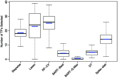
Figure 7: Distributions of the number of predictor variables selected for each method across all 6026 genes. Blue bars represent the average number of selected predictor variables. Not shown are the null model which uses no predictors as well as OLS and the full BART model which both use all predictors. Points beyond the whiskers are omitted.

In Figure 7, we show the distribution of the number of selected predictor variables (TFs) across the 6026 genes, where we see substantial differences between the variable selection procedures. Figure 7 confirms that BART-G.max is selecting very few TFs for each gene. Even more interesting is the comparison of BART-Best to stepwise regression, lasso regression, RF, and Spike-slab. BART-Best is selecting far fewer TFs than these alternative procedures. Interestingly, DT, the other Bayesian tree-based algorithm, selects a number of TFs most comparable to BART-Best.

Given the relatively similar performance of methods in terms of RMSE and the more substantial differences in number of variables selected, we propose the following combined measure of performance for each variable selection method:

$$(\mbox{RMSE reduction per predictor})_{\mathrm{method}}=\frac{\mathrm{RMSE}_{\mathrm{null}}-\mathrm{RMSE}_{\mathrm{method}}}{\mathrm{NumPred}_{\mathrm{method}}},$$

where $\mathrm{RMSE}_{\mathrm{method}}$ and $\mathrm{NumPred}_{\mathrm{method}}$ are, respectively, the out-of-sample RMSE and number of predictors selected for a particular method. This performance metric answers the question: how much “gain” are we getting for adding each predictor variable suggested by a variable selection approach? Methods that give larger RMSE reduction per predictor variable are preferred.

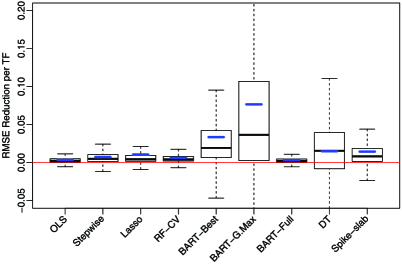
Figure 8: Distributions of the RMSE reduction per predictor for each method across all 6026 genes. Blue bars represent the average RMSE reduction per predictor. Points beyond the whiskers are omitted.

Figure 8 gives the RMSE reduction per predictor for each of our variable selection procedures. Note that we only plot cases where at least one predictor variable is selected, since RMSE reduction per predictor is only defined if the number of predictors selected is greater than zero.

Our BART-Best variable selection procedure gives generally larger (better) values of the RMSE reduction per predictor measure than stepwise regression, lasso regression, RF, and Spike-slab. DT is the closer competitor, but does slightly worse, on average, than BART-Best. Also, both the BART-Full and OLS procedures, where no variable selection is performed, perform worse than the variable selection procedures.

BART-G.max, the BART-based procedure under the global max threshold, seems to perform even better than the BART-Best procedure in terms of the RMSE reduction per predictor measure. However, recall that we are plotting only cases where at least one predictor was selected. BART-G.max selects at least one transcription factor for only 2866 of the 6026 genes, though it shows the best RMSE reduction per predictor in these cases. By comparison, BART-Best selects at least one transcription for 5459 of the 6026 genes while showing better RMSE reduction per predictor than the non-BART variable selection procedures.

Additionally, Table 2 shows the proportion of times each choice of prior influence $c$ appeared in the “BART-Best” model. Almost a quarter of the time, the prior information was not used. However, there is also a large number of genes for which the prior was considered to have useful information and was incorporated into the procedure.

=170pt $\bolds{c}$ value Percentage of genes 0000,0 23.3% 0000,0.5 16.1% 0000,1 15.4% 0000,2 14.9% 0000,4 14.6% 10,000 15.7%

Table 2: Distribution of prior influence values $c$ used across the 6026 genes

Jensen, Chen and Stoeckert (2007) also used the same gene expression data (and ChIP-based prior information) to infer gene–TF regulatory relationships. A direct model comparison between our BART-based procedures and their approach is difficult since Jensen, Chen and Stoeckert (2007) fit a simultaneous model across all genes, whereas our current BART-based analysis fits a predictive model for each gene separately. In both analyses, prior information for each gene–TF pairing from ChIP binding data [Lee et al. (2002)] was used. However, in Jensen, Chen and Stoeckert (2007) the prior information for a particular TF was given the same weight (relative to the likelihood) for each gene in the data set. In our analysis, each gene was analyzed separately and so the prior information for a particular TF can be weighted differently for each gene.

A result of this modeling difference is that the prior information appears to have been given less weight by our BART-based procedure across genes, as evidenced by the substantial proportion of genes in Table 2 that were given zero or low weight ($c=0$ or $c=0.5$). Since that prior information played the role in Jensen, Chen and Stoeckert (2007) of promoting sparsity, a consequence of that prior information being given less weight in our BART-based analysis is reduced promotion of sparsity.

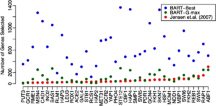
Figure 9: Number of genes for which each TF was selected. Results are compared for BART-Best, BART-G.Max, and the linear hierarchical model developed in Jensen, Chen and Stoeckert (2007).

This consequence is evident in Figure 9, where we compare the number of selected TFs. The $x$-axis gives the 39 transcription factors that served as the predictor variables for each of our 6026 genes. The $y$-axis is the number of genes for which that TF was selected as a predictor variable by each of three procedures: BART-Best, BART-G.max, and the analysis of Jensen, Chen and Stoeckert (2007). The most striking feature of Figure 9 is that each TF was selected for many more genes under our BART-Best procedure compared to BART-G.max, which also selected more variables than the analysis of Jensen, Chen and Stoeckert (2007). This result indicates that selecting more TFs per gene leads to the best out-of-sample predictive performance (i.e., BART-Best). It could be that Jensen, Chen and Stoeckert (2007) were over-enforcing sparsity, but that previous method also differed from our current approach in terms of assuming a linear relationship between the response and predictor variables.

6 Conclusion

Chipman, George and McCulloch’s (2010) Bayesian Additive Regression Trees is a rich and flexible model for estimating complicated relationships between a response variable and a potentially large set of predictor variables. We adapt BART to the task of variable selection by employing a permutation procedure to establish a null distribution for the variable inclusion proportion of each predictor. We present several thresholding strategies that reflect different beliefs about the degree of sparsity among the predictor variables, as well as a cross-validation procedure for choosing the best threshold when the degree of sparsity is not known a priori.

In contrast with popular variable selection methods such as stepwise regression and lasso regression, our BART-based approach does not make strong assumptions of linearity in the relationship between the response and predictors. We also provide a principled means to incorporate prior information about the relative importance of different predictor variables into our procedures.

We used several simulated data settings to compare our BART-based approach to alternative variable selection methods such as stepwise regression, lasso regression, random forests, and dynamic trees. Our variable selection procedures are competitive with these alternatives in the setting where there is a linear relationship between response and predictors, and performs better than these alternatives in a nonlinear setting. Additional simulation studies suggest that our procedures can be further improved by correctly specifying prior information (if such information is available) and seem to be robust when the prior information is incorrectly specified.

We applied our variable selection procedure, as well as alternative methods, to the task of selecting a subset of transcription factors that are relevant to the expression of individual genes in yeast (Saccharomyces cerevisiae). In this application, our BART-based variable selection procedure generally selected fewer predictor variables while achieving similar out-of-sample RMSE compared to the lasso and random forests. We combined these two observations into a single performance measure, RMSE reduction per predictor. In this application to inferring regulatory relationships in yeast, our BART-based variable selection demonstrates much better predictive performance than alternative methods such as lasso and random forests while selecting more transcription factors than the previous approach of Jensen, Chen and Stoeckert (2007).

While we found success using the variable inclusion proportions as the basis for our procedure, fruitful future work would be to explore the effect of a variance reduction metric, such as that explored in Gramacy, Taddy and Wild (2013) within BART.

Appendix: Pseudo-code for variable selection procedures

Procedure 1 Local threshold procedure

Compute $p_{1},\ldots,p_{K}$ $\triangleright$ Inclusion proportions from original data

for $i\leftarrow\{1,\ldots,P\}$ do $\triangleright$ $P$ is the number of null permutations

     $\mathbf{y^{*}}\leftarrow\mathrm{Permute}(\mathbf{y})$

     Run BART using $\mathbf{y^{*}}$ as response

     Compute $p_{i1}^{*},\ldots,p_{iK}^{*}$ $\triangleright$ Inclusion proportions from permuted data

end for

for $j\leftarrow\{1,\ldots,K\}$ do

     $q^{*}_{j}\leftarrow\operatorname{Quantile}(p^{*}_{1j},\ldots,p^{*}_{Pj},1-\alpha)$ $\triangleright$ $1-\alpha$ quantile of $\mathbf{x}_{j}$ permutation distribution

     if $p_{j}>q^{*}_{j}$ then Include $p_{j}$ in Vars end if

end for

return Vars

Procedure 2 Global maximum threshold procedure

Compute $p_{1},\ldots,p_{K}$ $\triangleright$ Inclusion proportions from original data

for $i\leftarrow\{1,\ldots,P\}$ do $\triangleright$ $P$ is the number of null permutations

     $\mathbf{y^{*}}\leftarrow\mathrm{Permute}(\mathbf{y})$

     Run BART using $\mathbf{y^{*}}$ as response

     Compute $p_{i1}^{*},\ldots,p_{iK}^{*}$ $\triangleright$ Inclusion proportions from permuted data

     $g_{i}\leftarrow\mathrm{Max}(p_{i1}^{*},\ldots,p_{iK}^{*})$ $\triangleright$ Maximum of proportions from permuted data

end for

$g^{*}\leftarrow\operatorname{Quantile}(g_{i},\ldots,g_{P},1-\alpha)$ $\triangleright$ $1-\alpha$ Quantile of maxima

for $j\leftarrow\{1,\ldots,K\}$ do

     if $p_{j}>g^{*}$ then Include $p_{j}$ in Vars end if

end for

return Vars

Procedure 3 Global standard error threshold procedure

Compute $p_{1},\ldots,p_{K}$ $\triangleright$ Inclusion proportions from original data

for $i\leftarrow\{1,\ldots,P\}$ do $\triangleright$ $P$ is the number of null permutations

     $\mathbf{y^{*}}\leftarrow\mathrm{Permute}(\mathbf{y})$

     Run BART using $\mathbf{y^{*}}$ as response

     Compute $p_{i1}^{*},\ldots,p_{iK}^{*}$ $\triangleright$ Inclusion proportions from permuted data

end for

for $j\leftarrow\{1,\ldots,K\}$ do

     $m_{j}\leftarrow\mathrm{Avg}(p^{*}_{1j},\ldots,p^{*}_{Pj})$ $\triangleright$ Sample average of $\mathbf{x}_{j}$ permutation distribution

     $s_{j}\leftarrow\mathrm{SD}(p^{*}_{1j},\ldots,p^{*}_{Pj})$ $\triangleright$ Sample sd of $\mathbf{x}_{j}$ permutation distribution

end for

$C^{*}\leftarrow\inf_{C\in\mathbb{R}^{+}}\{\forall j$, $\frac{1}{P}\sum_{i=1}^{P}\mathbb{I}(p^{*}_{ij}\leq m_{j}+C\cdot s_{j})>1-\alpha\}$ $\triangleright$ Simultaneous coverage

for $j\leftarrow\{1,\ldots,K\}$ do

     if $p_{j}>m_{j}+C^{*}\cdot s_{j}$ then Include $p_{j}$ in Vars end if

end for

return Vars

Procedure 4 Cross-Validated Comparison of Threshold Procedures

Divide the data into $K$ training-test splits

for $k\leftarrow\{1,\ldots,K\}$ do

     for method $\leftarrow\{$Local, Global Maximum, Global SE$\}$ do

         $\operatorname{Var}_{\mathrm{method}}\leftarrow$ Selected variables using method on BART

         $\mathrm{\texttt{BART}}_{\mathrm{method}}\leftarrow$ BART built from $k$th training set using only $\operatorname{Var}_{\mathrm{method}}$

         $L2_{k,\mathrm{method}}\leftarrow$ $L2$ error from $\mathrm{\texttt{BART}}_{\mathrm{method}}$ on $k$th test set

     end for

end for

for method $\leftarrow\{$Local, Global Maximum, Global SE$\}$ do

     $L2_{\mathrm{method}}\leftarrow\sum_{k=1}^{K}L2_{k,{\mathrm{method}}}$ $\triangleright$ Aggregate $L2$ error over entire training set

end for

method${}^{*}\leftarrow\arg\min_{\mathrm{method}}\{L2_{\mathrm{method}}\}$ $\triangleright$ Choose the best method from the three

return Selected variables using method^∗ for BART on full training set

References

- Bleich et al. (2014) {bmisc}[author] \bauthor\bsnmBleich, \binitsJ., \bauthor\bsnmKapelner, \binitsA., \bauthor\bsnmGeorge, \binitsE. and \bauthor\bsnmJensen, \binitsS. (\byear2014). \bhowpublishedSupplement to “Variable selection for BART: An application to gene regulation.” DOI:\doiurl10.1214/14-AOAS755SUPP. \bptokimsref \endbibitem
- Bottolo and Richardson (2010) {barticle}[mr] \bauthor\bsnmBottolo, \bfnmLeonard\binitsL. and \bauthor\bsnmRichardson, \bfnmSylvia\binitsS. (\byear2010). \btitleEvolutionary stochastic search for Bayesian model exploration. \bjournalBayesian Anal. \bvolume5 \bpages583–618. \biddoi=10.1214/10-BA523, issn=1936-0975, mr=2719668 \bptokimsref\endbibitem
- Breiman (2001) {barticle}[auto] \bauthor\bsnmBreiman, \bfnmL.\binitsL. (\byear2001). \btitleRandom forests. \bjournalMachine Learning \bvolume45 \bpages5–32. \bptokimsref\endbibitem
- Breiman and Cutler (2013) {bmisc}[auto:STB—2014/06/18—12:29:53] \bauthor\bsnmBreiman, \bfnmL.\binitsL. and \bauthor\bsnmCutler, \bfnmA.\binitsA. (\byear2013). \bhowpublishedOnline manual for random forests. Available at www.stat.berkeley.edu/~breiman/RandomForests/cc_home.htm. \bptokimsref\endbibitem