Proposed Method for Distinguishing Majorana Peak from Other Peaks: Tunneling Spectroscopy with Ohmic Dissipation using Resistive Electrodes

Abstract

We propose a scheme to distinguish zero-energy peaks due to Majorana from those due to other effects at finite temperature by simply replacing the normal metallic lead with a resistive lead (large $R\sim k\Omega$) in the tunneling spectroscopy. The dissipation effects due to the large resistance change the tunneling conductance significantly in different ways. The Majorana peak remains increase as temperature decreases $G\sim T^{2r-1}$ for $r=e^{2}R/h<1/2$. The zero-energy peak due to other effects splits into two peaks at finite temperature and the conductance at zero voltage bias varies with temperature by a power law. The dissipative tunneling with a Majorana mode belongs to a same universal class as the unstable critical point of the case with a non-Majorana mode.

Introduction — Majorana fermions (MFs), proposed to exist in solid state systems Fu and Kane (2008); Sau et al. (2010); Alicea (2010); Lutchyn et al. (2010); Oreg et al. (2010), cold atomic systems Sato et al. (2009); Zhu et al. (2011); Jiang et al. (2011a), and periodic driving systems Jiang et al. (2011a); Reynoso and Frustaglia (2013); Liu et al. (2013a), attract a great deal of attention. A variety of signatures Das Sarma et al. (2006); Fu and Kane (2009a, b); Akhmerov et al. (2009); Law et al. (2009); Akhmerov et al. (2011); M. et al. (2011); Liu and Baranger (2011); Jiang et al. (2011b); Fidkowski et al. (2012); San-Jose et al. (2012) are predicted to detect Majorana fermion (MF) zero mode; among them, tunneling spectroscopy may provide one of the simplest and direct tests for MF— The observation of the zero-bias peak (ZBP) with quantized conductance $G=2e^{2}/h$ Law et al. (2009); Akhmerov et al. (2011) at sufficiently low temperature (smaller than intrinsic width of the Majorana peak). Recently, several groups Mourik et al. (2012); Deng et al. (2012); Das et al. (2012) reported the observation of a non-quantized ZBP at higher temperature in semiconductor nanowires, which is possibly coming from MF. However, the ZBP may originate from other effects, e.g. zero-energy impurity bound state. In addition, recent works Bagrets and Altland (2012); Liu et al. (2012); Neven et al. (2013) show that, in a superconducting system with both spin-rotation and time-reversal symmetry breaking, the disorder can induce a cluster of mid-gap states around zero-energy and thus a ZBP at finite temperature. Especially, the disorder ZBP appears in the conditions highly similar to Majorana ZBP Bagrets and Altland (2012); Liu et al. (2012); Neven et al. (2013). These alternative possibilities lead to debates about the validity of the tunneling spectroscopy methods.

In this work, we introduce a scheme by simply replacing the normal metal lead in the tunneling spectroscopy with a resistive lead (with large resistance $R\sim k\Omega$). In this case, electrons couple to an ohmic environmental bath Feynman and Vernon (1963) in the tunneling process; the coupling to the bath usually suppresses the tunneling rate and leads to dissipative tunneling Leggett et al. (1987); Ingold and Yu.V. (1992). Dissipation effects can also cause non-trivial phase diagrams and transitions, which was recently observed in a simple resonant level system Mebrahtu et al. (2012, 2013); Liu et al. (2013b). We investigate how the dissipation influences the tunneling into MFs, zero-energy impurity bound states in superconductor, and other states causing ZBP at finite temperature. The ways that the dissipation effects renormalize the tunneling strength and the tunneling conductance is significantly different for MFs and other cases. If the lead is connected to a MF, the zero-bias conductance scales as $G\sim T^{2r-1}$ near a weak tunneling fixed point (high $T$) and will go to perfect transmission $G=2e^{2}/h$ at $T=0$ for $r=e^{2}R/h<1/2$. If the lead is connected to a superconductor (SC) with a zero-energy impurity bound state (non-MF), the system can be divided into four stable phases and an unstable symmetric point (i.e. critical point). Away from the symmetric point, the system will flow to one of the four stable fixed points, near which the zero-bias conductance scales as $G\sim T^{2r}$ and the peak splits into two at finite temperature. The critical point belongs to the same universal class as the case for dissipative tunneling into a Majorana mode. We also consider the conductance for the dissipative tunneling into a cluster of mid-gap states. Without dissipation, the finite temperature conductance shows ZBP; with dissipation, the single peak splits into two as temperature decreases. The splitting occurs at higher temperature for larger resistance, but $r<1/2$ is required in the experiment so that Majorana ZBP does not split. Therefore, the dissipation effect induced by the resistive lead provides a way to distinguish Majorana ZBP and other ZBP, and serves as a “ Majorana signature filter”.

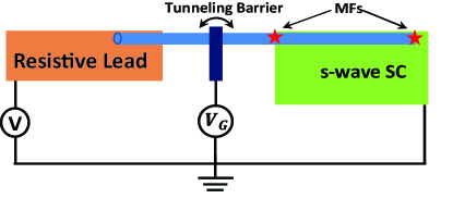
Figure 1: (color online) Proposed experimental setup.

Model — We consider the tunneling spectroscopy from a resistive lead into the end of a superconducting nanowire (SCNW) with Rashba spin-orbit coupling and proximity induced superconductivity $\Delta$ as shown in Fig. 1. A magnetic field is applied perpendicular to the direction of the Rashba spin-orbit coupling. In this case, MFs are predicted to exist at the two ends of the wire if $V_{z}>\sqrt{\Delta^{2}+\mu^{2}}$, where $V_{z}$ is Zeeman splitting and $\mu$ is wire chemical potential Lutchyn et al. (2010); Oreg et al. (2010). Unlike conventional setup, we replace the normal metallic lead with a resistive lead. A gate is applied to control the tunneling barrier between the lead and SCNW. We assume that the barrier is high and wide, so that the tunneling has only a single channel, and the cooper pair tunneling can be assisted only by the mid-gap states localized near the end of the wire. Note that our setup is not limited only to SC wire, but also any other MF setups with a resistive lead.

The Hamiltonian of the system can be written as

$$H=\sum_{k}(\epsilon_{k}+\mu_{1})c^{\dagger}_{k}c_{k}+H_{\rm SCNW}+H_{\rm T}+H_{\rm ENV},$$ (1)

where the first term describes the lead, with the electron creation (annihilation) operator $c^{\dagger}_{k}$ ($c_{k}$) . The second term represents the states near the end of the nanowire:

$$H_{\rm SCNW} = \sum_{\nu}(\varepsilon_{\nu}+\mu_{2})b^{\dagger}_{\nu}b_{\nu}+\text{SC Pairing}+\text{Disorder}$$ (2)

$$= \mu_{2}N_{\rm SCNW}+\sum_{q}\xi_{q}\gamma^{\dagger}_{q}\gamma_{q},$$

where $b^{\dagger}$ ($b$) is the creation (annihilation) operator for electrons. Including the cooper pairing terms and disorders, one can diagonalize the Hamiltonian and reach the bogoliubov quasi-particle states $\gamma_{q}$, which includes the MF and the disorder induced mid-gap states. $\mu_{1}$ and $\mu_{2}$ are chemical potentials for the lead and superconductor, respectively. The voltage bias is $V=\mu_{1}-\mu_{2}$. The tunneling Hamiltonian in the presence of dissipation Ingold and Yu.V. (1992) is

$$H_{\rm T}=\sum_{k,\nu}\Big{(}y_{k,\nu}c^{\dagger}_{k}b_{\nu}e^{-i\phi}+y_{k,\nu}^{*}b^{\dagger}_{\nu}c_{k}e^{i\phi}\Big{)},$$ (3)

where $y_{k,\nu}$ is the tunneling strength between lead and SCNW. The operator $\phi=(e/h)\int_{-\infty}^{t}dt^{\prime}U(t^{\prime})$ represents the phase fluctuation across the tunneling junction, where $U(t)$ is the voltage fluctuation across the junction. Define $Q$ as the charge fluctuation of the junction capacitance such that $[\phi,Q]=i\,e$. The operator $e^{-i\phi}$ removes one electron from the junction capacitance, and thus represents the single electron tunneling. Following Caldeira and Leggett Caldeira and Leggett (1981), one can represent the dissipative environment by a set of harmonic oscillators (i.e. $\{q_{n},\phi_{n}\}$ with oscillator frequency $\omega_{n}=1/\sqrt{L_{n}C_{n}}$) bilinearly coupled to the phase $\phi$. The last term of Eq. (1) is then Caldeira and Leggett (1981); Leggett et al. (1987); Ingold and Yu.V. (1992)

$$H_{\rm ENV}=\frac{Q^{2}}{2C}+\sum_{n=1}^{N}\Big{[}\frac{q_{n}^{2}}{2C_{n}}+\big{(}\frac{\hbar}{e}\big{)}^{2}\frac{1}{2L_{n}}(\phi-\phi_{n})^{2}\Big{]},$$ (4)

where $C$ is the capacitance of the junction. $H_{\rm ENV}$ describes the coupling between the system and the environment.

Tunneling into Majorana Fermion — Consider the tunneling between the lead and a MF zero-energy state, one arrives at the following Hamiltonian

$$H_{\rm T}=\sum_{k}\Big{(}y_{k}c^{\dagger}_{k}\gamma_{1}e^{-i\phi}+y_{k}^{*}\gamma_{1}c_{k}e^{i\phi}\Big{)},$$ (5)

where $\gamma_{1}=\gamma_{1}^{\dagger}$ is the MF operator. Note that, even for a spinful lead, MF couples to only a single channel, which is the linear combination of the spin up and down channels Law et al. (2009). It is helpful to introduce a Dirac fermion $f$: $\gamma_{1}=(f+f^{\dagger})/\sqrt{2}$. The tunneling Hamiltonian becomes

$$H_{\rm T} = \frac{1}{\sqrt{2}}\sum_{k}\Big{(}y_{k}c^{\dagger}_{k}fe^{-i\phi}+y_{k}^{*}f^{\dagger}c_{k}e^{i\phi}\Big{)}$$ (6)

$$+\frac{1}{\sqrt{2}}\sum_{k}\Big{(}y_{k}c^{\dagger}_{k}f^{\dagger}e^{-i\phi}+y_{k}^{*}fc_{k}e^{i\phi}\Big{)}.$$

Now, a scaling analysis is in order to see how the tunneling strength $y$ scales in the renormalization group (RG) picture. Because MF couples to the lead at a single point, the metallic lead can be reduced to a semi-infinite one dimensional free fermion bath Hewson (1997). Therefore, the scaling dimension of this fermion operator is $[c]=1/2$. The localized MF operator or operator $f$ does not contribute to the scaling dimension. To study the phase part $e^{-i\phi}$, we consider an ideal ohmic dissipative environment with the lead resistance $R$. If we are interested in the scaling dimension, one only need the $T=0$ correlation function in the long time limit $\langle e^{i\phi(t)}e^{-i\phi(0)}\rangle\sim t^{-2r}$ Ingold and Yu.V. (1992), where $r=R/R_{K}$ with quantum resistance $R_{K}=h/e^{2}$. We choose $\hbar=k_{B}=1$ throughout the paper. Therefore, the scaling dimension of the dissipative part is $[e^{-i\phi}]=r$, and the RG equation for the tunneling strength yields

$$\frac{dy}{d\ln l}=\big{(}1-\frac{1}{2}-r\big{)}y,$$ (7)

where $l$ is a time cutoff. For very large resistance $r>1/2$, the tunneling is an irrelevant perturbation and will flow to zero at zero energy. However, for $r<1/2$, the tunneling is relevant and will increase with reducing energy. Near a weak tunneling fixed point (large $V$ or $T$) , the conductance scales as $G\sim V^{-2(1-1/2-r)}=V^{2r-1}$ at $T=0$, and as $G\sim T^{2r-1}$ at $V=0$. As energy (i.e. $\rm{max}[V,T]$) approaches zero, the system will enter into a perfect transmission case with quantum conductance $G=2e^{2}/h$ Law et al. (2009).

Tunneling into Zero-Energy impurity Bound States (ZEIBS) — We assume a (non-MF) ZEIBS localized near the end of the wire as shown in Fig. 2 (a). Suppose the ZEIBS and SC states consist of both spin up and down components, both spin channels in the lead couple to them. These tunneling processes can be categorized as two mechanisms shown in Fig. 2: 1) direct tunneling between the lead and ZEIBS, 2) tunneling into SC assisted by ZEIBS-SC tunneling with a cooper pair. The corresponding Hamiltonian is

$$H_{T}=\sum_{\sigma}y_{\rm d,\sigma}\Psi_{\rm L,\sigma}^{\dagger}(0)\,d\,e^{-i\phi}+y_{\rm c,\sigma}\Psi_{\rm L,\sigma}^{\dagger}(0)d^{\dagger}e^{-i\phi}e^{-i\chi}+h.c.,$$ (8)

where $y_{d,\sigma}$ and $y_{c,\sigma}$ are the tunneling strength for the lead-ZEIBS and lead-SC continuum ($\sigma$ represents the spin), $\Psi_{\rm L,\sigma}(0)=\sum_{k}\psi_{k,\sigma}(0)c_{k,\sigma}$ is the electron annihilation operator of the lead at the point ($x=0$) coupled to SCNW, where $\psi_{k}$ is the wavefunction amplitude for state $k$. $\chi$ is the superconducting phase, and $e^{\pm i\chi}$ creates or annihilates a cooper pair. We assume the SCNW is large enough to neglect the Coulomb charging energy, and the superconducting phase does not couple to any dissipative environment. Under these assumptions, we can neglect the superconducting phase $\chi$, and then, the tunneling Hamiltonian is equivalent to the case with MF shown in Eq. (6) if and only if $y_{d,\sigma}=y_{c,\sigma}$.

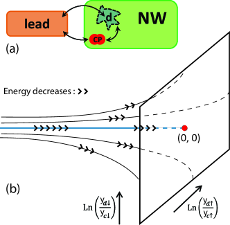
Figure 2: (color online) (a) Demonstration of tunneling into a Zero-energy impurity bound states (non-Majorana). $d$ and $CP$ represent ZEIBS and cooper pair, respectively. (b) Schematic representation of the flow diagram based on Eq.  (11). The arrows indicate the direction of the flow as energy decreases. The red dot in the center is the symmetric fixed point ($y_{d\uparrow}=y_{c\uparrow}$ and $y_{d\downarrow}=y_{c\downarrow}$), which is unstable. The edges of the parallelogram correspond to four stable fixed points. 1) ($y_{d\uparrow}$ perfect transmission, $y_{c\uparrow}=y_{d\downarrow}=y_{c\downarrow}=0$) at right edge. Note that $y_{d\downarrow}$ and $y_{c\downarrow}$ have the same power law decay rate, and therefore $\ln(y_{d\downarrow}/y_{c\downarrow})=\rm{constant}$ near the Fixed point. Other three fixed points are: 2) ($y_{c\uparrow}$ perfect transmission, $y_{d\uparrow}=y_{d\downarrow}=y_{c\downarrow}=0$); 3) ($y_{d\downarrow}$ perfect transmission, $y_{c\uparrow}=y_{d\uparrow}=y_{c\downarrow}=0$); 4) ($y_{c\downarrow}$ perfect transmission, $y_{c\uparrow}=y_{d\uparrow}=y_{d\downarrow}=0$).

Since the tunneling has only a single channel, the lead can be reduced to a semi-infinite free fermion field, which then can be unfolded to form a chiral free fermionic field Affleck (1995); we take the coupling to the SCNW to be $x=0$. Then, this field can be bosonized in a standard way Senechal (2003); Giamarchi (2004): $\Psi_{\rm L\sigma}(x)=F_{\sigma}\,e^{i\Phi_{\sigma}(x)}/\sqrt{2\pi}$, where $\Phi_{\sigma}(x)$ is a chiral bosonic field with $[\Phi_{\sigma}(x),\Phi_{\sigma^{\prime}}(x^{\prime})]=i\delta_{\sigma\sigma^{\prime}}\pi\,\rm{sgn}(x-x^{\prime})$, $F_{\sigma}$ is Klein factor. For a spinful lead, the Hamiltonian becomes

$$H = \sum_{\sigma}\frac{v_{F}}{4\pi}\int_{-\infty}^{\infty}dx\big{(}\partial_{x}\Phi_{\sigma}(x)\big{)}^{2}$$ (9)

$$+\Big{[}y_{\rm d,\sigma}\frac{F_{\sigma}e^{-i\Phi_{\sigma}(0)}}{\sqrt{2\pi}}d\,e^{-i\phi}+y_{\rm c,\sigma}\frac{F_{\sigma}e^{-i\Phi_{\sigma}(0)}}{\sqrt{2\pi}}d^{\dagger}e^{-i\phi}$$

$$+h.c.\Big{]}+K_{\sigma}(d^{\dagger}d-1/2)\partial_{x}\Phi_{\sigma}(x=0)/\pi.$$

The last term represents the density interaction between the lead (i.e. $\Psi_{\rm L\sigma}^{\dagger}(x)\Psi_{\rm L\sigma}(x)=-\partial_{x}\Phi_{\sigma}(x)/\pi$) and the localized ZEIBS, and this interaction is initially very small and can be enhanced in the RG processes. Since the correlation function of the phase $\phi$ shows the similar power law decay to the chiral bosonic field : $\langle e^{-i\phi(t)}e^{i\phi(0)}\rangle\sim t^{-2r}$ and $\langle e^{-i\Phi_{\sigma}(x=0,t)}e^{i\Phi_{\sigma}(x=0,0)}\rangle\sim t^{-1}$, we can combine the two bosonic field and introduce a new field Florens et al. (2007); Le Hur and Li (2005); Mebrahtu et al. (2012): $\widetilde{\Phi}_{\sigma}(x)=\sqrt{g}(\Phi_{\sigma}(x)+\phi(x))$ with $\quad g=1/(1+2r)$, which satisfies $\langle e^{-i\widetilde{\Phi}_{\sigma}(x=0,t)}e^{i\widetilde{\Phi}_{\sigma}(x=0,0)}\rangle\sim t^{-1}$. Note that only $\phi(x=0)=\phi$ has the physical meaning (i.e. phase fluctuation), and $\phi(x\neq 0)$ are auxiliary fields. Overall, we have $[\phi(x),\phi(x^{\prime})]=2ir\pi\,\rm{sgn}(x-x^{\prime})$. Since the tunneling involves only the phase $\phi(x=0)$, the conductance will not be affected by the auxiliary fields. Then, the Hamiltonian becomes

$$H =\sum_{\sigma}\frac{v_{F}}{4\pi}\int_{-\infty}^{\infty}dx\big{(}\partial_{x}\widetilde{\Phi}_{\sigma}(x)\big{)}^{2}$$ (10)

$$+\Big{[}y_{\rm d,\sigma}\frac{F_{\sigma}}{\sqrt{2\pi}}e^{-i\widetilde{\Phi}_{\sigma}(0)/\sqrt{g}}\,d+y_{\rm c,\sigma}\frac{F_{\sigma}}{\sqrt{2\pi}}e^{-i\widetilde{\Phi}_{\sigma}(0)/\sqrt{g}}d^{\dagger}$$

$$+h.c.\Big{]}+\frac{K_{\sigma}}{\sqrt{g}\pi}(d^{\dagger}d-1/2)\partial_{x}\widetilde{\Phi}_{\sigma}(0).$$

One can define a set of dimensionless parameters: $\widetilde{y}_{d,\sigma}=y_{d,\sigma}l/\sqrt{2\pi}$, $\widetilde{y}_{c,\sigma}=y_{c,\sigma}l/\sqrt{2\pi}$, and $\widetilde{K}_{\sigma}=2K_{\sigma}/(\pi v_{F})$, where $l$ is a short time cutoff in the scaling process. Following the dimension analysis and operator product expansion Cardy (1996); Senechal (2003); sup , one can simply obtain the RG equations in the weak tunneling limit

$$\frac{dy_{d,\sigma}}{d\ln l} = \Big{(}1-\frac{(1-\widetilde{K}_{\sigma})^{2}}{2g}-\frac{(\widetilde{K}_{-\sigma})^{2}}{2g}\Big{)}y_{d,\sigma},$$

$$\frac{dy_{c,\sigma}}{d\ln l} = \Big{(}1-\frac{(1+\widetilde{K}_{\sigma})^{2}}{2g}-\frac{(\widetilde{K}_{-\sigma})^{2}}{2g}\Big{)}y_{c,\sigma},$$

$$\frac{d\widetilde{K}_{\sigma}}{d\ln l} = 2(1-\widetilde{K}_{\sigma})\widetilde{y}_{d,\sigma}^{2}-2(1+\widetilde{K}_{\sigma})\widetilde{y}_{c,\sigma}^{2}$$ (11)

$$-2\widetilde{K}_{\sigma}\widetilde{y}_{d,-\sigma}^{2}-2\widetilde{K}_{\sigma}\widetilde{y}_{c,-\sigma}^{2}.$$

Five fixed points are obtained and shown in Fig. 2 (b). The first one corresponds to $\widetilde{K}_{\uparrow}=0$, $\widetilde{K}_{\downarrow}=-1$, $y_{d,\uparrow}=y_{d,\downarrow}=y_{c,\uparrow}=0$. In this case, $y_{c,\downarrow}$ will flow to perfect transmission, $dy_{d,\uparrow}/d\ln l=-2ry_{d,\uparrow}$, $dy_{d,\downarrow}/d\ln l=(-1-4r)y_{d,\downarrow}$, and $dy_{c,\uparrow}/d\ln l=-2ry_{c,\uparrow}$. The leading tunneling process corresponds to $y_{d,\uparrow}\cdot y_{c,\downarrow}$, i.e. a spin-up electron entering the ZEIBS from the lead, then hopping out to form a cooper pair with another spin-down electron from the lead. Therefore, the zero-voltage conductance shows a power law decay $G\sim T^{2r}$ near $T=0$. The finite voltage bias will cut off the scaling, and thus the ZBP will split at low $T$. Conductance shows the same power law decay for three other similar fixed points. Unless the initial condition $y_{d,\sigma}=y_{c,\sigma}$ is satisfied, the system will flow to one of these four fixed points.

If the bare parameters reach a symmetric point: $K_{\sigma}=0$ and $y_{d,\sigma}=y_{c,\sigma}$, all the tunneling strength $y_{d(c),\sigma}$ is relevant and will flow to perfect transmission (i.e. perfect Andreev reflection); this condition leads to an unstable critical point which belongs to the same universal class as the case of tunneling into a MF. By noting the similarity between our model (i.e. Eq. 10) and the case with a Luttinger liquid lead sup , one can obtain the $V=0$ conductance for this symmetric point (or for MF) in the strong coupling limit (low $T$) sup ; Fidkowski et al. (2012): $2e^{2}/h-G\sim T^{(2-4r)/(1+2r)}$. For ZEIBS, the condition $y_{d,\sigma}=y_{c,\sigma}$ requires fine tuning both the tunneling barrier and spin components, and thus its realization is extremely difficult.

Tunneling into a cluster of mid-gap states — If both the spin rotation and time reversal symmetries are broken in SCNW, disorder can induce a cluster of mid-gap states around zero energy localized near the end of the wire Bagrets and Altland (2012); Liu et al. (2012); Neven et al. (2013). Therefore, even without a zero energy state (either MF or ZEIBS), the tunneling conductance shows a zero-energy peak at finite $T$ without dissipation effect. To study the dissipation effects for those cases, we consider the tunneling Hamiltonian in Eq. (3), and treat the tunneling strength $y$ as a small parameter such that the perturbation theory can be applied. This assumption is valid for tunneling into any non-MF state (with a small bare tunneling strength) except at the highly symmetric situation shown in the previous section.

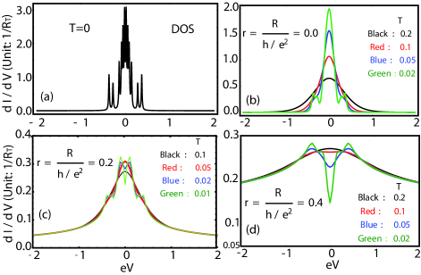
Figure 3: (color online) Differential conductance $dI/dV$ (tunneling into a cluster of mid-gap states around zero energy) as a function of applied voltage $V$. (a) An arbitrary choice of the DOS for a cluster of states, which is also the $T=0$ conductance for $r=0$. (b) The $r=0$ finite temperature conductance. The conductance with dissipation effect, i.e. $r=0.2$ (c) and $r=0.4$ (d), for different temperatures. The single peak splits into two as $T$ decreases.

The current operator for the junction is $\hat{I}=i[H_{T},\sum_{k\sigma}c^{\dagger}_{k\sigma}c_{k\sigma}]=-i\sum_{k\sigma,\nu}(y_{k\sigma,\nu}c^{\dagger}_{k\sigma}b_{\nu}e^{-i\phi}-h.c.)$ Then, the current through the junction up to the leading order in tunneling strength is given by Kubo formula (this can also be obtained by golden rule Ingold and Yu.V. (1992))

$$I(t) = -i\int_{-\infty}^{\infty}dt^{\prime}\,\theta(t-t^{\prime})\;\langle[\hat{I}(t),H_{T}(t^{\prime})]\rangle_{0}$$ (12)

$$= \int_{-\infty}^{\infty}\frac{d\omega_{1}}{2\pi}\int_{-\infty}^{\infty}\frac{d\omega_{2}}{2\pi}\sum_{k\sigma,\nu}|y_{k\sigma,\nu}|^{2}A_{k\sigma}^{L}(\omega_{1})A_{\nu}^{SCNW}(\omega_{2})$$

$$\times\{[1-f(\omega_{1}-eV)]f(\omega_{2})P(\omega_{2}-\omega_{1})$$

$$-f(\omega_{1}-eV)[1-f(\omega_{2})]P(\omega_{1}-\omega_{2})\}.$$

with

$$P(\omega)=\frac{1}{2\pi}\int_{-\infty}^{\infty}dt\exp[i\omega t+J(t)]$$ (13)

where $J(t)=\langle\phi(t)\phi(0)\rangle-\langle\phi^{2}\rangle$ (see Ingold and Yu.V. (1992); sup for more details) and $\langle\cdots\rangle_{0}$ indicates the average without the tunneling term. $P(\omega)$ describes the energy emission and absorption in the electron tunneling processes due to dissipation effects. $A_{k\sigma}^{L}(\omega_{1})$ is the spectral function of the lead, and we assume a constant density of state (DOS): $\sum_{k\sigma}|y_{k\sigma,\nu}|^{2}A_{k\sigma}^{L}(\omega_{1})=1/(eR_{T})$, where $R_{T}$ can be viewed as the tunneling resistance. $f$ is the Fermi-distribution function. Without dissipation, i.e. $r=0$, at zero temperature one obtain $dI/dV\propto\sum_{\nu}A_{\nu}^{SCNW}(\omega_{2})$ which gives the DOS of the wire. A realization of the DOS (i.e. $T=0$ conductance for $r=0$), is shown in Fig. 3 (a). For finite temperature, this cluster of states results in a ZBP as shown in Fig. 3 (b). As temperature decreases (still larger than the level spacing of the mid-gap states), the ZBP height increases for $r=0$, which is similar to Majorana ZBP. This feature changes dramatically when the dissipation effect is included. As shown in Fig. 3 (c) $r=0.2$ and (d) $r=0.4$ ($R\sim k\Omega$), the single conductance peak splits into two peaks and zero bias conductance decreases as temperature goes down; and this feature is contrary to that of Majorana ZBP : The zero bias conductance for $r<1/2$ increases as $T$ goes down and finally approaches $2e^{2}/h$ at $T=0$. Fig. 3 (c) and (d) also show that the peak splitting occurs at higher $T$ for larger $r$.

Discussion — Tunneling into a MF is equivalent to the resonant tunneling between an electron lead and a hole lead Law et al. (2009) (also see Eq. (6)) with exactly the symmetric tunneling barriers due to the topological properities of MF. With ohmic dissipation, the resonant tunneling shows non-trivial phase diagrams Mebrahtu et al. (2012); Liu et al. (2013b): 1) any asymmetry in the barriers induces a relevant backscattering which destroys the resonant tunneling; 2) this backscattering vanishes for a special symmetric point, and the next leading term is irrelevant for small $r$ ($r<1/2$ for our case). This symmetry, which results in dissipative resonant tunneling, is topologically protected by MF; it is not protected for other cases, and requires fine tuning. In the experiments Mourik et al. (2012); Deng et al. (2012); Das et al. (2012), the metal lead can be made rather resistive ($R\sim k\Omega$, but need $r<1/2$), by using e.g. $\rm{Cr/Au}$ film Mebrahtu et al. (2012, 2013). When coupling to a MF zero mode, the height of ZBP increases as $T$ goes down: $2e^{2}/h-G\sim T^{(2-4r)/(1+2r)}$ near $T=0$, and $G\sim T^{2r-1}$ for high $T$. When coupling to a non-MF mode causing a ZBP, however, its height shows a power law suppression at low $T$: $G\sim T^{2r}$.

D.E.L. is grateful to H.U.Baranger and A. Levchenko for valuable discussions and suggestions. The author acknowledges support from US DOE, Division of Materials Sciences and Engineering, under Grant No. DE-SC0005237, Michigan state university, and ARO through contract W911NF-12-1-023.

References

- Fu and Kane (2008) L. Fu and C. L. Kane, Phys. Rev. Lett. 100, 096407 (2008).
- Sau et al. (2010) J. D. Sau, R. M. Lutchyn, S. Tewari, and S. Das Sarma, Phys. Rev. Lett. 104, 040502 (2010).
- Alicea (2010) J. Alicea, Phys. Rev. B 81, 125318 (2010).
- Lutchyn et al. (2010) R. M. Lutchyn, J. D. Sau, and S. Das Sarma, Phys. Rev. Lett. 105, 077001 (2010).
- Oreg et al. (2010) Y. Oreg, G. Refael, and F. von Oppen, Phys. Rev. Lett. 105, 177002 (2010).
- Sato et al. (2009) M. Sato, Y. Takahashi, and S. Fujimoto, Phys. Rev. Lett. 103, 020401 (2009).
- Zhu et al. (2011) S.-L. Zhu, L.-B. Shao, Z. D. Wang, and L.-M. Duan, Phys. Rev. Lett. 106, 100404 (2011).
- Jiang et al. (2011a) L. Jiang, T. Kitagawa, J. Alicea, A. R. Akhmerov, D. Pekker, G. Refael, J. I. Cirac, E. Demler, M. D. Lukin, and P. Zoller, Phys. Rev. Lett. 106, 220402 (2011a).
- Reynoso and Frustaglia (2013) A. A. Reynoso and D. Frustaglia, Phys. Rev. B 87, 115420 (2013).
- Liu et al. (2013a) D. E. Liu, A. Levchenko, and H. U. Baranger, Phys. Rev. Lett. 111, 047002 (2013a).
- Das Sarma et al. (2006) S. Das Sarma, C. Nayak, and S. Tewari, Phys. Rev. B 73, 220502 (2006).
- Fu and Kane (2009a) L. Fu and C. L. Kane, Phys. Rev. Lett. 102, 216403 (2009a).
- Fu and Kane (2009b) L. Fu and C. L. Kane, Phys. Rev. B 79, 161408 (2009b).
- Akhmerov et al. (2009) A. R. Akhmerov, J. Nilsson, and C. W. J. Beenakker, Phys. Rev. Lett. 102, 216404 (2009).
- Law et al. (2009) K. T. Law, P. A. Lee, and T. K. Ng, Phys. Rev. Lett. 103, 237001 (2009).
- Akhmerov et al. (2011) A. R. Akhmerov, J. P. Dahlhaus, F. Hassler, M. Wimmer, and C. W. J. Beenakker, Phys. Rev. Lett. 106, 057001 (2011).
- M. et al. (2011) W. M., A. Akhmerov, J. P. Dahlhaus, and C. W. J. Beenakker, New Journal of Physics 13, 053016 (2011).
- Liu and Baranger (2011) D. E. Liu and H. U. Baranger, Phys. Rev. B 84, 201308 (2011).
- Jiang et al. (2011b) L. Jiang, D. Pekker, J. Alicea, G. Refael, Y. Oreg, and F. von Oppen, Phys. Rev. Lett. 107, 236401 (2011b).
- Fidkowski et al. (2012) L. Fidkowski, J. Alicea, N. H. Lindner, R. M. Lutchyn, and M. P. A. Fisher, Phys. Rev. B 85, 245121 (2012).
- San-Jose et al. (2012) P. San-Jose, E. Prada, and R. Aguado, Phys. Rev. Lett. 108, 257001 (2012).
- Mourik et al. (2012) V. Mourik, K. Zuo, S. M. Frolov, S. R. Plissard, E. P. A. M. Bakkers, and L. P. Kouwenhoven, Science 336, 1003 (2012).
- Deng et al. (2012) M. T. Deng, C. L. Yu, G. Y. Huang, M. Larsson, P. Caroff, and H. Q. Xu, Nano Letters 12, 6414 (2012).
- Das et al. (2012) A. Das, Y. Ronen, Y. Most, Y. Oreg, M. Heiblum, and H. Shtrikman, Nat. Phys. 8, 887 (2012).
- Bagrets and Altland (2012) D. Bagrets and A. Altland, Phys. Rev. Lett. 109, 227005 (2012).
- Liu et al. (2012) J. Liu, A. C. Potter, K. T. Law, and P. A. Lee, Phys. Rev. Lett. 109, 267002 (2012).
- Neven et al. (2013) P. Neven, D. Bagrets, and A. Altland, New Journal of Physics 15, 055019 (2013).
- Feynman and Vernon (1963) R. Feynman and F. Vernon, Annals of physics 24, 118 (1963).
- Leggett et al. (1987) A. J. Leggett, S. Chakravarty, A. T. Dorsey, M. P. A. Fisher, A. Garg, and W. Zwerger, Rev. Mod. Phys. 59, 1 (1987).
- Ingold and Yu.V. (1992) G.-L. Ingold and N. Yu.V., in Single Charge Tunneling: Coulomb Blockade Phenomena in Nanostructures, edited by H. Grabert and M. H. Devoret (Plenum Press, New York, 1992), vol. 294, pp. 21–107.
- Mebrahtu et al. (2012) H. T. Mebrahtu, I. V. Borzenets, D. E. Liu, H. Zheng, Y. V. Bomze, A. I. Smirnov, H. Baranger, and G. Finkelstein, Nature 488, 61 (2012).
- Mebrahtu et al. (2013) H. T. Mebrahtu, I. V. Borzenets, H. Zheng, Y. V. Bomze, A. I. Smirnov, S. Florens, H. U. Baranger, and G. Finkelstein, Nat. Phys. advance online publication (2013), arXiv:1212.3857.
- Liu et al. (2013b) D. E. Liu, H. Zheng, G. Finkelstein, and H. U. Baranger, arXiv:1310.4773 (2013b).
- Caldeira and Leggett (1981) A. O. Caldeira and A. J. Leggett, Phys. Rev. Lett. 46, 211 (1981).
- Hewson (1997) A. Hewson, The Kondo problem to heavy fermions (Cambridge Univ. Press, 1997).
- Affleck (1995) I. Affleck, Acta Phys. Polon. B 26, 1869 (1995), arXiv:cond-mat/9512099.
- Senechal (2003) D. Senechal, in Theoretical Methods for Strongly Correlated Electrons (2003), arXiv:cond-mat/9908262.
- Giamarchi (2004) T. Giamarchi, Quantum Physics in One Dimension (Oxford Univ. Press, 2004).
- Florens et al. (2007) S. Florens, P. Simon, S. Andergassen, and D. Feinberg, Phys. Rev. B 75, 155321 (2007).
- Le Hur and Li (2005) K. Le Hur and M.-R. Li, Phys. Rev. B 72, 073305 (2005).
- Cardy (1996) J. Cardy, Scaling and Renormalization in Statistical Physics (Cambridge Univ. Press, 1996), page 83-90.
- (42) See supplementary materials for further details.