High-order algorithms for solving eigenproblems over discrete surfaces

Sheng-Gwo Chen Mei-Hsiu Chi mhchi@math.ccu.edu.tw Jyh-Yang Wu jywu@math.ccu.edu.tw Department of Applied Mathematics, National Chiayi University, Chia-Yi 600, Taiwan. Department of Mathematics, National Chung Cheng University, Chia-Yi 621, Taiwan.
Abstract

The eigenvalue problem of the Laplace-Beltrami operators on curved surfaces plays an essential role in the convergence analysis of the numerical simulations of some important geometric partial differential equations which involve this operator. In this note we shall combine the local tangential lifting (LTL) method with the configuration equation to develop a new effective and convergent algorithm to solve the eigenvalue problems of the Laplace-Beltrami operators acting on functions over discrete surfaces. The convergence rates of our algorithms of discrete Laplace-Beltrami operators over surfaces is O(rn)𝑂superscript𝑟𝑛O(r^{n}), n1𝑛1n\geq 1, where r𝑟r represents the size of the mesh of discretization of the surface. The problem of high-order accuracies will also be discussed and used to compute geometric invariants of the underlying surfaces. Some convergence tests and eigenvalue computations on the sphere, tori and a dumbbell are presented.

keywords:
Eigenproblem, Local tangential lifting method, Configuration equation, Discrete Laplace-Beltrami operator.
journal:

1 Introduction

Let ΣΣ\Sigma be a smooth regular surface in the 3D space. The Laplace-Beltrami (LB) operator is a natural generalization of the classical Laplacian ΔΣsubscriptΔΣ\Delta_{\Sigma} from the Euclidean space to a curved space. To understand the LB operators on curved surfaces, it is natural to investigate their associated eigenvalue problems:

ΔΣϕ=λϕ.subscriptΔΣitalic-ϕ𝜆italic-ϕ\Delta_{\Sigma}\phi=\lambda\phi. (1)

Or, more generally,

Σ(hΣϕ)=λϕsubscriptΣsubscriptΣitalic-ϕ𝜆italic-ϕ\nabla_{\Sigma}\cdot(h\nabla_{\Sigma}\phi)=\lambda\phi (2)

where hh is C2superscript𝐶2C^{2} real function on ΣΣ\Sigma.

The eigenvalue problem of the LB operator plays important roles not just in the study of geometric properties of curved spaces, but also in many applications in the fields of physics, engineering and computer science. The LB operator has recently many applications in a variety of different areas, such as surface processing[6, 14], signal processing[12] and geometric partial differential equations[7].

Since the objective underlying surfaces to be considered are usually represented as discrete meshes in these applications, it is useful in practice to discretize the LB operators and solving the eigenproblems over discrete surfaces. There are many approaches for estimating Laplace-Beltrami operator and solving the Laplace-Beltrami eigenproblems [16, 17]. In 2011, Macdonald[10] proposed an elegant method to solve the Laplace-Bletrami eigenproblems for Equations (1) and (2) by the closest point method[13]. In this paper we shall describe simple and effective methods with high-order accuracies to define the discrete LB operator on functions on a triangular mesh.

In 2012, Ray et al.[15] used the method of least square to obtain high-order approximations of derivatives and integrations. In this paper, we shall use ideas developed in Chen, Chi and Wu[3, 4] where we try to estimate the discrete partial derivatives of functions on 2D scattered data points. Indeed, the ideas that we shall use to develop our algorithms are divided into two main steps: first we lift the 1-neighborhood points to the approximating tangent space and obtain a local tangential polygon. Second, we use some geometric idea to lift functions to the tangent space. We call this a local tangential lifting (LTL) method[5, 19]. Then we present a new algorithm, the configuration method, to compute their Laplacians in the 2D tangent space. This means that the LTL process allows us to reduce the 2D curved surface problem to the 2D Euclidean problem.

In other words, we shall combine the local tangential lifting (LTL) method with the configuration equation to develop a new effective and convergent algorithm to solve the eigenpair problems of the Laplace-Beltrami operators acting on functions over curved surfaces. We shall also present a mathematical proof of the convergence of our algorithm. Our algorithm is not only conceptually simple, but also easy to implement. Indeed, the convergence rate of our new algorithms of discrete Laplace-Beltrami operators over surfaces is O(rn)𝑂superscript𝑟𝑛O(r^{n}), n1𝑛1n\geq 1, where r𝑟r represents the size of the mesh of discretization of the surface. In section 2, we introduce the gradient of a function, the divergence of a vector field and the Laplace-Beltrami operator on regular surfaces. Our O(r)𝑂𝑟O(r)-LTL configuration method is discussed in section 3. In section 4, we discuss how to improve the methods to have high-order accuracies. We also give some numerical simulations to support these results in section 5.

2 The gradient, divergence, and Laplace-Beltrami operator

In order to describe the gradient, divergence and the LB operator on functions or vector fields in a regular surface ΣΣ\Sigma in the 3D Euclidean space 3superscript3\mathbb{R}^{3}, we consider a parameterization 𝐱:UΣ:𝐱𝑈Σ\mathbf{x}:U\rightarrow\Sigma at a point 𝐩𝐩\mathbf{p}, where U𝑈U is an open subset of the 2D Euclidean space 2superscript2\mathbb{R}^{2}. We can choose, at each point 𝐪𝐪\mathbf{q} of 𝐱(U)𝐱𝑈\mathbf{x}(U), a unit normal vector 𝐍(𝐪)𝐍𝐪\mathbf{N}(\mathbf{q}). The map 𝐍:𝐱(U)𝕊2:𝐍𝐱𝑈superscript𝕊2\mathbf{N}:\mathbf{x}(U)\rightarrow\mathbb{S}^{2} is the local Gauss map from an open subset of the regular surface ΣΣ\Sigma to the unit sphere 𝕊2superscript𝕊2\mathbb{S}^{2} in the 3D Euclidean space 3superscript3\mathbb{R}^{3}. Denote the tangent space of ΣΣ\Sigma at the point 𝐩𝐩\mathbf{p} by TΣ𝐩={𝐯3|𝐯𝐍(𝐩)}𝑇subscriptΣ𝐩conditional-set𝐯superscript3bottom𝐯𝐍𝐩T\Sigma_{\mathbf{p}}=\{\mathbf{v}\in\mathbb{R}^{3}|\mathbf{v}\bot\mathbf{N}(\mathbf{p})\}. The tangent space TΣ𝐩𝑇subscriptΣ𝐩T\Sigma_{\mathbf{p}} is a linear space spanned by {𝐱u,𝐱v}subscript𝐱𝑢subscript𝐱𝑣\{\mathbf{x}_{u},\mathbf{x}_{v}\} where u,v𝑢𝑣u,v are coordinates for U𝑈U.

The gradient ΣgsubscriptΣ𝑔\nabla_{\Sigma}g of a smooth function g𝑔g on ΣΣ\Sigma can be computed from

Σg=guGgvFEGF2𝐱u+gvEguFEGF2𝐱vsubscriptΣ𝑔subscript𝑔𝑢𝐺subscript𝑔𝑣𝐹𝐸𝐺superscript𝐹2subscript𝐱𝑢subscript𝑔𝑣𝐸subscript𝑔𝑢𝐹𝐸𝐺superscript𝐹2subscript𝐱𝑣\nabla_{\Sigma}g=\frac{g_{u}G-g_{v}F}{EG-F^{2}}\mathbf{x}_{u}+\frac{g_{v}E-g_{u}F}{EG-F^{2}}\mathbf{x}_{v} (3)

where E,F𝐸𝐹E,F, and G𝐺G are the coefficients of the first fundamental form and

gu=g(𝐱(u,v))u and gv=g(𝐱(u,v))v.subscript𝑔𝑢𝑔𝐱𝑢𝑣𝑢 and subscript𝑔𝑣𝑔𝐱𝑢𝑣𝑣g_{u}=\frac{\partial g(\mathbf{x}(u,v))}{\partial u}\mbox{ and }g_{v}=\frac{\partial g(\mathbf{x}(u,v))}{\partial v}. (4)

See do Carmo[8, 9] for the details.

Let 𝐗=A𝐱u+B𝐱v𝐗𝐴subscript𝐱𝑢𝐵subscript𝐱𝑣\mathbf{X}=A\mathbf{x}_{u}+B\mathbf{x}_{v} be a local vector field on ΣΣ\Sigma. The divergence, Σ𝐗subscriptΣ𝐗\nabla_{\Sigma}\cdot\mathbf{X}, of 𝐗𝐗\mathbf{X} is defined as a function Σ𝐗:Σ:subscriptΣ𝐗Σ\nabla_{\Sigma}\cdot\mathbf{X}:\Sigma\rightarrow\mathbb{R} given by the trace of the linear mapping 𝐘(𝐩)𝐘(𝐩)𝐗𝐘𝐩subscript𝐘𝐩𝐗\mathbf{Y}(\mathbf{p})\rightarrow\nabla_{\mathbf{Y}(\mathbf{p})}\mathbf{X} for 𝐩Σ𝐩Σ\mathbf{p}\in\Sigma. A direct computation gives

ΣX=1EGF2(u(AEGF2)+v(BEGF2)).subscriptΣ𝑋1𝐸𝐺superscript𝐹2𝑢𝐴𝐸𝐺superscript𝐹2𝑣𝐵𝐸𝐺superscript𝐹2\nabla_{\Sigma}\cdot X=\frac{1}{\sqrt{EG-F^{2}}}\left(\frac{\partial}{\partial u}(A\sqrt{EG-F^{2}})+\frac{\partial}{\partial v}(B\sqrt{EG-F^{2}})\right). (5)

The LB operator acting on the function g𝑔g is defined by

ΔΣg=ΣΣg.subscriptΔΣ𝑔subscriptΣsubscriptΣ𝑔\Delta_{\Sigma}g=\nabla_{\Sigma}\cdot\nabla_{\Sigma}g. (6)

for all smooth function g𝑔g on ΣΣ\Sigma. A direct computation yields the following local representation for the LB operator on a smooth function g𝑔g:

ΔΣg=1EGF2[u(GEGF2gu)u(FEGF2gv)]+1EGF2[v(EEGF2gv)v(FEGF2gu)].subscriptΔΣ𝑔absent1𝐸𝐺superscript𝐹2delimited-[]𝑢𝐺𝐸𝐺superscript𝐹2𝑔𝑢𝑢𝐹𝐸𝐺superscript𝐹2𝑔𝑣missing-subexpressionmissing-subexpressionmissing-subexpression1𝐸𝐺superscript𝐹2delimited-[]𝑣𝐸𝐸𝐺superscript𝐹2𝑔𝑣𝑣𝐹𝐸𝐺superscript𝐹2𝑔𝑢\begin{array}[]{ll}\Delta_{\Sigma}g=&\frac{1}{\sqrt{EG-F^{2}}}\left[\frac{\partial}{\partial u}(\frac{G}{\sqrt{EG-F^{2}}}\frac{\partial g}{\partial u})-\frac{\partial}{\partial u}(\frac{F}{\sqrt{EG-F^{2}}}\frac{\partial g}{\partial v})\right]\cr\cr&+\frac{1}{\sqrt{EG-F^{2}}}\left[\frac{\partial}{\partial v}(\frac{E}{\sqrt{EG-F^{2}}}\frac{\partial g}{\partial v})-\frac{\partial}{\partial v}(\frac{F}{\sqrt{EG-F^{2}}}\frac{\partial g}{\partial u})\right].\end{array} (7)

3 An O(r)𝑂𝑟O(r)-LTL configuration method

In this section, we shall introduce a new algorithm to solve the eigenpair problems, Equations (1) and (2), by the LTL configuration method.

Consider a triangular surface mesh S=(V,F)𝑆𝑉𝐹S=(V,F), where V={𝐯i|1inV}𝑉conditional-setsubscript𝐯𝑖1𝑖subscript𝑛𝑉V=\{\mathbf{v}_{i}|1\leq i\leq n_{V}\} is the list of vertices and F={Tk|1knF}𝐹conditional-setsubscript𝑇𝑘1𝑘subscript𝑛𝐹F=\{T_{k}|1\leq k\leq n_{F}\} is the list of triangles.

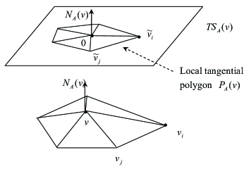
To describe the local tangential lifting (LTL) method, we introduce the approximating tangent plane TSA(𝐯)𝑇subscript𝑆𝐴𝐯TS_{A}(\mathbf{v}) and the local tangential polygon PA(𝐯)subscript𝑃𝐴𝐯P_{A}(\mathbf{v}) at the vertex 𝐯𝐯\mathbf{v} of S𝑆S as follows:

  1. 1.

    The normal vector 𝐍A(𝐯)subscript𝐍𝐴𝐯\mathbf{N}_{A}(\mathbf{v}) at the vertex 𝐯𝐯\mathbf{v} in S𝑆S is given by

    𝐍A(𝐯)=TT(𝐯)ωT𝐍TTT(𝐯)ωT𝐍Tsubscript𝐍𝐴𝐯subscript𝑇𝑇𝐯subscript𝜔𝑇subscript𝐍𝑇normsubscript𝑇𝑇𝐯subscript𝜔𝑇subscript𝐍𝑇\mathbf{N}_{A}(\mathbf{v})=\frac{\sum_{T\in T(\mathbf{v})}\omega_{T}\mathbf{N}_{T}}{\|\sum_{T\in T(\mathbf{v})}\omega_{T}\mathbf{N}_{T}\|} (8)

    where T(𝐯)𝑇𝐯T(\mathbf{v}) is the set of triangles that contain the vertex 𝐯𝐯\mathbf{v}, 𝐍Tsubscript𝐍𝑇\mathbf{N}_{T} is the unit normal to a triangle face T𝑇T with 𝐍T,𝐍T>0subscript𝐍𝑇superscriptsubscript𝐍𝑇0\langle\mathbf{N}_{T},\mathbf{N}_{T}^{\prime}\rangle>0 for all T,TT(𝐯)𝑇superscript𝑇𝑇𝐯T,T^{\prime}\in T(\mathbf{v}) and the centroid weight is given in [1, 2] by

    ωT=1𝐆T𝐯2T~T(𝐯)1𝐆T~𝐯2subscript𝜔𝑇1superscriptnormsubscript𝐆𝑇𝐯2subscript~𝑇𝑇𝐯1superscriptnormsubscript𝐆~𝑇𝐯2\omega_{T}=\frac{\frac{1}{\|\mathbf{G}_{T}-\mathbf{v}\|^{2}}}{\sum_{\tilde{T}\in T(\mathbf{v})}\frac{1}{\|\mathbf{G}_{\tilde{T}}-\mathbf{v}\|^{2}}} (9)

    where 𝐆Tsubscript𝐆𝑇\mathbf{G}_{T} is the centroid of the triangle face T𝑇T determined by

    𝐆T=𝐯+𝐯i+𝐯j3.subscript𝐆𝑇𝐯subscript𝐯𝑖subscript𝐯𝑗3\mathbf{G}_{T}=\frac{\mathbf{v}+\mathbf{v}_{i}+\mathbf{v}_{j}}{3}. (10)

    Note that the letter A𝐴A in the notation 𝐍A(v)subscript𝐍𝐴𝑣\mathbf{N}_{A}(v) stands for the word ”Approximation”.

  2. 2.

    The approximating tangent plane TSA(𝐯)𝑇subscript𝑆𝐴𝐯TS_{A}(\mathbf{v}) of S𝑆S at 𝐯𝐯\mathbf{v} is now determined by TSA(𝐯)={𝐰3|𝐰𝐍A(𝐯)}𝑇subscript𝑆𝐴𝐯conditional-set𝐰superscript3bottom𝐰subscript𝐍𝐴𝐯TS_{A}(\mathbf{v})=\{\mathbf{w}\in\mathbb{R}^{3}|\mathbf{w}\bot\mathbf{N}_{A}(\mathbf{v})\}.

  3. 3.

    The local tangential polygon PA(𝐯)subscript𝑃𝐴𝐯P_{A}(\mathbf{v}) of 𝐯𝐯\mathbf{v} in TSA(𝐯)𝑇subscript𝑆𝐴𝐯TS_{A}(\mathbf{v}) is formed by the vertices 𝐯¯isubscript¯𝐯𝑖\bar{\mathbf{v}}_{i} which is the lifting vertex of 𝐯isubscript𝐯𝑖\mathbf{v}_{i} adjacent to 𝐯𝐯\mathbf{v} in V𝑉V:

    𝐯¯i=(𝐯i𝐯)<𝐯i𝐯,𝐍A(𝐯)>𝐍A(𝐯)formulae-sequencesubscript¯𝐯𝑖limit-fromsubscript𝐯𝑖𝐯subscript𝐯𝑖𝐯subscript𝐍𝐴𝐯subscript𝐍𝐴𝐯\bar{\mathbf{v}}_{i}=(\mathbf{v}_{i}-\mathbf{v})-<\mathbf{v}_{i}-\mathbf{v},\mathbf{N}_{A}(\mathbf{v})>\mathbf{N}_{A}(\mathbf{v}) (11)

    as in figure 1.

    Refer to caption
    Figure 1: The local tangential polygon PA(𝐯)subscript𝑃𝐴𝐯P_{A}(\mathbf{v})
  4. 4.

    We can choose an orthonormal basis 𝐞1,𝐞2subscript𝐞1subscript𝐞2\mathbf{e}_{1},\mathbf{e}_{2} for the tangent plane TSA(𝐯)𝑇subscript𝑆𝐴𝐯TS_{A}(\mathbf{v}) of S𝑆S at 𝐯𝐯\mathbf{v} and obtain an orthonormal coordinates (x,y)𝑥𝑦(x,y) for vectors 𝐰TSA(𝐯)𝐰𝑇subscript𝑆𝐴𝐯\mathbf{w}\in TS_{A}(\mathbf{v}) by 𝐰=x𝐞1+y𝐞2𝐰𝑥subscript𝐞1𝑦subscript𝐞2\mathbf{w}=x\mathbf{e}_{1}+y\mathbf{e}_{2}. We set 𝐯¯i=xi𝐞1+yi𝐞2subscript¯𝐯𝑖subscript𝑥𝑖subscript𝐞1subscript𝑦𝑖subscript𝐞2\bar{\mathbf{v}}_{i}=x_{i}\mathbf{e}_{1}+y_{i}\mathbf{e}_{2} with respect to the orthonormal basis 𝐞1,𝐞2subscript𝐞1subscript𝐞2\mathbf{e}_{1},\mathbf{e}_{2}.

Now we explain how to lift locally a function defined on V𝑉V to the local tangential polygon PA(𝐯)subscript𝑃𝐴𝐯P_{A}(\mathbf{v}). Consider a function ϕitalic-ϕ\phi on V𝑉V. We will lift locally the function ϕitalic-ϕ\phi to a function of two variables , denoted by ϕ¯¯italic-ϕ\bar{\phi}, on the vertices 𝐯¯isubscript¯𝐯𝑖\bar{\mathbf{v}}_{i} in PA(𝐯)subscript𝑃𝐴𝐯P_{A}(\mathbf{v}) by simply setting

ϕ¯(xi,yi)=ϕ(𝐯i)¯italic-ϕsubscript𝑥𝑖subscript𝑦𝑖italic-ϕsubscript𝐯𝑖\bar{\phi}(x_{i},y_{i})=\phi(\mathbf{v}_{i}) (12)

and ϕ¯(0)=ϕ(𝐯)¯italic-ϕ0italic-ϕ𝐯\bar{\phi}(\vec{0})=\phi(\mathbf{v}) where 00\vec{0} is the origin of TSA(𝐯)𝑇subscript𝑆𝐴𝐯TS_{A}(\mathbf{v}) . Then one can extend the function ϕ¯¯italic-ϕ\bar{\phi} to be a piecewise linear function on the whole polygon PA(𝐯)subscript𝑃𝐴𝐯P_{A}(\mathbf{v}) in a natural and obvious way.

Next, we introduce the configuration matrices for ΔΣϕsubscriptΔΣitalic-ϕ\Delta_{\Sigma}\phi and Σ(hΣϕ)subscriptΣsubscriptΣitalic-ϕ\nabla_{\Sigma}\cdot(h\nabla_{\Sigma}\phi) in Equations (1) and (2).

3.1 The Configuration matrix for ΔΣϕsubscriptΔΣitalic-ϕ\Delta_{\Sigma}\phi

According to the LTL method, the differential quantities at a point on curved surfaces correspond to planar differential quantities in 2superscript2\mathbb{R}^{2}. Hence, we only need to estimate the Laplace-Beltrami operator on planar triangular meshes. Given a C3superscript𝐶3C^{3} function f𝑓f on an open domain Ω2Ωsuperscript2\Omega\subset\mathbb{R}^{2} with the origin (0,0)Ω00Ω(0,0)\in\Omega, Taylor’s expansion for two variables x𝑥x and y𝑦y gives

f(x,y)=f(0,0)+xfx(0,0)+yfy(0,0)+x22fxx(0,0)+xyfxy(0,0)+y22fyy(0,0)+O(r3)𝑓𝑥𝑦absent𝑓00𝑥subscript𝑓𝑥00𝑦subscript𝑓𝑦00missing-subexpressionmissing-subexpressionmissing-subexpressionsuperscript𝑥22subscript𝑓𝑥𝑥00𝑥𝑦subscript𝑓𝑥𝑦00missing-subexpressionmissing-subexpressionmissing-subexpressionsuperscript𝑦22subscript𝑓𝑦𝑦00𝑂superscript𝑟3\begin{array}[]{rl}f(x,y)=&f(0,0)+xf_{x}(0,0)+yf_{y}(0,0)\cr\cr&+\frac{x^{2}}{2}f_{xx}(0,0)+xyf_{xy}(0,0)\cr\cr&+\frac{y^{2}}{2}f_{yy}(0,0)+O(r^{3})\end{array} (13)

when r=x2+y2𝑟superscript𝑥2superscript𝑦2r=x^{2}+y^{2} is small.

Consider a family of neighboring points (xj,yj)Ωsubscript𝑥𝑗subscript𝑦𝑗Ω(x_{j},y_{j})\in\Omega, j=1,2,,n𝑗12𝑛j=1,2,\cdots,n, of the origin (0,0)00(0,0). Take some constants αjsubscript𝛼𝑗\alpha_{j}, j=1,2,,n𝑗12𝑛j=1,2,\cdots,n, with j=1nαj=ϵ0subscriptsuperscript𝑛𝑗1subscript𝛼𝑗italic-ϵ0\sum^{n}_{j=1}\alpha_{j}=\epsilon\neq 0. Then one has

j=1nαj(f(xj,yj)f(0,0))=(j=1nαjxj)fx(0,0)+(j=1nαjyj)fy(0,0)+12(j=1nαjxj2)fxx(0,0)+(j=1nαjxjyj)fxy(0,0)+12(j=1nαjyj2)fyy(0,0)+O(r3),missing-subexpressionsuperscriptsubscript𝑗1𝑛subscript𝛼𝑗𝑓subscript𝑥𝑗subscript𝑦𝑗𝑓00missing-subexpressionmissing-subexpressionsuperscriptsubscript𝑗1𝑛subscript𝛼𝑗subscript𝑥𝑗subscript𝑓𝑥00superscriptsubscript𝑗1𝑛subscript𝛼𝑗subscript𝑦𝑗subscript𝑓𝑦00missing-subexpressionmissing-subexpressionmissing-subexpression12superscriptsubscript𝑗1𝑛subscript𝛼𝑗superscriptsubscript𝑥𝑗2subscript𝑓𝑥𝑥00superscriptsubscript𝑗1𝑛subscript𝛼𝑗subscript𝑥𝑗subscript𝑦𝑗subscript𝑓𝑥𝑦00missing-subexpressionmissing-subexpressionmissing-subexpression12superscriptsubscript𝑗1𝑛subscript𝛼𝑗superscriptsubscript𝑦𝑗2subscript𝑓𝑦𝑦00𝑂superscript𝑟3\begin{array}[]{ll}&\sum\limits_{j=1}^{n}\alpha_{j}(f(x_{j},y_{j})-f(0,0))\cr\cr=&(\sum\limits_{j=1}^{n}\alpha_{j}x_{j})f_{x}(0,0)+(\sum\limits_{j=1}^{n}\alpha_{j}y_{j})f_{y}(0,0)\cr\cr&+\frac{1}{2}(\sum\limits_{j=1}^{n}\alpha_{j}x_{j}^{2})f_{xx}(0,0)+(\sum\limits_{j=1}^{n}\alpha_{j}x_{j}y_{j})f_{xy}(0,0)\cr\cr&+\frac{1}{2}(\sum\limits_{j=1}^{n}\alpha_{j}y_{j}^{2})f_{yy}(0,0)+O(r^{3}),\end{array} (14)

where r=maxj{1,2,,n}{xj2+yj2}𝑟subscript𝑗12𝑛superscriptsubscript𝑥𝑗2superscriptsubscript𝑦𝑗2r=\max\limits_{j\in\{1,2,\cdots,n\}}\{\sqrt{x_{j}^{2}+y_{j}^{2}}\}. To estimate the Laplacian, fxx(0,0)+fyy(0,0)subscript𝑓𝑥𝑥00subscript𝑓𝑦𝑦00f_{xx}(0,0)+f_{yy}(0,0), at (0,0)00(0,0), we choose the constants αjsubscript𝛼𝑗\alpha_{j}, j=1,2,,n𝑗12𝑛j=1,2,\cdots,n with j=1nαj=ϵsubscriptsuperscript𝑛𝑗1subscript𝛼𝑗italic-ϵ\sum^{n}_{j=1}\alpha_{j}=\epsilon, so that they satisfy the following equations:

j=1nαjxj=0,j=1nαjyj=0,j=1nαjxjyj=0,superscriptsubscript𝑗1𝑛subscript𝛼𝑗subscript𝑥𝑗0missing-subexpressionsuperscriptsubscript𝑗1𝑛subscript𝛼𝑗subscript𝑦𝑗0missing-subexpressionsuperscriptsubscript𝑗1𝑛subscript𝛼𝑗subscript𝑥𝑗subscript𝑦𝑗0\begin{array}[]{l}\sum\limits_{j=1}^{n}\alpha_{j}x_{j}=0,\cr\cr\sum\limits_{j=1}^{n}\alpha_{j}y_{j}=0,\cr\cr\sum\limits_{j=1}^{n}\alpha_{j}x_{j}y_{j}=0,\end{array}

and

j=1nαjxj2=j=1nαjyj2superscriptsubscript𝑗1𝑛subscript𝛼𝑗superscriptsubscript𝑥𝑗2superscriptsubscript𝑗1𝑛subscript𝛼𝑗superscriptsubscript𝑦𝑗2\sum\limits_{j=1}^{n}\alpha_{j}x_{j}^{2}=\sum\limits_{j=1}^{n}\alpha_{j}y_{j}^{2}

or equivalently

j=1nαj(xj2yj2)=0superscriptsubscript𝑗1𝑛subscript𝛼𝑗superscriptsubscript𝑥𝑗2superscriptsubscript𝑦𝑗20\sum\limits_{j=1}^{n}\alpha_{j}(x_{j}^{2}-y_{j}^{2})=0

One can rewrite these equations in a matrix form with the condition j=1nαj=ϵsuperscriptsubscript𝑗1𝑛subscript𝛼𝑗italic-ϵ\sum_{j=1}^{n}\alpha_{j}=\epsilon and obtain the following equation:

(x1,x2,,xny1,y2,,ynx1y1,x2y2,,xnynx12y12,x22y22,,xn2yn21,1,,1)(α1α2αn)=(0000ϵ).matrixsubscript𝑥1subscript𝑥2subscript𝑥𝑛subscript𝑦1subscript𝑦2subscript𝑦𝑛subscript𝑥1subscript𝑦1subscript𝑥2subscript𝑦2subscript𝑥𝑛subscript𝑦𝑛superscriptsubscript𝑥12superscriptsubscript𝑦12superscriptsubscript𝑥22superscriptsubscript𝑦22superscriptsubscript𝑥𝑛2superscriptsubscript𝑦𝑛2111matrixsubscript𝛼1subscript𝛼2subscript𝛼𝑛matrix0000italic-ϵ\begin{pmatrix}x_{1},&x_{2},&\cdots,&x_{n}\cr y_{1},&y_{2},&\cdots,&y_{n}\cr x_{1}y_{1},&x_{2}y_{2},&\cdots,&x_{n}y_{n}\cr x_{1}^{2}-y_{1}^{2},&x_{2}^{2}-y_{2}^{2},&\cdots,&x_{n}^{2}-y_{n}^{2}\cr 1,&1,&\cdots,&1\end{pmatrix}\begin{pmatrix}\alpha_{1}\cr\alpha_{2}\cr\vdots\cr\alpha_{n}\end{pmatrix}=\begin{pmatrix}0\cr 0\cr 0\cr 0\cr\epsilon\end{pmatrix}. (15)

The solutions αjsubscript𝛼𝑗\alpha_{j} of this equation allow us to obtain a formula for the Laplacian Δf(0,0)Δ𝑓00\Delta f(0,0):

Δf(0,0)=fxx(0,0)+fyy(0,0)=2j=1nαj(f(xj,yj)f(0,0))j=1nαjxj2+O(r)Δ𝑓00absentsubscript𝑓𝑥𝑥00subscript𝑓𝑦𝑦00missing-subexpressionmissing-subexpressionmissing-subexpressionabsent2superscriptsubscript𝑗1𝑛subscript𝛼𝑗𝑓subscript𝑥𝑗subscript𝑦𝑗𝑓00superscriptsubscript𝑗1𝑛subscript𝛼𝑗superscriptsubscript𝑥𝑗2𝑂𝑟\begin{array}[]{ll}\Delta f(0,0)&=f_{xx}(0,0)+f_{yy}(0,0)\cr\cr&=\frac{2\sum\limits_{j=1}^{n}\alpha_{j}(f(x_{j},y_{j})-f(0,0))}{\sum\limits_{j=1}^{n}\alpha_{j}x_{j}^{2}}+O(r)\end{array} (16)
Remark 1.
  1. 1.

    Equation (15) is called the configuration equation of the Laplace-Beltrami operator. We call the matrix (xi,yi,xiyi,xi2yi2)Tsuperscriptmatrixsubscript𝑥𝑖subscript𝑦𝑖subscript𝑥𝑖subscript𝑦𝑖superscriptsubscript𝑥𝑖2superscriptsubscript𝑦𝑖2𝑇\begin{pmatrix}x_{i},&y_{i},&x_{i}y_{i},&x_{i}^{2}-y_{i}^{2}\end{pmatrix}^{T} in Equation (15) the configuration matrix of Laplace-Beltrami operator and the solution (αi)matrixsubscript𝛼𝑖\begin{pmatrix}\alpha_{i}\end{pmatrix} in Equation (15) the configuration coefficients of the Laplace-Beltrami operator, respectively.

  2. 2.

    For the reason of symmetry, Equation (16) also gives

    Δf(0,0)=4j=1nαj(f(xj,yj)f(0,0))j=1nαj(xj2+yj2)+O(r)Δ𝑓004superscriptsubscript𝑗1𝑛subscript𝛼𝑗𝑓subscript𝑥𝑗subscript𝑦𝑗𝑓00superscriptsubscript𝑗1𝑛subscript𝛼𝑗superscriptsubscript𝑥𝑗2superscriptsubscript𝑦𝑗2𝑂𝑟\Delta f(0,0)=\frac{4\sum\limits_{j=1}^{n}\alpha_{j}(f(x_{j},y_{j})-f(0,0))}{\sum\limits_{j=1}^{n}\alpha_{j}(x_{j}^{2}+y_{j}^{2})}+O(r) (17)

    since we have j=1nαjxj2=j=1nαjyj2superscriptsubscript𝑗1𝑛subscript𝛼𝑗superscriptsubscript𝑥𝑗2superscriptsubscript𝑗1𝑛subscript𝛼𝑗superscriptsubscript𝑦𝑗2\sum\limits_{j=1}^{n}\alpha_{j}x_{j}^{2}=\sum\limits_{j=1}^{n}\alpha_{j}y_{j}^{2} .

  3. 3.

    For simplicity, the scalar ϵitalic-ϵ\epsilon in Equation (15) can be chosen to be 111.

  4. 4.

    It is worth to point out that Equation (17) is an generalization of the well-known 5-point Laplacian formula. In the 5-point Laplacian case, we have the origin (0,0)00(0,0) along with 4 neighboring points (s,0)𝑠0(s,0), (0,s)0,s) (s,0)𝑠0(-s,0) and (0,s)0𝑠(0,-s) for sufficiently small positive number s𝑠s. One can find a solution αj=14subscript𝛼𝑗14\alpha_{j}=\frac{1}{4} for j=1,2,3,4𝑗1234j=1,2,3,4, in this case.

Now, let ΣΣ\Sigma be a regular surface with a triangular surface mesh S=(V,F)𝑆𝑉𝐹S=(V,F) of ΣΣ\Sigma. The set V={𝐯i|i=1,2,nV}𝑉conditional-setsubscript𝐯𝑖𝑖12subscript𝑛𝑉V=\{\mathbf{v}_{i}|i=1,2,\cdots n_{V}\} is the list of vertices on S𝑆S, F={Tk|k=1,2,,nF}𝐹conditional-setsubscript𝑇𝑘𝑘12subscript𝑛𝐹F=\{T_{k}|k=1,2,\cdots,n_{F}\} is the list of triangles on S𝑆S and N(i)𝑁𝑖N(i) is the number of 1-neighbors of 𝐯isubscript𝐯𝑖\mathbf{v}_{i} on S𝑆S. Suppose that ϕitalic-ϕ\phi is a C3superscript𝐶3C^{3} function on S𝑆S. For each vertex 𝐯isubscript𝐯𝑖\mathbf{v}_{i} on S𝑆S, {𝐯¯i,j}j=1N(i)superscriptsubscriptsubscript¯𝐯𝑖𝑗𝑗1𝑁𝑖\{\bar{\mathbf{v}}_{i,j}\}_{j=1}^{N(i)} is the tangential polygon of the neighbors of 𝐯isubscript𝐯𝑖\mathbf{v}_{i} with coordinates {(xi,j,yi,j)|i=1,2,N(i)}conditional-setsubscript𝑥𝑖𝑗subscript𝑦𝑖𝑗𝑖12𝑁𝑖\{(x_{i,j},y_{i,j})|i=1,2,\cdots N(i)\} and ϕ(xi,j,yi,j)=ϕ(𝐯i,j)italic-ϕsubscript𝑥𝑖𝑗subscript𝑦𝑖𝑗italic-ϕsubscript𝐯𝑖𝑗\phi(x_{i,j},y_{i,j})=\phi(\mathbf{v}_{i,j}) is the lifting function of ϕitalic-ϕ\phi. By the configuration equation of the Laplacian in Equation (15), the Laplace-Beltrami operator, ΔSϕsubscriptΔ𝑆italic-ϕ\Delta_{S}\phi on S𝑆S, is defined by

ΔSϕ(𝐯i)=2j=1N(i)αi,j(ϕ(xi,j,yi,j)ϕ(0,0))j=1N(i)(αi,jxi,j2).subscriptΔ𝑆italic-ϕsubscript𝐯𝑖2superscriptsubscript𝑗1𝑁𝑖subscript𝛼𝑖𝑗italic-ϕsubscript𝑥𝑖𝑗subscript𝑦𝑖𝑗italic-ϕ00superscriptsubscript𝑗1𝑁𝑖subscript𝛼𝑖𝑗superscriptsubscript𝑥𝑖𝑗2\Delta_{S}\phi(\mathbf{v}_{i})=\frac{2\sum_{j=1}^{N(i)}\alpha_{i,j}(\phi(x_{i,j},y_{i,j})-\phi(0,0))}{\sum_{j=1}^{N(i)}(\alpha_{i,j}x_{i,j}^{2})}. (18)

Then one can prove

Theorem 1.

Given a smooth function ϕitalic-ϕ\phi on a closed regular surface ΣΣ\Sigma and a triangular surface mesh S=(V,F)𝑆𝑉𝐹S=(V,F) with mesh size r𝑟r, one has

ΔΣϕ(𝐯)=ΔSϕ(𝐯)+O(r)subscriptΔΣitalic-ϕ𝐯subscriptΔ𝑆italic-ϕ𝐯𝑂𝑟\Delta_{\Sigma}\phi(\mathbf{v})=\Delta_{S}\phi(\mathbf{v})+O(r) (19)

where the discrete LB operator ΔSϕ(𝐯)subscriptΔ𝑆italic-ϕ𝐯\Delta_{S}\phi(\mathbf{v}) is given in Equation (18).

We will prove Theorem 1 by the following 444 Lemmas. Indeed, Theorems 2 and 3 in this section can also be proved in a similar way.

Given a smooth function hh on a regular surface ΣΣ\Sigma, we can lift hh via the exponential map exp𝐩subscript𝐩\exp_{\mathbf{p}} locally to obtain a smooth function h^^\hat{h} defined on WTΣ(𝐩)𝑊𝑇Σ𝐩W\in T\Sigma(\mathbf{p}) by setting

h^(𝐰)=h(exp𝐩(𝐰))^𝐰subscript𝐩𝐰\hat{h}(\mathbf{w})=h(\exp_{\mathbf{p}}(\mathbf{w})) (20)

for 𝐰W𝐰𝑊\mathbf{w}\in W. Fix an orthonormal basis 𝐞~1,𝐞~2subscript~𝐞1subscript~𝐞2\tilde{\mathbf{e}}_{1},\tilde{\mathbf{e}}_{2} for the tangent space TΣ(𝐩)𝑇Σ𝐩T\Sigma(\mathbf{p}). This gives us a coordinate system on TΣ(𝐩)𝑇Σ𝐩T\Sigma(\mathbf{p}). Namely, for 𝐰W𝐰𝑊\mathbf{w}\in W we have 𝐰=x𝐞~1+y𝐞~2𝐰𝑥subscript~𝐞1𝑦subscript~𝐞2\mathbf{w}=x\tilde{\mathbf{e}}_{1}+y\tilde{\mathbf{e}}_{2} for two constants x𝑥x and y𝑦y. Without loss of ambiguity, we can identify the vector 𝐰W𝐰𝑊\mathbf{w}\in W with the vector (x,y)𝑥𝑦(x,y) with respect to the orthonormal basis 𝐞~1,𝐞~2subscript~𝐞1subscript~𝐞2\tilde{\mathbf{e}}_{1},\tilde{\mathbf{e}}_{2}. In this way, the function h^^\hat{h} can also give us a smooth function h~~\tilde{h} of two variables x𝑥x and y𝑦y by defining

h~(x,y)=h^(𝐰)~𝑥𝑦^𝐰\tilde{h}(x,y)=\hat{h}(\mathbf{w}) (21)

for 𝐰=x𝐞~1+y𝐞~2𝐰𝑥subscript~𝐞1𝑦subscript~𝐞2\mathbf{w}=x\tilde{\mathbf{e}}_{1}+y\tilde{\mathbf{e}}_{2}. Using these notations, we will prove

Lemma 1.

One has

ΔΣh(𝐩)=Δh^(0)=Δh~(0,0).subscriptΔΣ𝐩Δ^0Δ~00\Delta_{\Sigma}h(\mathbf{p})=\Delta\hat{h}(0)=\Delta\tilde{h}(0,0). (22)
Proof.

It is well-known that the LB operator ΔΣh(𝐩)subscriptΔΣ𝐩\Delta_{\Sigma}h(\mathbf{p}) acting on a smooth function hh at a point 𝐩𝐩\mathbf{p} can be computed from the second derivatives of hh along any two perpendicular geodesics with unit speed. See do Carmo [9] for details. Indeed, we consider the following two perpendicular geodesics with unit speed in ΣΣ\Sigma by using the orthonormal vectors 𝐞~1,𝐞~2subscript~𝐞1subscript~𝐞2\tilde{\mathbf{e}}_{1},\tilde{\mathbf{e}}_{2}:

ci(t)=exp𝐩(t𝐞~i),i=1,2formulae-sequencesubscript𝑐𝑖𝑡subscript𝐩𝑡subscript~𝐞𝑖𝑖12c_{i}(t)=\exp_{\mathbf{p}}(t\tilde{\mathbf{e}}_{i}),~{}~{}i=1,2 (23)

with ci(0)=𝐩subscript𝑐𝑖0𝐩c_{i}(0)=\mathbf{p} and dcidt(0)=𝐞~i𝑑subscript𝑐𝑖𝑑𝑡0subscript~𝐞𝑖\frac{dc_{i}}{dt}(0)=\tilde{\mathbf{e}}_{i}. One has

ΔΣh(𝐩)=d2dt2h(c1(t))|t=0+d2dt2h(c2(t))|t=0=d2dt2h^(t𝐞~1)|t=0+d2dt2h^(t𝐞~2)|t=0=Δh^(0)=2h~x2(0,0)+2h~y2(0,0)=Δh~(0,0).subscriptΔΣ𝐩evaluated-atsuperscript𝑑2𝑑superscript𝑡2subscript𝑐1𝑡𝑡0evaluated-atsuperscript𝑑2𝑑superscript𝑡2subscript𝑐2𝑡𝑡0evaluated-atsuperscript𝑑2𝑑superscript𝑡2^𝑡subscript~𝐞1𝑡0evaluated-atsuperscript𝑑2𝑑superscript𝑡2^𝑡subscript~𝐞2𝑡0Δ^0superscript2~superscript𝑥200superscript2~superscript𝑦200Δ~00\begin{split}\Delta_{\Sigma}h(\mathbf{p})=&\frac{d^{2}}{dt^{2}}h(c_{1}(t))|_{t=0}+\frac{d^{2}}{dt^{2}}h(c_{2}(t))|_{t=0}\\ =&\frac{d^{2}}{dt^{2}}\hat{h}(t\tilde{\mathbf{e}}_{1})|_{t=0}+\frac{d^{2}}{dt^{2}}\hat{h}(t\tilde{\mathbf{e}}_{2})|_{t=0}\\ =&\Delta\hat{h}(\vec{0})\\ =&\frac{\partial^{2}\tilde{h}}{\partial x^{2}}(0,0)+\frac{\partial^{2}\tilde{h}}{\partial y^{2}}(0,0)\\ =&\Delta\tilde{h}(0,0).\end{split} (24)

Next we consider a triangular surface mesh S={V,F}𝑆𝑉𝐹S=\{V,F\} for the regular surface ΣΣ\Sigma, where V={vi|1inV}𝑉conditional-setsubscript𝑣𝑖1𝑖subscript𝑛𝑉V=\{v_{i}|1\leq i\leq n_{V}\} is the list of vertices and F={Tk 1knF}𝐹subscript𝑇𝑘1𝑘subscript𝑛𝐹F=\{T_{k}\ 1\leq k\leq n_{F}\} is the list of triangles and the mesh size is less than r𝑟r. Fix a vertex 𝐯𝐯\mathbf{v} in V𝑉V. For each face TF𝑇𝐹T\in F containing 𝐯𝐯\mathbf{v}, we have

𝐍Σ(𝐯)=𝐍T+O(r)subscript𝐍Σ𝐯subscript𝐍𝑇𝑂𝑟\mathbf{N}_{\Sigma}(\mathbf{v})=\mathbf{N}_{T}+O(r) (25)

where 𝐍Σ(𝐯)subscript𝐍Σ𝐯\mathbf{N}_{\Sigma}(\mathbf{v}) is the unit normal vector of the true tangent plane TΣ(𝐯)𝑇Σ𝐯T\Sigma(\mathbf{v}) of ΣΣ\Sigma at 𝐯𝐯\mathbf{v} and 𝐍Tsubscript𝐍𝑇\mathbf{N}_{T} is the unit normal vector of the face T𝑇T. Since the approximating normal vector 𝐍A(𝐯)subscript𝐍𝐴𝐯\mathbf{N}_{A}(\mathbf{v}), defined in section 3 is a weighted sum of these neighboring face normals 𝐍Tsubscript𝐍𝑇\mathbf{N}_{T}, we have

Lemma 2.

One has

𝐍Σ(𝐯)=𝐍A𝐯+O(r).subscript𝐍Σ𝐯subscript𝐍𝐴𝐯𝑂𝑟\mathbf{N}_{\Sigma}(\mathbf{v})=\mathbf{N}_{A}{\mathbf{v}}+O(r). (26)

Due to this lemma, the orthonormal basis 𝐞~1,𝐞~2subscript~𝐞1subscript~𝐞2\tilde{\mathbf{e}}_{1},\tilde{\mathbf{e}}_{2} for the tangent plane TΣ(𝐯)𝑇Σ𝐯T\Sigma(\mathbf{v}) will give us an orthonormal basis 𝐞1,𝐞2subscript𝐞1subscript𝐞2\mathbf{e}_{1},\mathbf{e}_{2} for the approximating tangent space TΣA(𝐯)={𝐰3|𝐰𝐍A(𝐯)}𝑇subscriptΣ𝐴𝐯conditional-set𝐰superscript3bottom𝐰subscript𝐍𝐴𝐯T\Sigma_{A}(\mathbf{v})=\{\mathbf{w}\in\mathbb{R}^{3}|\mathbf{w}\bot\mathbf{N}_{A}(\mathbf{v})\} by the Gram-Schmidt process in linear algebra:

𝐞1=𝐞~1<𝐞~1,𝐍A(𝐯)>𝐍A(𝐯)𝐞~1<𝐞~1,𝐍A(𝐯)>𝐍A(𝐯),\mathbf{e}_{1}=\frac{\tilde{\mathbf{e}}_{1}-<\tilde{\mathbf{e}}_{1},\mathbf{N}_{A}(\mathbf{v})>\mathbf{N}_{A}(\mathbf{v})}{\|\tilde{\mathbf{e}}_{1}-<\tilde{\mathbf{e}}_{1},\mathbf{N}_{A}(\mathbf{v})>\mathbf{N}_{A}(\mathbf{v})\|},

and

𝐞2=𝐞~2<𝐞~2,𝐍A(𝐯)>𝐍A(𝐯)<𝐞2~,𝐞1>𝐞1𝐞~2<𝐞~2,𝐍A(𝐯)>𝐍A(𝐯)<𝐞2~,𝐞1>𝐞1.\mathbf{e}_{2}=\frac{\tilde{\mathbf{e}}_{2}-<\tilde{\mathbf{e}}_{2},\mathbf{N}_{A}(\mathbf{v})>\mathbf{N}_{A}(\mathbf{v})-<\tilde{\mathbf{e}_{2}},\mathbf{e}_{1}>\mathbf{e}_{1}}{\|\tilde{\mathbf{e}}_{2}-<\tilde{\mathbf{e}}_{2},\mathbf{N}_{A}(\mathbf{v})>\mathbf{N}_{A}(\mathbf{v})-<\tilde{\mathbf{e}_{2}},\mathbf{e}_{1}>\mathbf{e}_{1}\|}.

Logically speaking, one can first choose an orthonormal basis 𝐞1,𝐞2subscript𝐞1subscript𝐞2\mathbf{e}_{1},\mathbf{e}_{2} for the approximating tangent space TSA(v)𝑇subscript𝑆𝐴𝑣TS_{A}(v) and then apply the Gram-Schmidt process to obtain an orthonormal basis 𝐞~1,𝐞~2subscript~𝐞1subscript~𝐞2\tilde{\mathbf{e}}_{1},\tilde{\mathbf{e}}_{2} for the tangent plane TΣ(𝐯)𝑇Σ𝐯T\Sigma(\mathbf{v}). In either way, we always have by Lemma 2 the following relations.

Lemma 3.

One has

𝐞~i=𝐞i+O(r),i=1,2.formulae-sequencesubscript~𝐞𝑖subscript𝐞𝑖𝑂𝑟𝑖12\tilde{\mathbf{e}}_{i}=\mathbf{e}_{i}+O(r),~{}~{}i=1,2. (27)

Consider a neighboring vertex 𝐯isubscript𝐯𝑖\mathbf{v}_{i} of 𝐯𝐯\mathbf{v} in V𝑉V. For r𝑟r small enough, we can use the inverse of the exponential map exp𝐩subscript𝐩\exp_{\mathbf{p}} to lift the vertex 𝐯isubscript𝐯𝑖\mathbf{v}_{i} up to the tangent plane TΣ(𝐯)𝑇Σ𝐯T\Sigma(\mathbf{v}) and obtain

𝐯~i=exp𝐯1(𝐯i)TΣ(𝐯)subscript~𝐯𝑖subscriptsuperscript1𝐯subscript𝐯𝑖𝑇Σ𝐯\tilde{\mathbf{v}}_{i}=\exp^{-1}_{\mathbf{v}}(\mathbf{v}_{i})\in T\Sigma(\mathbf{v})

and

𝐯~i=x~i𝐞~1+y~i𝐞~2subscript~𝐯𝑖subscript~𝑥𝑖subscript~𝐞1subscript~𝑦𝑖subscript~𝐞2\tilde{\mathbf{v}}_{i}=\tilde{x}_{i}\tilde{\mathbf{e}}_{1}+\tilde{y}_{i}\tilde{\mathbf{e}}_{2}

for some constants. As discussed in section 3, we can also lift the vertex 𝐯isubscript𝐯𝑖\mathbf{v}_{i} up to the approximating tangent plane TΣA(𝐯)𝑇subscriptΣ𝐴𝐯T\Sigma_{A}(\mathbf{v}) and get

𝐯¯i=(𝐯i𝐯)<𝐯i𝐯,𝐍A(𝐯)>𝐍A(𝐯)formulae-sequencesubscript¯𝐯𝑖limit-fromsubscript𝐯𝑖𝐯subscript𝐯𝑖𝐯subscript𝐍𝐴𝐯subscript𝐍𝐴𝐯\bar{\mathbf{v}}_{i}=(\mathbf{v}_{i}-\mathbf{v})-<\mathbf{v}_{i}-\mathbf{v},\mathbf{N}_{A}(\mathbf{v})>\mathbf{N}_{A}(\mathbf{v})

and for some constants xi,yisubscript𝑥𝑖subscript𝑦𝑖x_{i},y_{i}. Then Lemmas 2 and 3 yield

Lemma 4.

One has

{x~i=xi+O(r2)y~i=yi+O(r2).\left\{\begin{split}\tilde{x}_{i}&=x_{i}+O(r^{2})\\ \tilde{y}_{i}&=y_{i}+O(r^{2}).\end{split}\right. (28)

Using these relations, one can solve the configuration equation (15) for (x~i,y~i)subscript~𝑥𝑖subscript~𝑦𝑖(\tilde{x}_{i},\tilde{y}_{i}) and (xi,yi)subscript𝑥𝑖subscript𝑦𝑖(x_{i},y_{i}) respectively and obtain their corresponding solutions α~isubscript~𝛼𝑖\tilde{\alpha}_{i} and αisubscript𝛼𝑖\alpha_{i} with the relation

α~i=αi+O(r).subscript~𝛼𝑖subscript𝛼𝑖𝑂𝑟\tilde{\alpha}_{i}=\alpha_{i}+O(r). (29)

Note that the lifting function h~~\tilde{h} is a smooth function of two variables x𝑥x and y𝑦y. Equation (17) now gives an approximation of the Laplacian Δh~(0,0)Δ~00\Delta\tilde{h}(0,0):

Δh~(0,0)=4i=1nα~i(h~(xi,yi)h~(0,0))i=1nα~i(xi~2+yi~2)+O(r).Δ~004superscriptsubscript𝑖1𝑛subscript~𝛼𝑖~subscript𝑥𝑖subscript𝑦𝑖~00superscriptsubscript𝑖1𝑛subscript~𝛼𝑖superscript~subscript𝑥𝑖2superscript~subscript𝑦𝑖2𝑂𝑟\Delta\tilde{h}(0,0)=\frac{4\sum\limits_{i=1}^{n}\tilde{\alpha}_{i}(\tilde{h}(x_{i},y_{i})-\tilde{h}(0,0))}{\sum\limits_{i=1}^{n}\tilde{\alpha}_{i}(\tilde{x_{i}}^{2}+\tilde{y_{i}}^{2})}+O(r). (30)

The relations (21), (26) and (27) imply

Δh~(0,0)=4i=1nαi(h(𝐯i)h(𝐯))i=1nαi(xi2+yi2)+O(r).Δ~004superscriptsubscript𝑖1𝑛subscript𝛼𝑖subscript𝐯𝑖𝐯superscriptsubscript𝑖1𝑛subscript𝛼𝑖superscriptsubscript𝑥𝑖2superscriptsubscript𝑦𝑖2𝑂𝑟\Delta\tilde{h}(0,0)=\frac{4\sum\limits_{i=1}^{n}\alpha_{i}(h(\mathbf{v}_{i})-h(\mathbf{v}))}{\sum\limits_{i=1}^{n}\alpha_{i}(x_{i}^{2}+y_{i}^{2})}+O(r). (31)

This along with Lemma 1 proves Theorem 1.

For each vertex 𝐯iVsubscript𝐯𝑖𝑉\mathbf{v}_{i}\in V, we have

ΔΣϕ(𝐯i)=2j=1N(i)(αi,j(ϕ(𝐯i,j)ϕ(𝐯i)))j=1N(i)(αi,jxi,j2)+O(r).subscriptΔΣitalic-ϕsubscript𝐯𝑖2superscriptsubscript𝑗1𝑁𝑖subscript𝛼𝑖𝑗italic-ϕsubscript𝐯𝑖𝑗italic-ϕsubscript𝐯𝑖superscriptsubscript𝑗1𝑁𝑖subscript𝛼𝑖𝑗superscriptsubscript𝑥𝑖𝑗2𝑂𝑟\Delta_{\Sigma}\phi(\mathbf{v}_{i})=\frac{2\sum_{j=1}^{N(i)}\left(\alpha_{i,j}(\phi(\mathbf{v}_{i,j})-\phi(\mathbf{v}_{i}))\right)}{\sum_{j=1}^{N(i)}\left(\alpha_{i,j}x_{i,j}^{2}\right)}+O(r). (32)

Denote ωi=2j=1N(i)(αi,jxi,j2)subscript𝜔𝑖2superscriptsubscript𝑗1𝑁𝑖subscript𝛼𝑖𝑗superscriptsubscript𝑥𝑖𝑗2\omega_{i}=\frac{2}{\sum_{j=1}^{N(i)}\left(\alpha_{i,j}x_{i,j}^{2}\right)}. Since j=1N(i)αi,j=1superscriptsubscript𝑗1𝑁𝑖subscript𝛼𝑖𝑗1\sum_{j=1}^{N(i)}\alpha_{i,j}=1, Equation (32) can be rewritten as

ΔΣϕ(𝐯i)=ωi[(j=1N(i)(αi,jϕ(𝐯i,j))ϕ(𝐯i)]+O(r).\Delta_{\Sigma}\phi(\mathbf{v}_{i})=\omega_{i}\left[\left(\sum_{j=1}^{N(i)}(\alpha_{i,j}\phi(\mathbf{v}_{i,j})\right)-\phi(\mathbf{v}_{i})\right]+O(r). (33)

Furthermore the vector (αi,1,αi,2,,αi,N(i))subscript𝛼𝑖1subscript𝛼𝑖2subscript𝛼𝑖𝑁𝑖(\alpha_{i,1},\alpha_{i,2},\cdots,\alpha_{i,N(i)}) can be easily extended to a 1×nV1subscript𝑛𝑉1\times n_{V} vector (ai,1,ai,2,,ai,nV)subscript𝑎𝑖1subscript𝑎𝑖2subscript𝑎𝑖subscript𝑛𝑉(a_{i,1},a_{i,2},\cdots,a_{i,n_{V}}) by

ai,k={αi,j if there exists j{1,2,,N(i)} such that vk=vi,j,1 if i=k,0 otherwise.subscript𝑎𝑖𝑘casessubscript𝛼𝑖𝑗 if there exists 𝑗12𝑁𝑖 such that subscript𝑣𝑘subscript𝑣𝑖𝑗1 if 𝑖𝑘0 otherwise.a_{i,k}=\left\{\begin{array}[]{ll}\alpha_{i,j}&\mbox{ if there exists }j\in\{1,2,\cdots,N(i)\}\mbox{ such that }v_{k}=v_{i,j},\cr-1&\mbox{ if }i=k,\cr 0&\mbox{ otherwise.}\end{array}\right. (34)

Obviously,

ΔΣϕ(𝐯i)=ωi[(ai,1,ai,2,,ai,nV)(ϕ(𝐯1),ϕ(𝐯2),,ϕ(𝐯nV))T]+O(r).subscriptΔΣitalic-ϕsubscript𝐯𝑖subscript𝜔𝑖delimited-[]subscript𝑎𝑖1subscript𝑎𝑖2subscript𝑎𝑖subscript𝑛𝑉superscriptitalic-ϕsubscript𝐯1italic-ϕsubscript𝐯2italic-ϕsubscript𝐯subscript𝑛𝑉𝑇𝑂𝑟\Delta_{\Sigma}\phi(\mathbf{v}_{i})=\omega_{i}\left[(a_{i,1},a_{i,2},\cdots,a_{i,n_{V}})(\phi(\mathbf{v}_{1}),\phi(\mathbf{v}_{2}),\cdots,\phi(\mathbf{v}_{n_{V}}))^{T}\right]+O(r). (35)
Remark 2.

{1,2,,nV}12subscript𝑛𝑉\{1,2,\cdots,n_{V}\} is the set of indices of all vertices in V𝑉V and 𝐯isubscript𝐯𝑖\mathbf{v}_{i} denotes the ith vertex in V𝑉V. For each i{1,2,,nV}𝑖12subscript𝑛𝑉i\in\{1,2,\cdots,n_{V}\}, {1,2,,N(i)}12𝑁𝑖\{1,2,\cdots,N(i)\} is the set of indices of one-neighbors of 𝐯isubscript𝐯𝑖\mathbf{v}_{i} and 𝐯i,jsubscript𝐯𝑖𝑗\mathbf{v}_{i,j} denotes the jth one-neighbor of 𝐯isubscript𝐯𝑖\mathbf{v}_{i} in {𝐯i,1,𝐯i,2,,𝐯i,N(i)}subscript𝐯𝑖1subscript𝐯𝑖2subscript𝐯𝑖𝑁𝑖\{\mathbf{v}_{i,1},\mathbf{v}_{i,2},\cdots,\mathbf{v}_{i,N(i)}\}. Obviously, every one-neighbor 𝐯i,jsubscript𝐯𝑖𝑗\mathbf{v}_{i,j} of 𝐯isubscript𝐯𝑖\mathbf{v}_{i} is corresponding to a unique vertex 𝐯ksubscript𝐯𝑘\mathbf{v}_{k} in V𝑉V while j𝑗j and k𝑘k may be not equal.

This implies that

(ΔΣϕ(𝐯1)ΔΣϕ(𝐯2)ΔΣϕ(𝐯nV))=WA(ϕ(𝐯1)ϕ(𝐯2)ϕ(𝐯nV))+O(r),subscriptΔΣitalic-ϕsubscript𝐯1subscriptΔΣitalic-ϕsubscript𝐯2subscriptΔΣitalic-ϕsubscript𝐯subscript𝑛𝑉𝑊𝐴italic-ϕsubscript𝐯1italic-ϕsubscript𝐯2italic-ϕsubscript𝐯subscript𝑛𝑉𝑂𝑟\left(\begin{array}[]{c}\Delta_{\Sigma}\phi(\mathbf{v}_{1})\cr\Delta_{\Sigma}\phi(\mathbf{v}_{2})\cr\vdots\cr\Delta_{\Sigma}\phi(\mathbf{v}_{n_{V}})\end{array}\right)=WA\left(\begin{array}[]{c}\phi(\mathbf{v}_{1})\cr\phi(\mathbf{v}_{2})\cr\vdots\cr\phi(\mathbf{v}_{n_{V}})\end{array}\right)+O(r), (36)

where W=diag(ω1,,ωnV)𝑊𝑑𝑖𝑎𝑔subscript𝜔1subscript𝜔subscript𝑛𝑉W=diag(\omega_{1},\cdots,\omega_{n_{V}}) and A=(ai,k)𝐴subscript𝑎𝑖𝑘A=(a_{i,k}) are two nV×nVsubscript𝑛𝑉subscript𝑛𝑉n_{V}\times n_{V} matrices. For simplicity, we rewrite Equation (36) as

ΔΣϕ(V)=(WA)ϕ(V)+O(r).subscriptΔΣitalic-ϕ𝑉𝑊𝐴italic-ϕ𝑉𝑂𝑟\Delta_{\Sigma}\phi(V)=(WA)\phi(V)+O(r). (37)

Hence, we have an eigenvalue approximation result by the method discussed in [18].

Theorem 2.

Let ΣΣ\Sigma be a closed regular surface, S=(V,F)𝑆𝑉𝐹S=(V,F) be a triangular mesh of ΣΣ\Sigma with mesh width r𝑟r. If λisubscript𝜆𝑖\lambda_{i} is the ith eigenvalue of the Laplace-Beltrami operator on ΣΣ\Sigma and λ¯isubscript¯𝜆𝑖\bar{\lambda}_{i} is the ith eigenvalue of the matrix WA𝑊𝐴WA., then we have, for sufficiently small r>0𝑟0r>0,

λi=λ¯i+O(r).subscript𝜆𝑖subscript¯𝜆𝑖𝑂𝑟\lambda_{i}=\bar{\lambda}_{i}+O(r).
Remark 3.

The matrix equation

(ΔΣϕ(𝐯1)ΔΣϕ(𝐯2)ΔΣϕ(𝐯nV))=WA(ϕ(𝐯1)ϕ(𝐯2)ϕ(𝐯nV))subscriptΔΣitalic-ϕsubscript𝐯1subscriptΔΣitalic-ϕsubscript𝐯2subscriptΔΣitalic-ϕsubscript𝐯subscript𝑛𝑉𝑊𝐴italic-ϕsubscript𝐯1italic-ϕsubscript𝐯2italic-ϕsubscript𝐯subscript𝑛𝑉\left(\begin{array}[]{c}\Delta_{\Sigma}\phi(\mathbf{v}_{1})\cr\Delta_{\Sigma}\phi(\mathbf{v}_{2})\cr\vdots\cr\Delta_{\Sigma}\phi(\mathbf{v}_{n_{V}})\end{array}\right)=WA\left(\begin{array}[]{c}\phi(\mathbf{v}_{1})\cr\phi(\mathbf{v}_{2})\cr\vdots\cr\phi(\mathbf{v}_{n_{V}})\end{array}\right) (38)

is called the configuration equation of the Laplace-Beltrami operator at 𝐯isubscript𝐯𝑖\mathbf{v}_{i} on S𝑆S. The constants αi,jsubscript𝛼𝑖𝑗\alpha_{i,j} are called the configuration coefficients of Laplace-Beltrami operator at 𝐯isubscript𝐯𝑖\mathbf{v}_{i} on S𝑆S. The nV×nVsubscript𝑛𝑉subscript𝑛𝑉n_{V}\times n_{V} matrix A𝐴A defined in Equation (34) is called the configuration matrix of the Laplace-Beltrami operator on S𝑆S.

3.2 The Configuration matrix for Σ(hΣϕ)subscriptΣsubscriptΣitalic-ϕ\nabla_{\Sigma}\cdot(h\nabla_{\Sigma}\phi)

Let hh be a bounded smooth function defined on a regular surface ΣΣ\Sigma. We introduce the configuration matrix of the quantity Σ(hΣϕ)subscriptΣsubscriptΣitalic-ϕ\nabla_{\Sigma}\cdot(h\nabla_{\Sigma}\phi) by a similar method as in subsection 3.1. First, let us consider two smooth functions f𝑓f and g𝑔g defined on an open domain ΩΩ\Omega in 2superscript2\mathbb{R}^{2} with the original point (0,0)Ω00Ω(0,0)\in\Omega. Since Σ(hΣϕ)=ΣhΣϕ+hΔΣϕsubscriptΣsubscriptΣitalic-ϕsubscriptΣsubscriptΣitalic-ϕsubscriptΔΣitalic-ϕ\nabla_{\Sigma}\cdot(h\nabla_{\Sigma}\phi)=\nabla_{\Sigma}h\cdot\nabla_{\Sigma}\phi+h\Delta_{\Sigma}\phi, we need to estimate the quantity gf+gΔf=gxfx+gyfy+g(fxx+fyy)𝑔𝑓𝑔Δ𝑓subscript𝑔𝑥subscript𝑓𝑥subscript𝑔𝑦subscript𝑓𝑦𝑔subscript𝑓𝑥𝑥subscript𝑓𝑦𝑦\nabla g\cdot\nabla f+g\Delta f=g_{x}f_{x}+g_{y}f_{y}+g(f_{xx}+f_{yy}) in 2superscript2\mathbb{R}^{2}. Taylor expansions of f𝑓f and g𝑔g are given by

f(x,y)f(0,0)=xfx(0,0)+yfy(0,0)+x22fxx(0,0)+xyfxy(0,0)+y22fyy(0,0)+O(r3)𝑓𝑥𝑦𝑓00absent𝑥subscript𝑓𝑥00𝑦subscript𝑓𝑦00missing-subexpressionmissing-subexpressionmissing-subexpressionsuperscript𝑥22subscript𝑓𝑥𝑥00𝑥𝑦subscript𝑓𝑥𝑦00missing-subexpressionmissing-subexpressionmissing-subexpressionsuperscript𝑦22subscript𝑓𝑦𝑦00𝑂superscript𝑟3\begin{array}[]{rl}f(x,y)-f(0,0)=&xf_{x}(0,0)+yf_{y}(0,0)\cr\cr&+\frac{x^{2}}{2}f_{xx}(0,0)+xyf_{xy}(0,0)\cr\cr&+\frac{y^{2}}{2}f_{yy}(0,0)+O(r^{3})\end{array} (39)

and

{f(x,y)f(0,0)=xfx(0,0)+yfy(0,0)+O(r2)g(x,y)g(0,0)=xgx(0,0)+ygy(0,0)+O(r2),cases𝑓𝑥𝑦𝑓00𝑥subscript𝑓𝑥00𝑦subscript𝑓𝑦00𝑂superscript𝑟2missing-subexpressionmissing-subexpressionmissing-subexpression𝑔𝑥𝑦𝑔00𝑥subscript𝑔𝑥00𝑦subscript𝑔𝑦00𝑂superscript𝑟2missing-subexpression\left\{\begin{array}[]{rl}f(x,y)-f(0,0)=xf_{x}(0,0)+yf_{y}(0,0)+O(r^{2})\cr\cr g(x,y)-g(0,0)=xg_{x}(0,0)+yg_{y}(0,0)+O(r^{2}),\end{array}\right. (40)

when r=x2+y2𝑟superscript𝑥2superscript𝑦2r=x^{2}+y^{2} is small. From Equation (40), one has

(f(x,y)f(0,0))(g(x,y)g(0,0))=(xfx(0,0)+yfy(0,0))(xgx(0,0)+ygy(0,0))+O(r3)=x2fx(0,0)gx(0,0)+xy(fx(0,0)gy(0,0)+fy(0,0)gx(0,0))+y2fy(0,0)gy(0,0)+O(r3).𝑓𝑥𝑦𝑓00𝑔𝑥𝑦𝑔00missing-subexpressionabsent𝑥subscript𝑓𝑥00𝑦subscript𝑓𝑦00𝑥subscript𝑔𝑥00𝑦subscript𝑔𝑦00𝑂superscript𝑟3missing-subexpressionabsentsuperscript𝑥2subscript𝑓𝑥00subscript𝑔𝑥00𝑥𝑦subscript𝑓𝑥00subscript𝑔𝑦00subscript𝑓𝑦00subscript𝑔𝑥00missing-subexpressionsuperscript𝑦2subscript𝑓𝑦00subscript𝑔𝑦00𝑂superscript𝑟3\begin{array}[]{ l}\left(f(x,y)-f(0,0)\right)\left(g(x,y)-g(0,0)\right)\cr\cr=\left(xf_{x}(0,0)+yf_{y}(0,0)\right)\left(xg_{x}(0,0)+yg_{y}(0,0)\right)+O(r^{3})\cr\cr=x^{2}f_{x}(0,0)g_{x}(0,0)+xy\left(f_{x}(0,0)g_{y}(0,0)+f_{y}(0,0)g_{x}(0,0)\right)\cr\cr~{}~{}+y^{2}f_{y}(0,0)g_{y}(0,0)+O(r^{3}).\end{array} (41)

These imply

(f(x,y)f(0,0))(g(x,y)g(0,0))+2g(0,0)(f(x,y)f(0,0))=2xg(0,0)fx(0,0)+2yg(0,0)fy(0,0)+xy(2g(0,0)fxy(0,0)+fx(0,0)gy(0,0)+fy(0,0)gx(0,0))+x2(g(0,0)fxx(0,0)+fx(0,0)gx(0,0))+y2(g(0,0)fyy(0,0)+fy(0,0)gy(0,0))+O(r3).\begin{array}[]{ l}\left(f(x,y)-f(0,0)\right)\left(g(x,y)-g(0,0)\right)+2g(0,0)(f(x,y)-f(0,0))\cr\cr=2xg(0,0)f_{x}(0,0)+2yg(0,0)f_{y}(0,0)+xy(2g(0,0)f_{xy}(0,0)+f_{x}(0,0)g_{y}(0,0)\cr\cr~{}~{}+f_{y}(0,0)g_{x}(0,0))+x^{2}(g(0,0)f_{xx}(0,0)+f_{x}(0,0)g_{x}(0,0))\cr\cr~{}~{}+y^{2}(g(0,0)f_{yy}(0,0)+f_{y}(0,0)g_{y}(0,0))+O(r^{3}).\end{array} (42)

Consider a family of neighboring points (xj,yj)Ωsubscript𝑥𝑗subscript𝑦𝑗Ω(x_{j},y_{j})\in\Omega, j=1,2,,n𝑗12𝑛j=1,2,\cdots,n, of the origin (0,0)00(0,0). Take some constants βj,j=1,2,,nformulae-sequencesubscript𝛽𝑗𝑗12𝑛\beta_{j},j=1,2,\cdots,n with j=1nβj=1subscriptsuperscript𝑛𝑗1subscript𝛽𝑗1\sum^{n}_{j=1}\beta_{j}=1. We have

j=1n[(f(xi,yi)f(0,0))(g(xi,yi)g(0,0))+2g(0,0)(f(xi,yi)f(0,0))]=(j=1nβjxj)2g(0,0)fx(0,0)+(j=1nβjyj)2g(0,0)fy(0,0)+(j=1nβjxjyj)(2g(0,0)fxy(0,0)+fx(0,0)gy(0,0)+fy(0,0)gx(0,0))+(j=1nβjxj2)(g(0,0)fxx(0,0)+fx(0,0)gx(0,0))+(j=1nβjyj2)(g(0,0)fyy(0,0)+fy(0,0)gy(0,0))+O(r3).superscriptsubscript𝑗1𝑛delimited-[]𝑓subscript𝑥𝑖subscript𝑦𝑖𝑓00𝑔subscript𝑥𝑖subscript𝑦𝑖𝑔002𝑔00𝑓subscript𝑥𝑖subscript𝑦𝑖𝑓00missing-subexpressionabsentsuperscriptsubscript𝑗1𝑛subscript𝛽𝑗subscript𝑥𝑗2𝑔00subscript𝑓𝑥00superscriptsubscript𝑗1𝑛subscript𝛽𝑗subscript𝑦𝑗2𝑔00subscript𝑓𝑦00missing-subexpressionsuperscriptsubscript𝑗1𝑛subscript𝛽𝑗subscript𝑥𝑗subscript𝑦𝑗2𝑔00subscript𝑓𝑥𝑦00subscript𝑓𝑥00subscript𝑔𝑦00subscript𝑓𝑦00subscript𝑔𝑥00missing-subexpressionsuperscriptsubscript𝑗1𝑛subscript𝛽𝑗superscriptsubscript𝑥𝑗2𝑔00subscript𝑓𝑥𝑥00subscript𝑓𝑥00subscript𝑔𝑥00missing-subexpressionsuperscriptsubscript𝑗1𝑛subscript𝛽𝑗superscriptsubscript𝑦𝑗2𝑔00subscript𝑓𝑦𝑦00subscript𝑓𝑦00subscript𝑔𝑦00𝑂superscript𝑟3\begin{array}[]{ l}\sum\limits_{j=1}^{n}\left[\left(f(x_{i},y_{i})-f(0,0)\right)\left(g(x_{i},y_{i})-g(0,0)\right)+2g(0,0)(f(x_{i},y_{i})-f(0,0))\right]\cr\cr=(\sum\limits_{j=1}^{n}\beta_{j}x_{j})2g(0,0)f_{x}(0,0)+(\sum\limits_{j=1}^{n}\beta_{j}y_{j})2g(0,0)f_{y}(0,0)\cr\cr~{}~{}+(\sum\limits_{j=1}^{n}\beta_{j}x_{j}y_{j})(2g(0,0)f_{xy}(0,0)+f_{x}(0,0)g_{y}(0,0)+f_{y}(0,0)g_{x}(0,0))\cr\cr~{}~{}+(\sum\limits_{j=1}^{n}\beta_{j}x_{j}^{2})(g(0,0)f_{xx}(0,0)+f_{x}(0,0)g_{x}(0,0))\cr\cr~{}~{}+(\sum\limits_{j=1}^{n}\beta_{j}y_{j}^{2})(g(0,0)f_{yy}(0,0)+f_{y}(0,0)g_{y}(0,0))+O(r^{3}).\end{array} (43)

To compute gf+gΔf𝑔𝑓𝑔Δ𝑓\nabla g\cdot\nabla f+g\Delta f at (0,0)00(0,0), we choose the constants βjsubscript𝛽𝑗\beta_{j}, j=1,2,,n𝑗12𝑛j=1,2,\cdots,n, so that they satisfy the following equations:

(x1,x2,,xny1,y2,,ynx1y1,x2y2,,xnynx12y12,x22y22,,xn2yn21,1,,1)(β1β2βn)=(00001),matrixsubscript𝑥1subscript𝑥2subscript𝑥𝑛subscript𝑦1subscript𝑦2subscript𝑦𝑛subscript𝑥1subscript𝑦1subscript𝑥2subscript𝑦2subscript𝑥𝑛subscript𝑦𝑛superscriptsubscript𝑥12superscriptsubscript𝑦12superscriptsubscript𝑥22superscriptsubscript𝑦22superscriptsubscript𝑥𝑛2superscriptsubscript𝑦𝑛2111matrixsubscript𝛽1subscript𝛽2subscript𝛽𝑛matrix00001\begin{pmatrix}x_{1},&x_{2},&\cdots,&x_{n}\cr y_{1},&y_{2},&\cdots,&y_{n}\cr x_{1}y_{1},&x_{2}y_{2},&\cdots,&x_{n}y_{n}\cr x_{1}^{2}-y_{1}^{2},&x_{2}^{2}-y_{2}^{2},&\cdots,&x_{n}^{2}-y_{n}^{2}\cr 1,&1,&\cdots,&1\end{pmatrix}\begin{pmatrix}\beta_{1}\cr\beta_{2}\cr\vdots\cr\beta_{n}\end{pmatrix}=\begin{pmatrix}0\cr 0\cr 0\cr 0\cr 1\end{pmatrix}, (44)

The solutions βjsubscript𝛽𝑗\beta_{j} of this equation gives a formula for gf+gΔf𝑔𝑓𝑔Δ𝑓\nabla g\cdot\nabla f+g\Delta f at (0,0)00(0,0):

(gf+gΔf)(0,0)=gx(0,0)fx(0,0)+gy(0,0)fy(0,0)+g(0,0)[fxx(0,0)+fyy(0,0)]=1j=1nβjxj2j=1n[(f(xj,yj)f(0,0))(g(xj,yj)g(0,0))+2g(0,0)(f(xj,yj)f(0,0))]+O(r)=j=1n(f(xj,yj)f(0,0))(g(xj,yj)+g(0,0))j=1nβjxj2+O(r)\begin{array}[]{ll}&\left(\nabla g\cdot\nabla f+g\Delta f\right)(0,0)\cr\cr=&g_{x}(0,0)f_{x}(0,0)+g_{y}(0,0)f_{y}(0,0)+g(0,0)\left[f_{xx}(0,0)+f_{yy}(0,0)\right]\cr\cr=&\frac{1}{\sum\limits_{j=1}^{n}\beta_{j}x_{j}^{2}}\sum\limits_{j=1}^{n}[\left(f(x_{j},y_{j})-f(0,0)\right)\left(g(x_{j},y_{j})-g(0,0)\right)\cr\cr&+2g(0,0)(f(x_{j},y_{j})-f(0,0))]+O(r)\cr\cr=&\frac{\sum\limits_{j=1}^{n}\left(f(x_{j},y_{j})-f(0,0)\right)\left(g(x_{j},y_{j})+g(0,0)\right)}{\sum\limits_{j=1}^{n}\beta_{j}x_{j}^{2}}+O(r)\end{array} (45)

Using the notations of subsection 3.1, the quantity ΔS(hΔSϕ)subscriptΔ𝑆subscriptΔ𝑆italic-ϕ\Delta_{S}(h\Delta_{S}\phi) at 𝐯isubscript𝐯𝑖\mathbf{v}_{i} on S𝑆S is given by

S(hSϕ)(𝐯i)=j=1N(i)(βi,j(f(xi,yi)f(0,0))(g(xi,yi)+g(0,0)))j=1N(i)βi,jxi,j2.subscript𝑆subscript𝑆italic-ϕsubscript𝐯𝑖superscriptsubscript𝑗1𝑁𝑖subscript𝛽𝑖𝑗𝑓subscript𝑥𝑖subscript𝑦𝑖𝑓00𝑔subscript𝑥𝑖subscript𝑦𝑖𝑔00superscriptsubscript𝑗1𝑁𝑖subscript𝛽𝑖𝑗superscriptsubscript𝑥𝑖𝑗2\nabla_{S}(h\nabla_{S}\phi)(\mathbf{v}_{i})=\frac{\sum\limits_{j=1}^{N(i)}\left(\beta_{i,j}(f(x_{i},y_{i})-f(0,0))(g(x_{i},y_{i})+g(0,0))\right)}{\sum\limits_{j=1}^{N(i)}\beta_{i,j}x_{i,j}^{2}}. (46)

Then one can prove

Theorem 3.

Given two smooth functions h,ϕitalic-ϕh,\phi on a closed regular surface ΣΣ\Sigma with a triangular surface mesh S=(V,F)𝑆𝑉𝐹S=(V,F), one has

Σ(hΣ)(𝐯i)=S(hSϕ)(𝐯i)+O(r)subscriptΣsubscriptΣsubscript𝐯𝑖subscript𝑆subscript𝑆italic-ϕsubscript𝐯𝑖𝑂𝑟\nabla_{\Sigma}(h\nabla_{\Sigma})(\mathbf{v}_{i})=\nabla_{S}(h\nabla_{S}\phi)(\mathbf{v}_{i})+O(r) (47)

where the quantity S(hSϕ)(𝐯i)subscript𝑆subscript𝑆italic-ϕsubscript𝐯𝑖\nabla_{S}(h\nabla_{S}\phi)(\mathbf{v}_{i}) is given in Equation (46) and r𝑟r is the mesh size of S𝑆S.

Remark 4.

The error terms O(r)𝑂𝑟O(r) in Theorems 1, 2 and 3 depend only on some geometric invariants of S𝑆S and the function f𝑓f since ΣΣ\Sigma is a closed regular surface.

Similarly, We extend these scalars βi,jsubscript𝛽𝑖𝑗\beta_{i,j} for each i{1,2,,nV}𝑖12subscript𝑛𝑉i\in\{1,2,\cdots,n_{V}\} and for each j{1,2,,N(i)}𝑗12𝑁𝑖j\in\{1,2,\cdots,N(i)\} to a nV×nVsubscript𝑛𝑉subscript𝑛𝑉n_{V}\times n_{V} matrix B=(bi,k)𝐵subscript𝑏𝑖𝑘B=(b_{i,k}) with

bi,k={βi,j if there exists j{1,2,,N(i)} such that vk=vi,j,1 if i=k,0 otherwise..subscript𝑏𝑖𝑘casessubscript𝛽𝑖𝑗 if there exists 𝑗12𝑁𝑖 such that subscript𝑣𝑘subscript𝑣𝑖𝑗1 if 𝑖𝑘0 otherwise.b_{i,k}=\left\{\begin{array}[]{ll}\beta_{i,j}&\mbox{ if there exists }j\in\{1,2,\cdots,N(i)\}\mbox{ such that }v_{k}=v_{i,j},\cr-1&\mbox{ if }i=k,\cr 0&\mbox{ otherwise.}\end{array}\right.. (48)

And, we have

(Σ(hΣϕ)(𝐯1)Σ(hΣϕ)(𝐯2)Σ(hΣϕ)(𝐯nV))=WB(ϕ(𝐯1)ϕ(𝐯2)ϕ(𝐯nV))+O(r),subscriptΣsubscriptΣitalic-ϕsubscript𝐯1subscriptΣsubscriptΣitalic-ϕsubscript𝐯2subscriptΣsubscriptΣitalic-ϕsubscript𝐯subscript𝑛𝑉𝑊𝐵italic-ϕsubscript𝐯1italic-ϕsubscript𝐯2italic-ϕsubscript𝐯subscript𝑛𝑉𝑂𝑟\left(\begin{array}[]{c}\nabla_{\Sigma}(h\nabla_{\Sigma}\phi)(\mathbf{v}_{1})\cr\nabla_{\Sigma}(h\nabla_{\Sigma}\phi)(\mathbf{v}_{2})\cr\vdots\cr\nabla_{\Sigma}(h\nabla_{\Sigma}\phi)(\mathbf{v}_{n_{V}})\cr\end{array}\right)=WB\left(\begin{array}[]{c}\phi(\mathbf{v}_{1})\cr\phi(\mathbf{v}_{2})\cr\vdots\cr\phi(\mathbf{v}_{n_{V}})\end{array}\right)+O(r), (49)

where W=diag(ω1,ωnV)𝑊𝑑𝑖𝑎𝑔subscript𝜔1subscript𝜔subscript𝑛𝑉W=diag(\omega_{1},\cdots\omega_{n_{V}}), ωi=1j=1N(i)αi,jxi,j2subscript𝜔𝑖1superscriptsubscript𝑗1𝑁𝑖subscript𝛼𝑖𝑗superscriptsubscript𝑥𝑖𝑗2\omega_{i}=\frac{1}{\sum_{j=1}^{N(i)}\alpha_{i,j}x_{i,j}^{2}}.

4 High-order approximations

In this section we shall discuss how to use the LTL method to obtain high-order approximations of these differential operators. The ideas are very simple. First, we shall propose an algorithm to construct a high-order approximation of the underlying surface . Second, we also give a method to obtain a high-order approximation of smooth functions on .Third, using these approximations, we can compute the differential quantities under consideration with high-order accuracies.

As before, we consider a triangular surface mesh S=(V,F)𝑆𝑉𝐹S=(V,F), of the smooth surface ΣΣ\Sigma where V={𝐯i|1inV}𝑉conditional-setsubscript𝐯𝑖1𝑖subscript𝑛𝑉V=\{\mathbf{v}_{i}|1\leq i\leq n_{V}\} with mesh size r>0𝑟0r>0 is the list of vertices and F={Tk|1knF}𝐹conditional-setsubscript𝑇𝑘1𝑘subscript𝑛𝐹F=\{T_{k}|1\leq k\leq n_{F}\} is the list of triangles. To obtain a high-order approximation of the underlying surface ΣΣ\Sigma around a vertex 𝐯𝐯\mathbf{v}, we will try to construct a local parametrization by representing the smooth surface ΣΣ\Sigma as locally a graph surface around the vertex 𝐯𝐯\mathbf{v}. Let NA(𝐯)subscript𝑁𝐴𝐯N_{A}(\mathbf{v}) be the approximating normal vector at the vertex 𝐯𝐯\mathbf{v} in S𝑆S as 𝐯𝐯\mathbf{v} in (8). The approximating tangent plane TSA(𝐯)𝑇subscript𝑆𝐴𝐯TS_{A}(\mathbf{v}) of S𝑆S at 𝐯𝐯\mathbf{v} is given by TSA(𝐯)={𝐰3|𝐰NA(𝐯)}𝑇subscript𝑆𝐴𝐯conditional-set𝐰superscript3bottom𝐰subscript𝑁𝐴𝐯TS_{A}(\mathbf{v})=\{\mathbf{w}\in\mathbb{R}^{3}|\mathbf{w}\bot N_{A}(\mathbf{v})\}.

We can choose an orthonormal basis 𝐞1,𝐞2subscript𝐞1subscript𝐞2\mathbf{e}_{1},\mathbf{e}_{2} for the approximating tangent plane TSA(𝐯)𝑇subscript𝑆𝐴𝐯TS_{A}(\mathbf{v}) of S𝑆S at 𝐯𝐯\mathbf{v} and obtain an orthonormal coordinates (x,y)𝑥𝑦(x,y) for vectors 𝐰TSA(𝐯)𝐰𝑇subscript𝑆𝐴𝐯\mathbf{w}\in TS_{A}(\mathbf{v}) by 𝐰=x𝐞1+y𝐞2𝐰𝑥subscript𝐞1𝑦subscript𝐞2\mathbf{w}=x\mathbf{e}_{1}+y\mathbf{e}_{2}. The approximating tangent plane is nearly tangential to the surface and the z𝑧z-coordinate is orthogonal to the xy𝑥𝑦xy-plane, the approximating tangent plane TSA(𝐯)𝑇subscript𝑆𝐴𝐯TS_{A}(\mathbf{v}), and corresponds to the height function hh. That is, for every point p𝑝p in ΣΣ\Sigma around 𝐯𝐯\mathbf{v} we can assign it an xyz𝑥𝑦𝑧xyz-coordinates as follows:

(𝐩𝐯)𝐩𝐯,NA(𝐯)NA(𝐯)=x(𝐩)𝐞1+y(𝐩)𝐞2𝐩𝐯𝐩𝐯subscript𝑁𝐴𝐯subscript𝑁𝐴𝐯𝑥𝐩subscript𝐞1𝑦𝐩subscript𝐞2(\mathbf{p}-\mathbf{v})-\langle\mathbf{p}-\mathbf{v},N_{A}(\mathbf{v})\rangle N_{A}(\mathbf{v})=x(\mathbf{p})\mathbf{e}_{1}+y(\mathbf{p})\mathbf{e}_{2} (50)

and

h(x(𝐩),y(𝐩))=𝐩𝐯,NA(𝐯)𝑥𝐩𝑦𝐩𝐩𝐯subscript𝑁𝐴𝐯h(x(\mathbf{p}),y(\mathbf{p}))=\langle\mathbf{p}-\mathbf{v},N_{A}(\mathbf{v})\rangle (51)

The n𝑛n-ring (n>1𝑛1n>1) neighboring vertex 𝐯isubscript𝐯𝑖\mathbf{v}_{i} of 𝐯𝐯\mathbf{v} in V𝑉V is now given as

xi=x(𝐯i),yi=y(𝐯i),zi=h(xi,yi)subscript𝑥𝑖𝑥subscript𝐯𝑖subscript𝑦𝑖𝑦subscript𝐯𝑖subscript𝑧𝑖subscript𝑥𝑖subscript𝑦𝑖\begin{array}[]{ccc}x_{i}=x(\mathbf{v}_{i}),&y_{i}=y(\mathbf{v}_{i}),&z_{i}=h(x_{i},y_{i})\end{array} (52)

in the xyz𝑥𝑦𝑧xyz-space. To give locally a high-order surface reconstruction of ΣΣ\Sigma, we only need to find a suitable polynomial fitting for the height function hh with high-order accuracy by using the local data zi=h(xi,yi)subscript𝑧𝑖subscript𝑥𝑖subscript𝑦𝑖z_{i}=h(x_{i},y_{i}). This can be done by employing the high-order Taylor expansion again as we did in the previous section.

The height function hh can be approximating to k𝑘kth-order accuracy about the origin 𝐨=(0,0)𝐨00\mathbf{o}=(0,0) as

h(x,y)=d=0km=0dcd,mxdmym(dm)!m!+O(rd+1)𝑥𝑦superscriptsubscript𝑑0𝑘superscriptsubscript𝑚0𝑑subscript𝑐𝑑𝑚superscript𝑥𝑑𝑚superscript𝑦𝑚𝑑𝑚𝑚𝑂superscript𝑟𝑑1h(x,y)=\sum_{d=0}^{k}\sum_{m=0}^{d}c_{d,m}\frac{x^{d-m}y^{m}}{(d-m)!m!}+O(r^{d+1}) (53)

where the constant cd,m=dxdmymh(0,0)subscript𝑐𝑑𝑚superscript𝑑superscript𝑥𝑑𝑚superscript𝑦𝑚00c_{d,m}=\frac{\partial^{d}}{\partial x^{d-m}\partial y^{m}}h(0,0). In particular, one has c0,0=h(0,0)subscript𝑐0000c_{0,0}=h(0,0). Since the regular surface ΣΣ\Sigma is smooth, the height function hh is locally smooth and has k+1𝑘1k+1 continuous derivatives. We assume that the j2𝑗2\frac{j}{2}-ring (j2𝑗2j\geq 2) neighboring vertices 𝐯isubscript𝐯𝑖\mathbf{v}_{i} of 𝐯𝐯\mathbf{v} in V𝑉V is near the vertex 𝐯𝐯\mathbf{v}. Since these vertices 𝐯isubscript𝐯𝑖\mathbf{v}_{i} sample the surface ΣΣ\Sigma near the vertex 𝐯𝐯\mathbf{v}, their coordinates in the xyz𝑥𝑦𝑧xyz-space allow us to obtain the equation:

h(xi,yi)h(0,0)=d=0km=0ded,mxidmyim(dm)!m!subscript𝑥𝑖subscript𝑦𝑖00superscriptsubscript𝑑0𝑘superscriptsubscript𝑚0𝑑subscript𝑒𝑑𝑚superscriptsubscript𝑥𝑖𝑑𝑚superscriptsubscript𝑦𝑖𝑚𝑑𝑚𝑚h(x_{i},y_{i})-h(0,0)=\sum_{d=0}^{k}\sum_{m=0}^{d}e_{d,m}\frac{x_{i}^{d-m}y_{i}^{m}}{(d-m)!m!} (54)

Let n=(k+1)(k+2)21𝑛𝑘1𝑘221n=\frac{(k+1)(k+2)}{2}-1 be the total number of coefficients ed,msubscript𝑒𝑑𝑚e_{d,m}. We can choose n𝑛n nearest neighboring vertices 𝐯isubscript𝐯𝑖\mathbf{v}_{i} of 𝐯𝐯\mathbf{v} to solve the equation (54) by the configuration method in section 3 and obtain a set of solution for the coefficients ed,msubscript𝑒𝑑𝑚e_{d,m}. That is, we can find constants αs,tisuperscriptsubscript𝛼𝑠𝑡𝑖\alpha_{s,t}^{i} i=1,2,,n𝑖12𝑛i=1,2,\cdots,n with (s,t)(0,0)𝑠𝑡00(s,t)\neq(0,0) so that

i=1nαs,tixidmyim(dm)!m!={1 when (d,m)=(s,t)0 when (d,m)(s,t)superscriptsubscript𝑖1𝑛superscriptsubscript𝛼𝑠𝑡𝑖superscriptsubscript𝑥𝑖𝑑𝑚superscriptsubscript𝑦𝑖𝑚𝑑𝑚𝑚cases1 when 𝑑𝑚𝑠𝑡0 when 𝑑𝑚𝑠𝑡\sum_{i=1}^{n}\alpha_{s,t}^{i}\frac{x_{i}^{d-m}y_{i}^{m}}{(d-m)!m!}=\left\{\begin{array}[]{ll}1&\mbox{ when }(d,m)=(s,t)\cr 0&\mbox{ when }(d,m)\neq(s,t)\end{array}\right. (55)

Hence we have

es,t=i=1nαs,ti[h(xi,yi)h(0,0)]subscript𝑒𝑠𝑡superscriptsubscript𝑖1𝑛superscriptsubscript𝛼𝑠𝑡𝑖delimited-[]subscript𝑥𝑖subscript𝑦𝑖00e_{s,t}=\sum_{i=1}^{n}\alpha_{s,t}^{i}[h(x_{i},y_{i})-h(0,0)] (56)

Moreover, we have the following approximation:

cd,m=ed,m+O(rk+1d).subscript𝑐𝑑𝑚subscript𝑒𝑑𝑚𝑂superscript𝑟𝑘1𝑑c_{d,m}=e_{d,m}+O(r^{k+1-d}). (57)

Next we discuss how to approximate a smooth function ϕitalic-ϕ\phi with high-order accuracy. Consider a smooth function ϕitalic-ϕ\phi on ΣΣ\Sigma. We can view ϕitalic-ϕ\phi as a function of x𝑥x and y𝑦y near the vertex 𝐯𝐯\mathbf{v}. That is, we have locally, for a point 𝐩𝐩\mathbf{p} near 𝐯𝐯\mathbf{v} with local coordinates (x,y,h(x,y))𝑥𝑦𝑥𝑦(x,y,h(x,y)),

ϕ(x,y)=ϕ(𝐩)italic-ϕ𝑥𝑦italic-ϕ𝐩\phi(x,y)=\phi(\mathbf{p}) (58)

Again we can use the local data ϕ(xi,yi)=ϕ(𝐩)italic-ϕsubscript𝑥𝑖subscript𝑦𝑖italic-ϕ𝐩\phi(x_{i},y_{i})=\phi(\mathbf{p}) to approximate the function ϕitalic-ϕ\phi with k𝑘kth-order accuracy about the origin 𝐨=(0,0)𝐨00\mathbf{o}=(0,0) by applying the configuration method to the k𝑘kth-order Taylor expansion of the function ϕitalic-ϕ\phi as we just discussed above for the height function hh.

Once we have the local high-order polynomial approximations of the height function around the vertex 𝐯Σ𝐯Σ\mathbf{v}\in\Sigma and the smooth function ϕitalic-ϕ\phi on ΣΣ\Sigma, we can also get high-order approximation of the normal vectors, curvatures at the vertex 𝐯𝐯\mathbf{v} and the gradient, Laplacian of ϕitalic-ϕ\phi.

As we just discussed above, the regular surface ΣΣ\Sigma is locally a graph surface around the vertex 𝐯Σ𝐯Σ\mathbf{v}\in\Sigma. That is, we can find locally a smooth height function of two variables z=h(x,y)𝑧𝑥𝑦z=h(x,y), (x,y)Ω2𝑥𝑦Ωsuperscript2(x,y)\in\Omega\subset\mathbb{R}^{2} so that locally we have the associated graph surface Σ={(x,y,h(x,y))|(x,y)Ω}Σconditional-set𝑥𝑦𝑥𝑦𝑥𝑦Ω\Sigma=\{(x,y,h(x,y))|(x,y)\in\Omega\} around the vertex 𝐯𝐯\mathbf{v}. The local graph surface ΣΣ\Sigma has a natural parametrization:

𝐗(u,v)=(u,v,h(u,v)), (u,v)Ω.formulae-sequence𝐗𝑢𝑣𝑢𝑣𝑢𝑣 𝑢𝑣Ω\mathbf{X}(u,v)=(u,v,h(u,v)),\mbox{~{}~{}}(u,v)\in\Omega. (59)

Hence, we have the tangent vectors

𝐗u=(1,0,hu) and 𝐗v=(0,1,hv)subscript𝐗𝑢10subscript𝑢 and subscript𝐗𝑣01subscript𝑣\mathbf{X}_{u}=(1,0,h_{u})\mbox{ and }\mathbf{X}_{v}=(0,1,h_{v}) (60)

and their derivative

𝐗uu=(0,0,huu), 𝐗uv=(0,0,huv) and 𝐗vv=(0,0,hvv)formulae-sequencesubscript𝐗𝑢𝑢00subscript𝑢𝑢 subscript𝐗𝑢𝑣00subscript𝑢𝑣 and subscript𝐗𝑣𝑣00subscript𝑣𝑣\mathbf{X}_{uu}=(0,0,h_{uu}),\mbox{~{}}\mathbf{X}_{uv}=(0,0,h_{uv})\mbox{ and }\mathbf{X}_{vv}=(0,0,h_{vv}) (61)

This gives the unit normal vector

𝐍(u,v)=(hu,hv,1)hu2+hv2+1, (u,v)Ω.formulae-sequence𝐍𝑢𝑣subscript𝑢subscript𝑣1superscriptsubscript𝑢2superscriptsubscript𝑣21 𝑢𝑣Ω\mathbf{N}(u,v)=\frac{(-h_{u},-h_{v},1)}{\sqrt{h_{u}^{2}+h_{v}^{2}+1}},\mbox{~{}}(u,v)\in\Omega. (62)

The coefficients of the first fundamental form E,F,G𝐸𝐹𝐺E,F,G of the graph surface ΣΣ\Sigma are given by

E=1+hu2, F=huhv, G=1+hv2formulae-sequence𝐸1superscriptsubscript𝑢2formulae-sequence 𝐹subscript𝑢subscript𝑣 𝐺1superscriptsubscript𝑣2E=1+h_{u}^{2},\mbox{~{}}F=h_{u}h_{v},\mbox{~{}}G=1+h_{v}^{2} (63)

and hence we have EGF2=1+hu2+hv2𝐸𝐺superscript𝐹21superscriptsubscript𝑢2superscriptsubscript𝑣2EG-F^{2}=1+h_{u}^{2}+h_{v}^{2}. And, the coefficients e,f,g𝑒𝑓𝑔e,f,g of the second fundamental form of ΣΣ\Sigma are given by

e=huu1+hu2+hv2, f=huv1+hu2+hv2 and g=hvv1+hu2+hv2.formulae-sequence𝑒subscript𝑢𝑢1superscriptsubscript𝑢2superscriptsubscript𝑣2 𝑓subscript𝑢𝑣1superscriptsubscript𝑢2superscriptsubscript𝑣2 and 𝑔subscript𝑣𝑣1superscriptsubscript𝑢2superscriptsubscript𝑣2e=\frac{h_{uu}}{\sqrt{1+h_{u}^{2}+h_{v}^{2}}},\mbox{~{}}f=\frac{h_{uv}}{\sqrt{1+h_{u}^{2}+h_{v}^{2}}}\mbox{ and }g=\frac{h_{vv}}{\sqrt{1+h_{u}^{2}+h_{v}^{2}}}. (64)

The formulas for Gaussian and mean curvatures are given by

K=huuhvvhuv2(1+hu2+hv2)2 and H=12(1+hu2)hvv2huhvhuv+(1+hv)2huu(1+hu2+hv2)3/2𝐾subscript𝑢𝑢subscript𝑣𝑣superscriptsubscript𝑢𝑣2superscript1superscriptsubscript𝑢2superscriptsubscript𝑣22 and 𝐻121superscriptsubscript𝑢2subscript𝑣𝑣2subscript𝑢subscript𝑣subscript𝑢𝑣superscript1subscript𝑣2subscript𝑢𝑢superscript1superscriptsubscript𝑢2superscriptsubscript𝑣232K=\frac{h_{uu}h_{vv}-h_{uv}^{2}}{(1+h_{u}^{2}+h_{v}^{2})^{2}}\mbox{ and }H=\frac{1}{2}\frac{(1+h_{u}^{2})h_{vv}-2h_{u}h_{v}h_{u}v+(1+h_{v})^{2}h_{uu}}{(1+h_{u}^{2}+h_{v}^{2})^{3/2}} (65)

Consider a smooth function ϕitalic-ϕ\phi on the graph surface ΣΣ\Sigma. The gradient ΣϕsubscriptΣitalic-ϕ\nabla_{\Sigma}\phi of ϕitalic-ϕ\phi can be computed from equation (5) and one yields

Σϕ=(ϕu(1+hu2)ϕvhuhv,ϕv(1+hv)2ϕuhuhv,ϕu+ϕv)1+hu2+hv2subscriptΣitalic-ϕsubscriptitalic-ϕ𝑢1superscriptsubscript𝑢2subscriptitalic-ϕ𝑣subscript𝑢subscript𝑣subscriptitalic-ϕ𝑣superscript1subscript𝑣2subscriptitalic-ϕ𝑢subscript𝑢subscript𝑣subscriptitalic-ϕ𝑢subscriptitalic-ϕ𝑣1superscriptsubscript𝑢2superscriptsubscript𝑣2\nabla_{\Sigma}\phi=\frac{(\phi_{u}(1+h_{u}^{2})-\phi_{v}h_{u}h_{v},\phi_{v}(1+h_{v})^{2}-\phi_{u}h_{u}h_{v},\phi_{u}+\phi_{v})}{1+h_{u}^{2}+h_{v}^{2}} (66)

where ϕu=ϕ(𝐗(u,v))usubscriptitalic-ϕ𝑢italic-ϕ𝐗𝑢𝑣𝑢\phi_{u}=\frac{\partial\phi(\mathbf{X}(u,v))}{\partial u} and ϕv=ϕ(𝐗(u,v))vsubscriptitalic-ϕ𝑣italic-ϕ𝐗𝑢𝑣𝑣\phi_{v}=\frac{\partial\phi(\mathbf{X}(u,v))}{\partial v}. Similarly, we can use Equations (5)-(7) to compute the divergence of a vector field 𝐕𝐕\mathbf{V} and the Laplacian ΔΣϕsubscriptΔΣitalic-ϕ\Delta_{\Sigma}\phi of a smooth function ϕitalic-ϕ\phi on the graph surface ΣΣ\Sigma.

From these equations, we can conclude that if we have k𝑘kth-order polynomial approximations of the height function hh around the vertex 𝐯Σ𝐯Σ\mathbf{v}\in\Sigma and the smooth function ϕitalic-ϕ\phi on ΣΣ\Sigma, we obtain (k1)𝑘1(k-1)th-order approximations for the normal vector, E,F,G𝐸𝐹𝐺E,F,G and the gradient of ϕitalic-ϕ\phi. We also obtain (k2)𝑘2(k-2)th-order approximations for the Gaussian and mean curvatures and also the Laplacian of ϕitalic-ϕ\phi on ΣΣ\Sigma.

5 Numerical simulations

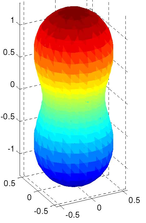
In this section, we present some numerical simulations of our proposed methods in sections 3 and 4. The models in our simulations are the unit sphere, the torus with inner radius 0.50.50.5 and outer radius 111, a dumbbell with the parametrization

𝐗(u,v)=(rsinvcosu,rsinvsinu,rcosv)𝐗𝑢𝑣matrix𝑟𝑣𝑢𝑟𝑣𝑢𝑟𝑣\mathbf{X}(u,v)=\begin{pmatrix}r\sin v\cos u,&r\sin v\sin u,&r\cos v\end{pmatrix} (67)

where r=0.92cos(2x)+10.94sin2(2x)𝑟superscript0.922𝑥1superscript0.94𝑠𝑖superscript𝑛22𝑥r=\sqrt{0.9^{2}\cos(2x)+\sqrt{1-0.9^{4}sin^{2}(2x)}}, see Figure 2, and a wave surface with

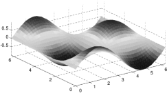
𝐗(u,v)=(u,v,sinucos(v)),𝐗𝑢𝑣matrix𝑢𝑣𝑢𝑣\mathbf{X}(u,v)=\begin{pmatrix}u,v,\sin u\cos(v)\end{pmatrix}, (68)

where (u,v)[0,2π]×[0,2π]𝑢𝑣02𝜋02𝜋(u,v)\in[0,2\pi]\times[0,2\pi], see Figure 3.

Refer to caption
Figure 2: The figure of a dumbbell
Refer to caption
Figure 3: The figure of the wave surface

5.1 Simulations for the O(r)𝑂𝑟O(r)-LTL algorithm

First, we show the numerical solutions of eigenvalues of Laplace-Beltrami operator on the unit sphere and some curved surfaces by the O(r)𝑂𝑟O(r)-LTL method in section 3.1. The O(r)𝑂𝑟O(r)-LTL approach is an special case for our O(rn)𝑂superscript𝑟𝑛O(r^{n})-LTL method. Although the O(r)𝑂𝑟O(r)-LTL method has a lower convergent rate, it only requires at least 5 neighboring vertices of each vertex on the surfaces and the triangular meshes always can be reconstructed such that the number of 111-ring neighboring vertices of each vertex is at least 555.

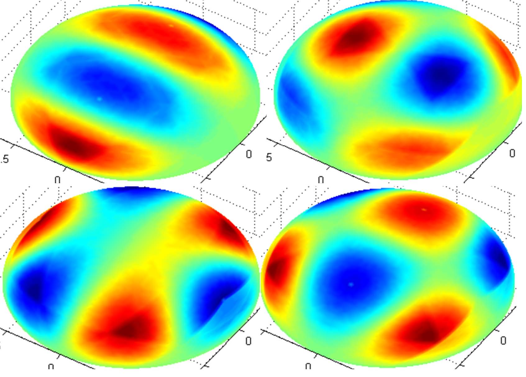
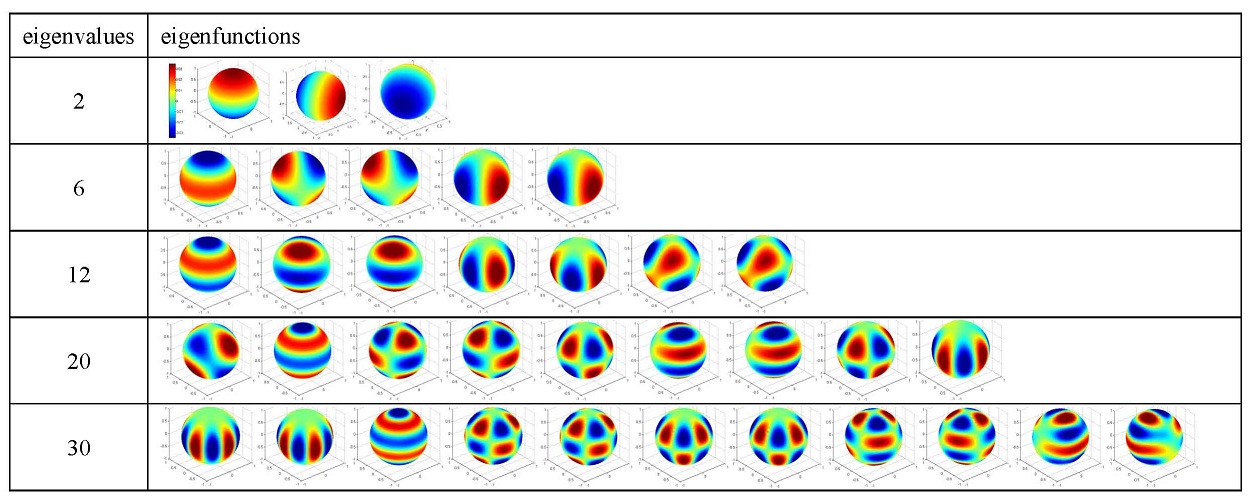
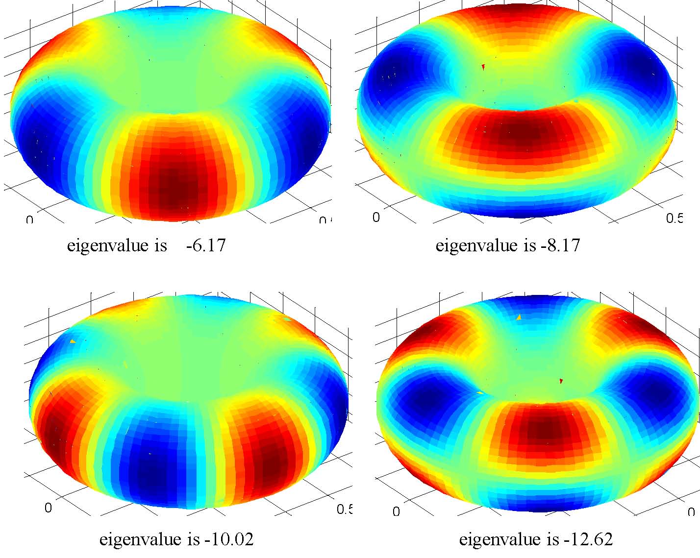
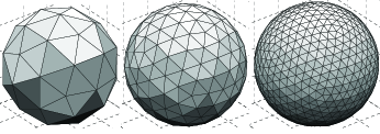
Table 1 shows the simulation results of the eigenvalues and its multiplicity of the Laplace-Beltrami operator on the unit sphere by our O(r)𝑂𝑟O(r)-LTL method. The triangular mesh sizes of the unit sphere in our simulations are 0.32,0.16,0.080.320.160.080.32,0.16,0.08 and 0.040.040.04. We give these triangular meshes in Figure 4. Figure 7 gives some eigenfunctions on the torus with inner radius 0.50.50.5 and outer radius 111 and Figure 6 shows all eigenfunctions corresponding to the first 5 eigenvalues on a unit sphere by the O(r)𝑂𝑟O(r)-LTL method.

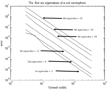
Figure 5 shows the convergence result of the eigenvalues of a unit hemisphere by our O(r)𝑂𝑟O(r)-LTL method. Our O(r)𝑂𝑟O(r)-LTL method has the quadratic convergence.
Refer to caption
Figure 4: The subdivision of triangular meshes of a unit sphere by O(r)𝑂𝑟O(r)-LTL method
Table 1: The eigenvalues and its multiplicity of a unit sphere
mesh size 1st eigenvalue 2nd eigenvalue 3th eigenvalue
(multiplicity) (multiplicity) (multiplicity)
0.32 -2.0484 (3) -6.0014 (5) -11.5986 (7)
0.16 -2.0117 (3) -6.0002 (5) -11,8998 (7)
0.08 -2.0029 (3) -6.0 (5) -11.9735 (7)
0.04 -2.0 (3) -6.0 (5) -12.0 (7)
Refer to caption
Refer to caption
Figure 5: The left shows some eigenfunctions of a hemisphere by O(r)𝑂𝑟O(r)-LTL method. The right is a convergence study for the first six eigenvalues of a unit hemisphere.
Refer to caption
Figure 6: The eigenfunctions of the Laplace-Beltrami operator on a unit sphere by O(r)𝑂𝑟O(r)-LTL method.
Refer to caption
Figure 7: The eigenfunctions of the Laplace-Beltrami operator on a torus by O(r)𝑂𝑟O(r)-LTL method.

5.2 Simulations for the O(rnO(r^{n})-LTL algorithm with n2𝑛2n\geq 2

In this subsection, we compute the Laplacian of a function,

F(u,v)=exp(0.5sinu+cos3v)𝐹𝑢𝑣0.5𝑢superscript3𝑣F(u,v)=\exp(0.5\sin u+\cos^{3}v) (69)

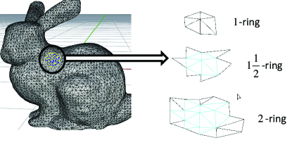
where (u,v)𝑢𝑣(u,v) defined on the domain of 𝐗(u,v)𝐗𝑢𝑣\mathbf{X}(u,v) in Equation (68), on the parametric surface in Equation (68) by high-order algorithms. How to determine the necessary neighboring vertices of a given vertex is an important problem for high-order accuracies. Ray et al.[15] proposed an elegant method to improve this problem by using the j2𝑗2\frac{j}{2}-ring (j2𝑗2j\geq 2) for neighboring vertices, see Figure 8. We will also use the j2𝑗2\frac{j}{2}-ring neighboring vertices in our simulations.

We estimate the lsuperscript𝑙l^{\infty} relative error of Laplacian on each mesh as

l relative error=max𝐯iV( relative error at 𝐯i)superscript𝑙 relative errorsubscriptsubscript𝐯𝑖𝑉 relative error at subscript𝐯𝑖l^{\infty}\mbox{ relative error}=\max_{\mathbf{v}_{i}\in V}(\mbox{ relative error at }\mathbf{v}_{i}) (70)

where

 relative error at 𝐯i= numerical solution at 𝐯i reference solution at 𝐯i reference solution at 𝐯i relative error at subscript𝐯𝑖norm numerical solution at subscript𝐯𝑖 reference solution at subscript𝐯𝑖norm reference solution at subscript𝐯𝑖\mbox{ relative error at }\mathbf{v}_{i}=\frac{\|\mbox{ numerical solution at }\mathbf{v}_{i}-\mbox{ reference solution at }\mathbf{v}_{i}\|}{\|\mbox{ reference solution at }\mathbf{v}_{i}\|} (71)

and  reference solution at 𝐯i0norm reference solution at subscript𝐯𝑖0\|\mbox{ reference solution at }\mathbf{v}_{i}\|\neq 0.

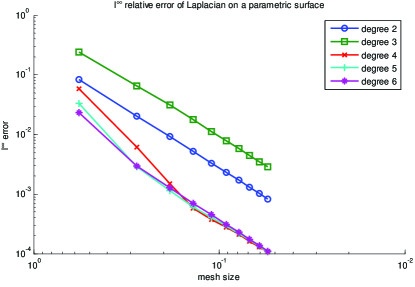
Figure 9 shows the lsuperscript𝑙l^{\infty} relative errors of Laplacian of the function F(u,v)=exp(0.5sinu+cos3v)𝐹𝑢𝑣0.5𝑢superscript3𝑣F(u,v)=\exp(0.5\sin u+\cos^{3}v) in the interior vertices on this parametric surface. These results always converge to the exact Laplacian when the mesh size of the triangular mesh approaches 00.

Refer to caption
Figure 8: The 111, 1121121\frac{1}{2} and 222-rings of a vertex on the bunny model.
Refer to caption
Figure 9: The lsuperscript𝑙l^{\infty} relative errors of laplacian of the function F(u,v)=exp(0.5sinu+cos2v)𝐹𝑢𝑣0.5𝑢superscript2𝑣F(u,v)=\exp(0.5\sin u+\cos^{2}v) in Equation on a wave surface in Equation (68)

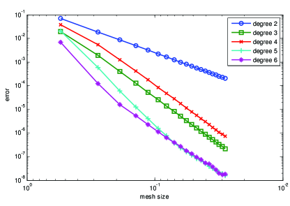
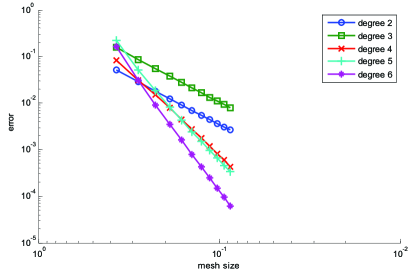
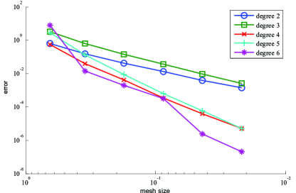
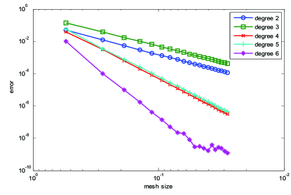
Now, we compare the eigenvalues and eigenfunctions on a unit sphere. It is well-known that the n𝑛n-th nonzero eigenvalues of the Laplace-Beltrami operator on the unit sphere are n(n+1)𝑛𝑛1-n(n+1) with multiplicity (2n+1)2𝑛1(2n+1). The eigenfunctions of the unit sphere are restrictions on the unit sphere of harmonic homogeneous polynomials in 3superscript3\mathbb{R}^{3}. Figures 10 and 11 show the errors of the eigenvalues λ=2𝜆2\lambda=2 and 666 on a unit sphere, repsectively. For the error e(h1)𝑒subscript1e(h_{1}) and e(h2)𝑒subscript2e(h_{2}) for the mesh size h1subscript1h_{1} and h2subscript2h_{2} the experimental error of convergence is defined as

EOC(h1,h2)=loge(h1)e(h2)(logh1h2)1.𝐸𝑂𝐶subscript1subscript2𝑒subscript1𝑒subscript2superscriptsubscript1subscript21EOC(h_{1},h_{2})=\log\frac{e(h_{1})}{e(h_{2})}\left(\log\frac{h_{1}}{h_{2}}\right)^{-1}. (72)

Tables 2 and 3 show the EOC of the first and second eigenvalues on the unit sphere, respectively.

Table 2: EOC of the 1st eigenvalue on a unit sphere
mesh size degree 2 degree 3 degree 4 degree 5 degree 6
0.5443 - - - - -
0.2774 2.0971 1.9543 3.6868 4.1610 6.7939
0.1877 2.0901 1.9751 4.1204 3.8777 5.9443
0.1407 2.0049 1.9327 4.0126 3.8251 6.1007
0.1130 2.0384 1.9872 4.0847 3.9515 6.2562
0.0941 1.9998 1.9626 4.0049 3.9122 5.9561
0.0807 2.0243 1.9949 4.0537 3.9847 6.9588
0.0706 1.9989 1.9754 3.9973 3.9468 5.8779
Table 3: EOC of the 2nd eigenvalue on a unit sphere
mesh size degree 2 degree 3 degree 4 degree 5 degree 6
0.5443 - - - - -
0.2774 1.8991 3.4314 2.8961 5.3251 5.9809
0.1877 2.0115 4.0060 3.7518 5.8448 5.2146
0.1407 1.9552 3.9231 3.7957 5.3624 3.8108
0.1130 1.9999 4.0148 3.9412 5.2539 3.8859
0.0941 1.9691 3.9537 3.9086 4.9920 3.7684
0.0807 1.9981 4.0113 3.9810 4.8949 3.7388
0.0706 1.9765 3.9473 3.9413 5.1215 3.6412

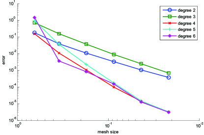
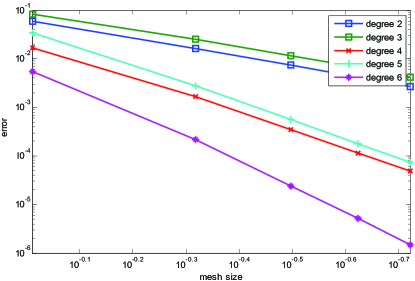
Let {ϕn,i}i=12n+1superscriptsubscriptsubscriptitalic-ϕ𝑛𝑖𝑖12𝑛1\{\phi_{n,i}\}_{i=1}^{2n+1} be the set of eigenfunctions corresponding to the eigenvalue n(n+1)𝑛𝑛1-n(n+1) on the unit sphere and let ϕ~n,isubscript~italic-ϕ𝑛𝑖\tilde{\phi}_{n,i} be the approximated solution by our O(rn)𝑂superscript𝑟𝑛O(r^{n})-LTL method. Then we choose ϕ¯n,isubscript¯italic-ϕ𝑛𝑖\bar{\phi}_{n,i} to be the linear combination i=12n+1αiϕn,isuperscriptsubscript𝑖12𝑛1subscript𝛼𝑖subscriptitalic-ϕ𝑛𝑖\sum_{i=1}^{2n+1}\alpha_{i}\phi_{n,i} so that it realizes the minimum of i=12n+1βjϕn,iϕ~n,inormsuperscriptsubscript𝑖12𝑛1subscript𝛽𝑗subscriptitalic-ϕ𝑛𝑖subscript~italic-ϕ𝑛𝑖\|\sum_{i=1}^{2n+1}\beta_{j}\phi_{n,i}-\tilde{\phi}_{n,i}\| over βjsubscript𝛽𝑗\beta_{j}’s. The error Ensubscript𝐸𝑛E_{n} of the nth eigenvalue with eigenfunctions ϕ¯n,isubscript¯italic-ϕ𝑛𝑖\bar{\phi}_{n,i} and the approximating eigenfunctions ϕ~n,isubscript~italic-ϕ𝑛𝑖\tilde{\phi}_{n,i} is defined by

En=supi{1,2,,2n+1}(ϕ¯n,iϕ~n,il).subscript𝐸𝑛subscriptsupremum𝑖122𝑛1subscriptnormsubscript¯italic-ϕ𝑛𝑖subscript~italic-ϕ𝑛𝑖superscript𝑙E_{n}=\sup_{i\in\{1,2,\cdots,2n+1\}}(\|\bar{\phi}_{n,i}-\tilde{\phi}_{n,i}\|_{l^{\infty}}). (73)

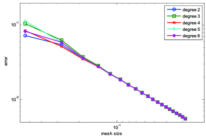
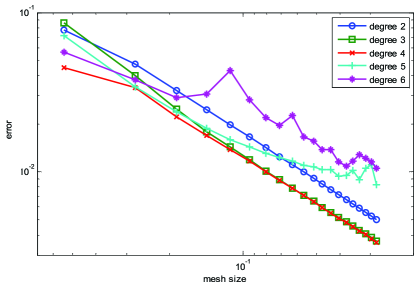
Figures 12 and 13 show the errors Ensubscript𝐸𝑛E_{n} in Equation (73) of the 1st and 2nd eigenvalues on a unit sphere, respectively.
Refer to caption
Figure 10: The errors of the 1st eigenvalues on a unit sphere.
Refer to caption
Figure 11: The lsuperscript𝑙l^{\infty} errors of the 2nd eigenvalues on a unit sphere.
Refer to caption
Figure 12: E1subscript𝐸1E_{1} on a unit sphere.
Refer to caption
Figure 13: E2subscript𝐸2E_{2} on a unit sphere.

5.3 Geometric invariants on curved surface

Finally, we estimate the normal vectors and the tensor of curvatures on regular surfaces. Figures 14 - 16 show the łsuperscriptitalic-ł\l^{\infty} relative errors of normal vectors, Gaussian curvatures and mean curvatures on a torus with the inner radius 0.50.50.5 and the outer radius 111. Figures 17 - 18 give the łsuperscriptitalic-ł\l^{\infty} relative errors of normal vectors, Gaussian curvatures and mean curvatures on a dumbbell in Equation (67) and Figure 19 shows the łsuperscriptitalic-ł\l^{\infty} errors of Gaussian curvatures on a wave surface. Obviously, the high-order algorithm is much more accurate than the low-order algorithm when the mesh size is small enough.
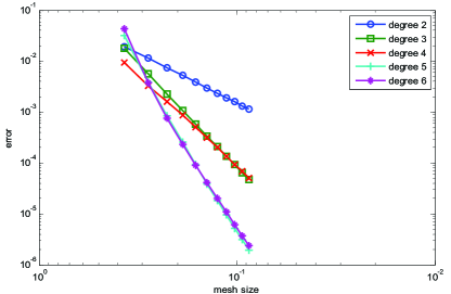
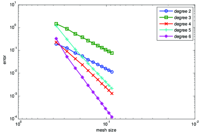
Refer to caption
Figure 14: The lsuperscript𝑙l^{\infty} relative errors of normal vectors on a torus
Refer to caption
Figure 15: The lsuperscript𝑙l^{\infty} relative error of Gaussian curvatures on a torus
Refer to caption
Figure 16: The lsuperscript𝑙l^{\infty} relative error of mean curvatures on a torus
Refer to caption
Figure 17: The lsuperscript𝑙l^{\infty} relative errors of Gaussian curvatures on a dumbbell
Refer to caption
Figure 18: The lsuperscript𝑙l^{\infty} relative error of mean curvatures on a dumbbell
Refer to caption
Figure 19: The lsuperscript𝑙l^{\infty} relative error of Gaussian curvatures on a wave surface

6 Dissusions and Conclusions

In 2012, Ray et al. also proposed a high-order numerical method for estimating the derivatives and integrations over discrete surfaces. Ray et al. solved the system of linear equations from Taylor expansion by the least square method. However, we deal with these problems from the viewpoint of duality and obtain our configuration equations for the Laplace-Beltrami operators over discrete surfaces. The configuration equation for Laplace-Beltrami operator is

(x1,x2,,xny1,y2,,ynx122,x222,,xn22x1y1x2y2,,xnyny122,y222,,yn22)(α1α2αn)=(00101)matrixsubscript𝑥1subscript𝑥2subscript𝑥𝑛subscript𝑦1subscript𝑦2subscript𝑦𝑛superscriptsubscript𝑥122superscriptsubscript𝑥222superscriptsubscript𝑥𝑛22subscript𝑥1subscript𝑦1subscript𝑥2subscript𝑦2subscript𝑥𝑛subscript𝑦𝑛superscriptsubscript𝑦122superscriptsubscript𝑦222superscriptsubscript𝑦𝑛22matrixsubscript𝛼1subscript𝛼2subscript𝛼𝑛matrix00101\begin{pmatrix}x_{1},&x_{2},&\cdots,&x_{n}\cr y_{1},&y_{2},&\cdots,&y_{n}\cr\frac{x_{1}^{2}}{2},&\frac{x_{2}^{2}}{2},&\cdots,&\frac{x_{n}^{2}}{2}\cr x_{1}y_{1}&x_{2}y_{2},&\cdots,&x_{n}y_{n}\cr\frac{y_{1}^{2}}{2},&\frac{y_{2}^{2}}{2},&\cdots,&\frac{y_{n}^{2}}{2}\end{pmatrix}\begin{pmatrix}\alpha_{1}\cr\alpha_{2}\cr\vdots\cr\alpha_{n}\end{pmatrix}=\begin{pmatrix}0\cr 0\cr 1\cr 0\cr 1\end{pmatrix} (74)

and the Laplacian Δf(0,0)Δ𝑓00\Delta f(0,0) in Equation (16) is given by

Δf(0,0)=i=1nαi(f(xi,yi)f(0,0)).Δ𝑓00superscriptsubscript𝑖1𝑛subscript𝛼𝑖𝑓subscript𝑥𝑖subscript𝑦𝑖𝑓00\Delta f(0,0)=\sum_{i=1}^{n}\alpha_{i}(f(x_{i},y_{i})-f(0,0)). (75)

Similarly, we can also obtain a high-order configuration equation for the Laplace-Beltrami operator in the O(rn)𝑂superscript𝑟𝑛O(r^{n})-LTL method.

Although the solution of the configuration equation may not be unique in general, the convergence rates of all solutions are similar by the theoretical analysis. However, not every solution has a good numerical simulation. Finding a suitable solution {αi}i=1nsuperscriptsubscriptsubscript𝛼𝑖𝑖1𝑛\{\alpha_{i}\}_{i=1}^{n} is a key problem in Ray’s method and our O(rn)𝑂superscript𝑟𝑛O(r^{n})-LTL methods. In Ray’s method, this problem can be improved by using the conditional number[15]. The pseudo inverse of the configuration matrix is a good approach to handle this problem in our O(rn)𝑂superscript𝑟𝑛O(r^{n})-LTL methods. Hence, we have

(α1α2αn)=pinv((x1,x2,,xny1,y2,,ynx1y1,x2y2,,xnynx12y12,x22y22,,xn2yn21,1,,1))(0000ϵ)matrixsubscript𝛼1subscript𝛼2subscript𝛼𝑛pinvmatrixsubscript𝑥1subscript𝑥2subscript𝑥𝑛subscript𝑦1subscript𝑦2subscript𝑦𝑛subscript𝑥1subscript𝑦1subscript𝑥2subscript𝑦2subscript𝑥𝑛subscript𝑦𝑛superscriptsubscript𝑥12superscriptsubscript𝑦12superscriptsubscript𝑥22superscriptsubscript𝑦22superscriptsubscript𝑥𝑛2superscriptsubscript𝑦𝑛2111matrix0000italic-ϵ\begin{pmatrix}\alpha_{1}\cr\alpha_{2}\cr\vdots\cr\alpha_{n}\end{pmatrix}=\mathrm{pinv}(\begin{pmatrix}x_{1},&x_{2},&\cdots,&x_{n}\cr y_{1},&y_{2},&\cdots,&y_{n}\cr x_{1}y_{1},&x_{2}y_{2},&\cdots,&x_{n}y_{n}\cr x_{1}^{2}-y_{1}^{2},&x_{2}^{2}y_{2}^{2},&\cdots,&x_{n}^{2}-y_{n}^{2}\cr 1,&1,&\cdots,&1\end{pmatrix})\begin{pmatrix}0\cr 0\cr 0\cr 0\cr\epsilon\end{pmatrix} (76)

in Equation (15) where pinv(𝐌)pinv𝐌\mathrm{pinv}(\mathbf{M}) is the pseudo inverse of the matrix 𝐌𝐌\mathbf{M}.

As expected, the high-order approach is more accurate than the low-order approach. However, the low-order approach is more stable than the high-order approach in our simulations. When we use the high-order approach, we need more neighboring vertices at each vertex and the structure of j2𝑗2\frac{j}{2}-ring becomes more complicated. For instance we need at least 26 neighboring vertices for the degree 666 approximations.

Note that our O(r)𝑂𝑟O(r)-LTL method is a special case of the O(rn)𝑂superscript𝑟𝑛O(r^{n})-LTL methods. In the O(r)𝑂𝑟O(r)-LTL method, we only need 555 neighboring vertices at each vertex for estimating the Laplacian of a function on a surface by the configuration equation (15). Almost all vertices on a closed triangular mesh can be reconstructed so that the number of 111-ring is at least 555 for each vertex in the new mesh. Ray’s method and our high-order configuration equation, Equation (74), need at least 666 neighboring vertices. Indeed, our O(r)𝑂𝑟O(r)-LTL method for estimating Laplacian is a generalization of the well-known the 555- point Laplacian method in 2superscript2\mathbb{R}^{2}.

In our O(r)𝑂𝑟O(r)-LTL configuration method, Equations (1) and (2) can be reduced to the matrix equations

(WA)(ϕ(V))=λ(ϕ(V))𝑊𝐴italic-ϕ𝑉𝜆italic-ϕ𝑉(WA)(\phi(V))=\lambda(\phi(V))

and

(WB)(ϕ(V))=λ(ϕ(V)),𝑊𝐵italic-ϕ𝑉𝜆italic-ϕ𝑉(WB)(\phi(V))=\lambda(\phi(V)),

respectively. The configuration masks A=(ai,k),B=(bi,k)formulae-sequence𝐴subscript𝑎𝑖𝑘𝐵subscript𝑏𝑖𝑘A=(a_{i,k}),B=(b_{i,k}) are given by

ai,k={αi,j if vk=vi,j,1 if i=k,0 otherwise,subscript𝑎𝑖𝑘casessubscript𝛼𝑖𝑗 if subscript𝑣𝑘subscript𝑣𝑖𝑗1 if 𝑖𝑘0 otherwise,a_{i,k}=\left\{\begin{array}[]{ll}\alpha_{i,j}&\mbox{ if }v_{k}=v_{i,j},\cr-1&\mbox{ if }i=k,\cr 0&\mbox{ otherwise,}\end{array}\right. (77)

and

bi,k={βi,j if vk=vi,j,1 if i=k,0 otherwise,subscript𝑏𝑖𝑘casessubscript𝛽𝑖𝑗 if subscript𝑣𝑘subscript𝑣𝑖𝑗1 if 𝑖𝑘0 otherwise,b_{i,k}=\left\{\begin{array}[]{ll}\beta_{i,j}&\mbox{ if }v_{k}=v_{i,j},\cr-1&\mbox{ if }i=k,\cr 0&\mbox{ otherwise,}\end{array}\right. (78)

where αi,jsubscript𝛼𝑖𝑗\alpha_{i,j} is a solution of Equation (15) and βi,jsubscript𝛽𝑖𝑗\beta_{i,j} is a solution of Equation (44). Using the configuration matrix A𝐴A, we can also solve the diffusion equation

utΔΣu=fsubscript𝑢𝑡subscriptΔΣ𝑢𝑓u_{t}-\Delta_{\Sigma}u=f

on regular surface ΣΣ\Sigma easily. Furthermore, our O(rn)𝑂superscript𝑟𝑛O(r^{n})-LTL configuration method can also solve general partial differential equations, L(u)=f𝐿𝑢𝑓L(u)=f, on a regular surface ΣΣ\Sigma or on more complicated domains, like Koch snowflakes. The key of our O(rn)𝑂superscript𝑟𝑛O(r^{n})-LTL configuration method for solving the PDE L(u)=f𝐿𝑢𝑓L(u)=f is to find the configuration matrix of the differential operator L𝐿L on the surface ΣΣ\Sigma.

It is worth to point out that our O(rn)𝑂superscript𝑟𝑛O(r^{n})-LTL configuration method is effective to solve the eigenpair problems with high-order accuracies even when the underlying surfaces or domains have complicated topological or geometrical structures.

In the near future, we shall extend our O(rn)𝑂superscript𝑟𝑛O(r^{n})-LTL configuration method to solve more partial differential equations on regular surfaces.

Acknowledgment

This paper is partially supported by NSC, Taiwan.

References

  • [1] S.-G. Chen, J.-Y. Wu, Estimating normal vectors and curvatures by centroid weights, Computer Aided Geometric Design 21 (2004) 447-458.
  • [2] S.-G. Chen, J.-Y. Wu, A geometric interpretation of weighted normal vectors and application, Proceeding of the IEEE Computer Society Conference on Computer Graphics, Imaging and Visualization, New Trends (2005) 422-425.
  • [3] S.-G. Chen, M.-H. Chi, J.-Y. Wu, Curvature estimation and curvature flow for digital curves, WSEAS transactions on computers 5 (2006)804-809.
  • [4] S.-G. Chen, M.-H. Chi, J.-Y. Wu, Boundary and interior derivatives estimation for 2D scattered data points, WSEAS transcations on computers 5 (2006) 824-829.
  • [5] S.-G. Chen, J.-Y. Wu, Discrete conservation laws on curved surfaces, SIAM Journal on Scientific Computing, 35(2) (2013) A719-A739.
  • [6] U. Clarenz, U. Diewald, M. Rumpf, Anisotropic geometric diffusion in surface processing, In Proceedings of Viz2000, IEEE Visualization, (2000) 397-405.
  • [7] M. Desbrun, M. Meyer, P. Schroder, A.H. Barr,Implicit fairing of irregular meshes using diffusion and curvature flow, SIGGRAPH99 (1999) 317-324.
  • [8] M. do Carmo, Differential Geometry of curves and surfaces, Prentice-Hall International, Inc., London, 1976.
  • [9] M. do Carmo, Riemannian Geometry, Birkhauser, Boston, 1992
  • [10] Colin B. Macdonald, Jeremy Brandman, and Steven J. Ruuth, Solving eigenvalue problems on curved surfaces using the Closest Point Method, Journal of Computational Physics 230 (2011) 7944-7956.
  • [11] M. Reuter, F.-E. Wolter, N. Peinecke, Laplace-spectra as fingerprints for shape matching, in: Proceedings of the 2005 ACM symposium on Solid and physical modeling, SPM 05 (2005)101-106.
  • [12] B. H. Romeny, Geometry driven diffusion in computer vision, Boston, MA, 1994.
  • [13] S. J. Ruuth, B. Merriman, A simple embedding method for solving partial differential equations on surfaces, Journal of Computational Physics, 227 (2008) 1943-1961.
  • [14] G. Kluwer Sapiro, Geometric partial differential equations and image analysis. Cambridge, University Press (2001).
  • [15] N. Ray, D. Wang, X.Jiao, and J. Glimm, High-order numerical integration over discrete surfaces, SIAM Journal on Numerical Analysis, 50(6) (2012) 3061-3083.
  • [16] Y. Shi, R. Lai, S. Krishna, N. Sicotte, I. Dinov, and A. W. Toga, Anisotropic Laplace-Beltrami eigenmaps: Bridging Reeb graphs and skeletons, in Proc. MMBIA (2008).
  • [17] Y. Shi, R. Lai, K. Kern, N. Sicotte, I. Dinov, and A. W. Toga, Harmonic surface mapping with Laplace-Beltrami eigenmaps, in Proc. MICCAI (2008).
  • [18] G. Strange and G. Fix, An analysis of the finite element method, Wellesley-Cambridge press 2nd edition, 2008.
  • [19] J.-Y. Wu, M.-H. Chi, and S.-G. Chen, A new intrinsic numerical method for PDE on surfaces, International Journal of Computer Mathematics, 89(1) (2012) 54-79.