On Demand Memory Specialization for Distributed Graph Databases

Abstract

In this paper, we propose the DN-tree that is a data structure to build lossy summaries of the frequent data access patterns of the queries in a distributed graph data management system. These compact representations allow us an efficient communication of the data structure in distributed systems. We exploit this data structure with a new Dynamic Data Partitioning strategy (DYDAP) that assigns the portions of the graph according to historical data access patterns, and guarantees a small network communication and a computational load balance in distributed graph queries. This method is able to adapt dynamically to new workloads and evolve when the query distribution changes. Our experiments show that DYDAP yields a throughput up to an order of magnitude higher than previous methods based on cache specialization, in a variety of scenarios, and the average response time of the system is divided by two.

1 Introduction

Graph databases have become quite popular over the last years. Social networks, bibliographic relations or metabolical pathways are some examples of datasets naturally expressed as graphs. In these scenarios, most computations that are performed against these datasets can be expressed as graph queries. For example, the home page of a social network, which shows the new posts of the users’ friends, can be implemented as a two hop traversal that navigates from the user to his friends and then to the published messages. Also, large analytical operations like finding the most influential users of a social network, can be implemented by computing the central users of the network with a sequence of breadth first search traversals of the graph [1].

The size of graph datasets is usually very large, and grows daily. For instance, in March 2011, Twitter users generated about a billion tweets per week [2], which corresponds to more than $1500$ tweets per second. As the size of the datasets increases, they become more and more difficult to manage on a single machine and graph partitioning becomes necessary. In addition, some environments require many queries answered per unit of time, making it also difficult for a single computer to cope with them. Graph partitioning is a common technique used to maintain data locality in distributed systems. Some systems partition the graph statically [3] but this requires computing the min cut of the graph, which is an NP-hard problem, and thus can be very expensive for some datasets. As a result, most of the current solutions, such as Pregel [4] or ParallelGDB [5], ignore this problem and partition the vertices by hashing their identifiers.

In this paper, we propose a dynamic approach, that we call DYDAP, for dynamic data partitioning, which is able to summarize the graph accesses through a compact data structure, that we call the DN-tree, for density tree. When a query is launched, the system analyzes the DN-tree contents and partitions the graph by taking into account the data access patterns of previous queries. Our approach does not compute the min cut of the whole graph, but only of a small graph induced by the DN-tree. Therefore, it ensures graph access locality while being scalable.

Our first contribution is the design of the DYDAP system for graph computation that divides the graph into small portions that have good locality properties based on the analysis of previous queries. Our approach distinguishes two levels: the secondary storage and the memory manager. The secondary storage is an independent persistent storage for the graph structure and its attributes. The memory manager specializes the memory of each node in the cluster and takes advantage of this cache specialization, allowing for faster query execution. The rest of our contributions are focused on the efficiency of the memory manager.

Our second contribution is the proposal and analysis of the DN-tree, a data structure that captures the sequence of data accesses. Since the amount of information can be very large, the DN-tree performs efficient compression, as analyzed in Section 6. The memory manager uses the DN-tree to analyze the data access patterns of ongoing queries, and is able to compute a new partitioning of the data at regular time intervals. Each new partitioning is based on the execution patterns of the queries that the system has executed until that point. This allows the system to adapt to varying workloads and improve the throughput of new queries. Other systems in the literature using similar partitioning schemes are static, meaning that the distribution of data is decided before starting the execution of queries and does not change during execution [5, 6]. These systems do not adapt to the nature of the incoming queries, and while they are optimized for some queries, if the incoming queries change, they are no longer optimal.

Our third and final contribution is to balance the load and network communication between nodes. The memory manager uses the information stored in the DN-tree data structure to compute a partitioning of the data that balances the load in each node while simultaneously balancing and minimizing the amount of network communication. As the experiments described in Section 7 show, this translates into an increased throughput of the queries executed and a decreased average response time, which is cut in half.

The rest of the paper is organized as follows: Section 2 formally defines the problem. Section 3 introduces a general vision of the DYDAP system. Section 4 describes the DN-tree data structure. Section 5 describes the partitioning strategy of our system. Section 6 analyzes the asymptotic size of the DN-tree structure and provides bounds on the error due to its compression. Section 7 describes the experiments and results obtained. Section 8 discusses related work. Section 9 concludes the paper.

2 Problem Definition

We assume a shared nothing cluster where data is divided into chunks of equal size, named extents, each of them with a unique identifier. An extent stores arbitrary data, and it is up to the database management system to decide how to store data in the extents. Due to the shared nothing architecture used, each node accesses a subset of the extents, and each pair of subsets is disjoint. Thus, there is a mapping between extents and nodes, that assigns a unique node to each extent. We call this mapping distribution function.

The execution of a query in the system is modeled as a Bulk Synchronous Processing (BSP) computation similar to that of the BFS algorithm in [7]. In this model, there are points in time where network communication is allowed, and intervals, named phases, where each node does computations on the data assigned to it according to the distribution function. The duration of each phase is determined by the slowest node, because all nodes need to finish their computations before network communication begins.

Our model assumes that the graph database can be updated, adding new vertices or edges. It also assumes that there are trends in the content searched by the queries and this pattern does not radically change over time. For example, a web server generating dynamic content issues similar queries although each query accesses a different set of the data. The model also assumes that there is no a priori knowledge about the queries that the system executes.

Our objective is to find an optimal distribution function, i.e. one that meets the following two objectives:

1. Minimize network communication.

2. Balance the load among the nodes during all computation phases.

The second objective focuses on load balancing. This balancing is twofold. On the one hand, the total workload for each node should ideally be the same; on the other hand, all nodes should always be performing useful computations. These two sides of load balancing are illustrated in the following example.

Example

Consider the following simplified example. The system consists of two nodes, labeled $n_{1}$ and $n_{2}$. The database consists of four extents, $\{e_{1},e_{2},e_{3},e_{4}\}$. We also assume that accessing the information on an extent and doing the required computations consumes one unit of time, and that exchanging through the network the information generated when accessing each extent costs one unit. There are two computational phases and one communication step in between.

A query $q$ accesses all extents, but $e_{1}$ and $e_{2}$ need to be accessed strictly before $e_{3}$ and $e_{4}$. A possible distribution function is one that maps $e_{1}$ and $e_{2}$ to $n_{1}$, and $e_{3}$ and $e_{4}$ to $n_{2}$. In the first phase, $n_{1}$ accesses $e_{1}$ and $e_{2}$, using 2 units of time while $n_{2}$ is idle. During the network communication phase, $n_{1}$ communicates the necessary information to $n_{2}$, using $2$ units of network cost. During the second phase, $n_{2}$ accesses $e_{3}$ and $e_{4}$ while $n_{1}$ is idle. The time consumed in the second phase is $2$ units, and the total cost is $4$ units of time plus $2$ units of network cost.

A second possible distribution function assigns $e_{1}$ and $e_{3}$ to $n_{1}$, and $e_{2}$ and $e_{4}$ to $n_{2}$. In the first phase, $n_{1}$ accesses $e_{1}$ and $n_{2}$ accesses $e_{2}$ in parallel, and the time consumed is one unit. Both nodes communicate through the network, using $2$ units of network cost, and similarly the second phase needs one unit of time, with $n_{1}$ accessing $e_{3}$ and $n_{2}$ accessing $e_{4}$. The total time is $2$ units of time plus $2$ units of network cost.

We note that both distribution function minimize network communication. However, only the second one balances the load. The first distribution function only balances the load globally, as both nodes have the same global amount of workload. The important difference is that the second distribution function parallelizes the computations.

2.1 Problem Formalization

In this section, we formalize the problem that we solve to obtain a distribution function, the Horizontal Multiconstraint Partitioning Problem (HMCPP) [8]. Let $G=(V,E)$ be a graph with $|V|=r$. A partitioning of $G$ in $k$ parts is a map $P:V\longrightarrow[0,k-1]$. Each vertex $v\in V$ belongs to partition $P(v)$. Given an edge $e\in E$ that joins two vertices $u,v\in V$, we say that $P$ cuts $e$ if $P(u)\neq P(v)$.

Each edge $e\in E$ has an associated scalar weight $w_{e}$, and each vertex $v\in V$ has an associated weight vector $w^{v}$ of size $m$. Each component of this vector is a balancing constraint, so there are $m$ constraints. Also, we assume, without loss of generality, that each constraint adds to $1$ when added along the whole graph, $\sum_{v\in V}{w_{i}^{v}}=1$, for $0\leq i<m$. The values of these constraints have to be balanced with respect to the partitions. Given $P$, a partitioning of $G$, we define the imbalance of constraint $i$ as

$$l_{i}=k\max_{0\leq j<k}\left(\sum_{v\in P^{-1}(j)}w_{i}^{v}\right)$$

for $0\leq i<m$. The imbalance is $k$ times the maximum value of the sum of the weights in each partition.

An optimal solution occurs when all constraints are balanced, i.e. $\sum{w_{i}}=\frac{1}{k}$ and thus $l_{i}$ is minimized, $l_{i}=1$. If a solution is not optimal, then $l_{i}>1$.

We define $c$ as a vector of size $m$, with $c_{i}\geq 1$. Each $c_{i}$ represents the maximum imbalance allowed for constraint $i$. Also, we define the edge cut as the sum of the weights of the edges cut by $P$, i.e. $\sum w_{e}$ for each vertex $e=(u,v)$ such that $P(u)\neq P(v)$.

The HMCPP is defined as: finding a partitioning $P$ of $G$ in $k$ parts that minimizes the edge cut, while $l_{i}\leq c_{i}$ for $0\leq i<m$. The solution that satisfies the HCMPP condition fulfills the previously presented objectives of network communication and load balance.

This problem is a well known NP-hard problem arising in several situations, for example VLSI circuit design [9] or detection of cliques in social, pathological and biological networks [10]. It has been extensively studied, and is solved by approximate algorithms very fast. One software that partitions graphs is METIS [8], which is the one we use.

3 DYDAP Overview

Figure 1: Overview of the distributed system.

Figure 1 shows the architecture of DYDAP, which logically separates the secondary storage (physical partitioning) from the memory manager in each node of the system.

The physical storage is used to store the data used by the system. Any physical storage able to store extents of fixed size indexed by a unique identifier can be used by the memory manager, which gives a useful decoupling between persistent storage and computation.

The memory manager distributes the data stored into the main memory of each node in an optimal way, according to the data analyzed during query execution. Each of the nodes that form the memory manager, four in Figure 1, contains three subsystems: the graph runtime, the query engine, and the partition manager.

The graph runtime is a graph database that is able to store locally a graph and execute graph operations. This database stores data in extents, and has to be modified to use the distributed storage as its permanent storage instead of the local hard disk. Additionally, it has to record accesses to extents and report them to the partition manager.

The partition manager monitors the accesses to the extents and stores the information in a DN-tree. At periodic intervals of time, the partition manager starts a repartition task in background and updates the distribution function. The first part of this repartition task is to gather and aggregate the DN-trees built in each node and merge them in a DN-tree of the full system, described in Section 4. The second part is the generation of the new distribution function as described in Section 5. During the repartition process, the queries can be executed using the last distribution function until a new one is computed. So, this process does not delay or interfere significantly with incoming queries.

Every time a new query enters the system, the query engine analyzes the data that the query accesses, and distributes it across the system, using the distribution function provided by the partition manager.

4 The DN-tree Data Structure

The partition manager captures the sequence of data accesses in the graph database and uses this information to improve its partitioning. The sequence of data accesses is recorded as a matrix of transitions, $M$, which in turn can be also viewed as a graph, where cell $M_{a,b}$ counts the number of times that extent $b$ has been accessed after $a$. If there are $m$ extents in the database, storing this information requires an $m\times m$ matrix, called $M$. This matrix can be used later to detect data access patterns that happen often in the system. For example, if the value of $M_{a,b}$ is large, then we will be able to improve the data access locality of the system by assigning extents $a$ and $b$ to the same node, because they are accessed often together. However, since the matrix $M$ can be very large, we propose an alternative data structure that approximates $M$, the density tree, or DN-tree. The DN-tree can be seen as a temperature map of the sequences of accesses to extents, which may be hot (often accessed) or cold (seldom accessed).

4.1 DN-tree Formalization

The DN-tree data structure consists of a rooted tree where each non-leaf vertex has exactly four children. Each vertex of the tree is associated with a subset of the matrix. The root vertex is associated with the whole matrix, and each of the four children of a vertex is associated to a spatial partitioning of the space in four equal quadrants. If a vertex of the tree monitors rows between $a$ and $b$, and columns between $c$ and $d$, we write this range as $[a,b]\times[c,d]$. For such a vertex, each of its four children monitors accesses to extents in the ranges

• $\left[a,\nicefrac{{(a+b)}}{{2}}\right]\times\left[c,\nicefrac{{(c+d)}}{{2}}\right]$

• $\left[a,\nicefrac{{(a+b)}}{{2}}\right]\times\left(\nicefrac{{(c+d)}}{{2}},d\right]$

• $\left(\nicefrac{{(a+b)}}{{2}},b\right]\times\left[c,\nicefrac{{(c+d)}}{{2}}\right]$

• $\left(\nicefrac{{(a+b)}}{{2}},b\right]\times\left(\nicefrac{{(c+d)}}{{2}},d\right]$

The root vertex is special and only contains pointers to its four children. The range of the matrix associated with the root vertex is $[0,m]\times[0,m]$ and thus the four subareas associated to its children are:

• $[0,m/2]\times[0,m/2]$

• $[0,m/2]\times(m/2,m]$

• $(m/2,m]\times[0,m/2]$

• $(m/2,m]\times(m/2,m]$

Each vertex different from the root vertex stores an integer that accounts for the number of accesses that the region associated has had.

Insertion:

First, we describe constructively the data structure. The insertion operations are inspired by quadtrees [11], as described in Algorithm 1. Initially, the DN-tree only contains the root vertex.

If extent $b$ is accessed after extent $a$, the value of the root child associated with the area containing $(a,b)$ is incremented in one unit. This happens every time accesses to different extents are done. This counter may reach a threshold value $\tau(i)=t\cdot k^{i}$, where $t$ and $k$ are constants (see Section 6 for a discussion on these values.) The parameter of $\tau$ is accounted by vertex.level in Algorithm 1 (the distance between the vertex and the root of the tree). For the root children, $\tau(1)=tk$. Once the counter reaches the threshold, the counter is not modified anymore and the DN-tree grows to record this area with more detail. Four new vertices are created, which are rooted on the saturated counter. Thereafter, the new vertices monitor the range of values of the saturated value, with the new counters initialized to zero. This is the source for the lossy nature of these data structure, as there is no way to know the distribution to the lower levels of the saturated counters. The method $selectChild$ returns a pointer to the child associated with the subarea where $(a,b)$ belongs to.

Algorithm 1 update(vertex, a, b)

0:  vertex: current vertex of the tree.

0:  a: previously accessed extent.

0:  b: last accessed extent.

1:  if vertex.value == $\tau(\mathrm{vertex.level})$ then

2:        let child = vertex.selectChild(a, b)

3:        update(child, a, b)

4:  else

5:        vertex.value = vertex.value + 1;

6:  end if

7:  return  

Query:

The DN-tree is used to compress a matrix $M$. Since the compression used is lossy, it is not possible to recover $M$, but an approximation $\hat{M}$. The DN-tree allows us to compute $\hat{M}(i,j)$, which is the value in row $i$ and column $j$ of $\hat{M}$, and it is an approximation of $M(i,j)$. The procedure to compute $\hat{M}(i,j)$ is a recursive traversal of the DN-tree from the root node to the leafs as shown in Algorithm 2, where value is initially $0$. For each vertex, we accumulate the counter corresponding to the subarea of $(i,j)$, and, in case it is not a leaf node, the counter is weighted by the number of accesses in that vertex. This procedure guarantees a reduced error as discussed in Section 6. In this algorithm, vertex.childSum stores the sum of the values of the four children of vertex.

Algorithm 2 density(vertex, a, b, value)

0:  vertex: current vertex of the tree.

0:  a: row extent.

0:  b: column extent.

0:  value: reference where the return value is stored.

1:  value = value + vertex.value;

2:  if vertex is not a leaf node then

3:        let w = vertex.selectChild(a, b)

4:        value = value * w.value / vertex.childSum

5:        density(w, a, b, value);

6:  end if

7:  return  

The DN-tree takes advantage of the query access patterns and the spatial locality of data structures in a graph database. In real databases, most transitions between extents seldom occur or will not occur at all. Thus, many sections of the matrix $M$ have a low density of accesses and can be effectively compressed by the DN-tree. The DN-tree works under the assumption that extents with close identifiers have similar access patterns. The DN-tree groups consecutive extents, forming bigger ranges of data.

(a) Density of $M$

(b) Density of $\hat{M}$

Figure 2: Density of $M$ and $\hat{M}$.

The areas with more extent accesses are more important, and thus the DN-tree data structure gives more detail than in areas with few or no accesses. As an example, Figure 2 shows the associated matrix obtained with a DN-tree along with the original uncompressed matrix that it approximates. The data is obtained by running $110$ breadth first search queries on a graph starting at a random vertex. The graph has about $45$ thousand vertices and $600$ thousand edges, and the resulting database has $512$ extents The matrix uses one MiB of memory while the DN-tree needs $138$ kiB, a compression ratio of $13\%$. During the execution of the queries, there are about $340$ million extent accesses. The figure shows that the original matrix and its approximation are very similar, and also that the cold regions dominate over the hot regions.

4.2 Distributed aggregation of DN-trees

In the DYDAP system, each node monitors its own activity, so the DN-tree only records the local accesses in each node. In order to aggregate the DN-trees, we use a tree-based scheme of communication to avoid bottlenecks. Each node receives the DN-tree from its two children, processes it, and passes it to its parent. The root node computes the next distribution function and passes it back to its children.

In order to send the DN-tree using the network, the DN-tree is serialized as the preorder list of the tree described. Along with the value of each vertex, there is a boolean, named marker, that stores false if the corresponding vertex has no children, and true otherwise.

Each node combines its own DN-tree with the ones it receives. The root node has the combination of all partial DN-trees. Since the communication scheme has a tree-form, in a cluster with $n$ nodes there are $n-1$ data exchanges.

Algorithm 3 shows how two serialized DN-trees are combined. This algorithm does one sequential read of each serialized DN-tree. The algorithm recursively walks over the arrays containing the serialized DN-trees, treating three cases: the first two cases correspond to when one of the DN-trees has a vertex in a branch that the other one does not. In this case, the value is directly copied from the DN-tree with the branch, and the next recursive call is executed if necessary. The third case corresponds to both DN-trees having the vertex in the branch. In this case, the values of the vertices are added and the next recursive call is executed as needed. We notice that during this process, some vertices in the resulting DN-tree may have a counter value higher than the threshold. Since the resulting DN-tree is only used by the partition manager to extract information and is not updated, this is not a source of problems.

Algorithm 3 join(src1, index1, src2, index2, ret)

0:  src1: array storing the first DN-tree.

0:  index1: integer that indexes src1. If its value is $-1$, src1 is assumed to be empty.

0:  src2: array storing the second DN-tree.

0:  index2: integer that indexes src2. If its value is $-1$, src2 is assumed to be empty.

0:  ret: array, initially empty, to store the result.

0:  The returned DN-tree ret is a compressed representation of the sum of the two matrices represented by the two DN-tree parameters.

1:  let mark1, mark2 be boolean values.

2:  for i from 1 to 4 do

3:        if index1 == -1 then

4:              ret.push_back(src2[index2++]);

5:              mark2 = src2[index2++];

6:              ret.push_back(mark2);

7:              if k != 0 then

8:                    join(src1, index1, src2, index2, ret);

9:              end if

10:        else if index2 == -1 then

11:              ret.push_back(src1[index1++]);

12:              mark1 = src1[index1++];

13:              ret.push_back(mark1);

14:              if k != 0 then

15:                    join(src1, index1, src2, index2, ret);

16:              end if

17:        else

18:              ret.push_back(src1[index1] + src2[index2]);

19:              index1++; index2++;

20:              mark1 = (src1[index1++] != 0);

21:              mark2 = (src2[index2++] != 0);

22:              ret.push_back(mark1 or mark2);

23:              if mark1 and mark2 then

24:                    join(src1, index1, src2, index2, ret);

25:              else if mark1 then

26:                    join(src1, index1, src2, -1, ret);

27:              else if mark2 then

28:                    join(src1, -1, src2, index2, ret);

29:              end if

30:        end if

31:  end for

32:  return  

5 Partition Manager

The partition manager provides a dynamic distribution function that changes over time depending on the queries executed and the load of each node. In this section, we describe the partitioning method used by the partition manager. Specifically, we describe how the Horizontal Multi-constraint Partitioning Problem maps to our system and how objectives $1$ and $2$, namely minimization of network communication and load balancing, described in Section 2, are achieved.

5.1 Partitioning Approach

In the graph $G$, each vertex is associated with an extent of the database. The edges are described by the adjacency matrix $\hat{M}$ obtained from the DN-tree as described in Section 4. Additionally, the value of $k$ is the number of nodes in our cluster. Thus, each of the partitions correspond to a node in the cluster.

Objective $1$ requires that the network communication is minimized. Given an edge that joins vertices $i$ and $j$, its associated weight, $M_{ij}$, is the number of times that extent $j$ has been accessed after $i$, it corresponds to the number of network messages exchanged when the nodes responsible for $i$ and $j$ are not the same. HMCPP minimizes the edge cut, which translates into the minimization of the amount of network communication. This is because edges between vertices belonging to the same partition involve no network communication, whereas edges between vertices belonging to different partitions do.

In order to comply with objective $2$, we define several weight constraints. The first constraint, $w_{0}$, is defined as $w_{0}^{v}=1$ for all $v\in V$. With this constraint, each subset is of a similar size and the total load of each node is balanced. As described in Section 2, the workload has to be parallelized. In order to accomplish this, we define more constraints, one for each data structure in the database whose extents can be accessed concurrently. Assuming there are $n_{\mathrm{DS}}$ different data structures, and naming $\mathrm{DS}_{i}$ the set of extents belonging to the data structure number $i$, we define $n_{\mathrm{DS}}$ additional constraints, for $1\leq i\leq n_{\mathrm{DS}}$:

$$w_{i}^{v}=\left\{\begin{array}[]{ll}1&\mbox{if }v\in\mathrm{DS}_{i}\\ 0&\mbox{if }v\notin\mathrm{DS}_{i}\end{array}\right.$$

The solution to HMCPP gives a logical partitioning that assigns a partition to each vertex. In DYDAP, this corresponds to assigning one node to each extent. This map from extents to nodes is the distribution function.

5.2 Example

In this section, we illustrate how the partition manager works. We consider a system with $2$ nodes and $4$ extents, numbered $0$ to $3$, and show how the DN-tree is constructed and used to partition the data.

Consider that during execution, the four extents of the system are accessed according to the following sequence:

{1, 2, 1, 3, 0, 1, 3, 1, 0, 1, 0, 2, $\mathrm{1}^{\diamond}$, 3, 1, 3, 0, 2, 1, 0, 2, 1, 3, 0, 3, 0, 1, 0, 1, 3, 1, 3, 1, 2, 0, 1, 3, 1, 3, 1, 2, 1, 2, 1}

This sequence is stored in a matrix $M$ as follows. Notice that we have marked the $5$ transitions from $0$ to $1$ in the input and the corresponding matrix entry $M_{0,1}$.

$$M=\left(\begin{matrix}0&\textbf{5}&3&1\\ 4&0&4&9\\ 1&6&0&0\\ 4&6&0&0\\ \end{matrix}\right)$$

We consider the sequence of accesses and see how the DN-tree is generated. Level $0$ of the DN-tree is the root node. It points to the four vertices in level $1$, represented in a $2\times 2$ matrix, with all four values set to $0$. The four quadrant correspond to different sets of extents, as shown in Figure 3. We set the parameters $t=4$, $k=1$ and start updating the DN-tree with each extent access. The first four accesses are $1$, $2$, $1$ and $3$, so the corresponding values are increased. The DN-tree is now as in Figure 3.

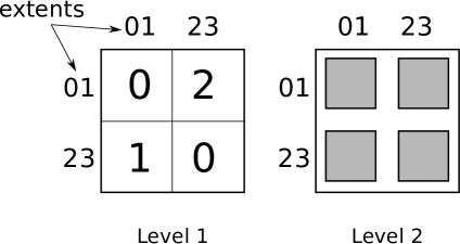
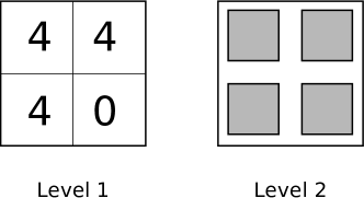
Figure 3: Evolution of the DN-tree.

After the first $13$ accesses, marked in the list with the diamond $\diamond$, the DN-tree is as shown in Figure 3. The next transition is from extent $1$ to $3$, which corresponds to position $(0,1)$, which has a value of $4$, the threshold value. Now, four new vertices are recursively generated and initialized. They will be modified during the following accesses. This is shown in Figure 3. After all $44$ accesses, three of the four vertices at level $1$ point to four other vertices each. This is represented in Figure 3.

The values $4$ and larger at level $2$ do not span new vertices because the extent range associated with these positions has size one and cannot be partitioned any further. In this example, the DN-tree is very small but not all branches have full depth. In real scenarios, branches have different depths.

An approximation of the real matrix $M$ is calculated with Algorithm 2. The resulting approximation is

$$\hat{M}=\left(\begin{matrix}0&5&3&1\\ 4&0&4&9\\ 1&5&0&0\\ 4&7&0&0\\ \end{matrix}\right)$$

Comparing the original matrix $M$ with the approximation $\hat{M}$, we see that only two values are different, and by one unit. In this small example, both $M$ and the DN-tree consist of $16$ integer values, and thus there is no compression. However, with large matrices the compression ratio is very large, as analyzed in Section 6.

Now, we calculate the optimal partitioning using both $M$ and its approximation $\hat{M}$. We consider the undirected graphs given by $M+M^{T}$ and $\hat{M}+\hat{M}^{T}$ as their adjacency matrix. As an example, the graph given by $M$ is represented in Figure 4. Its adjacency matrix is:

$$M+M^{T}=\left(\begin{matrix}0&9&4&5\\ 9&0&10&15\\ 4&10&0&0\\ 5&15&0&0\\ \end{matrix}\right)$$

Figure 4: Graph of network communication.

We partition the four vertices of the graph into two subsets of equal size. This leads to the different possible partitionings. Table 1 shows these partitionings along with their edge cut. Note that the edge cuts calculated with $\hat{M}$ are close to the real edge cuts obtained using $M$. The partitioning that minimizes the edge cut is the same in both cases. This partitioning minimizes the network communication between the two nodes. Note that the partitioning foundwith $\hat{M}$ is the same as the optimal partitioning that could be derived from $M$.

Partition 1	Partition 2	edge cut ($M$)	edge cut ($\hat{M}$)
{0, 1}	{2, 3}	34	34
{0, 2}	{1, 3}	24	23
{0, 3}	{1, 2}	28	29

Table 1: Partitionings and edge cuts with $M$ and $\hat{M}$.

6 DN-tree Analysis

In this section, we present a theoretical analysis of the properties of the DN-tree described in Section 4. Specifically, we analyze the asymptotic behavior of the memory needed to store the data structure, as well as an analysis of the error associated with the lossy nature of the compression.

6.1 Size Analysis

In this section, we give the asymptotic behavior of the size of the DN-tree as a function of the number of extent accesses, $N$. Assuming that the database has $m$ extents, the uncompressed matrix would need $O(m^{2})$ to be stored. We note that the asymptotic analysis assumes that both $m$ and $N$ tend to infinity. The number of accesses increases with time, but the number of extents also increases as new vertices and edges are added to the working dataset.

As described in Section 4, each level has an associated threshold. The first level, $0$, has a threshold value of $t$, and at each new level, the threshold is multiplied by a constant factor $k>1$. Thus, at level $r$, the threshold value is $tk^{r}$. We assume that each vertex of the DN-tree uses $1$ unit of memory to store its associated value.

One last assumption is that at each level, the accesses are distributed along the four children vertices following the same probability distribution: If we number the child nodes from $0$ to $3$, then the accesses are distributed following probabilities $p_{i}$, $0\leq i<4$, with $\sum_{i=0}^{3}p_{i}=1$. This means that the contents follow an R-MAT model [12].

We define a function $T(n,r)$ with two parameters: $n$, the number of extent accesses, and $r$, a level of the DN-tree. $T(n,r)$ gives the amount of memory necessary to store $n$ extent accesses starting at level $r$. Thus, the amount of memory used by a DN-tree storing $N$ extent accesses is $T(N,0)$.

The two parameters of $T$ allow to define a recurrence over $T$. Given $n$ and $r$, the base case is that $n$ is less than the threshold at level $r$, $n\leq tk^{r}$. If this is the case, the vertex at this level has no children and the amount of memory needed is $1$. If $n>tk^{r}$, then $tk^{r}$ is stored at level $r$, and the rest of the accesses, $n-tk^{r}$ are distributed to the four children at level $r+1$ following the probabilities $p_{i}$. Thus, the recurrence is defined as:

$$T(n,r)=\left\{\begin{array}[]{ll}1&\mbox{if }n\leq tk^{r}\\ 1+\sum_{i=0}^{3}T\left(p_{i}\left(n-tk^{r}\right),r+1\right)&\mbox{if }n>tk^{r}\end{array}\right.$$

In order to solve this recurrence, we first simplify it using the following lemma.

Lemma 6.1

$T(N,0)=T^{\prime}(N)$, where

$$T^{\prime}(n)=\left\{\begin{array}[]{ll}1&\mbox{if }n\leq t\\ 1+\sum_{i=0}^{3}T^{\prime}\left(p_{i}\frac{n-t}{k}\right)&\mbox{if }n>t\end{array}\right.$$

Proof 6.2.

We prove the following stronger statement, of which the lemma is a particular case:

$$T(n,r)=T^{\prime}\left(\frac{n}{k^{r}}\right)$$

The statement is proven using reverse induction. For every value of $n$, there is a value $r_{0}=\lceil\log_{k}\frac{n}{t}\rceil$, such that for all $r>r_{0}$, the statement is trivially true: $T(n,r)=T^{\prime}\left(\frac{n}{k^{r}}\right)=1$, since in both cases the base case condition is met.

Now, we prove that $T(n,r)=T^{\prime}\left(\frac{n}{k^{r}}\right)$ implies $T(n,r-1)=T^{\prime}\left(\frac{n}{k^{r-1}}\right)$:

$$T^{\prime}\left(\frac{n}{k^{r-1}}\right) = 1+\sum_{i=0}^{3}T^{\prime}\left(\frac{p_{i}}{k}\left(\frac{n}{k^{r-1}}-t\right)\right)$$

$$= 1+\sum_{i=0}^{3}T^{\prime}\left(\frac{p_{i}}{k^{r}}\left(n-tk^{r-1}\right)\right)$$

$$= 1+\sum_{i=0}^{3}T\left(p_{i}\left(n-tk^{r-1}\right),r\right)$$

$$= T(n,r-1)$$

Thus, for every $n$, $T(n,0)=T^{\prime}(n)$.

The new recurrence is interpreted as follows. Instead of increasing the threshold by a factor $k$, we maintain the threshold constant but reduce $n$ by the same factor in the recurrent call. With this, parameter $r$ is a constant and the new recurrence has only one parameter, which makes it easier to solve. Specifically, we observe that it can be solved using the Akra-Bazzi method (see Appendix A.) This method provides an analytical solution with a parameter $s$. Although we are not able to compute the exact value of $s$, we are able to use numerical methods and give a few bounds for the worst case in the following theorems.

Theorem 6.3.

The asymptotic space used by a DN-tree with parameters $k$ and $t$, is $T(N)\in\Theta\left(N^{s}\right)$, where $N$ is the number of extent accesses and $s$ is the solution to

$$\sum_{i=0}^{3}p_{i}^{s}=k^{s}$$

Proof 6.4.

We apply Akra-Bazzi theorem. Our recurrence has $g(n)=1$, $c=3$, $a_{i}=1$, $b_{i}=\frac{p_{i}}{k}$ and $h_{i}(n)=-\frac{p_{i}t}{k}$. It is easy to check that all conditions are met. In our case,

$$\int_{1}^{x}\frac{g(u)}{u^{s+1}}\,\mathrm{d}u=\int_{1}^{x}\frac{1}{u^{s+1}}\,\mathrm{d}u=s^{-1}\left(1-x^{-s}\right)$$

Thus, $T(N)\in\Theta\left(N^{s}\right)$, $\sum_{i=0}^{3}p_{i}^{s}=k^{s}$

We note that the asymptotic behavior does not depend on the value of $t$. Out of the two parameters needed to specify a DN-tree, $k$ and $t$, only $t$ has an effect on the asymptotic size of the DN-tree.

Theorem 6.5.

The asymptotic space used by a DN-tree with parameters $k\geq 1$ and $t$, is $T(N)\in\Theta\left(N^{s}\right)$, where $N$ is the number of extent accesses and $s$ is a real number between $0$ and $\frac{\log 4}{\log 4k}$.

Proof 6.6.

We define $f(s)=\sum_{i=0}^{3}p_{i}^{s}$. Using Lagrange multipliers and the Hessian matrix, it is easy to show that, fixing the value of $s$ and considering $p_{i}$ as variables, the value of $f(s)$ is maximized when $p_{i}=\frac{1}{4}$ for all $i$. This means that with $k$ fixed, The value of $s$ is maximized when all $p_{i}$ are equal. In this case, $s$ is explicitly calculated as $s=\frac{\log 4}{\log 4k}$.

Since the values of $p_{i}$ are fixed and are $0<p_{i}<1$, $f(s)$ is strictly monotonically decreasing. Also, using that $k^{s}$ is strictly monotonically increasing and $f(0)=4>k^{0}=1$ we conclude that the solution to $f(s)=k^{s}$ verifies $s>0$.

Corollary 6.7.

The asymptotic space used by a DN-tree with parameters $k\geq 1$ and $t$, is $T(N)\in\Theta\left(N^{s}\right)$, where $N$ is the number of extent accesses and $s$ is a real number between $0$ and $1$.

Proof 6.8.

$k\geq 1$ implies $\frac{\log 4}{\log 4k}\leq 1$

The size of the DN-tree is, in the worst case, sublinear in the number of extent accesses with a reasonable parametrization ($k>1$), as shown in Corollary 6.7. Moreover, Theorem 6.5 provides a tighter bound by a deep analysis of the worst case for $s$, which happens when the probability of all transitions recorded in the DN-tree is homogeneous.

Table 2 shows bounds found numerically for different values of $k$ and $p_{\mathrm{max}}=\max_{i\in\left[1,4\right]}{p_{i}}$ using Theorem 6.3. When $p_{\mathrm{max}}=0.25$, the bound is that given by Lemma 6.5. Other cases are, for example, $p_{\mathrm{max}}=0.9$ and $k=2$, where the DN-tree has size $O\left(N^{0.52}\right)$, while with $k=8$ the size is $O\left(N^{0.32}\right)$. This corresponds approximately to the square and third roots of $N$, respectively. With one MiB of memory, these configurations store about $10^{12}$ and $10^{18}$ extent accesses, respectively.

k	1.5	2	4	8
size	$O\left(N^{0.77}\right)$	$O\left(N^{\frac{2}{3}}\right)$	$O\left(N^{\frac{1}{2}}\right)$	$O\left(N^{\frac{2}{5}}\right)$

Table 2: Bounds for size of the DN-tree.

$p_{\mathrm{max}}/k$	1.5	2	4	8
0.25	0.77	0.67	0.50	0.40
0.3	0.77	0.67	0.50	0.40
0.4	0.77	0.66	0.50	0.40
0.5	0.76	0.65	0.49	0.39
0.6	0.74	0.64	0.48	0.38
0.7	0.72	0.61	0.46	0.37
0.8	0.69	0.58	0.44	0.35
0.9	0.63	0.53	0.40	0.32

Table 3: Exponent for the size of the DN-tree.

The configuration parameter $k$ allows fine control over the growth of the DN-tree. Table 3 summarizes values of $s$ for different values of $k$ and distributions of data. However, the growth of the DN-tree can be controlled further. One of the assumptions in Section 2 is that queries follow some common pattern and do not change radically over time. This means that after some time, we can simply stop updating the DN-tree, as the behavior of the queries has already been captured. This is especially useful in environments with heavy loads and lots of data accesses, because both the CPU and memory usage are reduced.

6.2 Error Analysis

(a) {0.30, 0.25, 0.25, 0.20}

(b) {0.45, 0.25, 0.25, 0.05}

(c) {0.9, 0.09, 0.009, 0.001}

Figure 5: Error for different configurations with $N=10^{9}$.

The compression used to store the matrix is lossy, meaning that we are not able to recover exactly the original matrix but an approximation. In this section, we give bounds for the error due to the compression.

We take the same assumptions as in Section 6.1: the matrix contents follow an R-MAT pattern defined by the four probabilities $p_{0}$, $p_{1}$, $p_{2}$ and $p_{3}$. Given a matrix $M$ and an approximation $\hat{M}$, we calculate the error as the sum of the absolute value of all the elements of $M-\hat{M}$.

We have considered different configurations and generated matrices corresponding to different values of the number of extent accesses, $N$. We compare the matrix generated by our data structure, $\hat{M}=\left(\hat{m}_{ij}\right)$, with the original matrix, $M=\left(m_{ij}\right)$, and the error is computed as:

$$\mbox{error}=\frac{1}{2\left(N-1\right)}\sum_{i,j}\left|m_{ij}-\hat{m}_{ij}\right|$$

Since the sum of the elements of both matrices is identical and equal to $N-1$, the factor $2\left(N-1\right)$ ensures that the error value is between zero and one.

Figure 5 shows graphs for three different configurations of the values of $p_{i}$. The vertical axis corresponds to the error while the horizontal axis represents the threshold growing constant $k$. Each graph has three plots, corresponding to three different sizes of matrix $M$, $512\times 512$, $2048\times 2048$ and $8192\times 8192$, representing datasets with $512$, $2048$ and $8192$ extents.

The first graph, in Figure 5(a), corresponds to values of $p_{i}$ equal to {$0.30$, $0.25$, $0.25$, $0.20$}, which is very close to the uniform distribution $p_{i}=0.25$. With this distribution, the error is small for all values of $k$. The graph in Figure 5(c) corresponds to values of $p_{i}$ equal to {$0.9$, $0.09$, $0.009$, $0.001$}, which is a very different distribution and the error is higher. Figure 5(b) corresponds to a distribution between the other two, and the error is significantly higher than the one in Figure 5(a), but does not grow as high as the one in Figure 5(c).

We observe that for all configurations, a small value of $k$ is associated with a small error. This is in contrast to the size analysis, where small values of $k$ are associated with larger sizes of the data structure. For our experiments, we choose a value of $k=1.5$, which provides a very small error, and experiments show that the data structure uses less than $0.2\%$ of the available memory of the system and it represents less than $0.002\%$ of the size of the full matrix $M$.

7 Experimental Evaluation

We ran experiments with the DYDAP system using two different datasets. The first dataset is a synthetic R-MAT graph [12], while the second one is a graph built with information from Twitter. The first dataset is used with a query that accesses all vertices and edges of the graph, and is used to measure the throughput of the system. The Twitter dataset is used with queries that generally access a small fraction of the database, and is useful to evaluate the average response time of the system, as it is necessary that these types of queries execute in a very short time.

Our proposal is compared to a state-of-the-art static partitioning method, used in ParallelGDB [5], which we use as baseline. This method statically defines a fixed distribution function that does not adapt to incoming queries.

7.1 Prototype Implementation

In the experiments, we use an implementation of the complete system as described in this paper, using a modified version of DEX 4.2 [13] as the graph runtime. DEX is used to execute the queries at each node. The system supports an arbitrary number of nodes, and uses MPI for data communication between them. The distributed file system is the same used by ParallelGDB, described in [5].

The execution of a query follows the model described in Section 2. Once the query is finished, there is a final round of network communication where all nodes send information to the node that started the query, which outputs the result.

7.2 Synthetic Data

The synthetic dataset is used to measure throughput, as well as the standard deviation of the load and network communication of the nodes. The query executed accesses the whole graph, and is used to simulate analytic scenarios where queries explore a large portion of the database.

The throughput is measured in traversed edges per second (TEPS.) This unit describes the amount of graph edges that the system processes each second while executing a query.

We also report the standard deviation of the amount of load and network communication. Since the standard deviation has the same units as the data, its units are the number of traversed vertices and bytes, respectively.

Setup

The graph used is the biggest connected component of an R-MAT graph [12] with $2^{26}$ vertices and mean degree $16$. The resulting graph has more than $37$ million vertices and one billion edges ($37,165,451$ and $1,051,580,953$, respectively).

The query executed on the R-MAT graph is a BFS starting from a randomly selected fixed vertex. The query accesses the whole graph, and exhibits poor locality, as data is not accessed repeatedly. It is executed using $10$ BSP phases. Each phase calculates the next hop using as a source the new vertices explored in the previous phase, and the load and network communication is recorded at each node.

The BFS query is executed in a cluster with identical nodes, with 2x AMD Opteron 6164 HE CPUs running at $1.7$ GHz and with $48$ GiB of RAM. The nodes run a Linux base OS with kernel version $2.6.32$. The graph engine is configured to use a maximum of $16$ GiB of RAM and to run using only one core of the $12$ available.

Additionally, the memory of the nodes is cleared before the first execution of each configuration. The BFS query is executed twice, without clearing the memory between the two executions. The results are reported as $\mathrm{static}_{1}$, $\mathrm{static}_{2}$, $\mathrm{DYDAP}_{1}$ and $\mathrm{DYDAP}_{2}$ where the subindex indicates whether it corresponds to the first or second execution.

With this setup, the DN-tree uses a maximum of $27.2$ MiB on each node, which is $0.16\%$ of available memory.

Throughput

Figure 6: Throughput of a BFS.

system / #nodes	1	2	8	32
(1) static1	38,180	29,425	34,427	48,031
(2) static2	-	-	-	59,061
(3) DYDAP1	38,180	54,881	114,389	151,198
(4) DYDAP2	-	63,310	194,882	525,790
Speedup (3)/(1)	1	1.9	3.3	3.1
Speedup (4)/(3)	-	1.2	1.7	3.5
Speedup (4)/(2)	-	-	-	8.9
Speedup (4)/(1)	-	2.3	5.6	10.9

Table 4: Throughput in TEPS and speedups.

Table 4 and Figure 6 show the throughput in TEPS of the BFS query both for the static method and our proposal in clusters with $2$, $8$ and $32$ nodes. The graph also shows a second execution of the query in DYDAP for all configurations and a second execution of the static method with $32$ nodes. The differences in the first execution are due to the load balancing, and the improvements of the second executions are due to the use of the cache of the computers.

With one node, the result is independent of the system, as no distribution takes place, and corresponds to executing the regular graph manager; in this case the regular version of DEX, modified to communicate with the partition manager.

When executed using two nodes, the baseline explores $29,425$ edges per second. The execution of the query using the static method is used to collect data to partition the database according to this query load and generate the first distribution function for our method. When the query is executed using DYDAP, it achieves $54,881$ TEPS, or $87\%$ better throughput.

Using eight nodes, the baseline traverses $34,427$ edges per second, while DYDAP explores $114,389$. In this case, the throughput of DYDAP is $3.3$ times that of the baseline, and more than twice the throughput of DYDAP with two nodes. A second execution achieves a throughput of $194,882$ TEPS, which is $70\%$ more than the throughput of the first execution.

With $32$ nodes, the query is executed two times on each system. The static method explores $48,031$ edges per second during the first execution and $59,061$ during the second one. This improvement of $23\%$ in throughput is due to the cache specialization. Our system performs its first execution with a throughput of $151,198$ TEPS, which is $3.15$ times the throughput of the first execution with the static method. The second execution achieves $525,790$ TEPS, which is almost an order of magnitude faster than the baseline.

Load

The results of the following two subsections show how our system balances the load and network communication between nodes, allowing the improvement seen in the first execution of the query. The further improvement on the second execution over the first one shows that our system is better at doing the cache specialization of the nodes.

(a) $2$ nodes.

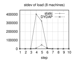
(b) $8$ nodes.

(c) $32$ nodes.

(d) $2$ nodes.

(e) $8$ nodes.

(f) $32$ nodes.

Figure 7: Standard deviation of load (top) and network communication (bottom) at each phase.

For the configuration with two nodes, Figure 7(a) shows the standard deviation of the load of both nodes at each phase, measured as the number of vertices traversed, using the static method and our proposal. Notice how at each step, the load at each node is almost identical using our proposal, while there are differences using the static method. This differences imply that one node is idly waiting for the other to finish, in order to start the network communication. This accounts for the time saved when using our system.

Figures 7(b) and 7(c) show the standard deviation of the load when using $8$ and $32$ nodes for both methods. Here we observe how the standard deviation is much lower for our method, which means that all nodes have a similar load, drastically reducing the time needed to finish the query.

Network Communication

Using two nodes, Figure 7(d) shows the standard deviation of incoming network communication between each pair of consecutive phases for one of the two nodes. Since there are only two nodes in the system, it is equivalent to the standard deviation of outgoing network communication. We observe that the distribution of network communication is uneven with the static method, but almost equal in DYDAP. This is a side effect of having a balanced load.

Figures 7(e) and 7(f) show the standard deviation of incoming network communication for the systems with $8$ and $32$ nodes. In these cases it is also clear that network communication is much more balanced in our proposal than in the baseline, which means that it completes much faster.

7.3 Real Data

The query on the Twitter dataset is used to compute the average response time of the system. The query executed on this dataset explores a small portion of the graph, and simulates scenarios such as web servers, where there are a large number of queries and each query does not access a large fraction of the database. The average response time of the system is measured in seconds, and is calculated as the duration of a time frame divided by the number of queries that the system executes during that time frame.

Setup

The Twitter dataset is generated by combining the data obtained from [14] and [15], it contains over $40$ million users, $26$ million tweets and one billion following/follower relationships. This graph has four different types of vertices: user, tweet, hashtag and url; and seven types of edges: tweets, follows, receives, depicts, retweet, tags and reference. Each edge type joins two specific vertex types, for example, a tweets edge joins a user vertex with a tweet vertex. The database with all the information has a size of 248 GiB.

The query executed on this dataset is a 2-hop. It simulates the generation of the home page of a user. Given $u$, a vertex of type User, the first hop explores the edges of type follows that start at $u$. After this step, the query has a set of vertices of type User that $u$ follows. The second hop expands this set through edges of type tweets. This second hop is done through a different edge type; this means that a different data structure is accessed. The final results are the tweets of the users that $u$ follows. This is an example of a system issuing queries interactively to generate web pages in real time. Thus, it is very important to have low response times.

The 2-hop query has been executed on Amazon EC2. The instances used are of type m2.xlarge: $17.1$ GiB of memory and $6.5$ EC2 Compute Units ($2$ virtual cores with $3.25$ EC2 Compute Units each). The database is stored using an EBS volume for each instance. Also, the graph engine is configured to use a maximum of $12$ GiB of memory.

With this setup, the DN-tree uses a maximum of $7.5$ MiB on each node, which is $0.06\%$ of available memory.

Average response time

On each system, the query is executed multiple times using a random vertex of type User as a parameter. Each node has $10$ threads executing queries concurrently during $90$ minutes. The results reported are the average response time of the system for the last $30$ minutes, which is calculated as the time elapsed divided by the number of queries executed. The whole experiment is executed three times and the best results for each configuration are reported.

Figure 8: Average response time for 2-hops during the last $30$ minutes of execution.

Figure 8 shows the average response time for both methods for configurations with $2$, $4$ and $8$ nodes. With $2$ nodes, the average response time of our system is $67.9\%$ of that of the baseline. For $4$ and $8$ nodes, our average response time is reduced to $40.1\%$ and $45.6\%$ with respect to the baseline.

We observe that, with four nodes, the average response time is divided by two. Using eight nodes does not improve the response time by a large factor because, on average, the queries do not require a lot of computation, which means that the network costs are a large fraction of the total cost.

7.4 Summary

The experiments performed using synthetic data show that our system scales with the number of nodes, and our dynamic data partitioning outperforms a state of the art static method by a factor of three during the first execution. During the second execution, when the system is warmed up, the baseline barely improves, while DYDAP achieves a throughput an order of magnitude larger than that of the baseline. This is because our system is better at performing node cache specialization. Also, analyzing the load and network usage of each node, we see that it is much more balanced in DYDAP, which allows a much better performance.

The experiments with real data show that DYDAP has an average response time that is less than half of the baseline when using at least four nodes. We see that with four nodes, DYDAP already achieves a very good result, with an average response time of $12$ ms. With eight nodes, the average response time is similar, $10$ ms. This is due to the fact that this query is relatively simple, so the time spent in network communication during the query dominates with respect to the time spent accessing the data to answer the query when the number of nodes is large. Our system uses all the available nodes to solve each query. We leave as future work to analyze the compromise between the resources dedicated to solve each query and the response time of the system.

8 Related Work

There are descriptions of several distributed systems in the literature. The majority of them work with relational or key-value models, but some of them employ a graph model. In this section, we review some of the distributed systems that work with graphs and also discuss generic approaches that are applied both to graph and non-graph models.

MapReduce has become in the latest years the main paradigm for processing large batches of embarrassingly parallel tasks. Graph mining tasks such as calculating the diameter of the graph or the connected components can be computed using MapReduce. For example, Pegasus [16] is a library that represents the graphs as a sparse matrices, which are loaded in a MapReduce platform. These matrices can be manipulated with sequences of algebraic operations that simulate graph mining operations such as calculating the diameter of a graph or the connected components. However, these systems do not take into account locality decisions and are not suitable for obtaining fast results from queries because of the overheads associated to start MapReduce tasks. In [17], the authors present an analysis of MapReduce techniques to perform graph operations and conclude that MapReduce has severe limitations. The communication between processes is a bottleneck, as the programs need to exchange a large amount of data. Although some limitations are inherent to the nature of graph data, the solution presented in our paper could be implemented in MapReduce platforms to improve its efficiency.

Google proposed a framework for efficient graph processing called Pregel [4] as an alternative to MapReduce. Pregel defines a message communication network among the vertices that uses the edges as connections. Graph algorithms are programmed as sequences of message exchanges in this network. Other papers by different authors improve Pregel. For example, Sedge [3] adds the management of different partitions over the original graph, and in [18] the authors propose a method that changes the partitioning by exploring the behavior of the system during a working window. PowerGraph [19] is a distributed system using a model very similar to that of Pregel, but partitions vertices instead of edges. Although Pregel alleviates the network bottlenecks of MapReduce, this solution is also oriented to large scale graph mining and not queries with short response time. Besides, it requires rewriting all graph algorithms in terms of such network communication model, which is not close to the traditional graph abstract data type. In contrast, we use a traditional API programming model that allows the use of classic implementations of graph algorithms.

One method used to improve system throughput is cache specialization, which ensures data locality. In [20], the authors present a load balancing method for relational databases that assigns transactions to replicas in a way that they are executed in memory, thus reducing disk usage. This method is an example of system using data locality. Our system is different because it does not use replicas, but rather distributes the only copy of the data between nodes, also exploiting data locality to reduce disk usage.

In [21], the authors propose a method for partitioning and replication of social networks that minimizes the number of replicas necessary to guarantee data locality for all vertices. A generalization of this method is presented in [22]. These two methods focus on controlling the number of replicas to minimize network communication. Our method does not replicate data and additionally balances the load of the computers. Also, these methods require an expensive process of recomputing partitionings when the graph is modified, while our partitioning recomputations are very fast.

ParallelGDB [5] is a static method to distribute a graph database that works by specializing the caches of the nodes in the system, reducing disk and network I/O. Our method works similarly, but the partitioning is adapted to the incoming queries, and provides high performance also in cases where the workload is skewed.

Schism [6, 23] is an approach to relational database partitioning and replication that uses a method similar to ours to partition data. The method constructs a graph that assigns one vertex to each tuple of the database. The resulting graph is often very large and it has to be sampled to improve efficiency, while our system does not use sampling. A limitation of this method is that it needs to know the query workload before execution starts, and what data each query accesses, instead of adapting to incoming queries.

9 Conclusions

In this paper, we proposed a distributed system design in two levels: secondary storage and memory manager. Independently of the storage implementation used, the memory manager specializes the cache of the computing nodes. The memory manager uses a new method to dynamically partition data in a graph database. This data partitioning balances the load and minimizes the amount of network communication in the distributed system. The goal is to adapt the data partitioning to the incoming query workload, and this goal is achieved as shown by the experiments.

Our experimental results show that our distributed system works in a variety of different situations. It provides great performance when used to analyze huge amounts of data, and also in a web environment, where queries are simpler but require a very short response time.

Appendix A Akra-Bazzi theorem

Theorem A.1 (Akra-Bazzi [24]).

Given a recurrence of the form:

$$T(n)=g(n)+\sum_{i=0}^{c}a_{i}T(b_{i}n+h_{i}(n))$$

with the following conditions: $a_{i}$ and $b_{i}$ are constants; $a_{i}>0$; $0<b_{i}<1$; $|g(n)|\in O\left(n^{d}\right)$, where $d$ is a constant; and, $|h(n)|\in O\left(\nicefrac{{n}}{{\left(\log n\right)^{2}}}\right)$.

The asymptotic behavior of $T(n)$ is given by:

$$T(n)\in\Theta\left(n^{s}\left(1+\int_{1}^{n}\frac{g(u)}{u^{s+1}}du\right)\right)$$

where $s$ is the solution to the equation:

$$\sum_{i=0}^{c}a_{i}b_{i}^{s}=1$$

References

- [1] U. Brandes, “A faster algorithm for betweenness centrality,” J. of Mathematical Sociology, vol. 25, no. 2, pp. 163–177, 2001.
- [2] ”http://blog.twitter.com/2011/03/numbers.html”.
- [3] S. Yang, X. Yan, B. Zong, and A. Khan, “Towards effective partition management for large graphs,” in SIGMOD Conference, 2012, pp. 517–528.
- [4] G. Malewicz, M. H. Austern, A. J. C. Bik, J. C. Dehnert, I. Horn, N. Leiser, and G. Czajkowski, “Pregel: a system for large-scale graph processing,” in SIGMOD Conference, 2010, pp. 135–146.
- [5] L. Barguñó, V. Muntés-Mulero, D. Dominguez-Sal, and P. Valduriez, “ParallelGDB: a parallel graph database based on cache specialization,” in IDEAS, 2011, pp. 162–169.
- [6] C. Curino, Y. Zhang, E. P. C. Jones, and S. Madden, “Schism: a workload-driven approach to database replication and partitioning,” PVLDB, vol. 3, no. 1, pp. 48–57, 2010.
- [7] A. Yoo, E. Chow, K. W. Henderson, W. M. III, B. Hendrickson, and Ü. V. Çatalyürek, “A scalable distributed parallel breadth-first search algorithm on bluegene/l,” in SC, 2005, p. 25.
- [8] G. Karypis and V. Kumar, “Multilevel algorithms for multi-constraint graph partitioning,” in SC, 1998, p. 28.
- [9] K. Andreev and H. Räcke, “Balanced graph partitioning,” Theory Comput. Syst., vol. 39, no. 6, pp. 929–939, 2006.
- [10] S. B. Patkar and H. Narayanan, “An efficient practical heuristic for good ratio-cut partitioning,” in VLSI Design, 2003, pp. 64–69.
- [11] R. A. Finkel and J. L. Bentley, “Quad trees: A data structure for retrieval on composite keys,” Acta Inf., vol. 4, pp. 1–9, 1974.
- [12] D. Chakrabarti, Y. Zhan, and C. Faloutsos, “R-mat: A recursive model for graph mining,” in SDM, 2004.
- [13] N. Martínez-Bazan, M. Águila-Lorente, V. Muntés-Mulero, D. Dominguez-Sal, S. Gómez-Villamor, and J. Larriba-Pey, “Efficient graph management based on bitmap indices,” in IDEAS, 2012, pp. 110–119.
- [14] ”http://snap.stanford.edu/data/bigdata/twitter7/”.
- [15] ”http://an.kaist.ac.kr/traces/WWW2010.html”.
- [16] U. Kang, C. E. Tsourakakis, and C. Faloutsos, “Pegasus: mining peta-scale graphs,” Knowl. Inf. Syst., vol. 27, no. 2, pp. 303–325, 2011.
- [17] J. Cohen, “Graph twiddling in a mapreduce world,” Computing in Science and Engineering, vol. 11, no. 4, pp. 29–41, 2009.
- [18] Z. Shang and J. X. Yu, “Catch the wind: Graph workload balancing on cloud,” in ICDE, 2013.
- [19] J. Gonzalez, Y. Low, H. Gu, D. Bickson, and C. Guestrin, “Powergraph: Distributed graph-parallel computation on natural graphs,” in OSDI, 2012.
- [20] S. Elnikety, S. G. Dropsho, and W. Zwaenepoel, “Tashkent+: memory-aware load balancing and update filtering in replicated databases.” in EuroSys, 2007, pp. 399–412.
- [21] J. M. Pujol, V. Erramilli, G. Siganos, X. Yang, N. Laoutaris, P. Chhabra, and P. Rodriguez, “The little engine(s) that could: Scaling online social networks,” IEEE/ACM Trans. Netw., vol. 20, no. 4, pp. 1162–1175, 2012.
- [22] J. Mondal and A. Deshpande, “Managing large dynamic graphs efficiently,” in SIGMOD Conference, 2012, pp. 145–156.
- [23] A. Tatarowicz, C. Curino, E. P. C. Jones, and S. Madden, “Lookup tables: Fine-grained partitioning for distributed databases,” in ICDE, 2012, pp. 102–113.
- [24] M. Akra and L. Bazzi, “On the solution of linear recurrence equations,” Computational Optimization and Applications, vol. 10, no. 2, pp. 195–210, 1998.