Abstract

The Einstein–Proca action is known to have asymptotically locally Lifshitz spacetimes as classical solutions. For dynamical exponent $z=2$, two-point correlation functions for fluctuations around such a geometry are derived analytically. It is found that the retarded correlators are stable in the sense that all quasinormal modes are situated in the lower half-plane of complex frequencies. Correlators in the longitudinal channel exhibit features that are reminiscent of a structure usually obtained in field theories that are logarithmic, i.e. contain an indecomposable highest weight representation. This suggests the model at hand as a candidate for a gravity dual of a logarithmic field theory with anisotropic scaling symmetry.

1 Introduction

In condensed matter physics, Lifshitz – or anisotropic – scaling symmetry is expected to arise in several phenomena that involve phase transition, in particular close to quantum critical points [1, 2]. Though several features are well understood, prevalent methods in field theory often proved unsatisfying when trying to investigate such systems that are governed by strong interaction. Due to its weak/strong duality, the AdS/CFT correspondence [3] provides an intriguing way to approach these problems from a new angle and has developed during the last decade into a rich field of research – see [4, 5, 6] for reviews. An idea to use this framework for problems with anisotropic scaling was presented in [7], where starting from a metric that incorporates Lifshitz invariance a gravitational dual for the description of critical phenomena was conjectured. Since then, several gravity models that contain spacetimes with such a symmetry – at least asymptotically or locally – were analyzed. In particular, models with a dynamical exponent $z=2$, which will be in the focus of this paper, are in the mean time quite well understood. These models were originally derived from a more phenomenological and bottom-up point of view, but recent years have seem many successful ways to realize them as well by a top-down approach via an embedding into a string theory framework, see e.g. [8, 9, 10, 11, 12] to just name a few. This provides stronger evidence that there is a consistent and well-defined way to establish a gauge/gravity correspondence in these systems.

The following deals with $z=2$ Lifshitz solutions of the equations of motion for an Einstein–Proca – or massive vector – action [13]. It was shown in [11, 12] that this model can be uplifted to a string theory framework and, furthermore, that there is a procedure to holographically renormalize this action even in the presence of a logarithmic divergence, which will be crucial later on. Thus, for simplicity, calculations will be performed in the four-dimensional bulk action. It will be argued that the aforementioned logarithmically diverging mode can be identified as the source of a logarithmic partner of the energy, in a sense similar to how the concept was introduced in in a CFT context [14]. Schematically, these are theories that contain representations that are indecomposable but not diagonalizable and hence contain non-trivial Jordan cells. This has several consequences for the properties of the fields involved, in particular, a tower of logarithmic terms in correlation functions appears according to a specific scheme. Since they were put on a solid theoretical footing, LCFTs have found a plethora of applications, such as gravitationall dressed CFTs, (multi)critical polymers, percolation, two-dimensional (magnetohydrodynamic) turbulence, the (fractional) quantum Hall effect, the sandpile model and disordered systems. A comprehensive overview of the theory of LCFTs as well as detailed references to the aforementioned application can be found in [15, 16, 17]. In the absence of conformal symmetry, the study of field theories with such logarithmic features has not yet enjoyed much attention. First attempts to extend these features to models with Lifshitz scaling symmetry were made [18], but in order to obtain an understanding on the same level as LCFT’s there is still a lot more work to be done.

The paper is organized as follows. Sec. 2 contains a short review of the notation of an asymptotically Lifshitz fixed point of Einstein Gravity coupled to a Proca Field and a summary of results and features that were obtained so far. In sec. 3 follows an analysis of the problem in a linearized approximation. This is sufficient to extract the necessary information to calculate two-point functions for the different modes involved. These modes can be split into transversal and longitudinal modes, often referred to as the shear and sound channel. A treatise of the shear modes follows in sec. 4, the one for sound modes in sec. 5. In both cases, quasi-normal frequencies will have a negative imaginary part, indicating that the system is stable. In addition, the two-point correlation functions in the sound channel are found to exhibit features of a logarithmic field theory.

2 Einstein Gravity with Proca Field

As mentioned in the introduction, the following treatise deals with a bulk action consisting of Einstein gravity coupled minimally to a Proca field,

$$\mathpzc{S} = \mathpzc{S}_{EH}+\mathpzc{S}_{Proca}\;,$$ (1)

$$\mathpzc{S}_{EH} = \frac{1}{2\kappa}\int(R-2\Lambda)\mathit{v}\;,$$ (2)

$$\mathpzc{S}_{Proca} = -\frac{1}{4\kappa}\int\left(\textit{{d}}P\wedge*\textit{{d}}P+\mathit{c}\,P\wedge*P\right)\;.$$ (3)

The variation of this action leads to the equations of motion,

$$G_{\mu\nu}+\Lambda g_{\mu\nu} = T^{P}_{\mu\nu}\;,$$ (4)

$$d*dP = -\mathit{c}*P\;,$$ (5)

with the stress tensor for the Proca field,

$$T^{P}_{\mu\nu} = \frac{1}{2}\left(P_{\mu}P_{\nu}+[dP]_{\mu\lambda}{[dP]_{\nu}}^{\lambda}-\frac{1}{2}P_{\lambda}P^{\lambda}g_{\mu\nu}-\frac{1}{4}[dP]_{\lambda\kappa}[dP]^{\lambda\kappa}g_{\mu\nu}\right)\;.$$ (6)

As has become standard when investigating asymptotically Lifshitz fixed points of this theory, $c$ and $\Lambda$ can be parameterized as,

$$c=2z\;,\quad\Lambda=-\frac{z^{2}+z+4}{2}\;.$$ (7)

Apart from asymptocically AdS spacetimes, (4,5) is also solved by the so-called Lifshitz spacetime [7, 13] with dynamical exponent $z$, where a tetrad and the massive vector field can be parameterized as follows,

$$e^{0}=\frac{1}{r^{z}}\,\textit{{d}}t\;,\quad e^{1}=\frac{1}{r}\,\textit{{d}}x_{1}\;,\quad e_{2}=\frac{1}{r}\,\textit{{d}}x^{2}\;,\quad e^{3}=-\frac{1}{r}\,\textit{{d}}r\;,\quad P=\sqrt{\frac{2(z-1)}{z}}\frac{1}{r^{z}}\,\textit{{d}}t\;.$$ (8)

It is called Lifshitz because the metric associated with it,

$$\textit{{d}}s^{2} = -\frac{\textit{{d}}t^{2}}{r^{2z}}\,+\frac{\textit{{d}}x_{1}^{2}+\textit{{d}}x_{2}^{2}+\textit{{d}}r^{2}}{r^{2}}\,\;,$$ (9)

is left invariant under so-called Lifshitz rescaling,

$$t\to\lambda^{z}t\;,\quad x_{i}\to\lambda^{z}x_{i}\;,\quad r\to\lambda^{z}r\;.$$ (10)

Metrics that asymptotically, i.e. for $r\to 0$, approach the structure of (8) can be called asymptotically Lifshitz fixed points of (4,5) and were already studied thoroughly in previous work. What follows next is mainly a summary of known results, the reader familiar with this work can likely skip this and go ahead to the next section.

2.1 Asymptotically Lifshitz

In more general terms, an asymptotically locally Lifshitz spacetime could be characterized as follows [19, 20]. The main conditions are already quite explicitly suggested in (8) and (10), i.e. that the timelike component of the tetrad must have a different asymptotic scaling than the spacelike ones. Thus, a metric can be called asymptotically (locally) Lifshitz with dynamical exponent $z$ if there is a function $r$ with spatial infinity at $r=0$ and a semi-orthonormal basis $e^{A}$ such that,

$$\lim\limits_{r\to 0}\,r^{z}e^{0}=\bar{e}^{0}\;,\qquad\lim\limits_{r\to 0}\,r\,e^{j}=\bar{e}^{j}\;,$$ (11)

with well defined $\bar{e}^{j}$. Additional, more subtle conditions can arise when more stringent conditions on the boundary geometry are imposed. In particular, demanding that there must be a global identification of the time direction imposes the condition that $e^{0}$ must give rise to a foliation of the boundary manifold into surfaces that are orthogonal to a globally defined timelike vector field. In addition to (11), this would also imply that there is a global time-coordinate $t$ and a well-defined function $\bar{\Omega}$, such that,

$$\bar{e}^{0}=\bar{\Omega}\textit{{d}}t\;.$$ (12)

A violation of this condition means that there is not any more a clear splitting of the boundary manifold into a timelike and a spacelike part. The solution (8) clearly satisfies (12), but a general fluctuation around that fixed point might very well cause instabilities in the sense that they drive the system towards a different class of boundary geometries. When just considering infinitesimal perturbations in order to calculate correlation functions these issues might seem less relevant, it should be kept in mind though, that the degrees of freedom – and thus the number of operators in the dual field theory – might get reduced when only variations are considered that stay on a class of solutions that satisfy (12).

The most straightforward way to study the behavior of such an asymptotically Lifshitz solution is to make a general ansatz,

$$e^{0}=\frac{\bar{\Omega}}{r^{z}}\,\textit{{d}}t+\frac{\bar{\Sigma}}{r^{z}}\;,\quad e^{j}=\frac{\bar{\Theta}^{j}\textit{{d}}t}{r}+\frac{\bar{e}^{j}}{r}\;,\quad e^{3}=\frac{\textit{{d}}r}{r}\;,\quad P=\frac{\bar{a}}{r^{z}}\,\textit{{d}}t+\frac{\bar{b}}{r^{z}}+\frac{\bar{c}\,\textit{{d}}r}{r^{z-1}}\;,$$ (13)

with functions $\bar{\Omega},\bar{a},\bar{c}$ and spacelike $2$-forms $\bar{\Sigma},\bar{\Theta}^{j},\bar{e}^{j},\bar{b}$, then plug it into the equations of motion (4,5) and solve recursively order by order as a genrealized power series in $r$, analogous to the Fefferman–Graham expansion of asymptotically AdS spacetimes [21]. Schematically, using $\xi$ to represent a generic degree of freedom, this series will be of the form,

$$\xi=r^{\Delta}\sum\limits_{k,l,m,n\geq 0}\xi^{(k,l,m,n)}r^{2k+2lz+m\lambda_{1}+n\lambda_{2}}\;,$$ (14)

where $\Delta$ denotes a certain exponent that depends on which mode was picked and,

$$\lambda_{1,2} = \frac{1}{2}\left(z+2\mp\sqrt{9z^{2}-20z+20}\right)\;.$$ (15)

A plot of how $\lambda_{1,2}$ behave as a function of $z$ is given in fig. 1.

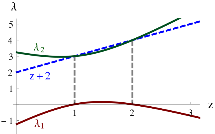
Figure 1: The exponents $\lambda_{1}$ and $\lambda_{2}$ as functions of the dynamical exponent $z$. $\lambda_{1}$ is only positive for $1\leq z\leq 2$, indicating that the corresponding mode becomes non-renormalizable outside this range.

For $1<z<2$ all exponents on the right hand side of (14) are positive, when $z>2$ the exponent $\lambda_{1}$ is negative and the associated mode needs to be tuned to zero because it would otherwise drive the system away from the asymptotically Lifshitz fixed point. A quite comprehensive analysis of the degrees of freedom can be found in [19, 20]. Summarized,

$\bullet\quad\Delta=0$	:	components of a triad describing the geometry in the boundary field theory, these are interpreted as sources for an energy density $\mathpzc{E}$, energy flux $\epsilon^{j}$ and stress tensor $\Pi_{a}^{j}$
$\bullet\quad\Delta=z+2$	:	expectation values for $\mathpzc{E}$, $\epsilon^{j}$ and $\Pi_{a}^{j}$
$\bullet\quad\Delta=2(z-1)$	:	two degrees of freedom, which are interpreted as the source for a vector operator in the boundary field theory – the latter was identified with the momentum $\mathpzc{p}_{a}$ in [19]
$\bullet\quad\Delta=3z$	:	expectation value for $\mathpzc{p}_{a}$
$\bullet\quad\Delta=\lambda_{1}$	:	a single degree of freedom, interpreted as source of a scalar operator $\mathpzc{O}_{P}$ in the boundary field theory – or the expectation value of an operator $\widetilde{\mathpzc{O}}_{P}$ in alternative quantization
$\bullet\quad\Delta=\lambda_{2}$	:	expectation value for $\mathpzc{O}_{P}$ – or source for $\widetilde{\mathpzc{O}}_{P}$ in alternative quantization

What can be noted is that $\bar{b}$ does not source a vector operator in the boundary by itself, but it combines with $\bar{\Sigma}$ to provide sources for independent $\epsilon^{j}$ and $\mathpzc{p}_{a}$. The same can be said about $\bar{a}$ and $\bar{\Omega}$, which combine to source $\mathpzc{E}$ and $\mathpzc{O}_{P}$, respectively $\widetilde{\mathpzc{O}}_{P}$.

Once the degrees of freedom are identified, the question is which fluctuations are stable and which ones would drive the system away from the Lifshitz fixed point. As already mentioned above, there is obviously an instability if $\lambda_{1}<0$ since the backreaction to the geometry would fail to satisfy (11) unless the $\lambda_{1}$-mode is fine-tuned to zero. On the field theory side, this condition means that only alternative quantization is viable and $\langle\widetilde{\mathpzc{O}}_{P}\rangle=0$. A further reduction of the allowed degrees of freedom might come from considering Green’s functions of fluctuations around a Lifshitz background and demanding that all quasinormal frequencies must have negative imaginary part. For $z>2$ such instabilities were found in certain cases [22], but explicit calculation for $z=2$ in the following will reveal that all quasinormal frequencies are in the lower half-plane.

2.2 Stress - Energy Complex

According to the standard dictionary in gauge/gravity duality, a stress-energy tensor for the dual field theory is sourced by the boundary metric. Given that the dual in the case at hand is expected to have Lifshitz scaling symmetry and to be non-relativistic, it seems less convenient to work with a tensor. Instead, a formalism is adopted that uses a tetrad instead of a metric [19, 23]. First, use $\star$ to denote the Hodge star operator on each of the slices with constant $r$ and consider,

$$\star\pi_{P}=\frac{\delta\mathpzc{S}}{\delta P}\;,\quad\star\tau^{A}=\eta_{AB}\frac{\delta\mathpzc{S}}{\delta e^{B}}\;.$$ (16)

The former is simply the dual momentum of $P$, the latter can be seen as the dual momenta of the tetrad $e^{A}$. In [19], the frame $e^{A}$ was chosen such that $P=\xi e^{0}$ for some function $\xi$. That choice conveniently associates the components of $e^{A}$ with the sources of a stress-energy-complex and reduces the remaining degrees of freedom from the vector $P$ to those of a scalar field, as was already indicated in the previous section. This allows to define a stress-energy complex consisting of energy, energy flux, momentum and stress,

$$\mathpzc{E}\longleftrightarrow\tau^{0}(\partial_{t})\;,\quad\epsilon^{j}\longleftrightarrow\tau^{0}\Bigr{|}_{\partial_{t}^{\perp}}\;,\quad\mathpzc{p}_{a}\longleftrightarrow\tau^{a}(\partial_{t})\;,\quad\Pi_{a}^{j}\longleftrightarrow\tau^{a}\Bigr{|}_{\partial_{t}^{\perp}}\;.$$ (17)

These quantities are not completely independent, but subject to some constraints,

$$\langle\dot{\mathpzc{E}}+\mathrm{div}\,\epsilon\rangle = 0\;,$$ (18)

$$\langle\dot{\mathpzc{p}}+\mathrm{div}\,\Pi\rangle = 0\;,$$ (19)

$$\langle z\mathpzc{E}+\mathrm{tr}\,\Pi\rangle = 0\;.$$ (20)

The first two are conservation equations, the last one can be considered as the Lifshitz-equivalent of what in CFT would be having a vanishing trace of the stress-energy tensor. The correspondence (17) may at first sight suggest that it is necessary to choose a specific frame to define a dictionary. This is not really the case. While (17) gives a clear physical interpretation of the actual degrees of freedom of the system, it would be possible to proceed, without major circumstances, to define a dictionary for a generic frame – which seems sensible, given that the latter is only determined by the metric up to an $O(1,3)$ transformation. What however must be kept in mind is a condition that was already implicitly used in the frame in [19]. Namely, in order to ensure to stay on the space of asymptotically Lifshitz solutions it is not allowed to vary all components of $e^{A}$ and $P$ independently. In other words, when choosing a generic parameterization, for example (13), then requiring that the ansatz satisfies (4,5) and (11) simultaneously leads to on-shell conditions that also relate the values of the fields at spatial infinity,

$$\mathfrak{X}\left[\bar{\Omega},\bar{\Sigma},\bar{\Theta},\bar{e}^{i},\bar{a},\bar{b},\bar{c}\right]\Bigr{|}_{r=0}=0\;.$$ (21)

Once the degrees of freedom have been identified, the standard gauge/gravity dictionary can be used when considering derivatives with respect to the degrees of freedom instead of the components of $e^{A}$ and $P$ directly. E.g. with the example (13), $\bar{\Omega}$ can be identified as the source for the energy $\mathpzc{E}$, which can be seen through boosting and rotating the frame $e^{A}$ such that $e^{0}\parallel P$. Then, it is straightforward to calculate the expectation value either in a direct way or by doing a variation under condition (21) and using Leibnitz’s rule,

$$\langle\mathpzc{E}\rangle=\star\frac{\delta\mathpzc{S}}{\delta\bar{\Omega}}=\star\left[\frac{\partial e^{0}}{\partial\bar{\Omega}}\wedge\star\tau^{0}+\frac{\partial e^{1}}{\partial\bar{\Omega}}\wedge\star\tau^{1}+\frac{\partial e^{2}}{\partial\bar{\Omega}}\wedge\star\tau^{2}+\frac{\partial P}{\partial\bar{\Omega}}\wedge\star\pi_{P}\right]\Biggr{|}_{\mathfrak{X}}\;.$$ (22)

2.3 The Case z = 2 and Logarithmic Field Theories

As already could be seen in fig. 1, the case $z=2$ is of particular interest and was thus also subject to some more detailed investigations [12, 24, 25, 26]. At this value, $\lambda_{1}=0$ and the mode associated with it becomes marginal. Furthermore, $\lambda_{2}=4$ and thus the operator $\mathpzc{O}_{P}$ has the same scaling dimension as $\mathpzc{E}$ and $\Pi$. On the gravity side, the general Fefferman–Graham expansion (14) is modified to contain logarithmic terms,

$$\xi=r^{\Delta}\sum\limits_{n\geq 0}\xi^{(n)}r^{2n}+r^{\Delta}\log r\,\sum\limits_{n\geq 0}\widetilde{\xi}^{(n)}r^{2n}+\ldots\;,$$ (23)

where the dots stand for higher powers in logarithms. The degrees of freedom are the same as for $z\neq 2$, only now the ones associated to $\lambda_{1,2}$ have become degrees of freedom in the logarithmic terms at order $0$ and $4$ respectively. Furthermore, having $z+2$ being a multiple of $2$ also results in anomalous terms in the expectation values for the stress-energy complex, i.e. (18-20) can contain non-zero terms on the right hand side,

$$\langle\dot{\mathpzc{E}}+\mathrm{div}\,\epsilon\rangle = \mathpzc{A}_{1}\;,$$ (24)

$$\langle\dot{\mathpzc{p}}+\mathrm{div}\,\Pi\rangle = \mathpzc{A}_{2}\;,$$ (25)

$$\langle 2\mathpzc{E}+\mathrm{tr}\,\Pi\rangle = \mathpzc{A}_{3}\;.$$ (26)

A analysis of the anomalous terms $\mathpzc{A}_{j}$ is a somewhat tedious affair and for further details will therefore be referred to [12, 24, 25, 26]. The remainder of the paper deals with two-point correlation functions at the Lifshitz fixed point in the presence of the aforementioned logarithmic terms. The leading order term was often discarded in an analysis of $z=2$ Lifshitz spacetimes so far, as it fails to satisfy (11). Being logarithmic, it is however a rather mild violation of the asymptotically Lifshitz condition. Such logarithmic deformations have already enjoyed a range of studies in asymptotically AdS spacetimes, like topologically massive gravity (TMG) [27, 28] new massive gravity (NMG) [29] and other higher-derivative gravity theories [30, 31]. They were argued to be duals of a logarithmic conformal field theory (LCFT) [14], which is distinguished from ordinary CFT in that it contains an indecomposable but not diagonalizable highest weight representation. This means that some of the highest weight states form a non-trivial Jordan cell, the size of which is usually called the rank of the indecomposable representation. A comprehensive review of LCFT’s and their features can for example be found in [15, 16, 17]. What will be relevant in the following is that the presence of a Jordan cell will cause the appearance of logarithmic terms in correlation functions. For example, in rank two, assume $\Psi$ is a field of weight $h$ and $\widetilde{\Psi}$ is its (first) logarithmic partner. Then, under some general assumptions about the form of the OPE, two-point correlation functions look as follows,

$$\langle\Psi(z)\Psi(0)\rangle = 0\;,$$ (27)

$$\langle\widetilde{\Psi}(z)\Psi(0)\rangle = \frac{a}{z^{2h}}\;,$$ (28)

$$\langle\widetilde{\Psi}(z)\widetilde{\Psi}(0)\rangle = \frac{-2a\log z+b}{z^{2h}}\;,$$ (29)

for some constants $a,b$ that depend on the normalization of the fields. In the absence of conformal symmetry, the study of field theories with such logarithmic features has not yet enjoyed much attention. First attempts to extend these features to models with Lifshitz scaling symmetry were made [18], but a thorough understanding of these kind of systems is still in its infancy. Nevertheless, a number qualitative results are at hand and by comparing those to the two-point correlation functions that will be calculated in section sec. 5.1, evidence will be unveiled that suggests the massive vector model (1) at the $z=2$ Lifshitz fixed point as a candidate for a gravity dual to a field theory where the energy operator $\mathpzc{E}$ and a scalar operator $\mathpzc{O}_{P}$ combine to form a logarithmic pair.

3 Linearization

A general solution to the system (4,5) is not known, but according to the prescription in [33], it is sufficient to linearize the equations of motion around (8) in order to calculate two-point correlation functions in that background. A perturbation around that fixed point can be parameterized as

$$\delta e^{0} = \frac{\Omega}{2r^{2}}\,\textit{{d}}t+\frac{\Sigma_{1}}{2r^{2}}\,\textit{{d}}x_{1}+\frac{\Sigma_{2}}{2r^{2}}\,\textit{{d}}x^{2}\;,$$ (30)

$$\delta e^{1} = \frac{h_{11}}{2r}\,\textit{{d}}x_{1}+\frac{h_{12}}{2r}\,\textit{{d}}x^{2}\;,$$ (31)

$$\delta e^{2} = \frac{h_{12}}{2r}\,\textit{{d}}x_{1}+\frac{h_{22}}{2r}\,\textit{{d}}x^{2}\;,$$ (32)

$$\delta e^{3} = 0\;,$$ (33)

$$\delta P = \frac{a}{r^{2}}\,\textit{{d}}t+\frac{b_{1}}{r^{2}}\,\textit{{d}}x_{1}+\frac{b_{2}}{r^{2}}\,\textit{{d}}x^{2}+\frac{c}{r}\,\textit{{d}}r\;.$$ (34)

What can also be seen, with regard to the general parameterization (13), is that $\bar{\Theta}^{j}=0$, i.e. there are no timelike components in $e^{j}$. Since $e^{A}$ is only defined up to a $O(1,3)$ transformation, this choice is possible without loss of generality.

3.1 Linearized Equations

Plugging the ansatz (30-34) into the equations of motion (4,5) and going to Fourier space leads to a set of linear ODEs for the perturbations,

$$r^{2}\Omega^{\prime\prime}-4r\Omega^{\prime}+\left(-\frac{k^{2}r^{2}}{2}+6\right)\Omega-\frac{r}{2}h_{11}^{\prime}+\left(\frac{\omega^{2}r^{4}}{2}+\frac{k_{2}^{2}r^{2}}{2}\right)h_{11}\hskip 39.83385pt$$

$$-\frac{r}{2}h_{22}^{\prime}+\left(\frac{\omega^{2}r^{4}}{2}+\frac{k_{1}^{2}r^{2}}{2}\right)h_{22}-k_{1}k_{2}r^{2}h_{12}+3ra^{\prime}-12a\hskip 28.45274pt$$

$$-\frac{\omega k_{1}r^{2}}{2}\Sigma_{1}-\frac{\omega k_{2}r^{2}}{2}\Sigma_{2}+3ir^{2}\omega c = 0\;,$$ (35)

$$r^{2}a^{\prime\prime}-3ra^{\prime}+r^{2}\left(-k_{1}^{2}-k_{2}^{2}\right)a+r\Omega^{\prime}-rh_{11}^{\prime}-rh_{22}^{\prime}\hskip 91.04881pt$$

$$-k_{1}r^{2}\omega b_{1}-k_{2}r^{2}\omega b_{2}+ir^{2}\omega c^{\prime} = 0\;,$$ (36)

$$r^{2}h_{11}^{\prime\prime}-\frac{5}{2}rh_{11}^{\prime}+\left(\frac{\omega^{2}r^{4}}{2}-\frac{k_{2}^{2}r^{2}}{2}\right)h_{11}+\left(\frac{\left(k_{2}^{2}-k_{1}^{2}\right)r^{2}}{2}-2\right)\Omega\hskip 39.83385pt$$

$$-ra^{\prime}+4a+\frac{r}{2}h_{22}^{\prime}+\left(-\frac{\omega^{2}r^{4}}{2}-\frac{k_{1}^{2}r^{2}}{2}\right)h_{22}+k_{1}k_{2}r^{2}h_{12}\hskip 28.45274pt$$

$$-\frac{\omega k_{1}r^{2}}{2}\Sigma_{1}+\frac{\omega k_{2}r^{2}}{2}\Sigma_{2}-ir^{2}\omega c = 0\;,$$ (37)

$$r^{2}h_{22}^{\prime\prime}-\frac{5r}{2}h_{22}^{\prime}+\left(\frac{\omega^{2}r^{4}}{2}-\frac{k_{1}^{2}r^{2}}{2}\right)h_{22}+\left(\frac{\left(k_{1}^{2}-k_{2}^{2}\right)r^{2}}{2}-2\right)\Omega\hskip 39.83385pt$$

$$-ra^{\prime}+4a+\frac{r}{2}h_{11}^{\prime}+\left(-\frac{\omega^{2}r^{4}}{2}-\frac{k_{2}^{2}r^{2}}{2}\right)h_{11}+k_{1}k_{2}r^{2}h_{12}\hskip 28.45274pt$$

$$+\frac{\omega k_{1}r^{2}}{2}\Sigma_{1}-\frac{\omega k_{2}r^{2}}{2}\Sigma_{2}-ir^{2}\omega c = 0\;,$$ (38)

$$r^{2}h_{12}^{\prime\prime}-3rh_{12}^{\prime}+\omega^{2}r^{4}h_{12}-k_{1}k_{2}r^{2}\Omega-\frac{1}{2}k_{2}r^{2}\omega\Sigma_{1}-\frac{1}{2}k_{1}r^{2}\omega\Sigma_{2} = 0\;,$$ (39)

$$r^{2}\Sigma_{1}^{\prime\prime}-5r\Sigma_{1}^{\prime}+\left(-k_{2}^{2}r^{2}+8\right)\Sigma_{1}-2k_{1}r^{4}\omega h_{22}+2k_{2}r^{4}\omega h_{12}+k_{1}k_{2}r^{2}\Sigma_{2}\hskip 45.5244pt$$

$$+4rb_{1}^{\prime}-16b_{1}-4ik_{1}r^{2}c = 0\;,$$ (40)

$$r^{2}\Sigma_{2}^{\prime\prime}-5r\Sigma_{2}^{\prime}+\left(-k_{1}^{2}r^{2}+8\right)\Sigma_{2}-2k_{2}r^{4}\omega h_{11}+2k_{1}r^{4}\omega h_{12}+k_{1}k_{2}r^{2}\Sigma_{1}\hskip 45.5244pt$$

$$+4rb_{2}^{\prime}-16b_{2}-4ik_{2}r^{2}c = 0\;,$$ (41)

$$r^{2}b_{1}^{\prime\prime}-5rb_{1}^{\prime}+\left(\omega^{2}r^{4}-k_{2}^{2}r^{2}+4\right)b_{1}+\omega k_{1}r^{4}a+k_{1}k_{2}r^{2}b_{2}+r\Sigma_{1}^{\prime}-2\Sigma_{1}-ik_{1}r^{3}c^{\prime} = 0\;,$$ (42)

$$r^{2}b_{2}^{\prime\prime}-5rb_{2}^{\prime}+\left(\omega^{2}r^{4}-k_{1}^{2}r^{2}+4\right)b_{2}+\omega k_{2}r^{4}a+k_{1}k_{2}r^{2}b_{1}+r\Sigma_{2}^{\prime}-2\Sigma_{2}-ik_{2}r^{3}c^{\prime} = 0\;,$$ (43)

$$\left(-\omega^{2}r^{4}+k^{2}r^{2}+4\right)c+i\omega r^{2}\Omega+i\omega r^{3}a^{\prime}-2i\omega r^{2}\omega a-i\omega r^{2}h_{11}-i\omega r^{2}\omega h_{22}\hskip 8.53581pt$$

$$+ik_{1}\Sigma_{1}+ik_{2}\Sigma_{2}+ik_{1}rb_{1}^{\prime}-2ik_{1}b_{1}+ik_{2}rb_{2}^{\prime}-2ik_{1}b_{2} = 0\;,$$ (44)

that are subject to some additional constraints,

$$-r\Omega^{\prime}-\frac{k^{2}r^{2}}{2}\Omega-ra^{\prime}-\frac{3r}{2}h_{11}^{\prime}+\left(\frac{\omega^{2}r^{4}}{2}-\frac{k_{2}^{2}r^{2}}{2}\right)h_{11}+k_{1}k_{2}r^{2}h_{12}\hskip 34.14322pt$$

$$-\frac{3r}{2}h_{22}^{\prime}+\left(\frac{\omega^{2}r^{4}}{2}-\frac{k_{1}^{2}r^{2}}{2}\right)h_{22}-\frac{\omega k_{1}r^{2}}{2}\Sigma_{1}-\frac{\omega k_{2}r^{2}}{2}\Sigma_{2}-ir^{2}\omega c = 0\;,$$ (45)

$$-\frac{ik_{1}r}{2}\Omega^{\prime}+\frac{1}{2}ik_{1}\Omega-ik_{1}a+\frac{ik_{2}r}{2}h_{12}^{\prime}-\frac{ik_{1}r}{2}h_{22}^{\prime}-\frac{i\omega r}{4}\Sigma_{1}^{\prime}+\frac{i\omega}{2}\Sigma_{1}^{\prime}-i\omega b_{1} = 0\;,$$ (46)

$$-\frac{ik_{2}r}{2}\Omega^{\prime}+\frac{ik_{2}}{2}\Omega-ik_{2}a-\frac{ik_{2}r}{2}h_{11}^{\prime}+\frac{ik_{1}r}{2}h_{12}^{\prime}-\frac{i\omega r}{4}\Sigma_{2}^{\prime}+\frac{i\omega}{2}\Sigma_{2}^{\prime}-i\omega b_{2} = 0\;,$$ (47)

$$\frac{i\omega r^{3}}{2}h_{11}^{\prime}+\frac{i\omega r^{2}}{2}h_{11}+\frac{i\omega r^{3}}{2}h_{22}^{\prime}+\frac{i\omega r^{2}}{2}h_{22}-\frac{ik_{1}r}{4}\Sigma_{1}^{\prime}-\frac{ik_{2}r}{4}\Sigma_{2}^{\prime}-2c = 0\;.$$ (48)

It should be mentioned that $c$ does not contain any additional degrees of freedom, it is completely determined by the other functions. Nevertheless, introducing $c$ in (34) is crucial, as it would not be possible to solve the equations with all constraints in a meaningful way otherwise. To proceed, it is convenient to split the functions involved into shear and sound modes. For this purpose,

$$h=\left[\begin{array}[]{cc}h_{11}&h_{12}\\ h_{12}&h_{22}\end{array}\right]\;,\quad\mathpzc{J}=\left[\begin{array}[]{cc}&-1\\ 1&\end{array}\right]\;,\quad\Sigma=\left(\begin{array}[]{cc}\Sigma_{1}\\ \Sigma_{2}\end{array}\right)\;,\quad b=\left(\begin{array}[]{cc}b_{1}\\ b_{2}\end{array}\right)\;,\quad k=\left(\begin{array}[]{cc}k_{1}\\ k_{2}\end{array}\right)\;.\quad$$ (49)

Using the shorthand introduced above,

$$\check{h}=\frac{1}{k^{2}}k\cdot h\cdot\mathpzc{J}\cdot k\;,\;\;\check{\Sigma}=k\cdot\mathpzc{J}\cdot\Sigma\;,\;\;\check{b}=k\cdot\mathpzc{J}\cdot b\;,$$ (50)

span the modes of the shear channel that will be analyzed in sec. 4. The sound modes are spanned by

$$\Omega\;,\;\;a\;,\;\;c\;,\;\;\mathrm{tr}\,h\;,\;\;\hat{h}=\frac{1}{k^{2}}k\cdot h\cdot k\;,\;\;\hat{\Sigma}=k\cdot\Sigma\;,\;\;\hat{b}=k\cdot b\;,$$ (51)

and a solution for these modes will be discussed in sec. 5.

3.2 Renormalization and On-Shell Action

In the standard gauge/gravity dictionary, the on-shell gravity action is identified with the generating functional for correlation functions in the dual field theory,

$$\langle O_{1}(x_{1})\cdots O_{n}(x_{n})\rangle = (-i)^{n+1}\frac{\delta^{n}\mathpzc{S}}{\delta J_{1}(x_{1})\cdots\delta J_{n}(x_{n})}\;.$$ (52)

As is often the case, the action functional is not finite for general solutions to the equations of motion and needs to be renormalized,

$$\mathpzc{S}^{ren} = \mathpzc{S}^{bulk}+\mathpzc{S}^{GH}+\mathpzc{S}^{ct}+\mathpzc{S}^{ct,anom}\;,$$ (53)

where $\mathpzc{S}^{GH}$ denotes the usual Gibbosns-Hawking term needed to make the variation of the action well-defined, and the remaining terms on the right hand side are needed to make $\mathpzc{S}^{ren}$ finite on-shell. The term $\mathpzc{S}^{ct,anom}$ denotes anomalous counterterms, i.e. terms needed to cancel logarithmic divergences that arise in the bulk action and are expected to appear for even $z$. These must not be confused with the mechanism behind the appearance of logarithmic terms in the correlation functions, which will be the main topic in sec. 5.1. The former appear due to the dimension of the energy, $z+2$, being a multiple of $2$. Those terms do not introduce new degrees of freedom and are, in fact, completely determined by the curvature and other derivatives of the boundary fields. The logarithmic terms that arise when the exponents of two or more different modes coincide exactly, however, do contain actual degrees of freedom. This is the feature that leads to Jordan cells in the decomposition of the on-shell solution into Eigenstates with respect to the normal Lie derivative $\mathfrak{L}_{n}$. The expectation is that this is related to a similar structure of Jordan cells in representations of the field theory dual.

A systematic procedure to construct $\mathpzc{S}^{ct}$ and $\mathpzc{S}^{ct,anom}$ is holographic renormalization, where an on-shell solution is expanded into a Fefferman–Graham expansion in a radial coordinate $r$ and counterterms are calculated order by order – see e.g. [34, 35] to get an overview. This procedure is in the meanwhile well understood for asymptotically AdS spacetimes. First attempts to extend these results to asymptotically Lifshitz spacetime were presented in [13, 19, 23], more sophisticated descriptions followed [20, 24, 36]. A detailed analysis for the case $z=2$ can be found in [25, 26], where also much attention was devoted to calculating the anomalous terms arising in this case. A maybe somewhat more convenient and elegant way for a holographic renormalization of a $z=2$ Lifshitz spacetime was presented in [12], via an embedding into an asymptotically AdS spacetime where holographic renormalization is well understood. This procedure also included the leading logarithmic divergence that was discarded in most of the previously mentioned publications.

For the purpose of this paper, however, using the full formalism for holographic renormalization and calculating anomalous terms seems a bit like breaking a butterfly upon a wheel. As already mentioned before, two-point functions can be calculated via a linearization of the equations of motion. This means that in order to obtain all necessary information it is sufficient to know the action up to quadratic order. Counterterms that render the action finite at this level of detail can be constructed in a rather straightforward way – an explicit expression can be found in app. A. There is a certain ambiguity in these counterterms, as they are only determined up to finite contributions by the requirement to cancel divergences of the action on-shell. Knowing these contributions would be crucial in order to calculate anomalous terms in one-point functions, but for two-point functions they would only contribute as contact terms and will thus be of little significance in the following.

Renormalization results in an explicit expression for the on-shell action at quadratic order. As mentioned above, an asymptotic expansion for a general solution of (35-48) can perturbatively be found by making a generalized power series ansatz like (23) and demanding that this series solves the equations of motion. This will result in various conditions relating the coefficients, which can be calculated order by order. To find an explicit expression for the on-shell action at the boundary at quadratic order it is sufficient to calculate these coefficients up to order $6$ and then inserting the series into (53). After a somewhat tedious calculation, the on-shell action can be expressed as,

$$\mathpzc{S}^{on-shell} = \frac{1}{2\kappa}\frac{1}{(2\pi)^{3}}\int\langle X,\mathpzc{M}X\rangle\,\textit{{d}}\omega\,\textit{{d}}^{2}k+\mathpzc{O}(x_{3},(\omega+k^{2})^{2})\;.$$ (54)

The last term on the right hand side is there to remind that the on-shell action is determined up to quadratic order and derivative corrections that would only contribute as contact terms in two-point functions and will thus not be considered in the following. Using the notation (49), expressions for $X$ and $\mathpzc{M}$ can be given,

$$X = \left(\Omega^{(0)},\,\widetilde{\Omega}^{(0)},\,\check{\Sigma}^{(2)},\,\hat{\Sigma}^{(2)},\,\check{\Sigma}^{(0)},\,\hat{\Sigma}^{(0)},\,\mathrm{tr}\,h^{(0)},\,\hat{h}^{(0)},\,\check{h}^{(0)},\,\check{\mathpzc{u}},\,\hat{\mathpzc{v}},\,\check{\mathpzc{v}},\,T,\,\widetilde{T}\right)\;,$$ (55)

$$\mathpzc{M} = \frac{1}{2}\left[\begin{array}[]{cccccccccccccc}&&&&&&&&&&&&&1\\ &&&&&&&&&&&&1&\\ &&&&&&&&&&&1&&\\ &&&&&&&&&&1&&&\\ &&&&&&&&&1&&&&\\ &&&&&&&&&&&&&\frac{\omega}{k^{2}}\\ &&&&&&&&&&\omega&&&-2\\ &&&&&&&&&&-2\omega&&&2\\ &&&&&&&&&&&2\omega&&\\ &&&&1&&&&&&&&&\\ &&&1&&&\omega&-2\omega&&&&&&\\ &&1&&&&&&2\omega&&&&&\\ &1&&&&&&&&&&&&\\ 1&&&&&\frac{\omega}{k^{2}}&-2&2&&&&&&\end{array}\right]\;.$$ (70)

In (55), the index $(2j)$ refers to the order of the coefficient in the generalized power series (23), the last five terms are,

$$\widetilde{T}=-\widetilde{\Omega}^{(4)}\;,\quad T=2\Omega^{(4)}-\frac{5}{2}\widetilde{\Omega}^{(4)}\;,\quad\hat{\mathpzc{v}}=\frac{1}{2k^{2}}\hat{\Sigma}^{(4)}\quad\check{\mathpzc{v}}=\frac{1}{2k^{2}}\check{\Sigma}^{(4)}\;\quad\check{\mathpzc{u}}=\frac{3}{2k^{2}}\check{\Sigma}^{(6)}\;.$$ (71)

As explained in sec. 2.1, the modes $\Omega^{(0)}$, $h^{(0)}$, $\Sigma^{(0)}$ and $\Sigma^{(2)}$ can be associated with the sources for the energy $\mathpzc{E}$, stress $\Pi$, energy flux $\epsilon$ and momentum $\mathpzc{p}$. In accordance with (24-26) follows,

$$\langle\dot{\mathpzc{E}}+\mathrm{div}\,\epsilon\rangle = \mathpzc{O}((\omega+k^{2})^{2})\;,$$ (72)

$$\langle\dot{\mathpzc{p}}+\mathrm{div}\,\Pi\rangle = \mathpzc{O}((\omega+k^{2})^{2})\;,$$ (73)

$$\langle 2\mathpzc{E}+\mathrm{tr}\,\Pi\rangle = \mathpzc{O}((\omega+k^{2})^{2})\;.$$ (74)

Again, the term on the right hand side is there to remind that derivative correction are expected, but they will not be of importance for the following calculations. Despite the few shortcomings in the calculation of expectation values, the quadratic on-shell action (54) contains all necessary information to extract the data for two-point functions. These correspond to the Green’s functions of the fields in the linearized equations (35-48). Examining these in the next sections will also allow to shed some light on the role of the scalar operator sourced by $\widetilde{\Omega}^{(0)}$, which has the same dimension as $\mathpzc{E}$ and $\Pi$.

4 Shear Channel

The shear modes (50) can be combined into two master fields,

$$\mathpzc{X}=\check{h}+\frac{1}{2\omega r^{2}}\left(\check{\Sigma}-2\check{b}\right)\;,\quad\mathpzc{Y}=\frac{1}{\omega^{2}r^{3}}\left(\check{\Sigma}^{\prime}-2\check{b}^{\prime}\right)-\frac{2}{\omega^{2}r^{4}}\left(\check{\Sigma}^{\prime}-2\check{b}^{\prime}\right)\;.$$ (75)

These solve a set of decoupled second order differential equations,

$$v^{2}\mathpzc{X}^{\prime\prime}-v\mathpzc{X}^{\prime}+v\left(2v-\lambda\right)\mathpzc{X} = 0\;,$$ (76)

$$v^{2}\mathpzc{Y}^{\prime\prime}+v\left(v-\frac{\lambda}{2}\right)\mathpzc{Y} = 0\;,$$ (77)

which used the substitution of variables,

$$v=\frac{r^{2}}{2\omega}\;,\quad\lambda=\frac{k^{2}}{\omega}\;.$$ (78)

A general analytic solution to (76,77) can be written as follows,

$$\mathpzc{X} = A{X}e^{iv}\,\Gamma\left(1+\frac{i\lambda}{4}\right)U\left(\frac{i\lambda}{4},0,-2iv\right)+B{X}e^{-iv}\,\Gamma\left(1-\frac{i\lambda}{4}\right)U\left(-\frac{i\lambda}{4},0,2iv\right)\;,$$ (79)

$$\mathpzc{Y} = A{Y}e^{iv}\,v^{2}\,\Gamma\left(\frac{6+i\lambda}{4}\right)U\left(\frac{6+i\lambda}{4},3,-2iv\right)+B{Y}e^{-iv}\,v^{2}\,\Gamma\left(\frac{6-i\lambda}{4}\right)U\left(\frac{6-i\lambda}{4},1,2iv\right)\;.\qquad$$ (80)

In these expressions, $U$ stands for the Tricomi function which is a solution to the confluent hypergeometric differential equation. This function has a branch cut in the third argument along the negative real axis. Explicit expressions for the shear modes follow immediately,

$$\check{h} = \mathpzc{X}+\frac{1}{2}\int\mathpzc{Y}\;,$$ (81)

$$\check{\Sigma} = -2\lambda\mathpzc{X}+2\mathpzc{Y}-2v\mathpzc{Y}^{\prime}-2v\int\mathpzc{Y}\;,$$ (82)

$$\check{b} = -\lambda\mathpzc{X}+\mathpzc{Y}-v\mathpzc{Y}^{\prime}\;.$$ (83)

As the intent is to calculate retarded Green’s functions, (79,80) will be subject to infalling wave condition in the interior, which means $A_{\mathpzc{X},\mathpzc{Y}}=0$. Demanding (12) to be satisfied would furthermore induce a relation between $B_{\mathpzc{X}}$ and $B_{\mathpzc{Y}}$. However, in order to calculate correlation functions, this condition will not be imposed on-shell in the following. Keeping in mind that there is an integration constant in (81-83), this leaves three degrees of freedom. These could be parameterized by $\check{h}^{(0)}$, $\check{\Sigma}^{(0)}$ and $\check{\Sigma}^{(2)}$, other modes in the shear channel can then be expressed via those coefficients,

$$\check{\mathpzc{v}} = \frac{\omega\left[\psi_{1}+4\ln\left(-i\omega\right)\right]}{32}\,\check{h}^{(0)}+\frac{\omega\left[\lambda^{2}-4+\lambda\psi_{2}\right]}{64\lambda}\,\check{\Sigma}^{(0)}+\frac{\psi_{1}+4\ln\left(-i\omega\right)}{64}\,\check{\Sigma}^{(2)}\;,$$ (84)

$$\check{\mathpzc{u}} = \frac{\omega^{2}\psi_{2}}{32}\,\check{h}^{(0)}+\frac{\omega^{2}\left\{24\left(\lambda^{2}+2\right)\psi_{2}-\lambda\left(\lambda^{2}+4\right)\left[3\psi_{1}-28+12\ln\left(-i\omega\right)\right]\right\}}{3072\lambda}\,\check{\Sigma}^{(0)}+\frac{\omega\psi_{2}}{64}\,\check{\Sigma}^{(2)}\;.\;$$ (85)

The $\psi_{j}$ are substitutions for expressions that involve the Euler–Mascheroni constant $\gamma$ and the digamma function $\psi$,

$$\psi_{1} = 2i\lambda-6+8\gamma-\lambda^{2}\psi\left(\frac{i\lambda}{4}\right)+\left(\lambda^{2}+4\right)\psi\left(\frac{i\lambda+2}{4}\right)\;,$$ (86)

$$\psi_{2} = \frac{1}{4}\left[2i\lambda^{2}-4\lambda^{2}+8i-\lambda\left(\lambda^{2}+4\right)\psi\left(\frac{i\lambda}{4}\right)+\lambda\left(\lambda^{2}+4\right)\psi\left(\frac{i\lambda+2}{4}\right)\right]\;.$$ (87)

Following the standard prescription [33] it is now straightforward to obtain the retarded Green’s functions, respectively two-point correlation functions, for the operators in the shear channel from these expressions. These operators are the transversal components of the stress $\check{\Pi}$, the momentum $\check{\mathpzc{p}}$ and the energy flux $\check{\epsilon}$. The identity (72) induces certain relations between various correlators,

$$\langle\check{\mathpzc{p}}\,\check{\mathpzc{p}}\rangle=\lambda\langle\check{\Pi}\,\check{\mathpzc{p}}\rangle=\lambda^{2}\langle\check{\Pi}\,\check{\Pi}\rangle\;,\quad\langle\check{\mathpzc{p}}\,\check{\epsilon}\rangle=\lambda\langle\check{\Pi}\,\check{\epsilon}\rangle\;,$$ (88)

leaving three independent two-point correlation functions. These can be expressed via derivatives of (84,85) with respect to the sources $\check{h}^{(0)}$, $\check{\Sigma}^{(0)}$ and $\check{\Sigma}^{(2)}$. Up to contact terms,

$$\langle\check{\mathpzc{p}}\,\check{\mathpzc{p}}\rangle = \frac{i\omega^{2}\lambda^{2}}{32(2\pi)^{3}\kappa}\left[\psi_{1}+4\ln\left(-i\omega\right)\right]\;,$$ (89)

$$\langle\check{\mathpzc{p}}\,\check{\epsilon}\rangle = -\frac{i\omega^{3}\lambda^{2}\psi_{2}}{32(2\pi)^{3}\kappa}\;,$$ (90)

$$\langle\check{\epsilon}\,\check{\epsilon}\rangle = -\frac{i\omega^{4}\lambda}{512(2\pi)^{3}\kappa}\left[\lambda(\lambda^{2}+4)\psi_{1}-8(\lambda^{2}+2)\psi_{2}+4\lambda(\lambda^{2}+4)\ln\left(-i\omega\right)\right]\;.$$ (91)

These correlators can only have poles where $\psi_{1,2}$ have, that is for $\lambda=2in$, $n\geq 2$. This implies that all quasinormal frequencies of the shear channel are on the negative imaginary half-axis and fluctuations in these modes do not cause instabilities.

5 Sound Channel

To construct a general solution for the sound modes (51), it is convenient to introduce the master field $\mathpzc{Z}=\Omega-2a$, which can be shown to satisfy a sixth order differential equation,

$$\mathfrak{D}^{3}\frac{1}{v}\mathfrak{D}^{2}\frac{1}{v^{2}}\mathfrak{D}^{1}\mathpzc{Z} = 0\;,$$ (92)

which used the substitutions (78). The $\mathfrak{D}^{j}$ denote second order differential operators,

$$\mathfrak{D}^{1} = v^{2}\partial_{v}^{2}+v\left(v-\frac{\lambda}{2}\right)\;,$$ (93)

$$\mathfrak{D}^{2} = v^{2}\partial_{v}^{2}+v\partial_{v}+v\left(v+2i-\frac{\lambda}{2}\right)\;,$$ (94)

$$\mathfrak{D}^{3} = v^{2}\partial_{v}^{2}+v\partial_{v}+v\left(v-2i-\frac{\lambda}{2}\right)\;.$$ (95)

A general analytic solution for (92) can be found by introducing functions $\Upsilon^{j}$ which parameterize the kernels of the operators (93-95), i.e. $\mathfrak{D}^{j}\Upsilon^{j}=0$. Explicitly,

$$\Upsilon^{1} = A_{1}e^{iv}\,\Gamma\left(1+\frac{i\lambda}{4}\right)U\left(\frac{i\lambda}{4},0,-2iv\right)+B_{1}e^{-iv}\,\Gamma\left(1-\frac{i\lambda}{4}\right)U\left(-\frac{i\lambda}{4},0,2iv\right)\;,\quad$$ (96)

$$\Upsilon^{2} = A_{2}e^{iv}\,\Gamma\left(\frac{6+i\lambda}{4}\right)U\left(\frac{6+i\lambda}{4},1,-2iv\right)+B_{2}e^{-iv}\,\Gamma\left(\frac{-2-i\lambda}{4}\right)U\left(\frac{-2-i\lambda}{4},1,2iv\right)\;,\quad$$ (97)

$$\Upsilon^{3} = A_{3}e^{iv}\,\Gamma\left(\frac{-2+i\lambda}{4}\right)U\left(\frac{-2+i\lambda}{4},1,-2iv\right)+B_{3}e^{-iv}\,\Gamma\left(\frac{6-i\lambda}{4}\right)U\left(\frac{6-i\lambda}{4},1,2iv\right)\;.\quad$$ (98)

Again, imposing that viable solutions must satisfy ingoing boundary conditions in the interior implies $A_{j}=0$. By means of (96-98) a solution for $\mathpzc{Z}$ can then be constructed explicitly and from there it is straightforward to successively find expressions for the other functions in the sound channel. Summarized, they are all of the form,

$$q_{0}(v)+q_{1}(v)\Upsilon^{j}(v)+q_{2}(v){\Upsilon^{j}}^{\prime}(v)+q_{3}(v)\mathpzc{I}^{j}(v)\;,$$ (99)

with

$$\mathpzc{I}^{j}(v) = \int_{v}^{\infty}\left[p_{1}(w)\Upsilon^{j}(w)+p_{2}(w){\Upsilon^{j}}^{\prime}(w)\right]\textit{{d}}w\;,$$ (100)

and polynomial expressions $q_{j}$ and $p_{j}$. For explicit formulæ is referred to app. B. From these results follows a parameterization for the boundary values of the bulk fields,

$$\Omega^{(0)}=\left[\psi_{3}+\lambda\ln\left(-i\omega\right)\right]\upsilon_{1}+\left[\psi_{4}+(\lambda^{2}+4)\ln\left(-i\omega\right)\right]\upsilon_{2}+2\lambda^{2}\upsilon_{3}-2(\lambda^{2}-4)\upsilon_{4}-8\upsilon_{5}-\upsilon_{6}\;,$$

$$\widetilde{\Omega}^{(0)}=\lambda\upsilon_{1}+(\lambda^{2}+4)\upsilon_{2}\;,\quad\mathrm{tr}\,h^{(0)}=(\lambda^{2}+4)\upsilon_{3}\;,\quad\hat{h}^{(0)}=(\lambda^{2}+4)\upsilon_{4}\;,$$

$$\hat{\Sigma}^{(2)}=\omega(\lambda^{2}+4)\upsilon_{5}\;,\quad\hat{\Sigma}^{(0)}=\lambda\upsilon_{6}\;,$$ (101)

and their conjugate momenta,

$$T = \frac{\omega^{2}\left[3\lambda(\lambda^{2}+4)-\lambda^{2}\psi_{3}-\lambda^{3}\ln\left(-i\omega\right)\right]}{64}\upsilon_{1}$$ (102)

$$\qquad+\frac{\omega^{2}\left[3(\lambda^{2}+4)^{2}-(\lambda^{2}-4)\psi_{4}-(\lambda^{4}-16)\ln\left(-i\omega\right)\right]}{64}\upsilon_{2}$$

$$\qquad+\frac{\omega^{2}(\lambda^{2}+2)}{2}\upsilon_{3}-\frac{\omega^{2}\lambda^{2}}{2}\upsilon_{4}-\omega^{2}\upsilon_{5}\;,$$

$$\widetilde{T} = \frac{\omega^{2}\lambda\left(\lambda^{2}+8\right)}{64}\upsilon_{1}+\frac{\omega^{2}\left(\lambda^{2}+4\right)^{2}}{64}\upsilon_{2}\;,$$ (103)

$$\hat{\mathpzc{v}} = \frac{\omega\left(\lambda^{2}+4\right)\left[7\lambda-4\psi_{3}-4\lambda\ln\left(-2i\omega\right)\right]}{64}\upsilon_{1}+\frac{\omega\left[7\lambda^{2}-4-4\psi_{4}-4(\lambda^{2}+4)\lambda\ln\left(-i\omega\right)\right]}{64}\upsilon_{2}$$ (104)

$$\qquad+\frac{\omega\left[-2(3\lambda^{2}+8)+\psi_{4}+(\lambda^{2}+4)\ln\left(-i\omega\right)\right]}{16}\upsilon_{3}$$

$$\qquad-\frac{\omega\left[(3\lambda^{2}+4)-\psi_{4}-(\lambda^{2}+4)\ln\left(-i\omega\right)\right]}{8}\upsilon_{4}+\frac{\omega\left[8+\psi_{4}+(\lambda^{2}+4)\ln\left(-i\omega\right)\right]}{16}\upsilon_{5}\;.$$

The $\upsilon_{j}$ are just auxiliary variables to parameterize degrees of freedom, and, again, the $\psi_{j}$ stand for expressions that involve the Euler–Mascheroni constant and the digamma function,

$$\psi_{3} = \frac{1}{2}\left[-3\lambda+4\gamma\lambda-4i+\lambda\psi\left(\frac{i\lambda}{4}\right)\right]\;,$$ (105)

$$\psi_{4} = \frac{1}{2}\left[-3\lambda^{2}+4+4\gamma(\lambda^{2}+4)+(\lambda^{2}+4)\psi\left(\frac{i\lambda+2}{4}\right)\right]\;.$$ (106)

The operators sourced by (101) are the energy $\mathpzc{E}$, an other scalar operator $\widetilde{\mathpzc{E}}$ that will be identified as the logarithmic partner of the energy, as well as the longitudinal components of the stress $\hat{\Pi}$, the momentum $\hat{\mathpzc{p}}$ and the energy flux $\hat{\epsilon}$. Due to the conservation equation (25) and the trace condition (26) the correlators of these operators satisfy a series of identities,

$$\langle\mathpzc{E}\,\mathpzc{E}\rangle = -\frac{1}{2}\langle\mathpzc{E}\,\mathrm{tr}\Pi\ \rangle=\frac{1}{\omega}\langle\hat{\epsilon}\,\mathpzc{E}\rangle=\frac{1}{4}\langle\mathrm{tr}\Pi\,\mathrm{tr}\Pi\rangle=-\frac{1}{2\omega}\langle\hat{\epsilon}\,\mathrm{tr}\Pi\rangle=\frac{1}{\omega^{2}}\langle\hat{\epsilon}\,\hat{\epsilon}\rangle\;,$$ (107)

$$\langle\widetilde{\mathpzc{E}}\,\mathpzc{E}\rangle = -\frac{1}{2}\langle\widetilde{\mathpzc{E}}\,\mathrm{tr}\Pi\rangle=\frac{1}{\omega}\langle\widetilde{\mathpzc{E}}\,\hat{\epsilon}\rangle\;,$$ (108)

$$\langle\hat{\mathpzc{p}}\,\mathpzc{E}\rangle = -\frac{1}{2}\langle\hat{\mathpzc{p}}\,\mathrm{tr}\Pi\rangle=\frac{1}{\omega}\langle\hat{\mathpzc{p}}\,\hat{\epsilon}\rangle=\lambda\langle\hat{\Pi}\,\mathpzc{E}\rangle=-\frac{\lambda}{2}\langle\hat{\Pi}\,\mathrm{tr}\Pi\rangle=\frac{\lambda}{\omega}\langle\hat{\Pi}\,\hat{\epsilon}\rangle\;,$$ (109)

$$\langle\hat{\mathpzc{p}}\,\widetilde{\mathpzc{E}}\rangle = \lambda\langle\hat{\Pi}\,\widetilde{\mathpzc{E}}\rangle\;,$$ (110)

$$\langle\hat{\mathpzc{p}}\,\hat{\mathpzc{p}}\rangle = \lambda\langle\hat{\Pi}\,\hat{\mathpzc{p}}\rangle=\lambda^{2}\langle\hat{\Pi}\,\hat{\Pi}\rangle\;.$$ (111)

This leaves six independent two-point functions. Extracting these from the on-shell solution is a bit more involved than it was in the shear channel, but despite a little bit of algebra to invert (101) it is again rather straightforward,

$$\langle\mathpzc{E}\,\mathpzc{E}\rangle = -\frac{i\omega^{2}\lambda(\lambda^{2}+4)}{8\kappa(2\pi)^{3}\Phi}\;,$$ (112)

$$\langle\widetilde{\mathpzc{E}}\mathpzc{E}\rangle = \frac{i\omega^{2}\lambda(\lambda^{2}+4)}{8\kappa(2\pi)^{3}\Phi}\ln\left(-i\omega\right)+\frac{i\omega^{2}\left[(\lambda^{2}+4)\psi_{3}+\lambda\psi_{4}\right]}{16\kappa(2\pi)^{3}\Phi}\;,$$ (113)

$$\langle\widetilde{\mathpzc{E}}\widetilde{\mathpzc{E}}\rangle = -\frac{i\omega^{2}\lambda(\lambda^{2}+4)}{8\kappa(2\pi)^{3}\Phi}\ln\left(-i\omega\right)^{2}-\frac{i\omega^{2}\left[(\lambda^{2}+4)\psi_{3}+\lambda\psi_{4}\right]}{8\kappa(2\pi)^{3}\Phi}\ln\left(-i\omega\right)-\frac{i\omega^{2}\psi_{3}\psi_{4}}{8\kappa(2\pi)^{3}\Phi}\;,$$ (114)

$$\langle\hat{\mathpzc{p}}\,\mathpzc{E}\rangle = \frac{i\omega^{2}\lambda^{2}}{\kappa(2\pi)^{3}\Phi}\;,$$ (115)

$$\langle\hat{\mathpzc{p}}\,\widetilde{\mathpzc{E}}\rangle = -\frac{2i\omega^{2}\lambda\left[\psi_{3}+\lambda\ln\left(-i\omega\right)\right]}{\kappa(2\pi)^{3}\Phi}\;,$$ (116)

$$\langle\hat{\mathpzc{p}}\,\hat{\mathpzc{p}}\rangle = -\frac{i\omega^{2}\lambda^{2}}{8\kappa(2\pi)^{3}(\lambda^{2}+4)}\left[\frac{64\lambda}{\Phi}-\psi_{4}-(\lambda^{2}+4)\ln\left(-i\omega\right)\right]\;.$$ (117)

The function $\Phi$ appearing in the denominator of the expressions above is related to the determinant of the set of linear equations (101) and can be expressed in closed form,

$$\Phi = 2i\lambda^{2}+8\lambda+8i-\left(\lambda^{2}+4\right)\lambda\psi\left(\frac{i\lambda}{4}\right)+\left(\lambda^{2}+4\right)\lambda\psi\left(\frac{i\lambda+2}{4}\right)\;.$$ (118)

Though it may not appear so at first sight, the correlator in (117) is actually regular at $\lambda=-2i$. It easily can be verified that the residue at that point vanishes due to $\psi_{4}(-2i)=8$ and $\Phi(-2i)=-16i$. Furthermore, $\Phi$ cancels the poles coming from the numerator. Thus, with the exception of $\langle\hat{\mathpzc{p}}\,\hat{\mathpzc{p}}\rangle$ that also contains poles at $\lambda=2(2n+1)i$, $n\geq 1$, all quasinormal modes are determined by the zeros of (118). A closed expression for those values is not at hand, but it is possible to argue stability in the sound channel by showing that these zeros must all be located in the upper half of the complex $\lambda$-plane. For this purpose, define,

$$\xi(\mu,\nu)=\Re\Phi(\mu+i\nu)\;,\quad\eta(\mu,\nu)=\Im\Phi(\mu+i\nu)\;.$$ (119)

The zeros of $\Phi$ then correspond to the intersections of the set of curves defined by $\xi=0$ and $\eta=0$. The non-existence of zeros in the lower half-plane follows if it can be shown that $\eta$ is nowhere zeros in that region. This will be done by excluding all other possibilities. As $\eta$ is a harmonic function that asymptotes to $6\nu\left(1+\frac{2}{\mu^{2}+\nu^{2}}\right)$ for large $|\mu|$ and $|\nu|$, the set $\eta=0$ in the lower half-plane must be a collection of smooth curves, each of which must be in one of three possible categories,

1. a bounded closed curve in ${\mathbb{R}}_{<0}\times{\mathbb{R}}$,

2. a bounded curve that intersects with the real axis $\nu=0$,

3. a curve that asymptotes to the real axis $\nu=0$ for large $|\nu|$.

Case (i) would imply that the curve would encircle a pole. This is impossible as all poles of $\Phi$ are in the upper half-plane. Case (ii) can be excluded by examining $\eta$ on the real axis,

$$\eta(\mu,0)=-\frac{\pi\mu\,(4+\mu^{2})}{\mathrm{Sinh}\left(\frac{\pi\mu}{2}\right)}\;,$$ (120)

which is strictly negative. Finally, to exclude case (iii), consider

$$\frac{\partial\eta(\mu,0)}{\partial\nu} \;\;\stackrel{{\scriptstyle\mu\to\pm\infty}}{{\xrightarrow{\hskip 31.29802pt}}}\;\; 6+\frac{12}{\mu^{2}}\;.$$ (121)

Together with $\eta(\mu,0)$ being strictly negative on the real axis, this implies that the curve that asymptotes to the real axis must lie in the upper half-plane. This finishes the proof that $\Phi$ has no zeros with negative imaginary part.

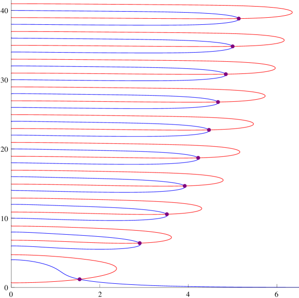
Figure 2: The zeros of $\Phi$ in the right upper half-plane. Red curves mark the vanishing of the real part, blue curves the vanishing of the imaginary part. The intersections, marked by the purple dots, are the zeros.

Analyzing the positions of zeros in the upper half-plane is more complicated. What can be shown in a straightforward way is that there can be no zeros on the imaginary axis. The condition $\Phi(0,\nu)=0$ is equivalent to finding real solutions of

$$\frac{2\pi\nu\,(\nu-2)}{\sin\left(\frac{\pi\nu}{2}\right)} = \nu\,(\nu-2)\left[\psi\left(\frac{\nu+2}{4}\right)-\psi\left(\frac{\nu+4}{4}\right)\right]+\frac{2\,(\nu^{2}-4\nu-4)}{(\nu+2)}\;.$$ (122)

For positive $\nu$, the right hand side is a negative function bounded from below by $-6$, whereas the minimum of the absolute value of the left hand side in this range is $2\pi$. Hence, (122) can have no real solutions. There are however zeros of $\Phi$ away from the imaginary axis. In a similar fashion as before, it is possible to analyze what restrictions the poles and extrema on the imaginary axis impose on the curves $\xi=0$ and $\eta=0$. The conclusion is that there must be an infinite set of intersections of these curves away from the imaginary axis and the zeros of $\Phi$ therefore consist of an infinite set of pairs $\{\lambda,-\bar{\lambda}\}$. For large $n\in{\mathbb{N}}$, there must be one such pair with $4n>\Im\lambda>4n-2$, but finding exact values for zeros was beyond the scope of analytic methods and it was necessary to resort to numerics, a plot is shown in fig. 2.

5.1 Logarithmic structure in two-point correlation functions

This section deals with $\mathpzc{E}$ and $\widetilde{\mathpzc{E}}$, i.e. the operators sourced by $\Omega^{(0)}$ and $\widetilde{\Omega}^{(0)}$ respectively. The aim is to identify $\widetilde{\mathpzc{E}}$ as a logarithmic partner of the energy operator $\mathpzc{E}$ by comparing their two-point functions to (27-29), that is to the structure of increasing powers of logarithmic terms appearing when operators belong to an indecomposable non-diagonalizable representation. The correlators (112-114) are already quite suggestive about the existence of such a tower of logarithmic terms, though in order to have a more elementary comparison it would be desirable to have an expression in position space. Unfortunately, given the complicated form of the denominator, translating the momentum space correlators back to position space in all generality seems out of question. Though, due to a general knowledge of the position of poles and other features of the functions, it is still possible to qualitatively deduce the underlying structure of two-point correlation functions,

$$\langle\mathpzc{E}(t,x)\,\mathpzc{E}(0,0)\rangle = \frac{\theta(t)}{t^{4}}\,\mathpzc{g}^{(0)}(\chi)\;,$$ (123)

$$\langle\widetilde{\mathpzc{E}}(t,x)\,\mathpzc{E}(0,0)\rangle = \frac{\theta(t)\ln t}{t^{4}}\,\mathpzc{g}^{(0)}(\chi)+\frac{\theta(t)}{t^{4}}\,\mathpzc{g}^{(1)}(\chi)\;,$$ (124)

$$\langle\widetilde{\mathpzc{E}}(t,x)\,\widetilde{\mathpzc{E}}(0,0)\rangle = \frac{\theta(t)\ln^{2}t}{t^{4}}\,\mathpzc{g}^{(0)}(\chi)+\frac{\theta(t)\ln t}{t^{4}}\,\mathpzc{g}^{(2)}(\chi)+\frac{\theta(t)}{t^{4}}\,\mathpzc{g}^{(3)}(\chi)\;.$$ (125)

The functions $\mathpzc{g}^{(j)}$ solely depend on the ratio $\chi=x^{2}/4t$, as is to be expected for a theory with $z=2$ Lifshitz scaling. Further details about the transformation back to position space can be found in app. C. The structure of these two-point functions bears a resemblance to the logarithmic field theory with Lifshitz scaling developed in [18]. The power in the prefactor suggests that $\mathpzc{E}$ and $\widetilde{\mathpzc{E}}$ are operators with dimension $2$ with respect to $t$, respectively $4$ with respect to $x$, consistent with the interpretation of energy in a theory with Lifshitz scaling. The mechanism behind the appearance of this logarithmic pair can be argued as follows. For general dynamical exponent $z$ a Lifshitz fixed point can occur when there is a certain relation between the timelike component of the tetrad $e^{0}$ and the Proca field $P$. The modes of these two fields combine to form sources for a set of operators in the dual field theory – in particular $\mathpzc{E}$ and $\mathpzc{O}_{P}$ – which, generically, would be part of a diagonalizable representation of the underlying algebra. The limit $z\to 2$ induces a degeneracy that requires to introduce Jordan cells to get a complete description and, taking CFT as a guideline, it is exactly the appearance of such cells that would make the field theory logarithmic.

The most striking difference is the presence of $\mathpzc{g}^{(0)}$, i.e. that when comparing to the LCFT correlators (27-29) one would expect $\mathpzc{g}^{(0)}=0$. This term did also not appear in the toy model in [18]. However, the vanishing of the right hand side of (27) is only stringent for a LCFT with proper primaries and it thus could have a non-zero value if the OPE of two primaries contains logarithmic fields. Beyond that, other conditions that require the vanishing of this two-point function are related to the underlying conformal symmetry. Therefore it stands to reason that requiring a less stringent level of symmetry – like anisotropic scaling – would also be less restrictive about the values of certain coefficients in the correlation functions.

The function $\mathpzc{g}^{(0)}$ also distinguishes itself from $\mathpzc{g}^{(1,2,3)}$ in that it for $t\ll x^{2}$, respectively $\chi\gg 1$, incorporates a certain ultralocal and oscillatory behavior,

$$\mathpzc{g}^{(0)} \propto \chi^{3}e^{-\Im\lambda_{\min}\chi}\Re\left[\mathpzc{A}\,L_{3}\left(-i\lambda_{\min}\chi\right)e^{i\Re\lambda_{\min}\chi}\right]\;,$$ (126)

where $\mathpzc{A}$ is an amplitude that depends on $\lambda_{\min}$, the latter being a zero of $\Phi$ with minimal imaginary part. The other functions are only expected to follow a power law in this limit, such that for fixed $t>0$ and $x^{2}\gg t$,

$$\langle\mathpzc{E}(t,x)\,\mathpzc{E}(0,0)\rangle \stackrel{{\scriptstyle x^{2}\gg t}}{{\xrightarrow{\hskip 22.76219pt}}} 0\;,$$ (127)

$$\langle\widetilde{\mathpzc{E}}(t,x)\,\mathpzc{E}(0,0)\rangle \stackrel{{\scriptstyle x^{2}\gg t}}{{\xrightarrow{\hskip 22.76219pt}}} \frac{A^{(1)}}{x_{4}}\;,$$ (128)

$$\langle\widetilde{\mathpzc{E}}(t,x)\,\widetilde{\mathpzc{E}}(0,0)\rangle \stackrel{{\scriptstyle x^{2}\gg t}}{{\xrightarrow{\hskip 22.76219pt}}} \frac{A^{(2)}\ln x}{x_{4}}+\frac{A^{(3)}}{x_{4}}\;,$$ (129)

with some constants $A^{(j)}$. Interestingly, up to normalization, this agrees well with (27-29), i.e. the expected form of two-point functions in a LCFT and can be seen as a further indication that the underlying structure in the correlators (123-125) is indeed an extension of the concept of logarithmic field theories to the case of anisotropic scaling symmetry. In the opposite limit, i.e. fixed $x$ and $t\gg x^{2}$, the functions $\mathpzc{g}^{(j)}$ can be expanded in a power series. Including terms up to first order,

$$\langle\mathpzc{E}(t,x)\,\mathpzc{E}(0,0)\rangle \stackrel{{\scriptstyle t\gg x^{2}}}{{\xrightarrow{\hskip 22.76219pt}}} \frac{\chi\,C^{(0)}}{t^{4}}\;,$$ (130)

$$\langle\widetilde{\mathpzc{E}}(t,x)\,\mathpzc{E}(0,0)\rangle \stackrel{{\scriptstyle t\gg x^{2}}}{{\xrightarrow{\hskip 22.76219pt}}} \frac{\chi\,C^{(0)}\ln t}{t^{4}}+\frac{\left(B^{(i)}+\chi\,C^{(i)}\right)}{t^{4}}\;,$$ (131)

$$\langle\widetilde{\mathpzc{E}}(t,x)\,\widetilde{\mathpzc{E}}(0,0)\rangle \stackrel{{\scriptstyle t\gg x^{2}}}{{\xrightarrow{\hskip 22.76219pt}}} \frac{\chi\,C^{(0)}\ln^{2}t}{t^{4}}\,+\frac{\left(B^{(ii)}+\chi\,C^{(ii)}\right)\ln t}{t^{4}}\,+\frac{\left(B^{(iii)}+\chi\,C^{(iii)}\right)}{t^{4}}\;,$$ (132)

with constants $B^{(j)}$ and $C^{(j)}$. Also here, the leading logarithmic term is suppressed, though not exponentially as in the case before.

6 Summary and Outlook

This paper dealt with an investigation of perturbations around an asymptotically $z=2$ Lifshitz fixed point of the Einstein–Proca action. The main focus was on calculating two-point functions and what information can be gained from this about the dual Lifshitz field theory. It was found that a degeneracy which resulted in the appearance of logarithmic modes in the Fefferman–Graham expansion also lead to logarithmic terms in two-point correlation functions in Fourier space. When transforming back to position space, correlators containing these terms fail to be ultralocal in the limit $x^{2}\gg t$, which otherwise seems the generic behavior. A second, and more interesting, feature caused by those terms was the structure of correlation functions involving the energy $\mathpzc{E}$ and a second operator $\widetilde{\mathpzc{E}}$. The latter was identified as a logarithmic partner of the former, due to the similarities of their correlators to properties of LCFTs and a toy model for a logarithmic field theory with Lifshitz scaling. This lead to the conclusion that $z=2$ Lifshitz solutions of the Einstein–Proca model are candidates for gravitational duals of logarithmic Lifshitz theories.

What further could be extracted from the investigation of two-point functions was the position of quasinormal modes in the complex frequency plane. In the shear channel these can be calculated explicitly and are all found to lie on the negative imaginary axis. The sound channel also contains quasinormal modes on the negative imaginary axis, but, in addition to that, also a set of modes that come in pairs $\{\omega,-\bar{\omega}\}$ with non-vanishing real part. For the latter, analytic values could not be obtained, but it was possible to prove that they are all located in the lower half-plane of complex frequencies. This indicates the stability of fluctuations around this Lifshitz spacetime – at least at linearized level.

The model considered in this paper was a specific $z=2$ Lifshitz theory in $2+1$ dimensions, leaving the question of how results could be generalized. Logarithmic modes are certainly a rather specific feature of the case at hand and can not be expected to appear for generic $z$. Considering a $z=n$ Lifshitz theory in $n+1$ dimensions seems straightforward, given that it indeed contains similar degeneracies in the Fefferman–Graham expansion as the $z=2$ case. However, explicit results could not be obtained directly as an analytic solution to the equations of motion was not found. It would nonetheless be possible to search for the appearance of logarithmic correlators by numerical analysis, but this will be left for future study.

An other possible direction to go from the results obtained here would be the analysis of three-point functions and other higher order correlators. Though it would in principle be straightforward to get analytic results, obtaining them will likely require a certain level of tenaciousness and endurance, if not a more suitable formalism for these kind of calculations, as the equations of motion and the renormalized action tend to become rather cumbersome when higher order expansions are considered. Nevertheless, it would be interesting to see whether the similarities between LCFTs and the model considered here persist to that level.

Appendix A Counterterms

In order to write down the counterterms, the boundary is written as ${\mathbb{R}}\times\mathpzc{C}$ with a $2$-manifold ${\mathpzc{C}}$, i.e. split into timelike and spacelike parts. Using this decomposition,

$$\bar{e}^{0}=e^{0}\Bigr{|}_{\mathpzc{C}^{\perp}}\;,\quad\bar{\Sigma}=e^{0}\Bigr{|}_{\mathpzc{C}}\;,\quad\bar{e}^{j}=e^{j}\Bigr{|}_{\mathpzc{C}}\;\quad\bar{\mathpzc{a}}=P-\Sigma\,\Bigr{|}_{\mathpzc{C}^{\perp}}\;,\quad\bar{\mathpzc{b}}=P-\Sigma\,\Bigr{|}_{\mathpzc{C}}\;.$$ (133)

A differential $\bar{\textit{{d}}}$ on $\mathpzc{C}$ is also naturally understood via restriction of d to ${\mathpzc{C}}$. Furthermore, a Hodge star operator on $\mathpzc{C}$ can be defined,

$$\bar{*}1=\bar{e}^{1}\wedge\bar{e}^{2}=\bar{v}\;,\quad\bar{*}\bar{e}^{1}=\bar{e}^{2}\;,\quad\bar{*}\bar{e}^{2}=-\bar{e}^{1}\;.$$ (134)

This allows to define codifferential $\bar{\delta}$ and Laplacian $\bar{\Delta}$ in a standard way. In order to construct terms which are invariant under a rotation of $\{\bar{e}^{1},\bar{e}^{2}\}$, define for $\xi$, a general vector field,

$$\mathfrak{T}_{\xi}\bar{e}^{1} = \mathfrak{L}_{\xi}\bar{e}^{1}+\frac{1}{2}\left[\bar{e}^{1}\mathchoice{\raisebox{-0.4pt}{$\displaystyle\invbackneg$}}{\raisebox{-0.4pt}{$\textstyle\invbackneg$}}{\raisebox{-0.4pt}{$\scriptstyle\invbackneg$}}{\raisebox{-0.4pt}{$\scriptscriptstyle\invbackneg$}}\mathfrak{L}_{\xi}\bar{e}^{2}-\bar{e}^{2}\mathchoice{\raisebox{-0.4pt}{$\displaystyle\invbackneg$}}{\raisebox{-0.4pt}{$\textstyle\invbackneg$}}{\raisebox{-0.4pt}{$\scriptstyle\invbackneg$}}{\raisebox{-0.4pt}{$\scriptscriptstyle\invbackneg$}}\mathfrak{L}_{\xi}\bar{e}^{1}\right]\bar{e}^{2}\;,$$ (135)

$$\mathfrak{T}_{\xi}\bar{e}^{2} = \mathfrak{L}_{\xi}\bar{e}^{2}+\frac{1}{2}\left[\bar{e}^{2}\mathchoice{\raisebox{-0.4pt}{$\displaystyle\invbackneg$}}{\raisebox{-0.4pt}{$\textstyle\invbackneg$}}{\raisebox{-0.4pt}{$\scriptstyle\invbackneg$}}{\raisebox{-0.4pt}{$\scriptscriptstyle\invbackneg$}}\mathfrak{L}_{\xi}\bar{e}^{1}-\bar{e}^{1}\mathchoice{\raisebox{-0.4pt}{$\displaystyle\invbackneg$}}{\raisebox{-0.4pt}{$\textstyle\invbackneg$}}{\raisebox{-0.4pt}{$\scriptstyle\invbackneg$}}{\raisebox{-0.4pt}{$\scriptscriptstyle\invbackneg$}}\mathfrak{L}_{\xi}\bar{e}^{2}\right]\bar{e}^{1}\;.$$ (136)

Furthermore, in the following the notation is used that the action of spacelike derivative operations on the timelike components is to be understood as the action on a $0$-form on ${\mathpzc{C}}$. Timelike derivatives can be generated by $\mathfrak{L}_{\bar{e}^{0}}$,

$$\dot{\bar{\mathpzc{a}}}=\left(\bar{e}^{0}\mathchoice{\raisebox{-0.4pt}{$\displaystyle\invbackneg$}}{\raisebox{-0.4pt}{$\textstyle\invbackneg$}}{\raisebox{-0.4pt}{$\scriptstyle\invbackneg$}}{\raisebox{-0.4pt}{$\scriptscriptstyle\invbackneg$}}\mathfrak{L}_{\bar{e}^{0}}\bar{\mathpzc{a}}\right)\bar{e}^{0}\;,\quad\dot{\Sigma}={\mathfrak{L}_{\bar{e}^{0}}\bar{\Sigma}}\;,\quad\dot{\bar{v}}={\mathfrak{L}_{\bar{e}^{0}}\bar{v}}\;,$$

$$\dot{\bar{e}}^{1}=\mathfrak{L}_{\bar{e}^{0}}\bar{e}^{1}+\frac{1}{2}\left[\bar{e}^{1}\mathchoice{\raisebox{-0.4pt}{$\displaystyle\invbackneg$}}{\raisebox{-0.4pt}{$\textstyle\invbackneg$}}{\raisebox{-0.4pt}{$\scriptstyle\invbackneg$}}{\raisebox{-0.4pt}{$\scriptscriptstyle\invbackneg$}}\mathfrak{L}_{\bar{e}^{0}}\bar{e}^{2}-\bar{e}^{2}\mathchoice{\raisebox{-0.4pt}{$\displaystyle\invbackneg$}}{\raisebox{-0.4pt}{$\textstyle\invbackneg$}}{\raisebox{-0.4pt}{$\scriptstyle\invbackneg$}}{\raisebox{-0.4pt}{$\scriptscriptstyle\invbackneg$}}\mathfrak{L}_{\bar{e}^{0}}\bar{e}^{1}\right]\bar{e}^{2}\;,\quad\dot{\bar{e}}^{2}=\mathfrak{L}_{\bar{e}^{0}}\bar{e}^{2}+\frac{1}{2}\left[\bar{e}^{2}\mathchoice{\raisebox{-0.4pt}{$\displaystyle\invbackneg$}}{\raisebox{-0.4pt}{$\textstyle\invbackneg$}}{\raisebox{-0.4pt}{$\scriptstyle\invbackneg$}}{\raisebox{-0.4pt}{$\scriptscriptstyle\invbackneg$}}\mathfrak{L}_{\bar{e}^{0}}\bar{e}^{1}-\bar{e}^{1}\mathchoice{\raisebox{-0.4pt}{$\displaystyle\invbackneg$}}{\raisebox{-0.4pt}{$\textstyle\invbackneg$}}{\raisebox{-0.4pt}{$\scriptstyle\invbackneg$}}{\raisebox{-0.4pt}{$\scriptscriptstyle\invbackneg$}}\mathfrak{L}_{\bar{e}^{0}}\bar{e}^{2}\right]\bar{e}^{1}\;.$$ (137)

With this notation, explicit expressions for counterterms that make the on-shell action finite, at quadratic order, are as follows,

$$\mathpzc{S}^{ct} = \int\bar{e}^{0}\wedge\biggl{[}\left(K+6+\bar{R}\right)\bar{v}-2\,\dot{\bar{e}}^{1}\wedge\dot{\bar{e}}^{2}+\frac{1}{4}\dot{\Sigma}\wedge\bar{*}\dot{\bar{\Sigma}}-\bar{\mathpzc{b}}\wedge\bar{*}\bar{\mathpzc{b}}$$ (138)

$$\qquad\qquad\qquad-\frac{1}{2}\bar{\textit{{d}}}\bar{\mathpzc{b}}\wedge\bar{*}\bar{\textit{{d}}}\bar{\Sigma}-\frac{1}{2}\bar{\delta}\dot{\bar{\Sigma}}\wedge\bar{v}-\bar{\delta}\bar{\mathpzc{b}}\wedge\dot{\bar{v}}+\dot{\bar{e}}^{1}\wedge\mathfrak{T}_{\bar{\Sigma}}\bar{e}^{2}-\dot{\bar{e}}^{2}\wedge\mathfrak{T}_{\bar{\Sigma}}\bar{e}^{1}\biggr{]}$$

$$\qquad-\frac{1}{4}\bar{\textit{{d}}}\bar{e}^{0}\wedge\bar{*}\bar{e}^{0}\mathchoice{\raisebox{-0.4pt}{$\displaystyle\invbackneg$}}{\raisebox{-0.4pt}{$\textstyle\invbackneg$}}{\raisebox{-0.4pt}{$\scriptstyle\invbackneg$}}{\raisebox{-0.4pt}{$\scriptscriptstyle\invbackneg$}}\bar{\textit{{d}}}{\bar{e}^{0}}$$

$$\qquad+\bar{\mathpzc{a}}\wedge\left[\left(2-\bar{R}\right)\bar{v}+\ddot{\bar{v}}+\frac{1}{2}\bar{*}\bar{e}^{0}\mathchoice{\raisebox{-0.4pt}{$\displaystyle\invbackneg$}}{\raisebox{-0.4pt}{$\textstyle\invbackneg$}}{\raisebox{-0.4pt}{$\scriptstyle\invbackneg$}}{\raisebox{-0.4pt}{$\scriptscriptstyle\invbackneg$}}\bar{\Delta}\bar{e}^{0}-2\bar{*}\bar{e}^{0}\mathchoice{\raisebox{-0.4pt}{$\displaystyle\invbackneg$}}{\raisebox{-0.4pt}{$\textstyle\invbackneg$}}{\raisebox{-0.4pt}{$\scriptstyle\invbackneg$}}{\raisebox{-0.4pt}{$\scriptscriptstyle\invbackneg$}}\bar{\mathpzc{a}}-\frac{3}{4}\bar{*}\bar{e}^{0}\mathchoice{\raisebox{-0.4pt}{$\displaystyle\invbackneg$}}{\raisebox{-0.4pt}{$\textstyle\invbackneg$}}{\raisebox{-0.4pt}{$\scriptstyle\invbackneg$}}{\raisebox{-0.4pt}{$\scriptscriptstyle\invbackneg$}}\bar{\Delta}\bar{\mathpzc{a}}-\frac{1}{2}\bar{*}\bar{\delta}\dot{\bar{\Sigma}}\right]\;,$$

$$\mathpzc{S}^{ct,anom} = \int\ln r\,\bar{e}^{0}\wedge\biggl{[}2\,\dot{\bar{e}}^{1}\wedge\dot{\bar{e}}^{2}-\frac{1}{2}\dot{\bar{v}}\wedge\bar{*}\dot{\bar{v}}-\bar{\delta}\bar{\mathpzc{b}}\wedge\dot{\bar{v}}-\frac{1}{2}\bar{\mathpzc{b}}\wedge\bar{*}\bar{\Delta}\bar{\mathpzc{b}}$$ (139)

$$\qquad\qquad\qquad+\frac{1}{8}\bar{\textit{{d}}}\dot{\bar{\Sigma}}\wedge\bar{*}\bar{\textit{{d}}}\dot{\bar{\Sigma}}+\frac{1}{4}\bar{\textit{{d}}}\bar{\mathpzc{b}}\wedge\bar{*}\bar{\textit{{d}}}\bar{\Delta}\bar{\Sigma}+\frac{1}{2}\bar{R}\,\bar{\delta}\dot{\bar{\Sigma}}\wedge\bar{v}$$

$$\qquad\qquad\qquad+2\dot{\bar{e}}^{1}\wedge\mathfrak{T}_{\bar{\mathpzc{b}}}\bar{e}^{2}-2\dot{\bar{e}}^{2}\wedge\mathfrak{T}_{\bar{\mathpzc{b}}}\bar{e}^{1}-\frac{1}{2}\dot{\bar{e}}^{1}\wedge\mathfrak{T}_{\bar{\Delta}\bar{\Sigma}}\bar{e}^{2}+\frac{1}{2}\dot{\bar{e}}^{2}\wedge\mathfrak{T}_{\bar{\Delta}\bar{\Sigma}}\bar{e}^{1}\biggr{]}\;.$$

Appendix B Sound Channel Solutions

Explicit expression for solutions to the equations (35-44) and constraints (45-48) for the sound channel modes (51) can be split into four contributions, $\xi=\xi^{0}+\xi^{1}+\xi^{2}+\xi^{3}$. The first one originates from three integration constants and takes a rather simple form,

$$\Omega^{0} = \mathpzc{c}_{1}+\mathpzc{c}_{2}v^{2}\;,$$ (140)

$$a^{0} = \frac{\mathpzc{c}_{1}+\mathpzc{c}_{2}v^{2}}{2}\;,$$ (141)

$$\mathrm{tr}\,h^{0} = \mathpzc{c}_{3}-\lambda\mathpzc{c}_{2}v\;,$$ (142)

$$\hat{h}^{0} = \mathpzc{c}_{3}-\mathpzc{c}_{2}-\lambda\mathpzc{c}_{2}v\;,$$ (143)

$$\hat{\Sigma}^{0} = -\lambda(\mathpzc{c}_{1}-2\mathpzc{c}_{2})-2(2\mathpzc{c}_{2}-\mathpzc{c}_{3})v-3\lambda\mathpzc{c}_{2}v^{2}\;,$$ (144)

$$\hat{b}^{0} = -\frac{\lambda}{2}(\mathpzc{c}_{1}-2\mathpzc{c}_{2}+\mathpzc{c}_{2}v^{2})\;,$$ (145)

$$c^{0} = i\mathpzc{c}_{2}v\;.$$ (146)

The other contribution vanish in the limit $v\to\infty$ while satisfying infalling boundary conditions. They come from the functions $\Upsilon^{j}$, as they are given by the expressions (96-98). In order to proceed, first define,

$$\mathpzc{I}^{1}(v) = \int_{v}^{\infty}\left((4+3i\lambda-8iw)\Upsilon^{1}(w)+(4i-\lambda+8w){\Upsilon^{1}}^{\prime}(w)\right)\,\textit{{d}}w\;,$$ (147)

$$\mathpzc{I}^{2}(v) = \int_{v}^{\infty}\Upsilon^{2}(w)\,\textit{{d}}w\;,$$ (148)

$$\mathpzc{I}^{3}(v) = \int_{v}^{\infty}\left(\left(4+\lambda^{2}-16(\lambda+i)w+32w^{2}\right)\Upsilon^{3}(w)-8iw(\lambda-4w){\Upsilon^{3}}^{\prime}(w)\right)\,\textit{{d}}w\;.$$ (149)

Expanding these into a power series around $v=0$ requires the explicit calculation of the integrals $\iota^{j}=\mathpzc{I}^{j}(0)$. These can be evaluated by elementary methods,

$$\iota^{1} = \frac{(4+i\lambda)\lambda}{4}\left[\psi\left(\frac{12+i\lambda}{8}\right)-\psi\left(\frac{8+i\lambda}{8}\right)\right]\;,$$ (150)

$$\iota^{2} = \frac{i}{2}\left[\psi\left(\frac{6+i\lambda}{8}\right)-\psi\left(\frac{10+i\lambda}{8}\right)\right]\;,$$ (151)

$$\iota^{3} = \frac{i(4+\lambda^{2})}{2}\left[\psi\left(\frac{6+i\lambda}{8}\right)-\psi\left(\frac{10+i\lambda}{8}\right)\right]\;.$$ (152)

An explicit general solution for the functions in the sound channel can now be given in terms of $\mathpzc{I}^{j}$, $\Upsilon^{j}$ and ${\Upsilon^{j}}^{\prime}$.

$\Upsilon^{1}$ :

$$\Omega^{1} = \frac{i}{2\lambda(4i-\lambda)}\Bigl{[}\left(8-\lambda^{2}+4v^{2}\right)\mathpzc{I}^{1}$$ (153)

$$\qquad+\left(32i+16\lambda+6i\lambda^{2}+\lambda^{3}-8\left(8+\lambda^{2}\right)v-4(\lambda+4i)v^{2}+32v^{3}\right)\Upsilon^{1}$$

$$\qquad-2\left(16+4i\lambda+\left(32i-4\lambda+3i\lambda^{2}\right)v-2(4+i\lambda)v^{2}-16iv^{3}\right){\Upsilon^{1}}^{\prime}\Bigr{]}\;,$$

$$a^{1} = \frac{i}{4\lambda(4i-\lambda)}\Bigl{[}-\left(8+\lambda^{2}-4v^{2}\right)\mathpzc{I}^{1}$$ (154)

$$\qquad+\left(32i+32\lambda+10i\lambda^{2}+\lambda^{3}-8\left(8+\lambda^{2}\right)v-4(4i+\lambda)v^{2}+32v^{3}\right)\Upsilon^{1}$$

$$\qquad-2\left(16+4i\lambda+\left(32i+3i\lambda^{2}-4\lambda\right)v-2(4+i\lambda)v^{2}+16iv^{3}\right){\Upsilon^{1}}^{\prime}\Bigr{]}\;,$$

$$\mathrm{tr}\,h^{1} = \frac{i}{\lambda(4i-\lambda)}\Bigl{[}\left(4+\lambda^{2}-2\lambda v\right)\mathpzc{I}^{1}$$ (155)

$$\qquad-\left(16i+4\lambda+4i\lambda^{2}+\lambda^{3}-2\left(16+4i\lambda+5\lambda^{2}\right)v+16\lambda v^{2}\right)\Upsilon^{1}$$

$$\qquad-2i\left(8i-2\lambda-\left(16+4i\lambda+3\lambda^{2}\right)v+8\lambda v^{2}\right){\Upsilon^{1}}^{\prime}\Bigr{]}\;,$$

$$\hat{h}^{1} = \frac{i}{\lambda(4i-\lambda)}\Bigl{[}\left(2+\lambda^{2}-2\lambda v\right)\mathpzc{I}^{1}$$ (156)

$$\qquad-\left(8i-6\lambda+2i\lambda^{2}+\lambda^{3}-2\left(8+4i\lambda+5\lambda^{2}\right)v+16\lambda v^{2}\right)\Upsilon^{1}$$

$$\qquad-2i\left(4i-\lambda-\left(8+4i\lambda+3\lambda^{2}\right)v+8\lambda v^{2}\right){\Upsilon^{1}}^{\prime}\Bigr{]}\;,$$

$$\hat{\Sigma}^{1} = \frac{i}{2(4i-\lambda)}\Bigl{[}+\left(16+\lambda^{2}+4\lambda v-12v^{2}\right)\mathpzc{I}^{1}$$ (157)

$$\qquad-\left(64i+8\lambda+2i\lambda^{2}+\lambda^{3}-4\left(32-4i\lambda+\lambda^{2}\right)v-4(12i+11\lambda)v^{2}+96v^{3}\right)\Upsilon^{1}$$

$$\qquad+2v\left(64i-4\lambda+3i\lambda^{2}-2(12-5i\lambda)v-48iv^{2}\right){\Upsilon^{1}}^{\prime}\Bigr{]}\;,$$

$$\hat{b}^{1} = \frac{i}{4(4i-\lambda)}\Bigl{[}\left(16+\lambda^{2}-4v^{2}\right)\mathpzc{I}^{1}$$ (158)

$$\qquad-\left(64i+8\lambda+2i\lambda^{2}+\lambda^{3}-4(4i+\lambda)v^{2}-8\left(8-2i\lambda+\lambda^{2}\right)v+32v^{3}\right)\Upsilon^{1}$$

$$\qquad+2v\left(64i-4\lambda+3i\lambda^{2}-2(4+i\lambda)v-16iv^{2}\right){\Upsilon^{1}}^{\prime}\Bigr{]}\;,$$

$$c^{1} = -\frac{2v}{\lambda(4i-\lambda)}\Bigl{[}\mathpzc{I}^{1}-(4i+\lambda-8v)\Upsilon^{1}+(4+i\lambda+8iv){\Upsilon^{1}}^{\prime}\Bigr{]}\;.$$ (159)

$\Upsilon^{2}$ :

$$\Omega^{2} = \frac{1}{3}\left[\lambda\mathpzc{I}^{2}+(-2+4iv)\Upsilon^{2}+4v{\Upsilon^{2}}^{\prime}\right]\;,$$ (160)

$$a^{2} = \frac{\lambda}{6}\mathpzc{I}^{2}+\frac{-1+4iv}{3}\Upsilon^{2}+v{\Upsilon^{2}}^{\prime}\;,$$ (161)

$$\mathrm{tr}\,h^{2} = -\frac{1}{3}\left[\lambda\mathpzc{I}^{2}+(-2+4iv)\Upsilon^{2}+4v{\Upsilon^{2}}^{\prime}\right]\;,$$ (162)

$$\hat{h}^{2} = -\frac{1}{3\lambda}\left[\lambda^{2}\mathpzc{I}^{2}-\left(\lambda+8v-8iv^{2}\right)\Upsilon^{2}+2v(2i+\lambda+4v){\Upsilon^{2}}^{\prime}\right]\;,$$ (163)

$$\hat{\Sigma}^{2} = -\frac{1}{3}\left[\lambda\left(\lambda+2v\right)\mathpzc{I}^{2}-16v(1-iv)\Upsilon^{2}+2v(4i+\lambda+8v){\Upsilon^{2}}^{\prime}\right]\;,$$ (164)

$$\hat{b}^{2} = -\frac{1}{3}\left[\lambda^{2}\mathpzc{I}^{2}-16v(1-v)\Upsilon^{2}+2v(4i+\lambda+8v){\Upsilon^{2}}^{\prime}\right]\;,$$ (166)

$$c^{2}=\frac{iv}{3}\Upsilon^{2}\;.$$

$\Upsilon^{3}$ :

$$\Omega^{3} = \frac{1}{12\left(4+\lambda^{2}\right)}\Bigl{[}-i\lambda\mathpzc{I}^{3}$$ (167)

$$\qquad\qquad+2\left(i\left(4+\lambda^{2}\right)-2\left(4+8i\lambda+3\lambda^{2}\right)v+16\lambda v^{2}\right)\Upsilon^{3}$$

$$\qquad\qquad-4iv\left(4+4i\lambda+\lambda^{2}-8\lambda v\right){\Upsilon^{3}}^{\prime}\Bigr{]}\;,$$

$$a^{3} = \frac{1}{24\left(4+\lambda^{2}\right)}\Bigl{[}-i\lambda\mathpzc{I}^{3}$$ (168)

$$\qquad\qquad 2\left(i\left(4+\lambda^{2}\right)-8\left(\lambda^{2}+2i\lambda+2\right)v+16\lambda v^{2}\right)\Upsilon^{3}$$

$$\qquad\qquad-2v\left(12i-8\lambda+3i\lambda^{2}+16iv)\right){\Upsilon^{3}}^{\prime}\Bigr{]}\;,$$

$$\mathrm{tr}\,h^{3} = \frac{1}{12\left(4+\lambda^{2}\right)}\Bigl{[}i\lambda\mathpzc{I}^{3}$$ (169)

$$\qquad\qquad-2\left(i\left(4+\lambda^{2}\right)-2\left(4+8i\lambda+3\lambda^{2}\right)v+16\lambda v^{2}\right)\Upsilon^{3}$$

$$\qquad\qquad-2iv\left(4+4i\lambda+\lambda^{2}-8\lambda v\right){\Upsilon^{3}}^{\prime}\Bigr{]}\;,$$

$$\hat{h}^{3} = \frac{1}{12\left(4+\lambda^{2}\right)}\Bigl{[}i\lambda^{2}\mathpzc{I}^{3}$$ (170)

$$\qquad\qquad-\left(i\lambda(4+\lambda^{2})+8\left(4i-3i\lambda^{2}-\lambda^{3}\right)v-8(4-3\lambda^{2})\lambda v^{2}\right)\Upsilon^{3}$$

$$\qquad\qquad+2v\left(8+4i\lambda-6\lambda^{2}+i\lambda^{3}+4i(4-3\lambda^{2})v\right){\Upsilon^{3}}^{\prime}\Bigr{]}\;,$$

$$\hat{\Sigma}^{3} = \frac{1}{12\left(4+\lambda^{2}\right)}\Bigl{[}i\lambda\left(\lambda+2v\right)\mathpzc{I}^{3}$$ (171)

$$\qquad\qquad+4v\left(-8i+2i\lambda^{2}+\lambda^{3}+8(1+i\lambda)v-8\lambda v^{2}\right)\Upsilon^{3}$$

$$\qquad\qquad+2v\left(16+4i\lambda-4\lambda^{2}+i\lambda^{3}+8\left(4i-2\lambda+i\lambda^{2}\right)v-32i\lambda v^{2}\right){\Upsilon^{3}}^{\prime}\Bigr{]}\;,$$

$$\hat{b}^{3} = \frac{1}{24\left(4+\lambda^{2}\right)}\Bigl{[}i\lambda^{2}\mathpzc{I}^{3}$$ (172)

$$\qquad\qquad-8v\left(8i-2i\lambda^{2}-\lambda^{3}-4v\left(4-\lambda^{2}\right)v\right)\Upsilon^{3}$$

$$\qquad\qquad+2v\left(16+4i\lambda-4\lambda^{2}+i\lambda^{3}+8i\left(4-\lambda^{2}\right)v\right){\Upsilon^{3}}^{\prime}\Bigr{]}\;,$$

$$c^{3} = \frac{v}{12}\Upsilon^{3}\;.$$ (173)

Appendix C Green’s Functions in Position Space

This appendix deals with some details about the Fourier transformation of the correlators (112-114) back to position space. A useful for this purpose is the Bessel transform,

$$\int_{0}^{\infty}k^{2\alpha-1}e^{-\beta k^{2}}J_{0}(kx)dk = \frac{\Gamma(\alpha)e^{-\frac{x^{2}}{4\beta}}}{2\beta^{\alpha}}{{}_{1}F_{1}}\left(1-\alpha;1;\frac{x^{2}}{4\beta}\right)\;.$$ (174)

As a direct consequence of this,

$$2^{n}\int_{0}^{\infty}k^{2\alpha-1}(\ln k)^{n}\,e^{-\beta k^{2}}J_{0}(kx)\textit{{d}}k$$

$$\qquad=\frac{e^{-\frac{x^{2}}{4\beta}}}{2\beta^{\alpha}}\sum_{n\geq l\geq 0}\binom{n}{l}(-\ln\beta)^{n-l}\,\partial_{\alpha}^{l}\left[\Gamma(\alpha){{}_{1}F_{1}}\left(1-\alpha;1;\frac{x^{2}}{4\beta}\right)\right]\;.$$ (175)

Thus, for later convenience, for $n\in{\mathbb{N}}$ define,

$$\mathfrak{l}_{n}(y) = \left.\partial_{\alpha}^{n}\left[\frac{\Gamma(\alpha)}{\Gamma(4)}{{}_{1}F_{1}}\left(1-\alpha;1;y\right)\right]\right|_{\alpha=4}\;.$$ (176)

From the properties of confluent hypergeometric functions follows a recursion relation,

$$y{\mathfrak{l}_{n}}^{\prime\prime}+(1-y){\mathfrak{l}_{n}}^{\prime}+3{\mathfrak{l}_{n}}+n\mathfrak{l}_{n-1} = 0\;.$$ (177)

This can be used to successively derive expressions for the $\mathfrak{l}_{n}$ in terms of more elementary functions, but they become rather complicated with increasing $n$. The first two functions are

$$\mathfrak{l}_{0}(y) = L_{3}(y)\;,$$ (178)

$$\mathfrak{l}_{1}(y) = L_{3}(y)\left[\text{E}_{1}(-y)-\ln(-y)\right]-\frac{\left(y^{2}-8y+11\right)e^{y}}{6}+\frac{36y^{2}-180y+132}{36}\;,$$ (179)

where $L_{3}$ denotes the Laguerre polynomial of order $3$ and $\text{E}_{1}$ an exponential integral. The expression for $\mathfrak{l}_{2}$ is already a rather lengthy expression involving integrals over products of exponential and $\text{E}_{1}$ functions that will not be written out explicitly here. It will just be noted that for small values of $y$, the functions $\mathfrak{l}_{n}(y)$ approach a finite value that can be expressed with polygamma functions and for large values,

$${\mathfrak{l}_{n}}(y)\xrightarrow{\Re y\to\infty}\frac{6n(\ln y)^{n-1}e^{y}}{y^{4}}\;.$$ (180)

What is not apparent in this expression, but can be verified by considering that the definition (176) represents an absolutely converging series, is that the $\mathfrak{l}_{n}$ are entire functions on the complex plane and do not contain poles or branch cuts. Furthermore, by integrating (177),

$$\int_{0}^{\infty}e^{-y}{\mathfrak{l}_{n}}\,dy=-\frac{n}{3}\int_{0}^{\infty}e^{-y}{\mathfrak{l}_{n-1}}\,\textit{{d}}y=\ldots=\frac{\Gamma(n+1)}{(-3)^{n}}\int_{0}^{\infty}e^{-y}{\mathfrak{l}_{0}}\,\textit{{d}}y=0\;,$$ (181)

where last step used (178) and that the $L_{n}$ form a set of orthogonal polynomials with respect to the weight $e^{-y}$. Proceeding in a similar fashion,

$$\int_{0}^{\infty}y^{s}e^{-y}{\mathfrak{l}_{n}}\,dy=0\quad,\;s=0,1,2\;.$$ (182)

Now, with regard to (112-114), define,

$$\Psi^{(0)}(\lambda)=\lambda(\lambda^{2}+4)\;,\quad\Psi^{(1)}(\lambda)=(\lambda^{2}+4)\psi_{3}(\lambda)+\lambda\psi_{4}(\lambda)\;,\quad\Psi^{(2)}(\lambda)=\psi_{3}(\lambda)\psi_{4}(\lambda)\;,$$ (183)

an then consider,

$$\mathpzc{h}^{(j)}(t,x) = \frac{1}{(2\pi)^{3}}\int e^{-i\omega t+ik\cdot x}\frac{\omega^{2}\,\Psi^{(j)}\left(\frac{k^{2}}{\omega}\right)}{\Phi\left(\frac{k^{2}}{\omega}\right)}\textit{{d}}^{2}k\,\textit{{d}}\omega\;,$$ (184)

$$= \frac{1}{(2\pi)^{2}}\int kJ_{0}(kx)e^{-i\omega t}\frac{\omega^{2}\,\Psi^{(j)}\left(\frac{k^{2}}{\omega}\right)}{\Phi\left(\frac{k^{2}}{\omega}\right)}\textit{{d}}k\,\textit{{d}}\omega\;.$$

where $J_{0}$ is a Bessel function. After changing the integration variable from $\omega$ to $\lambda=\frac{k^{2}}{\omega}$ and using (174) to evaluate the integral over $k$,

$$\mathpzc{h}^{(j)}(t,x) = \frac{1}{(2\pi)^{2}t^{4}}\int k^{7}J_{0}(kx)e^{-\frac{ik^{2}t}{\lambda}}\frac{\Psi^{(j)}\left(\lambda\right)}{\lambda^{4}\Phi\left(\lambda\right)}\textit{{d}}k\,\textit{{d}}\lambda\;,$$ (185)

$$= \frac{3}{(2\pi)^{2}t^{4}}\int e^{\frac{i\lambda x^{2}}{4t}}\mathfrak{l}_{0}\left(-\frac{i\lambda x^{2}}{4t}\right)\frac{\Psi^{(j)}\left(\lambda\right)}{\Phi\left(\lambda\right)}\textit{{d}}\lambda\;.$$

It is now manifest that, up to the prefactor, the Green’s function depends only on the ratio $\chi=\frac{x^{2}}{4t}$, as it is expected from a theory with $z=2$ Lifshitz scaling symmetry. For negative $\chi$, i.e. $t<0$, the contour can be closed around the lower half-plane and since all poles of the integrand have positive imaginary part, the residue theorem can be used to conclude that it must evaluate to zero. Thus,

$$\hat{\mathpzc{h}}^{(j)}(t,x) = \frac{3i}{2\pi}\frac{\theta(t)}{t^{4}}\mathfrak{h}^{(j)}_{0}(\chi)\,,$$ (186)

where, in foresight, already for general $s\in{\mathbb{N}}$,

$$\mathfrak{h}^{(j)}_{s}(\chi)=\frac{1}{2\pi i}\int\limits_{-\bar{\beta}\infty}^{\beta\infty}e^{i\lambda\chi}\mathfrak{l}_{s}\left(-i\lambda\chi\right)\frac{\Psi^{(j)}\left(\lambda\right)}{\Phi\left(\lambda\right)}\,\textit{{d}}\lambda\;,$$ (187)

with $\Re\beta,\Im\beta>0$ and the contour is chosen such that all poles of the integrand lie above it. Next, consider the part of the Green’s function that contains a logarithm in $\omega$,

$$\mathpzc{h}^{(j)}_{1}(t,x) = \frac{1}{(2\pi)^{2}}\int kJ_{0}(kx)\ln(-i\omega)e^{-i\omega t}\frac{\omega^{2}\Psi^{(j)}\left(\lambda\right)}{\Phi\left(\lambda\right)}\textit{{d}}\omega\,\textit{{d}}k\;.$$ (188)

The analysis of this integral can be worked out along the same lines as above, i.e. by first changing the integration variable from $\omega$ to $\lambda$ and then using (175) to integrate over $k$,

$$\mathpzc{h}^{(j)}_{1}(t,x) = \frac{3}{(2\pi)^{2}t^{4}}\int\left[\ln\left(\frac{-i}{\lambda}\right)-\ln\left(\frac{it}{\lambda}\right)\right]e^{i\lambda\frac{x^{2}}{4t}}\mathfrak{l}_{0}\left(-i\lambda\frac{x^{2}}{4t}\right)\frac{\Psi^{(j)}\left(\lambda\right)}{\Phi\left(\lambda\right)}\,\textit{{d}}\lambda$$ (189)

$$\qquad+\frac{3}{(2\pi)^{2}t^{4}}\int e^{i\lambda\frac{x^{2}}{4t}}\mathfrak{l}_{1}\left(i\lambda\frac{x^{2}}{4t}\right)\frac{\Psi^{(j)}\left(\lambda\right)}{\Phi\left(\lambda\right)}\,\textit{{d}}\lambda\;.$$

For $t<0$ the integral over $\lambda$ can again be performed by closing the contour around the lower half-plane and will therefore evaluate to zero as there are no poles or branch cuts inside the contour. For $t>0$ there is a branch cut along the positive imaginary axis that needs to be taken into account. Though, along the real axis $\ln\left(\frac{-2i}{\lambda}\right)-\ln\left(\frac{2i}{\lambda}\right)=-\pi i\mathrm{sgn}\lambda$. Thus, by defining,

$$\widetilde{\mathfrak{h}}^{(j)}_{s}(\chi) = \frac{1}{2\pi i}\int\limits_{0}^{\beta\infty}e^{i\lambda\chi}\mathfrak{l}_{s}\left(-i\lambda\chi\right)\frac{\Psi^{(j)}\left(\lambda\right)}{\Phi\left(\lambda\right)}\,\textit{{d}}\lambda+\frac{1}{2\pi i}\int\limits_{0}^{-\bar{\beta}\infty}e^{i\lambda\chi}\frac{\Psi^{(j)}\left(\lambda\right)}{\Phi\left(\lambda\right)}\mathfrak{l}_{s}\left(-i\lambda\chi\right)\,\textit{{d}}\lambda\;,$$ (190)

where the contour is again chosen such that no poles lie below it, (188) reduces to

$$\mathpzc{h}^{(j)}_{1}(t,x) = \frac{3i}{2\pi}\frac{\theta(t)}{t^{4}}\left[-\ln\left(t\right)\,\mathfrak{h}^{(j)}_{0}(\chi)+\mathfrak{g}_{1}(\chi)-\pi i\widetilde{\mathfrak{h}}^{(j)}_{0}(\chi)\right]\;.$$ (191)

It is straightforward to work out that the terms in the Green’s functions that contain higher powers of logarithms in $\omega$,

$$\mathpzc{h}^{(j)}_{m}(t,x) = \frac{1}{(2\pi)^{2}}\int kJ_{0}(kx)\left[\ln(-i\omega)\right]^{m}e^{-i\omega t}\frac{\omega^{2}\Psi^{(j)}\left(\lambda\right)}{\Phi\left(\lambda\right)}\,\textit{{d}}\omega\,\textit{{d}}k\;,$$ (192)

translate to polynomial expressions in $\ln t$,

$$\mathpzc{h}^{(j)}_{m}(t,x) = \frac{3i}{2\pi}\frac{\theta(t)}{t^{4}}\sum_{m\geq q\geq 0}\binom{m}{q}\mathfrak{H}_{q}(\chi)\left(-\ln t\right)^{m-q}\;.$$ (193)

The coefficients $\mathfrak{H}^{(j)}_{q}$ can be expressed in terms of $\mathfrak{h}^{(j)}_{s}$ and $\widetilde{\mathfrak{h}}^{(j)}_{s}$,

$$\mathfrak{H}_{2q} = \sum_{q\geq s\geq 0}\binom{2q}{2s}\left(-\pi^{2}\right)^{s}\mathfrak{h}^{(j)}_{2(q-s)}-\pi i\sum_{q>s\geq 0}\binom{2q}{2s+1}\left(-\pi^{2}\right)^{s}\widetilde{\mathfrak{h}}^{(j)}_{2(q-s)-1}\;,$$ (194)

$$\mathfrak{H}_{2q+1} = \sum_{q\geq s\geq 0}\binom{2q+1}{2s}\left(-\pi^{2}\right)^{s}\mathfrak{h}^{(j)}_{2(q-s)+1}-\pi i\sum_{q\geq s\geq 0}\binom{2q+1}{2s+1}\left(-\pi^{2}\right)^{s}\widetilde{\mathfrak{h}}^{(j)}_{2(q-s)}\;.$$ (195)

An exact analytic evaluation of $\mathfrak{h}^{(j)}_{s}$ and $\widetilde{\mathfrak{h}}^{(j)}_{s}$ for positive values of $t$, respectively $\chi$ could not be obtained. Nevertheless, it is possible to find estimates for large and small values. For this purpose, the integrals need to be regularized such that they represent uniformly convergent expressions. Therefore, consider,

$$\int\limits_{0}^{\infty}e^{i\lambda\chi}\frac{\Psi^{(j)}\left(\lambda\right)}{\Phi\left(\lambda\right)}\mathfrak{l}_{s}\left(-i\lambda\chi\right)\,\textit{{d}}\lambda = \int\limits_{0}^{\beta\infty}e^{i\lambda\chi}\mathfrak{l}_{s}\left(-i\lambda\chi\right)\left[\frac{\Psi^{(j)}\left(\lambda\right)}{\Phi\left(\lambda\right)}-q^{(j)}_{+}(\lambda)\right]\,\textit{{d}}\lambda$$ (196)

$$\qquad+\int\limits_{0}^{\infty}e^{-\varepsilon\lambda}e^{i\lambda\chi}\mathfrak{l}_{s}\left(-i\lambda\chi\right)q^{(j)}(\lambda)_{+}\,\textit{{d}}\lambda\;,$$

where $\beta$ is again chosen such that no poles lie below the contour and $q^{(j)}_{+}(\lambda)$ is a function that does neither contain poles nor branch cuts in the upper half-plane and $\frac{\Psi^{(j)}(\lambda)}{\Phi(\lambda)}-q^{(j)}_{+}(\lambda)=o(1/\lambda)$ for $|\lambda|\gg 1$ in the first quadrant. Similarly, $q^{(j)}_{-}$ can be defined for the integrals on the negative half axis. In the case at hand, $q^{(j)}_{\pm}$ can for example be chosen as a combination of quadratic polynomials and terms involving the $\psi$ function. The second term in (196) can then be analyzed by elementary methods and it is found that, up to terms involving the $\delta$ distribution, the contribution from this correction term is at most a constant for $\chi\ll 1$ whereas is it is exponentially suppressed for $\chi\gg 1$.

Having established these schemes to regularize the integrands, the functions $\mathfrak{h}^{(j)}_{s}$ and $\widetilde{\mathfrak{h}}^{(j)}_{s}$ can now be to analyzed in the aforementioned limits. For small values of $\chi$, generically,

$$\mathfrak{h}^{(j)}_{s} \stackrel{{\scriptstyle\chi\to 0}}{{\longrightarrow}} \frac{\mathfrak{l}_{s}(0)}{\pi i}\,\int\limits_{0}^{\infty}\Re\left[\frac{\Psi^{(j)}\left(\lambda\right)}{\Phi\left(\lambda\right)}\right]_{reg}\,\textit{{d}}\lambda\;,$$ (197)

$$\widetilde{\mathfrak{h}}^{(j)}_{s} \stackrel{{\scriptstyle\chi\to 0}}{{\longrightarrow}} \frac{\mathfrak{l}_{s}(0)}{\pi}\,\int\limits_{0}^{\infty}\Im\left[\frac{\Psi^{(j)}\left(\lambda\right)}{\Phi\left(\lambda\right)}\right]_{reg}\,\textit{{d}}\lambda\;.$$ (198)

What needs to be treated with special care is $\mathfrak{h}^{(0)}_{s}$. Since $\left[\frac{\Psi^{(0)}\left(\lambda\right)}{\Phi\left(\lambda\right)}\right]_{reg}$ can be chosen such that there are no poles in the lower half plane, the integral on the right hand side of (197) would evaluate to zero. It is however straightforward to expand in $\chi$ and redo the regularization at the first order,

$$\mathfrak{h}^{(0)}_{s} \stackrel{{\scriptstyle\chi\to 0}}{{\longrightarrow}} -\frac{\chi\left[\mathfrak{l}_{s}(0)-\mathfrak{l}^{\prime}_{s}(0)\right]}{\pi i}\,\int\limits_{0}^{\infty}\Im\frac{\lambda^{2}\left(\lambda^{2}+4\right)}{\Phi\left(\lambda\right)}\,\textit{{d}}\lambda\;.$$ (199)

For large values of $\chi$, the theorem of residues can be applied to find

$$\mathfrak{h}^{(j)}_{0} \stackrel{{\scriptstyle\chi\gg 1}}{{\longrightarrow}} \mathrm{Res}_{\lambda_{\min}}\frac{e^{i\lambda\chi}\,L_{3}\left(-i\lambda\chi\right)\Psi^{(j)}\left(\lambda\right)}{\Phi\left(\lambda\right)}+\mathrm{Res}_{-\bar{\lambda}_{\min}}\frac{e^{i\lambda\chi}\,L_{3}\left(-i\lambda\chi\right)\Psi^{(j)}\left(\lambda\right)}{\Phi\left(\lambda\right)}\;,$$ (200)

where $\{\lambda_{\min},-\bar{\lambda}_{\min}\}$ denotes the pair of zeros of $\Phi$ with smallest imaginary part. For $s>0$ the integrand is not any more exponentially suppressed for large values. Thus, consider,

$$\int\limits_{0}^{\beta\infty}e^{i\lambda\chi}\mathfrak{l}_{s}\left(-i\lambda\chi\right)\left[\frac{\Psi^{(j)}\left(\lambda\right)}{\Phi\left(\lambda\right)}\right]_{reg}\,\textit{{d}}\lambda = \frac{1}{\chi}\int\limits_{0}^{\lambda^{*}\chi}e^{i\sigma}\mathfrak{l}_{s}\left(-i\sigma\right)\left[\frac{\Psi^{(j)}\left(\sigma/\chi\right)}{\Phi\left(\sigma/\chi\right)}\right]_{reg}\,d\sigma$$ (201)

$$\quad+\frac{1}{\chi}\int\limits_{\lambda^{*}\chi}^{\beta\infty}e^{i\sigma}\mathfrak{l}_{s}\left(-i\sigma\right)\left[\frac{\Psi^{(j)}\left(\sigma/\chi\right)}{\Phi\left(\sigma/\chi\right)}\right]_{reg}\,d\sigma\;,$$

where $|\lambda^{*}|<|\lambda_{\min}|$. Using (180) and (182) it is then straightforward to conclude that,

$$\mathfrak{h}^{(j)}_{s} \leq \mathpzc{O}\left(\frac{(\ln\chi)^{s-1}}{\chi^{4}}\right)\;,\quad s\geq 1,\;\chi\gg 1\;,$$ (202)

$$\widetilde{\mathfrak{h}}^{(j)}_{s} \leq \mathpzc{O}\left(\frac{(\ln\chi)^{\max\{s-1,0\}}}{\chi^{4}}\right)\;,\quad s\geq 0,\;\chi\gg 1\;.$$ (203)

An exact expression for the proportionality constant on the estimates above could not be obtained with the exception of $s=0$. However, as the result looks rather complicated and is not of much relevance in the main section, it will not be mentioned explicitly here.

References

- [1] J. A. Hertz, Quantum critical phenomena, Phys. Rev. B 14 (Aug, 1976) 1165–1184.
- [2] P. Coleman and A. J. Schofield, Quantum criticality, NATURE 433 (Jan., 2005) 226–229, [cond-mat/0503002].
- [3] J. M. Maldacena, The Large N limit of superconformal field theories and supergravity, Adv.Theor.Math.Phys. 2 (1998) 231–252, [hep-th/9711200].
- [4] S. A. Hartnoll, Lectures on holographic methods for condensed matter physics, Class.Quant.Grav. 26 (2009) 224002, [arXiv:0903.3246].
- [5] J. McGreevy, Holographic duality with a view toward many-body physics, Adv.High Energy Phys. 2010 (2010) 723105, [arXiv:0909.0518].
- [6] S. Sachdev, Condensed Matter and AdS/CFT, Lect.Notes Phys. 828 (2011) 273–311, [arXiv:1002.2947].
- [7] S. Kachru, X. Liu, and M. Mulligan, Gravity Duals of Lifshitz-like Fixed Points, Phys.Rev. D78 (2008) 106005, [arXiv:0808.1725].
- [8] K. Balasubramanian and K. Narayan, Lifshitz spacetimes from AdS null and cosmological solutions, JHEP 1008 (2010) 014, [arXiv:1005.3291].
- [9] A. Donos and J. P. Gauntlett, Lifshitz Solutions of D=10 and D=11 supergravity, JHEP 1012 (2010) 002, [arXiv:1008.2062].
- [10] D. Cassani and A. F. Faedo, Constructing Lifshitz solutions from AdS, JHEP 1105 (2011) 013, [arXiv:1102.5344].
- [11] W. Chemissany and J. Hartong, From D3-Branes to Lifshitz Space-Times, Class.Quant.Grav. 28 (2011) 195011, [arXiv:1105.0612].
- [12] W. Chemissany, D. Geissbuhler, J. Hartong, and B. Rollier, Holographic Renormalization for z=2 Lifshitz Space-Times from AdS, Class.Quant.Grav. 29 (2012) 235017, [arXiv:1205.5777].
- [13] M. Taylor, Non-relativistic holography, arXiv:0812.0530.
- [14] V. Gurarie, Logarithmic operators in conformal field theory, Nucl.Phys. B410 (1993) 535–549, [hep-th/9303160].
- [15] M. Flohr, Bits and pieces in logarithmic conformal field theory, Int.J.Mod.Phys. A18 (2003) 4497–4592, [hep-th/0111228].
- [16] M. R. Gaberdiel, An Algebraic approach to logarithmic conformal field theory, Int.J.Mod.Phys. A18 (2003) 4593–4638, [hep-th/0111260].
- [17] T. Creutzig and D. Ridout, Logarithmic Conformal Field Theory: Beyond an Introduction, arXiv:1303.0847.
- [18] E. A. Bergshoeff, S. de Haan, W. Merbis, and J. Rosseel, A Non-relativistic Logarithmic Conformal Field Theory from a Holographic Point of View, JHEP 1109 (2011) 038, [arXiv:1106.6277].
- [19] S. F. Ross and O. Saremi, Holographic stress tensor for non-relativistic theories, JHEP 0909 (2009) 009, [arXiv:0907.1846].
- [20] S. F. Ross, Holography for asymptotically locally Lifshitz spacetimes, Class.Quant.Grav. 28 (2011) 215019, [arXiv:1107.4451].
- [21] C. Fefferman and C. Robin Graham, Conformal Invariants, in Elie Cartan et les mathématiques d’aujourd’hui, Astérisque, pp. 95–116, Société Mathématique de France, Paris, June, 1985. hors série.
- [22] T. Andrade and S. F. Ross, Boundary conditions for metric fluctuations in Lifshitz, arXiv:1305.3539.
- [23] T. Zingg, Thermodynamics of Dyonic Lifshitz Black Holes, JHEP 1109 (2011) 067, [arXiv:1107.3117].
- [24] M. Baggio, J. de Boer, and K. Holsheimer, Hamilton-Jacobi Renormalization for Lifshitz Spacetime, JHEP 1201 (2012) 058, [arXiv:1107.5562].
- [25] T. Griffin, P. Horava, and C. M. Melby-Thompson, Conformal Lifshitz Gravity from Holography, JHEP 1205 (2012) 010, [arXiv:1112.5660].
- [26] M. Baggio, J. de Boer, and K. Holsheimer, Anomalous Breaking of Anisotropic Scaling Symmetry in the Quantum Lifshitz Model, JHEP 1207 (2012) 099, [arXiv:1112.6416].
- [27] K. Skenderis, M. Taylor, and B. C. van Rees, Topologically Massive Gravity and the AdS/CFT Correspondence, JHEP 0909 (2009) 045, [arXiv:0906.4926].
- [28] D. Grumiller and I. Sachs, AdS (3) / LCFT (2) —¿ Correlators in Cosmological Topologically Massive Gravity, JHEP 1003 (2010) 012, [arXiv:0910.5241].
- [29] D. Grumiller and O. Hohm, AdS(3)/LCFT(2): Correlators in New Massive Gravity, Phys.Lett. B686 (2010) 264–267, [arXiv:0911.4274].
- [30] N. Johansson, A. Naseh, and T. Zojer, Holographic two-point functions for 4d log-gravity, JHEP 1209 (2012) 114, [arXiv:1205.5804].
- [31] E. A. Bergshoeff, S. de Haan, W. Merbis, J. Rosseel, and T. Zojer, On Three-Dimensional Tricritical Gravity, Phys.Rev. D86 (2012) 064037, [arXiv:1206.3089].
- [32] D. Grumiller, W. Riedler, J. Rosseel, and T. Zojer, Holographic applications of logarithmic conformal field theories, arXiv:1302.0280.
- [33] D. T. Son and A. O. Starinets, Minkowski space correlators in AdS / CFT correspondence: Recipe and applications, JHEP 0209 (2002) 042, [hep-th/0205051].
- [34] M. Bianchi, D. Z. Freedman, and K. Skenderis, Holographic renormalization, Nucl.Phys. B631 (2002) 159–194, [hep-th/0112119].
- [35] K. Skenderis, Lecture notes on holographic renormalization, Class.Quant.Grav. 19 (2002) 5849–5876, [hep-th/0209067].
- [36] R. B. Mann and R. McNees, Holographic Renormalization for Asymptotically Lifshitz Spacetimes, JHEP 1110 (2011) 129, [arXiv:1107.5792].