Heralded generation of Bell states using atomic ensembles

Abstract

We propose a scheme that utilizes the collective enhancement of a photonic mode inside an atomic ensemble together with a proper Zeeman manifold in order to achieve a heralded polarization entangled Bell state. The entanglement is between two photons that are separated in time and can be used as a post selected deterministic source for applications such as quantum repeaters where a subsequent entanglement swapping measurement is employed. We present a detailed analysis of the practical limitation of the scheme.

I Introduction

Entanglement is a unique property of quantum multisystems, where the state of one system is not independent on the others Pan et al. (2012). Entanglement serves as the main tool in fundamental research of quantum theory as well as in the rapidly-developing area of quantum information Horodecki et al. (2009). Photons are prominent quantum systems due to their weak interaction with the environment which increase their immunity to decoherence. On the other side this weak interaction makes the creation of an entangled state of photons a difficult task that usually requires a very high nonlinearity. In the early days of quantum optics sources of entanglement were atomic cascades Aspect et al. (1981), but nowadays the main source for entangled photons is the nonlinear process of spontaneous parametric down conversion (SPDC). This is an efficient source that can create polarization Kwiat et al. (1995) or time-bin entanglement Kwiat et al. (1993), but has two major drawbacks for efficient quantum communication schemes. Namely, it is not deterministic and has a broadband spectrum. Deterministic single photon sources include quantum dots, single atoms in a cavity and atomic ensembles Eisaman et al. (2011); Kuhn et al. (2002). Atomic ensembles offer another asset, which is the generation and storage of a single photon in a heralded way. This is the main building block for a quantum repeater as proposed in the DLCZ protocol for long range quantum communication Duan et al. (2001); Sangouard et al. (2011). Single photon storage times of up to a few ms were observed using trapped Rubidium ensembles Zhao et al. (2008a, b) and a few tens of $\mu s$ using warm vapor van der Wal et al. (2003); Bashkansky et al. (2012). Moreover, the ability to store a multi photon entangled state from an SPDC source was also shown Dai et al. (2012); Choi et al. (2008). Recently, several alternatives to SPDC as an entanglement source were presented. Quantum dot biexcitons were developed as an efficient source for entangled photons that can be created in a triggered way Akopian et al. (2006); Stevenson et al. (2006). Using a single quantum dot ensures a single pair of entangled photons, but the yield up until now is not high compared to SPDC. Moreover the photons are emitted together and are still broadband with respect to the needs of quantum repeaters Sangouard et al. (2011). New schemes of exploiting atomic media as an entanglement source were also presented. One proposal uses a double-$\Lambda$ level configuration for a deterministic entanglement of N photons Gheri et al. (1998). This procedure suffers mostly from the difficulty of working with one atom in a cavity. Another promising direction for entangled photon source is the use of non linear effects in atomic ensembles such as four wave mixing Srivathsan et al. (2013); MacRae et al. (2012) and Rydberg blockade Porras and Cirac (2008); Nielsen and Mø lmer (2010). Porras and Cirac suggested a use of an excited symmetric spin wave in double $\Lambda$ atoms as a way to entangle photons in a deterministic way Porras and Cirac (2008).

Here we take this idea in a different direction and apply it in an atomic ensemble. We utilize single photon quantum storage in atomic gases combined with the property of Zeeman splitting of hyperfine manifolds in order to create a heralded polarization entanglement. The scheme relies on using the magnetic Zeeman levels as an effective polarization beam splitter for single photons in order to entangle the two photons. This source creates two polarization entangled photons that are distinguished in time and have a narrow bandwidth that can be suitable for quantum communication Walther et al. (2007). We show the dependence of the fidelity and pair production rate upon the detection efficiency. This paper is arranged as follows: in section II the general scheme of the entanglement process is described. Section III discusses the practical limitations of the scheme and how the fidelity and production rate of the entangled pair is affected by them. Section IV gives some concluding remarks.

II General Scheme

The general sequence for creating heralded entanglement is presented schematically in Fig. 1. As the source for entanglement we use an atomic ensemble with N atoms. Each atom has a $\Lambda$ configuration energy level scheme. Each energy level should contain its own Zeeman sublevel manifold, such as a hyperfine splitting with F>0. Without loss of generality we will concentrate here on the case where the long lived ground state $\left|g\right\rangle$ has a hyperfine level with F=1, the long lived metastable level, $\left|s\right\rangle$ has a hyperfine level with F=2 and the excited state $\left|e\right\rangle$ is F’=2. One specific example that fits to this case is the D1 transition of $\>{}^{87}\textup{Rb}$. Each hyperfine level has Zeeman sublevels that become non degenerate when applying a magnetic field. A schematic picture of the relevant levels is depicted in figure 2. Using a circular polarized pumping it is possible to transfer all the population to the $\textup{F=1},m_{s}=-1$ level which is the $\left|g^{-}\right\rangle$ state. The collective state of the atoms and light can be written as follows :

$$\left|\Psi_{0}\right\rangle=\left|g^{-}\right\rangle^{N}\left|0\right\rangle,$$ (1)

where $\left|0\right\rangle$ is the state of zero photons in a defined spatial and spectral mode. This mode will be defined later as the Stokes or anti Stokes (AS) mode.

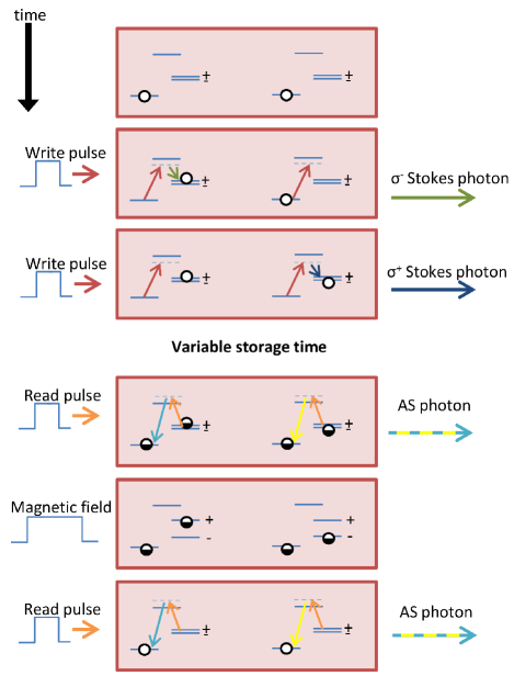
Figure 1: Schematics of the experiment. Each of the two atoms shown represents one of the N states in the sum of the Dicke state.

Immediately after the pumping, a weak and short write pulse with a circular $\sigma^{+}$ polarization is applied to the ensemble. The laser detuning should be large enough in order for the main atom light interaction to be a spontaneous Raman transition to the $\left|s\right\rangle$ state. Since the circular polarization dictates a transition to the Zeeman sublevel $\left|e,m_{s}=0\right\rangle$, the spontaneous Raman decay can be to levels $\left|s,m_{s}=0,\pm 1\right\rangle$, but since $\textup{F}=\textup{F}^{\prime}$ the transition to $\left|s,m_{s}=0\right\rangle$ is forbidden and the other two sublevels have the same probability Vurgaftman and Bashkansky . Thus, upon a successful detection of one photon in one of the polarizations $\sigma^{+}$ or $\sigma^{-}$, the spin state of the metastable level will become $\left|s,m_{s}=-1\right\rangle$ or $\left|s,m_{s}=+1\right\rangle$ respectively. If for example the detected photon is $\sigma^{+}$ then the collective state will be

$$\left|\Psi_{s1}\right\rangle=\frac{1}{\sqrt{N}}\sum_{i=1}^{N}e^{i\mathbf{(k_{w}-k_{s})x_{i}}}\left|s_{i}^{-}\right\rangle\left|+_{s}\right\rangle,$$ (2)

where $\left|s_{i}^{-}\right\rangle$ means that the $i$th atom is now at the state $\left|s,m_{s}=-1\right\rangle$ while all other atoms are in the ground $\left|g^{-}\right\rangle$ state. $\left|+_{s}\right\rangle$ means a Stokes photon with $\sigma^{+}$ polarization is emitted, $\mathbf{k_{w}}$ is the write laser wave vector, $\mathbf{k_{s}}$ is the Stokes photon wave vector and $\mathbf{x_{i}}$ is the coordinate of the $i$th atom. The atomic state is in a Dicke-like state Dicke (1954). This is a long lived atomic coherence where the main decoherence process is the atomic motion that can change the phases between the different atomic states Duan et al. (2002). In the following, we will assume no motion, meaning that these phases do not alter during the storage time. In this case, upon applying a read pulse with a perfect phase matching condition $\mathbf{k_{w}}+\mathbf{k_{r}=\mathbf{k_{s}}+\mathbf{k_{as}}}$, a constructive interference in the direction of the AS wave vector will cause this mode to dominate all other directions Sangouard et al. (2011). Thus, in the case of no atomic motion and perfect phase matching, the phase terms just sum up to unity so it is possible to omit them from now on.

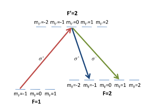
Figure 2: The possible alternatives for single Stokes photon generation during the write process. Red arrow - write beam, Green and blue arrows - Stokes photons.

Now it is possible to quickly repeat the write pulse in order to create another excitation in the metastable state (of course, this pulse will create an excitation only with low probability, but since it is a heralded scheme, we are looking only upon successful events). Let us concentrate on the events where the second Stokes photon that is emitted has the opposite polarization than the first one, thus the collective state will be now

$$\left|\Psi_{s2}\right\rangle=\frac{1}{\sqrt{2N(N-1)}}\sum_{i\neq j=1}^{N}\left|s_{i}^{-}s_{j}^{+}\right\rangle\left|+_{s}-_{s}\right\rangle.$$ (3)

After a certain storage time, a $\sigma^{-}$ polarization read pulse is sent into the media. This pulse can interact with one of the excited Dicke states releasing with some probability one AS photon. There are two possibilities, one that the atoms are in the $\left|s,m_{s}=+1\right\rangle$ state and one that the atoms are in the $\left|s,m_{s}=-1\right\rangle$ state. Each of these options can produce different AS single photons as described in Fig. 3. The AS transition strengths may not be the same due to different Clebsch–Gordan coefficients, thus there is a need to multiply each transition with the proper probability amplitude denoted by $P_{kl}^{(\textup{F})}$ where $k$ is the Zeeman sublevel of the excited state, $l$ is the Zeeman sublevel of the ground state and F is the hyperfine level of the ground state.

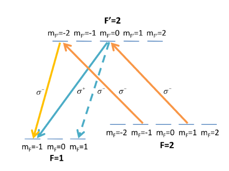
Figure 3: The possible alternatives for single AS photon generation during the read process. orange arrows - read beam, blue, dashed blue and yellow arrows - AS photons.

The AS photon polarization is correlated with the atomic spin level that remains in the ensemble and the state becomes

$${\displaystyle\begin{array}[]{c}\left|\Psi_{as1}^{0}\right\rangle=\frac{1}{\sqrt{2N(N-1)}}{\displaystyle\sum_{i\neq j=1}^{N}}{\scriptstyle P}_{{\scriptscriptstyle 0,1}}^{{\scriptscriptstyle(2)}}\left|s_{i}^{-}\right\rangle({\scriptstyle P}_{{\scriptstyle{\scriptscriptstyle 0,-1}}}^{{\scriptscriptstyle(1)}}\left|\text{g}_{j}^{-}\right\rangle\left|+_{as}\right\rangle\\ +{\scriptstyle P}_{{\scriptscriptstyle 0,1}}^{{\scriptscriptstyle(1)}}\left|\text{g}_{j}^{+}\right\rangle\left|-_{as}\right\rangle)+{\scriptstyle P}_{{\scriptscriptstyle-2,-1}}^{{\scriptscriptstyle(2)}}{\scriptstyle P}_{{\scriptscriptstyle-2,-1}}^{{\scriptscriptstyle(1)}}\left|s_{i}^{+}\right\rangle\left|\text{g}_{j}^{-}\right\rangle\left|-_{as}\right\rangle,\end{array}}$$ (4)

where $\left|\text{g}^{-}\right\rangle$ and $\left|\text{g}^{+}\right\rangle$ are the relaxation of the first AS photon to the Zeeman ground state sublevels $m_{F}=-1$ or $m_{F}=+1$ respectively.

Now a magnetic field is applied to the ensemble creating a Zeeman splitting of the $\left|s\right\rangle$, $\left|g\right\rangle$ states. The two Zeeman levels will acquire a different phase during the single excitation storage time according to the energy splitting. For an energy splitting $\omega_{m}$ in the $\left|s\right\rangle$ level and $\omega_{n}$ in the $\left|g\right\rangle$ level and after a storage time $\tau$ the state will become

$${\textstyle{\scriptstyle\begin{array}[]{l}{\displaystyle\left|\Psi_{as1}^{\tau}\right\rangle={\scriptstyle{\textstyle\frac{1}{\sqrt{2N(N-1)}}}}\sum_{i\neq j=1}^{N}{\scriptstyle P}_{{\scriptscriptstyle 0,1}}^{{\scriptscriptstyle(2)}}e^{-i\omega_{m}\tau}\left|s_{i}^{-}\right\rangle}\\ \;\;\;\;\times{\displaystyle({\scriptstyle P}_{{\scriptscriptstyle 0,-1}}^{{\scriptscriptstyle(1)}}e^{-i\omega_{n}\tau}\left|\text{g}_{j}^{-}\right\rangle\left|+_{as}\right\rangle+{\scriptstyle P}_{{\scriptscriptstyle 0,1}}^{{\scriptscriptstyle(1)}}e^{i\omega_{n}\tau}\left|\text{g}_{j}^{+}\right\rangle\left|-_{as}\right\rangle)}\\ \;\;\;\;{\displaystyle+{\scriptstyle P}_{{\scriptscriptstyle-2,-1}}^{{\scriptscriptstyle(2)}}{\scriptstyle P}_{{\scriptscriptstyle-2,-1}}^{{\scriptscriptstyle(1)}}e^{i(\omega_{m}-\omega_{n})\tau}\left|s_{i}^{+}\right\rangle\left|\text{g}_{j}^{-}\right\rangle\left|-_{as}\right\rangle.}\end{array}}}$$ (5)

Sending another read pulse strong enough to create a second AS photon will produce the following state unity :

$$\begin{array}[]{c}{\textstyle{\displaystyle\left|\Psi_{as2}^{\tau}\right\rangle={\displaystyle{\textstyle\frac{\alpha}{\sqrt{2N(N-1)}}}\sum_{i\neq j=1}^{N}}e^{-i\omega_{m}\tau}{\textstyle\left|\text{g}_{i}^{-}\right\rangle^{{\scriptscriptstyle B}}}\left|-_{as}\right\rangle^{{\scriptscriptstyle B}}({\scriptstyle P}_{{\scriptscriptstyle 0,1}}^{{\scriptscriptstyle(1)}}e^{i\omega_{n}\tau}\left|\text{g}_{j}^{+}\right\rangle^{{\scriptscriptstyle A}}\left|-_{as}\right\rangle^{{\scriptscriptstyle A}}}}+{\scriptstyle P}_{{\scriptscriptstyle 0,-1}}^{{\scriptscriptstyle(1)}}e^{-i\omega_{n}\tau}\left|\text{g}_{j}^{-}\right\rangle^{{\scriptscriptstyle A}}\left|+_{as}\right\rangle^{{\scriptscriptstyle A}})+e^{i(\omega_{m}-\omega_{n})\tau}({\scriptstyle P}_{{\scriptscriptstyle 0,-1}}^{{\scriptscriptstyle(1)}}\left|\text{g}_{i}^{-}\right\rangle^{{\scriptscriptstyle B}}\left|+_{as}\right\rangle^{{\scriptscriptstyle B}}\\ +{\scriptstyle P}_{{\scriptscriptstyle 0,1}}^{{\scriptscriptstyle(1)}}\left|\text{g}_{i}^{+}\right\rangle^{{\scriptscriptstyle B}}\left|-_{as}\right\rangle^{{\scriptscriptstyle B}})\left|\text{g}_{j}^{-}\right\rangle^{{\scriptscriptstyle A}}\left|-_{as}\right\rangle^{{\scriptscriptstyle A}},\end{array}$$ (6)

where the $A,B$ notations represent the emitted AS photon during the first or second read pulse respectively and $\alpha={\scriptstyle P}_{{\scriptscriptstyle 0,1}}^{{\scriptscriptstyle(2)}}{\scriptstyle P}_{{\scriptscriptstyle-2,-1}}^{{\scriptscriptstyle(2)}}{\scriptstyle P}_{{\scriptscriptstyle-2,-1}}^{{\scriptscriptstyle(1)}}$. For simplicity in the following we will abbreviate $\left|-_{as}\right\rangle^{A}\left|-_{as}\right\rangle^{B}\equiv\left|--\right\rangle$ etc., hence the state can be written as

$$\begin{array}[]{c}\left|\Psi_{as2}^{\tau}\right\rangle={\textstyle\frac{\alpha}{\sqrt{2N(N-1)}}{\textstyle{\displaystyle\sum_{i\neq j=1}^{N}}}}e^{-i(\omega_{m}+\omega_{n})\tau}{\scriptstyle P}_{{\scriptscriptstyle 0,-1}}^{{\scriptscriptstyle(1)}}\left|\text{g}_{j}^{-}\text{g}_{i}^{-}\right\rangle\left|+-\right\rangle\\ +e^{-i(\omega_{m}-\omega_{n})\tau}{\scriptstyle P}_{{\scriptscriptstyle 0,1}}^{{\scriptscriptstyle(1)}}\left|\text{g}_{j}^{+}\text{g}_{i}^{-}\right\rangle\left|--\right\rangle\\ +e^{i(\omega_{m}-\omega_{n})\tau}{\scriptstyle P}_{{\scriptscriptstyle 0,-1}}^{{\scriptscriptstyle(1)}}\left|\text{g}_{j}^{-}\text{g}_{i}^{-}\right\rangle\left|-+\right\rangle\\ +e^{i(\omega_{m}-\omega_{n})\tau}{\scriptstyle P}_{{\scriptscriptstyle 0,1}}^{{\scriptscriptstyle(1)}}\left|\text{g}_{j}^{-}\text{g}_{i}^{+}\right\rangle\left|--\right\rangle.\end{array}$$ (7)

Since there is a sum over all the ensemble, the time ordering may be switched and different indices for the atoms can be dropped. As $\left|\text{g}^{-}\right\rangle$ is just the ground state it can be omitted from the equation and we get

$$\begin{array}[]{c}\left|\Psi_{as2}^{\tau}\right\rangle=2\alpha{\scriptstyle P}_{{\scriptscriptstyle 0,1}}^{{\scriptscriptstyle(1)}}\cos[(\omega_{m}-\omega_{n})\tau]\left|--\right\rangle{\textstyle{\displaystyle(\frac{1}{N}\sum_{i=1}^{N}}}\left|\text{g}_{i}^{+}\right\rangle)\\ +\alpha{\scriptstyle P}_{{\scriptscriptstyle 0,-1}}^{{\scriptscriptstyle(1)}}(e^{i(\omega_{m}-\omega_{n})\tau}\left|-+\right\rangle+e^{-i(\omega_{m}+\omega_{n})\tau}\left|+-\right\rangle).\end{array}$$ (8)

Let us normalize the state for every storage time, thus the normalized state will be (taking into account that $P_{{\scriptscriptstyle 0,1}}^{{\scriptscriptstyle(1)}}=P_{{\scriptscriptstyle 0,-1}}^{{\scriptscriptstyle(1)}}$)

$$\begin{array}[]{l}\left|\Psi_{as2}^{\tau}\right\rangle=\sqrt{2}\frac{\cos[(\omega_{m}-\omega_{n})\tau]}{\sqrt{2\cos^{2}[(\omega_{m}-\omega_{n})\tau]+1}}\left|--\right\rangle{\textstyle({\displaystyle\frac{1}{N}\sum_{i=1}^{N}}}\left|\text{g}_{i}^{+}\right\rangle)\\ +\frac{1}{\sqrt{2}}\frac{1}{\sqrt{2\cos^{2}[(\omega_{m}-\omega_{n})\tau]+1}}\left(e^{i(\omega_{m}-\omega_{n})\tau}\left|-+\right\rangle+e^{-i(\omega_{m}+\omega_{n})\tau}\left|+-\right\rangle\right).\end{array}$$ (9)

The second term is actually a generalized Bell state. The most interesting case will be for storage time where the phase is $(\omega_{m}-\omega_{n})\tau=\nicefrac{\mathrm{\pi}}{\mathrm{2}}$. In this case the first term vanishes and the photonic state is just a rotated maximally entangled Bell state $\left|\Psi^{\prime}\right\rangle=\frac{1}{\sqrt{2}}\left(\left|-+\right\rangle+e^{i\phi}\left|+-\right\rangle\right)$.

III Practical issues

The previous section dealt with an ideal case. For real applications there are a few issues that needs to be answered regarding the scheme we presented. The main two issues are the coherence time and the fidelity of the process.

III.1 Coherence

In order for the scheme to succeed the coherence time of the collective state of the atoms should be much longer than the experiment time. A typical coherence can reach up to 1 ms in cold atoms and a few hundred $\mu s$ in warm vapor Zhao et al. (2008a). In warm vapor the spatial coherence of the collective spin state limits the lifetime. Measurements in Rubidium of single photon storage reveal a quantum nature up to 5 $\mu s$ Bashkansky et al. (2012). For a 0.1 $\mu s$ time storage with magnetic field, the frequency shift for substantial phase shift will be on the order of 10 MHz meaning a magnetic field of $\sim$10 G. Switching on and off such a field with a 100 ns time scale is achievable.

III.2 Fidelity

The fidelity of the entangled state is affected by three major contributions. The first one is having more than one excited Stokes/anti Stokes photon per write/read pulse, the second one is the detection efficiency and the third one is the detector’s dark counts Sangouard et al. (2011). In general, for spontaneous Raman scattering the state after a write pulse can be written as

$$\begin{array}[]{c}\left|\Psi\right\rangle=\sqrt{P_{\lambda}(0)}\left|e\right\rangle\left|0_{s}\right\rangle+\sqrt{P_{\lambda}(1)}\frac{1}{\sqrt{N}}\sum_{i=1}^{N}\left|s_{i}\right\rangle\left|1_{s}\right\rangle\\ +\sqrt{P_{\lambda}(2)}\frac{1}{N}\sum_{i=1}^{N}\sum_{j=1}^{N}\left|s_{i}s_{j}\right\rangle\left|2_{s}\right\rangle+....,\end{array}$$ (10)

where $P_{\lambda}(n)$ is the probability of exciting $n$ atoms in the specific mode and $\left|n_{s}\right\rangle$ is a state with $n$ Stokes photons. For low excitation number each excitation is independent, thus this probability will have a Poisson distribution defined by parameter $\lambda$, which is the average excitation number. In order to have only a single excitation, at most, due to each write pulse we need to use a weak pulse such that $P_{\lambda}(0)\gg P_{\lambda}(1)\gg P_{\lambda}(2)$. Moreover, each photon is detected with a lower probability due to detectors efficiencies, fiber couplings, and filters. Two Stokes photons can be produced via two processes: two photons in one of the pulses and zero in the second and one photon in each write pulse. For our experiment both options are fine, as long as the creation of three photons will be negligible. Since the process of creating N Stokes photons is a Poisson process, we can calculate the probability of two and three photons events using the probability of a one photon event. We note also that lower detection efficiency may cause three photons to be detected as two, for example. In the case two photons are created the probability to detect them is of course dependent upon the detection efficiency $P_{detect}$ and will be in our case $P_{det}(2\text{,}2)=P_{\lambda}(2)\times P_{detect}^{2}$. The probability of detecting only two photons while exciting $n$ atoms will be $P_{det}(n\text{,}2)=\left(\begin{array}[]{c}n\\ 2\end{array}\right)\times P_{\lambda}(n)\times P_{detect}^{2}\times(1-P_{detect})^{n-2}$. Dark counts also contribute to lower the fidelity by adding a false detected photon. The probability for one dark count per pulse up to first order will be $P_{dark}(1)=P_{\lambda}(0)\times P_{dc}+P_{\lambda}(1)\times(1-P_{detect})\times P_{dc}$, where $P_{dc}$ is the probability for a dark count per pulse that is related to the length of the pulse.

In order to quantify the total fidelity of the state created and the rate of successful events we assume a post selected measurement where we measure one AS photon after each read pulse. In this case a successful event is regarded as an event where two Stokes photons are created and detected with different polarization, thus the probability of such an event is $P_{succes}=P_{det}(2,2)$. False events are all the events with excitation number $n\neq 2$ that lead to a detection of two Stokes photons. Figure 4 shows the probabilities of false and successful events as a function of the Poisson parameter. Here we take a detection efficiency of $P_{detect}=75\%$ and dark counts rate of 10 Hz Eisaman et al. (2011), thus for a 100 ns pulse $P_{dc}=10^{-6}$. The fidelity can be taken as the ratio between false and successful probabilities, thus a fidelity of 95% is achievable using a Poisson parameter $\lambda=0.2$.

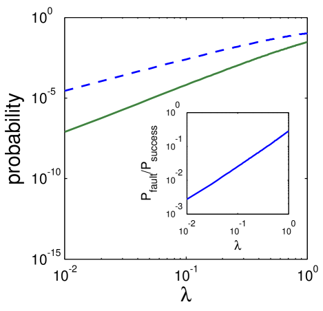
Figure 4: Probability for a successful and false events as a function of the Poisson parameter (blue - successful event, green - false event). The calculation uses dark counts probability of $10^{-6}$ and detection efficiency of 75%. Inset shows the ratio between the events probabilities.

Figure 5 presents the probabilities of the main false events. The predominant false events in low $\lambda$ are dark counts in the detector while high $\lambda$ suffers mostly from events related to false detection of higher excitation modes due to the imperfect detection efficiency. It is important to notice that there is a trade off between maximizing the rate of successful events (larger $\lambda$) and minimizing the false detection of higher events (smaller $\lambda$).

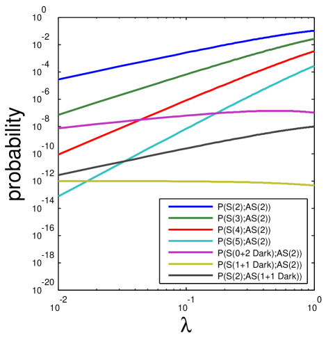
Figure 5: Probabilities of the main events that can contribute to a post selected experiment when two Stokes photons and two AS photons are detected. The notation P(S(n);AS(m)) represents the actual number of photons + dark counts that are created in the experiment. P(S(2);AS(2)) is a successful event, while all others contribute to false events. The sum of all these false events is shown in Fig. 4.

The possible rate of a two photon entanglement source (disregarding the detection efficiency of the AS photon) can be estimated by calculating the potential probability for a successful experiment which is $\frac{1}{2}\times P_{det}(2,2,\lambda=0.2)\times(P_{B}(1))^{2}\approx 10^{-3}$, where the half is due to detections of $\left|+_{s}+_{s}\right\rangle/\left|-_{s}-_{s}\right\rangle$ and $P_{B}(1)=0.5$ is the optimal probability for one AS emission according to Binomial distribution with a total of two excitations. This ensures maximal rate for the read process. This probability will create an entangled pair with Fidelity of 95%. Assuming a repetition rate of 10 MHz, bounded by pumping rate due to the natural lifetime of the atoms, the successful experiment rate will be $\sim$10 kHz. This calculation takes into account the best up to date detectors, with minimal fiber coupling losses. A more conventional setup may have lower detection efficiencies of $\sim$30%. This will lower the rate substantially to $\sim$100 Hz for the same fidelity. The tremendous progress in the field of single photon detection Eisaman et al. (2011) implies that even higher rates will be possible in the near future.

IV Conclusions

A scheme for the creation of a polarization entanglement between two photons using atomic ensemble was presented. This scheme relies on the fact that optical transitions between Zeeman sublevels in the single photon regime may act as a polarization beam splitter. Taking experimental restrictions to consideration we estimate a fidelity that can reach up to 95% with entangled pair production rate of 10 kHz. Combined with the ability to store the photons as a polariton in the ensemble this scheme has the potential to become a useful source for quantum communication beyond current available sources.

Acknowlegments

We acknowledge the support of ISF Bikura grant no. 1567/12. A. Retzker also acknowledge the support of carrier integration grant(CIG) no. 321798 IonQuanSense FP7-PEOPLE-2012-CIG.

References

- Pan et al. (2012) J.-W. Pan, Z.-B. Chen, C.-Y. Lu, H. Weinfurter, A. Zeilinger, and M. Żukowski, Rev. Mod. Phys. 84, 777 (2012).
- Horodecki et al. (2009) R. Horodecki, M. Horodecki, and K. Horodecki, Rev. Mod. Phys. 81, 865 (2009).
- Aspect et al. (1981) A. Aspect, P. Grangier, and G. Roger, Phys. Rev. Lett. 47, 460 (1981).
- Kwiat et al. (1995) P. G. Kwiat, K. Mattle, H. Weinfurter, A. Zeilinger, A. V. Sergienko, and Y. Shih, Phys. Rev. Lett. 75, 4337 (1995).
- Kwiat et al. (1993) P. G. Kwiat, A. M. Steinberg, and R. Y. Chiao, Phys. Rev. A 47, R2472 (1993).
- Eisaman et al. (2011) M. D. Eisaman, J. Fan, a. Migdall, and S. V. Polyakov, Rev. Sci. Instrum. 82, 071101 (2011).
- Kuhn et al. (2002) A. Kuhn, M. Hennrich, and G. Rempe, Phys. Rev. Lett. 89, 067901 (2002).
- Duan et al. (2001) L. M. Duan, M. D. Lukin, I. Cirac, and P. Zoller, Nature 414, 413 (2001).
- Sangouard et al. (2011) N. Sangouard, C. Simon, H. de Riedmatten, and N. Gisin, Rev. Mod. Phys. 83, 33 (2011) .
- Zhao et al. (2008a) B. Zhao, Y.-A. Chen, X.-H. Bao, T. Strassel, C.-S. Chuu, X.-M. Jin, J. Schmiedmayer, Z.-S. Yuan, S. Chen, and J.-W. Pan, Nature Phys. 5, 95 (2008a).
- Zhao et al. (2008b) R. Zhao, Y. O. Dudin, S. D. Jenkins, C. J. Campbell, D. N. Matsukevich, T. B. Kennedy, and A. Kuzmich, Nature Phys. 5, 100 (2008b).
- van der Wal et al. (2003) C. H. van der Wal, M. D. Eisaman, A. André, R. L. Walsworth, D. F. Phillips, a. Zibrov, and M. D. Lukin, Science 301, 196 (2003).
- Bashkansky et al. (2012) M. Bashkansky, F. K. Fatemi, and I. Vurgaftman, Opt. Lett. 37, 142 (2012).
- Dai et al. (2012) H.-N. Dai, H. Zhang, S.-J. Yang, T.-M. Zhao, J. Rui, Y.-J. Deng, L. Li, N.-L. Liu, S. Chen, X.-H. Bao, X.-M. Jin, B. Zhao, and J.-W. Pan, Phys. Rev. Lett. 108, 210501 (2012).
- Choi et al. (2008) K. S. Choi, H. Deng, J. Laurat, and H. J. Kimble, Nature 452, 67 (2008).
- Akopian et al. (2006) N. Akopian, N. H. Lindner, E. Poem, Y. Berlatzky, J. Avron, D. Gershoni, B. D. Gerardot, and P. M. Petroff, Phys. Rev. Lett. 96, 130501 (2006).
- Stevenson et al. (2006) R. M. Stevenson, R. J. Young, P. Atkinson, K. Cooper, D. A. Ritchie, and A. J. Shields, Nature 439, 179 (2006).
- Gheri et al. (1998) K. M. Gheri, C. Saavedra, P. Törmä, J. I. Cirac, and P. Zoller, Phys. Rev. A 58, R2627 (1998).
- Srivathsan et al. (2013) B. Srivathsan, G. K. Gulati, B. Chng, G. Maslennikov, and D. Matsukevich, and C. Kurtsiefer, Phys. Rev. Lett. 111, 123602 (2013).
- MacRae et al. (2012) A. MacRae, T. Brannan, R. Achal, and A. I. Lvovsky, Phys. Rev. Lett. 109, 033601 (2012).
- Porras and Cirac (2008) D. Porras and J. I. Cirac, Phys. Rev. A 78, 053816 (2008).
- Nielsen and Mø lmer (2010) A. E. B. Nielsen and K. Mø lmer, Phys. Rev. A 81, 043822 (2010).
- Walther et al. (2007) P. Walther, M. D. Eisaman, A. André, F. Massou, M. Fleischhauer, A. S. Zibrov, and M. D. Lukin, Int. J. Quantum Inf. 05, 51 (2007).
- (24) In real schemes the probability for the two polarizations can be different due to spontaneous Raman emission from a second hyperfine excited level. Effectively, it lowers the rate of entanglement creation, but does not harm the fidelity of the state. For more details see I. Vurgaftman and M. Bashkansky, Phys. Rev. A 87, 063836 (2013).
- Dicke (1954) R. H. Dicke, Phys. Rev. 93, 99 (1954).
- Duan et al. (2002) L. M. Duan, J. I. Cirac, and P. Zoller, Phys. Rev. A66, 023818 (2002).
- (27) We assume here that the AS photon extraction probability is sufficiently bellow unity. If this is not the case, corrections are needed for eq. (6) due to a breaking of the symmetry between the extraction probabilities of the first and the second AS photons and the final state is no longer maximally entangled.