One-dimensional Bose–Hubbard model with local three-body interactions

Abstract

We employ the (dynamical) density matrix renormalization group technique to investigate the ground-state properties of the Bose–Hubbard model with nearest-neighbor transfer amplitudes $t$ and local two-body and three-body repulsion of strength $U$ and $W$, respectively. We determine the phase boundaries between the Mott-insulating and superfluid phases for the lowest two Mott lobes from the chemical potentials. We calculate the tips of the Mott lobes from the Tomonaga–Luttinger liquid parameter and confirm the positions of the Kosterlitz–Thouless points from the von Neumann entanglement entropy. We find that physical quantities in the second Mott lobe such as the gap and the dynamical structure factor scale almost perfectly in $t/(U+W)$, even close to the Mott transition. Strong-coupling perturbation theory shows that there is no true scaling but deviations from it are quantitatively small in the strong-coupling limit. This observation should remain true in higher dimensions and for not too large attractive three-body interactions.

I Introduction

The revolutionary control over ultracold atoms in optical lattices made possible the direct experimental observation of many-body states of different quantum systems BDZ08 . Tuning two-body interactions by using Feshbach resonances or changing the strength of the lattice confinement permitted the observation of a superfluid (SF) to Mott-insulating (MI) quantum phase transition for bosonic lattice atoms GMEHB02 for integer densities. More recently, the importance of multi-body interactions has been inferred from experiment WBSHLB10 ; MHLDDN11 . These interactions were so far deemed negligible higher-order many-body interactions.

The minimal model to describe bosonic lattice quantum gases is the Bose–Hubbard model. On a chain with $L$ sites, the Hamilton operator with local two-body and three-body interactions is given by

$$H = -t\hat{T}+U\hat{D}+W\hat{W}\;,$$

$$\hat{T} = \sum_{j=1}^{L-1}\left(\hat{b}_{j}^{\dagger}\hat{b}_{j+1}^{\phantom{\dagger}}+\hat{b}_{j+1}^{\dagger}\hat{b}_{j}^{\phantom{\dagger}}\right)\;,$$

$$\hat{D} = \frac{1}{2}\sum_{j=1}^{L}\hat{n}_{j}(\hat{n}_{j}-1)\;,$$

$$\hat{W} = \frac{1}{6}\sum_{j=1}^{L}\hat{n}_{j}(\hat{n}_{j}-1)(\hat{n}_{j}-2)\;,$$ (1)

where $\hat{b}_{j}^{\dagger}$ and $\hat{b}_{j}^{\phantom{\dagger}}$ are the creation and annihilation operators for bosons on site $j$, $\hat{n}_{j}=\hat{b}_{j}^{\dagger}\hat{b}_{j}^{\phantom{\dagger}}$ is the boson number operator on site $j$, $t$ is the tunnel amplitude between neighboring lattice sites, and $U>0$ ($W>0$) denote the strength of the on-site two-body (three-body) repulsion. There are $N=\rho L$ bosons in the system.

The Bose–Hubbard model in one dimension with pure two-body interactions has been extensively studied KM98 ; KWM00 ; EFG11 ; EFGMKAL12 , using the density matrix renormalization group (DMRG) technique Wh92 . SF-to-MI quantum phase transition points can be determined accurately from the finite-size scaling of the Tomonaga–Luttinger liquid (TLL) parameter $K_{b}$; the model is in the universality class of the spin-1/2 $XY$ model so that there exists a Kosterlitz-Thouless transition in the thermodynamic limit, $L\to\infty$, where $K_{b}=1/2$.

The model including the three-body local interaction remains largely unexplored. The first Mott lobe was recently studied using DMRG SS11 and the cluster expansion approach VM12 . The whole ground-state phase diagram for the first and second lobes was derived from exact diagonalization results for small system sizes $L\leq 8$ So12 and DMRG data for larger system sizes SDMPD12 . Very recently, Sowińsky et al. SCDTL13 studied the full model with attractive two-body and repulsive three-body interactions using the DMRG.

In this work, we examine the static and dynamical ground-state properties of the Bose–Hubbard model with two-body and three-body interactions using large-scale DMRG calculations. To determine the phase boundaries between MI and SF phases we compute the chemical potential, the Tomonaga–Luttinger liquid (TLL) parameter, and the von Neumann entanglement entropy. Moreover, for $\rho=2$, we calculate the single-particle gap and the dynamical structure factor $S(q,\omega)$ using the dynamical DMRG (DDMRG) procedure Je02b .

We find that the three-body interaction is qualitatively irrelevant in one dimension for strong coupling. Its quantitative corrections for $\rho=2$ for the size of the Mott lobe, the gap, and the dynamical structure factor can be incorporated almost perfectly by rescaling $t/U\to t/(U+W)$ in the results for a bare two-body interaction ($W=0$). Strong-coupling perturbation theory shows that this rescaling is not rigorous but quantitative corrections are very small for strong interactions.

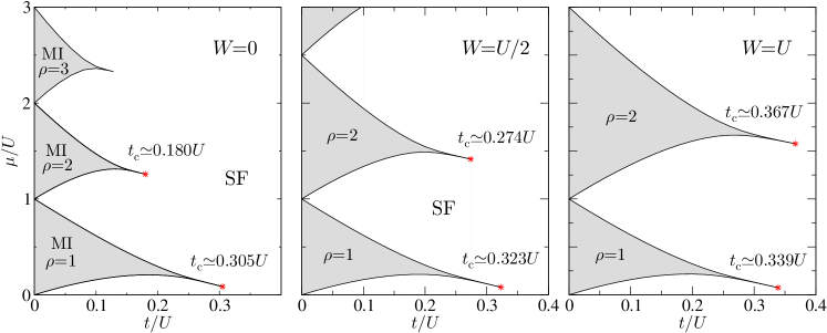
Figure 1: (Color online) Ground-state phase diagram of the one-dimensional Bose–Hubbard model with three-body interactions for $W=0$ (left panel), $W=U/2$ (middle panel), and $W=U$ (right panel), showing superfluid (SF) and Mott insulating (MI) regions as a function of the chemical potential $\mu/U$ and the electron transfer amplitude $t/U$. Results are based on DMRG data for lattices with up to $L=128$ sites and open boundary conditions. The position of the Mott tips is obtained from the finite-size extrapolation of the Tomonaga–Luttinger parameter $K_{b}(L)$, eq. (4).

II Ground-state phase diagram

II.1 Single-particle gap

The Mott-insulating phases are characterized by a finite gap for single-particle excitations. The chemical potential $\mu(L,N)$ gives the energy for adding the $N$th particle to the system with $L$ sites in its ground state,

$$\mu(L,N)=E_{0}(L,N)-E_{0}(L,N-1)\;,$$ (2)

where $E_{0}(L,N)$ is the ground-state energy for $N$ bosons on $L$ sites. For $t=0$, $[\mu(L,L+1)=U,\mu(L,L)=0]$ and $[\mu(L,2L+1)=2U+W,\mu(L,2L)=U]$ hold. The single-particle gap results from the difference between the chemical potentials for $N+1$ and $N$ particles,

$$\Delta(L,N)=\mu(L,N+1)-\mu(L,N)\;.$$ (3)

In the Mott insulating state, the gap remains finite in the thermodynamic limit, $\Delta(\rho)\equiv\Delta(L\to\infty,N\to\infty)>0$ for fixed $\rho=N/L$. In the superfluid phase, the chemical potential is a continuous function of the density $\rho$. For $t=0$, we have $\Delta(\rho=1)=U$ and $\Delta(\rho=2)=U+W$.

For integer fillings $\rho$ and for large $U/t$, the Bose–Hubbard model is in its Mott insulating phase. Thus, the ground-state phase diagram in the plane $(t/U,\mu/U)$ shows superfluid and Mott-insulating regions, see Fig. 1. In the shaded regions, the particle density is constant and the gap for fixed $t/U$ is given by the difference in the chemical potentials at the boundaries to the superfluid phases, i.e., the chemical potentials determine the phase boundaries. Unfortunately, the gaps become exponentially small close to the critical points $t_{\rm c}^{\rho}$ above which the Mott gap is zero. Since it is not possible to resolve such small gaps numerically, the critical points must be determined in a different manner, see Sect. II.2. We obtained the ground-state phase diagram in Fig. 1 using the DMRG method with up to $L=128$ sites and open boundary conditions (OBCs). We extrapolated the chemical potentials to the thermodynamical limit using a second-order polynomial fit in $1/L$ for $\mu(L,L+1)$ and $\mu(L,L)$ EFG11 ; EFGMKAL12 .

In the absence of the three-body interaction (left panel), the Mott lobes become smaller with increasing density $\rho$, and, concomitantly, the values of the transition points $t_{\rm c}^{\rho}$ decrease with increasing $\rho$. When we switch on the three-body interaction (middle panel for $W=U/2$, right panel for $U=W$), the first Mott lobe is almost unchanged in comparison with the result for $W=0$, and the dependence of $t_{\rm c}^{\rho=1}$ on $W$ is rather weak, too. This is readily understood because at $t_{\rm c}^{\rho=1}\simeq 0.3U$, there are few doubly occupied sites in the ground state and hardly any triply occupied sites: the Mott transition occurs at strong coupling where triple occupancies are strongly reduced for $\rho=1$. The situations is different for $N=2L$ particles because there are essentially double and triple occupancies present at the transition so that the three-body interaction is effective. Therefore, the size of the second Mott lobe and the value of $t_{\rm c}^{\rho=2}$ substantially increase as a function of $W$, which also pushes up in energy the other Mott lobes.

II.2 Critical interactions

In order to determine the transition points, we compute the TLL parameter $K_{b}$ in the superfluid phase. The Fourier transformation of the static structure factor, $S(q)=(1/L)\sum_{j,l}e^{{\rm i}q(j-l)}(\langle\hat{n}_{j}\hat{n}_{l}\rangle-\langle\hat{n}_{j}\rangle\langle\hat{n}_{l}\rangle)$ at $q=2\pi/L$ defines $K_{b}(L)$ EGN05 ; EFG11 ,

$$\frac{1}{2\pi K_{b}(L)}=\frac{S(2\pi/L)}{2\pi/L}\;.$$ (4)

The TLL exponent is then obtained from the extrapolation of the DMRG data, $K_{b}=\lim_{L\to\infty}K_{b}(L)$. At the SF-MI transition point we expect that $K_{b}=1/2$ Gi03 , as in the case for the model (1) at $W=0$ KM98 ; KWM00 ; EFG11 . In this way, the transition points $t_{\rm c}^{\rho}$ can be determined accurately.

In the upper panels of Fig. 2 we demonstrate the finite-size scaling of the TLL parameter $K_{b}(L)$ for $\rho=1$ (left panel) and $\rho=2$ (right panel) at $U=W$, where we use the DMRG method with up to $L=512$ sites and OBC. The transition points are determined from $\lim_{L\to\infty}K_{b}(L)=0.5$ as $t_{\rm c}^{\rho=1}=0.339\pm 0.001$ and $t_{\rm c}^{\rho=2}=0.367\pm 0.001$. Our data improve the estimates from the exact diagonalization method So12 with up to $L=8$ sites, $t_{{\rm c},{\rm ED}}^{\rho=1}/U=0.32$ and $t_{{\rm c},{\rm ED}}^{\rho=2}/U=0.38$.

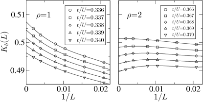
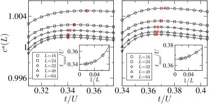
Figure 2: (Color online) DMRG data for the Tomonaga–Luttinger liquid parameter $K_{b}(L)$ (upper panels) and the central charge $c^{\ast}(L)$ (lower panels) for the first (left panels) and second (right panels) Mott lobes in the model (1) for $W/U=1$. The position of the maxima of $c^{\ast}(L)$ can be extrapolated systematically to the thermodynamic limit, as shown in the insets of the lower panels.

In order to confirm the values of the critical points, we address the von Neumann entanglement entropy $S_{L}(\ell)$, defined as $S_{L}(\ell)=-{\rm Tr}_{\ell}(\rho_{\ell}\ln\rho_{\ell})$ with the reduced density matrix $\rho_{\ell}={\rm Tr}_{L-\ell}(\rho)$. For a system with central charge $c$, one finds for periodic boundary conditions (PBCs) CC04

$$S_{L}(\ell)=\frac{c}{3}\ln\left[\frac{L}{\pi}\sin\left(\frac{\pi\ell}{L}\right)\right]+s_{1}\;,$$ (5)

where $s_{1}$ is a non-universal constant and corrections are small, of the order $1/L$. The constant $s_{1}$ can be eliminated by subtracting $S_{L}(L/2)$ from $S_{L}(L/2-1)$ so that we can define the size-dependent central charge Ni11

$$c^{*}(L)=\frac{3\left[S_{L}(L/2-1)-S_{L}(L/2)\right]}{\ln\left[\cos(\pi/L)\right]}\;.$$ (6)

Since the excitations of the interacting suprafluid in one dimension form a TLL with central charge $c=1$, we can use $c^{*}=\lim_{L\to\infty}c^{*}(L)$ to locate the critical interactions.

In the lower panels of Fig. 2, we employ the DMRG method for up to $L=64$ sites and PBCs. As in the case of the model (1) for $W/U=0$ EFGMKAL12 , $c^{\ast}(L)$ displays maxima as a function of the hopping amplitude $t/U$ for fixed system size $L$. When we extrapolate the position of the maxima in $c^{\ast}(L)$ for $U=W$ to the thermodynamic limit, we obtain the transition points as $t_{\rm c}^{\rho=1}/U=0.340\pm 0.002$ and $t_{\rm c}^{\rho=2}/U\simeq 0.366\pm 0.002$, in excellent agreement with our previous estimate from the TLL parameter $K_{b}$. In this way, we reliably determined the position of the tips in the Mott lobes of the ground-state phase diagram in Fig. 1.

III Second Mott lobe

In the remainder of this work we focus on the second Mott lobe, $\rho=2$ and $t<t_{\rm c}^{\rho=2}$, where the three-body repulsion plays a significant role.

III.1 Gap function

For strong interactions, the gap can be calculated systematically in a power series in the particle hopping. For $N=2L+1$ particles, the first non-trivial order describes the free propagation of a triple occupancy so that its dispersion relation is given by $\omega^{+}(k)=E^{+}(k)-E_{0}(L,2L)=W+2U-6t\cos(k)$. For $N=2L-1$ particles, the singly occupied site (a hole in the background of doubly occupied sites) has the dispersion relation $\omega^{-}(k)=E^{-}(k)-E_{0}(L,2L)=-U+4t\cos(k)$. Therefore, to leading order in $t$, the gap becomes $\Delta={\rm Max}_{k}[\omega^{+}(k)-\omega^{-}(k)]$ or

$$\frac{\Delta(t\ll U,W)}{U+W}=1-\frac{10t}{U+W}+\ldots$$ (7)

To leading order, $\Delta$ is only a function of $t/(U+W)$. In the left panel of Fig. 3 we plot $\Delta/(U+W)$ as a function of $t/(U+W)$ for $t<t_{\rm c}^{\rho=2}$. It is seen that the data for $W=0,U/2,U$ essentially collapse onto a single curve, suggesting that the gap is solely a function of $U+W$. Likewise, when we plot the modified chemical potentials $\mu+W$ as a function of $t/(U+W)$ in the right panel of Fig. 3, we see that the second Mott lobes for $W=0,U/2,U$ almost collapse onto each other. Deviations are visible only close to the transition points.

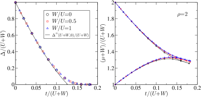
Figure 3: (Color online) Rescaled single-particle gaps (left panel) and phase diagram (right panel) of the second Mott lobe ($\rho=2$) in the model (1). The data for $W=0,U/2,U$ collapse onto each other. Also shown is the third-order result for the gap $\Delta^{(3)}(U+W,0)$ at $U=W$, eq. (III.3.1).

III.2 Dynamical structure factor

The dynamical structure factor $S(q,\omega)$ characterizes the density-density response of the Bose gas and is directly accessible by Bragg spectroscopy SICSPK99 ; EGKPLPS09 . It is defined as

$$S(q,\omega)=\sum_{n}|\langle\psi_{n}|\hat{n}(q)|\psi_{0}\rangle|^{2}\delta(\omega-\omega_{n}),$$ (8)

where $\hat{n}(q)=\sum_{l}e^{{\rm i}ql}\hat{b}_{l}^{\dagger}\hat{b}_{l}^{\vphantom{\dagger}}$, $|\psi_{0}\rangle$ and $|\psi_{n}\rangle$ denote the ground state and $n$th excited state, respectively, and $\omega_{n}=E_{n}-E_{0}$ gives the corresponding excitation energy. As shown in Ref. EFG12 ; EFGMKAL12 , we can compute the Lorentz-broadened $S_{\eta}(q,\omega)$ with

$$S_{\eta}(q,\omega)=\int_{-\infty}^{\infty}{\rm d}\omega^{\prime}S(q,\omega^{\prime})\frac{\eta}{\pi[(\omega-\omega^{\prime})^{2}+\eta^{2}]}$$ (9)

for Bose–Hubbard models using the DDMRG technique. In this work, we use $\eta=2t$ for $L=32$ sites with PBCs to obtain smooth curves. Note that the unbroadened dynamical quantities corresponding to the experimental measurements can be extracted from the deconvolution of the DDMRG data as demonstrated in Ref. NGJ04 .

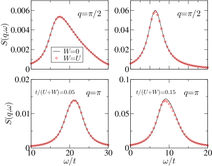
Figure 4: (Color online) Dynamical structure factor $S_{\eta}(q,\omega)$ with Lorentz broadening $\eta=2t$ at momenta $q=\pi/2$ (upper panels) and $q=\pi$ (lower panels) of the second Mott lobe in the model (1) for $t/(U+W)=0.05$ (left panels) and $t/(U+W)=0.15$ (right panels), as obtained from the DDMRG technique for $L=32$ sites.

In Fig. 4 we show $S_{\eta}(q,\omega)$ for $q=\pi/2$ (upper panels) and $q=\pi$ (lower panels) for $t/(U+W)=0.05$ (left panels) and $t/(U+W)=0.15$ (right panels) as a function of $\omega/t$. The results for $W=U$ lie essentially on top of those for $W=0$, apart from small deviations around $\omega=0$ for $t/(U+W)=0.15$ and $q=\pi$, suggesting again a scaling relation.

III.3 Strong-coupling perturbation theory

The strong-coupling analysis of Harris and Lange as used in EFGMKAL12 starts from the unperturbed Hamiltonian $\hat{H}_{0}=U\hat{D}$ where $\hat{D}$ counts the number $n_{D}$ of pair interactions. The perturbation expansion for $t/U\to 0$ relies on the fact that the subspaces with $n_{D}=0,1,2,\ldots$ are well separated. In the presence of the triple interaction $\hat{W}$, we assume energetically separated subspaces for $\hat{H}_{0}=U\hat{D}+W\hat{W}$ that have the unperturbed energies $E_{0}(n_{D},n_{W})=Un_{D}+Wn_{W}$ with two integer quantum numbers $(n_{D}\geq 0,n_{W}\geq 0)$. A transfer process between neighbors with positive integer occupancies $(n_{1}=\rho+m,n_{2}=\rho+n)$ to $(n_{1}=\rho+m-1,n_{2}=\rho+n+1)$ results in an energy transfer

$$\Delta E(m,n)=(n-m+1)\left[U+W(\rho-1)+W(n+m)/2\right]\;.$$ (10)

For $\rho=2$, the resulting finite energy denominators in a perturbation expansion thus include the energies $U+W+W(n+m)/2$. Therefore, there cannot be a rigorous scaling relation, i.e., the physical quantities are not solely a function of $t/(U+W)$.

However, the lowest-order terms involve small deviations from $\rho=2$, i.e., only $(m=0,n=0)$ and $(m=\pm 1,n=\mp 1)$ appear. Thus, only the energy denominator $U+W$ occurs in low-order perturbation theory in $\hat{T}$. Moreover, in higher orders, those terms that involve $t/(U+W)$ have a higher weight than those that are proportional to $t/(2U+W)$ or else. For these practical reasons, the results for the gap and the dynamical structure factor show fairly small deviations from a scaling behavior, apart from the region close to the MI-to-SF transition.

III.3.1 Gap

To be definite, we address the series expansion of the gap to third order. To this end, we repeat the perturbative expansion EFGMKAL12 ; MuensterMSc whereby we effectively replace the energy denominators $U(n_{D,1}-n_{D,2})$ of states with $n_{D_{1}}$ and $n_{D_{2}}$ double occupancies by the appropriate energy differences $U(n_{D,1}-n_{D,2})+W(n_{W,1}-n_{W,2})$. For $\rho=2$ this leads to

$$\frac{\Delta^{(3)}(U,W)}{U+W} = 1-\frac{10t}{U+W}$$

$$+\frac{2t^{2}\left(26U^{2}+57UW+19W^{2}\right)}{(U+W)^{2}(2U+W)(2U+3W)}$$

$$+\frac{12t^{3}}{(U+W)^{3}(2U+W)^{2}(2U+3W)^{2}}$$

$$\hphantom{+}[40U^{4}+160U^{3}W+230U^{2}W^{2}$$

$$\hphantom{+[}+134UW^{3}+29W^{4}]\;.$$

It is seen that deviations from the scaling of $\Delta/(U+W)$ with $t/(U+W)$ first occur in second order. In order to assess the quantitative effect, we use the result for $W=0$ and define

$$\frac{\Delta^{(3,{\rm sc})}(U,W)}{U+W} = \frac{\Delta^{(3)}(U+W,0)}{U+W}$$

$$= 1-\frac{10t}{U+W}+\frac{13t^{2}}{(U+W)^{2}}+\frac{30t^{3}}{(U+W)^{3}}\,.$$

Then, at $U=W$ we consider

$$\delta^{(3)}(U) = \frac{|\Delta^{(3)}(U,U)-\Delta^{(3,{\rm sc})}(U,U)|}{\Delta^{(3)}(U,U)}$$

$$= \frac{t^{2}(61t+45U)}{2(593t^{3}+510t^{2}U-750tU^{2}+150U^{3})}\;.$$

where, e.g., $\delta^{(3)}(t/0.15)=0.012$. At $U=W$ we find that the relative deviation of the scaling curve for $t/U<0.15$ is about one percent or less, a negligibly small correction. This explains the almost perfect scaling seen in Fig. 3.

III.3.2 Dynamical structure factor

As has been shown in Refs. EFGMKAL12 ; MuensterMSc , the dynamical structure factor in the region of the primary Hubbard band can be obtained from the solution of an effective single-particle problem on a ring that describes the propagation of a ‘hole’ (single occupancy for $\rho=2$) and a ‘particle’ (triple occupancy for $\rho=2$) that move with total momentum $q$. The resulting effective single-particle problem is governed by a kinetic term and a potential whose range is proportional to the order of the expansion.

In the calculation of the structure factor, we need the eigenstates $|q;k\rangle$ of $\overline{k}_{0}$ that describes the free propagation of particles and holes,

$$\overline{k}_{0}|q;k\rangle = (\beta_{q}e^{-{\rm i}k}+\beta_{q}^{*}e^{{\rm i}k})|q;k\rangle\;,$$

$$\beta_{q} = -t[\rho+(\rho+1)e^{{\rm i}q}]\;.$$ (14)

The states $|q\rangle$ that enter the calculation of the structure factor are weighted linear combinations of the states $|q;k\rangle$. Up to second order, these weights are solely a function of $t/(U+W)$ and do not play a role for our discussion.

By definition, the states $|q;k\rangle$ are eigenstates of the kinetic contribution to all orders,

$$\overline{k}_{1}|q;k\rangle = (\alpha+\gamma_{q}e^{-{\rm i}2k}+\gamma_{q}^{*}e^{{\rm i}2k})|q;k\rangle\;,$$

$$\gamma_{q} = -t\frac{t\rho(\rho+1)}{U+(\rho-1)W}(1+e^{{\rm i}2q})\;,$$ (15)

$$\alpha = t\frac{8t\rho(\rho+1)}{U+(\rho-1)W}-t\frac{2t(\rho^{2}-1)}{2U+(2\rho-3)W}$$

$$-t\frac{2t\rho(\rho+2)}{2U+(2\rho-1)W}\;.$$

For $\rho=2$, $\alpha$ is not a function of $t/(U+W)$ alone but also involves terms of different analytical structure.

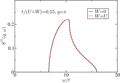
Figure 5: (Color online) Dynamical structure factor in second-order strong-coupling perturbation theory, $S^{(2)}(q=\pi,\omega)$, for $U=W$ and $t/(U+W)=0.15$ (full line), in comparison with the scaling result $S^{(2,{\rm sc})}(q=\pi,\omega)$ (dashed line). The differences are very small.

The same observation holds for the interaction potential. Apart from the hard-core correction that appears when we close the chain into a ring EFGMKAL12 ; MuensterMSc , the interaction potential contains terms between nearest neighbors and next-nearest neighbors of the form

$$\frac{V_{1,1}(q)}{t}=\frac{2t\rho(\rho+1)\cos(q)+2t(2\rho+1)^{2}/3}{U+(\rho-1)W}\;,$$ (16)

and

$$\frac{V_{L-1,1}(q)}{t} = \frac{t\rho(\rho+1)}{U+(\rho-1)W}-\frac{t\rho(\rho+2)}{2U+(2\rho-1)W}$$

$$+\frac{t\rho(\rho+1)e^{-{\rm i}q}}{U+(\rho-1)W}$$

$$+\frac{t\rho(\rho+1)e^{-{\rm i}2q}}{U+(\rho-1)W}-\frac{t(\rho-1)^{2}e^{-{\rm i}2q}}{2U+(2\rho-3)W}\;.$$

The contributions for next-nearest neighbors involve intermediate states with excitation energies that are different from $U+W$ or its multiples for $\rho=2$. In Fig. 5 we show the resulting structure factor to second order $S^{(2)}(q,\omega)$ at $q=\pi$ as a function of $\omega$ for $U=W$, $t/U=0.15$, and $\rho=2$, where we give the full result to second order. For comparison we also show $S^{(2,{\rm sc})}(q,\omega)$ where we replace $U$ by $U+W$ in the results for $W=0$. The quantitative differences are very small so that the scaling $U\to U+W$ is almost fulfilled, as seen in the DDMRG data. Note that the result of $S(q,\omega)$ in Fig. 5 looks quantitatively different from the DDMRG data in the right lower panel of Fig. 4. This is due to the finite broadening width $\eta$ in the DDMRG calculation and the limited validity of the second-order strong-coupling approach for intermediate coupling strengths.

IV Conclusions

In this work we used the numerically exact density matrix renormalization group technique to investigate the one-dimensional Bose–Hubbard model with a two-body interaction $U\hat{D}$ and a three-body interaction $W\hat{W}$. We determined the ground-state phase diagram with and without three-body repulsion for the first and second Mott lobes from the chemical potentials. The calculation of the Tomonaga-Luttinger parameter $K_{b}$ close to the Kosterlitz–Thouless transitions provided accurate estimates for the tips of the Mott lobes where the gaps become exponentially small. We confirmed the results for $t_{\rm c}^{\rho=1,2}$ using the von Neumann entanglement entropy. We find that $t_{\rm c}^{\rho=1}(W)$ increases from $t_{\rm c}^{\rho=1}(0)$ by less than ten percent for $W\leq U$. Moreover, $t_{\rm c}^{\rho=2}(W)$ obeys the relation $t_{\rm c}^{\rho=2}(W)\approx t_{\rm c}^{\rho=2}(0)(1+W/U)$ with an accuracy of a few percent for $W\leq U$.

For the second Mott lobe, $\rho=2$, our numerical data for the gap $\Delta$ and the Lorentz-broadened dynamical structure factor $S_{\eta}(q,\omega)$ showed a similarly good ‘scaling behavior’: the curves for different values of $W=0,U/2,U$ almost fall on top of each other when plotted as a function of $t/(U+W)$. Our results from strong-coupling perturbation theory show that the scaling is not rigorous. However, deviations are quantitatively small because, in the Mott insulating region, interactions are strong so that the physical quantities are largely determined by particle-hole excitations with one triple occupancy and one single occupancy in the background of doubly occupied sites.

Since our observations rely on the strong-coupling picture alone, they should also hold in higher dimensions. The Bose–Hubbard model with pure two-body interactions remains qualitatively correct even in the presence of sizable local three-particle interactions. Of course, this conclusion becomes invalid for substantial attractive three-body interactions that will lead to the formation of local clusters.

- (1) I. Bloch, J. Dalibard, and W. Zwerger, Rev. Mod. Phys. 80, 885 (2008)
- (2) M. Greiner, O. Mandel, T. Esslinger, T. W. Hänsch, and I. Bloch, Nature 415, 39 (2002)
- (3) S. Will, T. Best, U. Schneider, L. Hackermüller, D.-S. Lühmann, and I. Bloch, Nature 465, 197 (2010)
- (4) M. J. Mark, E. Haller, K. Lauber, J. G. Danzl, A. J. Daley, and H.-C. Nägerl, Phys. Rev. Lett. 107, 175301 (2011)
- (5) T. D. Kühner and H. Monien, Phys. Rev. B 58, R14741 (1998)
- (6) T. D. Kühner, S. R. White, and H. Monien, Phys. Rev. B 61, 12474 (2000)
- (7) S. Ejima, H. Fehske, and F. Gebhard, Europhys. Lett. 93, 30002 (2011)
- (8) S. Ejima, H. Fehske, F. Gebhard, K. zu Münster, M. Knap, E. Arrigoni, and W. von der Linden, Phys. Rev. A 85, 053644 (2012)
- (9) S. R. White, Phys. Rev. Lett. 69, 2863 (1992)
- (10) J. Silva-Valencia and A. M. C. Souza, Phys. Rev. A 84, 065601 (2011)
- (11) V. Varma and H. Monien, e-print, arXiv:1211.5664.
- (12) T. Sowiński, Phys. Rev. A 85, 065601 (2012)
- (13) M. Singh, A. Dhar, T. Mishra, R. V. Pai, and B. P. Das, Phys. Rev. A 85, 051604 (2012).
- (14) T. Sowiński, R. W. Chhajlany, O. Dutta, L. Tagliacozzo, and M. Lewenstein, e-print, arXiv:1304.4835.
- (15) E. Jeckelmann, Phys. Rev. B 66, 045114 (2002)
- (16) S. Ejima, F. Gebhard, and S. Nishimoto, Europhys. Lett. 70, 492 (2005)
- (17) T. Giamarchi, Quantum Physics in One Dimension (Clarendon Press, Oxford, 2003)
- (18) P. Calabrese and J. Cardy, J. Stat. Mech.: Theory and Exp. P06002 (2004)
- (19) S. Nishimoto, Phys. Rev. B 84, 195108 (2011)
- (20) J. Stenger, S. Inouye, A. P. Chikkatur, D. M. Stamper-Kurn, D. E. Pritchard, and W. Ketterle, Phys. Rev. Lett. 82, 4569 (1999)
- (21) P. T. Ernst, S. Götze, J. S. Krauser, K. Pyka, D.-S. Lühmann, D. Pfannkuche, and K. Sengstock, Nature Physics 6, 56 (2009)
- (22) S. Ejima, H. Fehske, and F. Gebhard, J. Phys. Conf. Ser. 391, 012031 (2012)
- (23) S. Nishimoto, F. Gebhard, and E. Jeckelmann, J. Phys. Condens. Matter 16, 7063 (2004).
- (24) K. zu Münster, M.Sc. thesis, University of Marburg (2012).