An explicit kernel-split panel-based Nyström scheme for integral equations on axially symmetric surfaces

Abstract

A high-order accurate, explicit kernel-split, panel-based, Fourier–Nyström discretization scheme is developed for integral equations associated with the Helmholtz equation in axially symmetric domains. Extensive incorporation of analytic information about singular integral kernels and on-the-fly computation of nearly singular quadrature rules allow for very high achievable accuracy, also in the evaluation of fields close to the boundary of the computational domain.

1 Introduction

This work is on a high-order accurate panel-based Fourier–Nyström discretization scheme for integral equations associated with the Helmholtz equation in domains bounded by axially symmetric surfaces. Efficient axisymmetric solvers for wave propagation and scattering are important in their own right in optical and microwave applications [22, 30]. They are also needed in multi-particle contexts, for example, to predict the effects of absorption and scattering of sun light from soot in the atmosphere [25].

The present scheme resembles that of Young, Hao, and Martinsson [31]. The main difference lies in the treatment of nearly- and weakly singular oscillatory kernels. In [31], a precomputed 10th order accurate general-purpose Kolm–Rokhlin quadrature [23] is used for discretization in the polar direction and the post-processor, where field evaluations are done, does not address the nearly singular case. Here we use instead 16th order analytic product integration and a splitting of transformed kernels. Quadrature weights are computed on the fly whenever needed. While it has been considered hard to implement such an “explicit split” panel-based scheme for axisymmetric problems, see [15], our work demonstrates that it is indeed worth the effort.

We specialize to the interior Neumann problem and are particularly interested in finding solutions corresponding to homogeneous boundary conditions (Neumann Laplace eigenfunctions). This PDE eigenvalue problem models acoustic resonances in sound-hard voids and is of importance in areas such as noise reduction [20], resonance scattering theory [9, 27], and quantum chaos [3, 5, 6]. A related, vector valued, problem models axially symmetric electromagnetic scattering [11]. More recent general developments on electromagnetic integral equation formulations can be found in [29].

Aside from improving the convergence rate, our scheme improves the achievable accuracy to the point where it can be called nearly optimal. Furthermore, high accuracy is not only obtained for the solutions to the integral equations under consideration. The flexibility offered by performing weight computations on the fly in a post-processor enables extremely accurate field evaluations in the entire computational domain, also close to surfaces where integral equation techniques usually encounter difficulties.

Several disparate computational techniques are used. The paper is, consequently, divided into shorter sections that dwell on specific issues. Two interleaved overview sections help the reader navigate the text. The outline is as follows: Sections 2 and 3 explain our notation and list basic equations. Section 4 introduces azimuthal Fourier transforms and presents the integral equation that we actually solve. Section 5 reviews challenges and overall strategies associated with discretization. Section 6 is about a kernel splitting for integration in the azimuthal direction. Section 7 provides a link between transformed kernels and special functions whose evaluation is discussed in Section 8. Section 9 presents ideas behind the kernel-split product integration scheme used in the polar direction in Sections 10 and 11. The entire discretization scheme is then summarized in Section 12 and illustrated by numerical examples in Section 13.

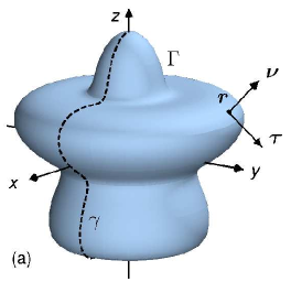
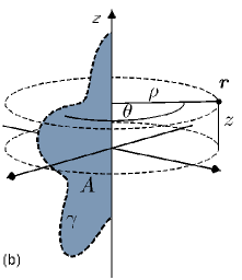
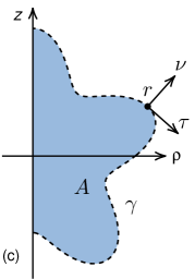
Figure 1: An axially symmetric surface $\Gamma$ generated by a curve $\gamma$. (a) A point ${{\boldsymbol{r}}}$ on $\Gamma$ has outward unit normal $\boldsymbol{\nu}$ and tangent vector $\boldsymbol{\tau}$. (b) ${{\boldsymbol{r}}}$ has radial distance $\rho$, azimuthal angle $\theta$, and height $z$. The two-dimensional domain $A$ is bounded by $\gamma$ and the $z$-axis. (c) Coordinate axes and vectors in the half-plane $\theta=0$.

2 Notation and integral equation

Let $\Gamma$ be an axially symmetric surface enclosing a three-dimensional domain $V$ (a body of revolution) and let

$${{\boldsymbol{r}}}=(x,y,z)=(\rho\cos{\theta},\rho\sin{\theta},z)$$

denote points in $\mathbb{R}^{3}$. Here $\rho=\sqrt{x^{2}+y^{2}}$ is the radial distance from ${{\boldsymbol{r}}}$ to the $z$-axis and $\theta$ is the azimuthal angle. The outward unit normal vector at a point ${{\boldsymbol{r}}}$ on $\Gamma$ is $\boldsymbol{\nu}=(\nu_{\rho}\cos{\theta},\nu_{\rho}\sin{\theta},\nu_{z})$ and $\boldsymbol{\tau}=(\nu_{z}\cos{\theta},\nu_{z}\sin{\theta},-\nu_{\rho})$ is a unit tangent vector. See Figure 1(a) and 1(b).

The angle $\theta=0$ defines a half-plane in $\mathbb{R}^{3}$ whose intersection with $\Gamma$ corresponds to a generating curve $\gamma$. We introduce $r=(\rho,z)$ for points in this half-plane and let $A$ be the two-dimensional closed region bounded by $\gamma$ and the $z$-axis. The outward unit normal at a point $r$ on $\gamma$ is $\nu=(\nu_{\rho},\nu_{z})$ and $\tau=(\nu_{z},-\nu_{\rho})$ is a tangent. See Figure 1(c).

We shall discretize the three layer potential operators $S$, $K_{\boldsymbol{\nu}}$, and $K_{\boldsymbol{\tau}}$ defined by their actions on a layer density $\varrho$ on $\Gamma$ as

$$S\varrho({{\boldsymbol{r}}}) =\int_{\Gamma}\frac{e^{{\rm i}k|{{\boldsymbol{r}}}-{{\boldsymbol{r}}}^{\prime}|}}{4\pi|{{\boldsymbol{r}}}-{{\boldsymbol{r}}}^{\prime}|}\varrho({{\boldsymbol{r}}}^{\prime})\,{\rm d}\Gamma^{\prime}\,,$$ (1)

$$K_{\boldsymbol{\nu}}\varrho({{\boldsymbol{r}}}) =\int_{\Gamma}\frac{\partial}{\partial\boldsymbol{\nu}}\frac{e^{{\rm i}k|{{\boldsymbol{r}}}-{{\boldsymbol{r}}}^{\prime}|}}{4\pi|{{\boldsymbol{r}}}-{{\boldsymbol{r}}}^{\prime}|}\varrho({{\boldsymbol{r}}}^{\prime})\,{\rm d}\Gamma^{\prime}\,,$$ (2)

$$K_{\boldsymbol{\tau}}\varrho({{\boldsymbol{r}}}) =\int_{\Gamma}\frac{\partial}{\partial\boldsymbol{\tau}}\frac{e^{{\rm i}k|{{\boldsymbol{r}}}-{{\boldsymbol{r}}}^{\prime}|}}{4\pi|{{\boldsymbol{r}}}-{{\boldsymbol{r}}}^{\prime}|}\varrho({{\boldsymbol{r}}}^{\prime})\,{\rm d}\Gamma^{\prime}\,.$$ (3)

Here $k$ is the wavenumber and differentiation with respect to $\boldsymbol{\nu}$ and to $\boldsymbol{\tau}$ denote normal- and tangential derivatives. The representation

$$u({{\boldsymbol{r}}})=S\varrho({{\boldsymbol{r}}})\,,\quad{{\boldsymbol{r}}}\in V\cup\Gamma\,,$$ (4)

for a solution $u({{\boldsymbol{r}}})$ to the interior Neumann problem for the Helmholtz equation with boundary condition $f({{\boldsymbol{r}}})$ on $\Gamma$

$$\Delta u({{\boldsymbol{r}}})+k^{2}u({{\boldsymbol{r}}})=0\,,\quad{{\boldsymbol{r}}}\in V\,,$$ (5)

$$\boldsymbol{\nu}\cdot\nabla u({{\boldsymbol{r}}})=f({{\boldsymbol{r}}})\,,\quad{{\boldsymbol{r}}}\in\Gamma\,,$$ (6)

gives the integral equation

$$\left(I+2K_{\boldsymbol{\nu}}\right)\varrho({{\boldsymbol{r}}})=2f({{\boldsymbol{r}}})\,,\quad{{\boldsymbol{r}}}\in\Gamma\,.$$ (7)

In order to normalize solutions $u^{\rm h}({{\boldsymbol{r}}})$ to (5) and (6) with homogeneous boundary conditions we use

$$\int_{V}\left|u^{\rm h}({{\boldsymbol{r}}})\right|^{2}\,{\rm d}V=\frac{1}{2k^{2}}\int_{\Gamma}({{\boldsymbol{r}}}\cdot\boldsymbol{\nu})\left(k^{2}\left|u^{\rm h}({{\boldsymbol{r}}})\right|^{2}-\left|\nabla u^{\rm h}({{\boldsymbol{r}}})\right|^{2}\right)\,{\rm d}\Gamma\,,$$ (8)

which is a special case of a formula due to Barnett [4, eq. (12)]. See also Barnett and Hassell [6, eq. (47)].

The operators $K_{\boldsymbol{\nu}}$ and $K_{\boldsymbol{\tau}}$ can be discretized in similar ways. In what follows we concentrate on the operators $S$ and $K_{\boldsymbol{\nu}}$. We comment on $K_{\boldsymbol{\tau}}$, needed in (8), only in situations where its discretization differs from that of $K_{\boldsymbol{\nu}}$.

3 Splittings of kernels

The kernels $S({{\boldsymbol{r}}},{{\boldsymbol{r}}}^{\prime})$ and $K_{\boldsymbol{\nu}}({{\boldsymbol{r}}},{{\boldsymbol{r}}}^{\prime})$ of the operators $S$ and $K_{\boldsymbol{\nu}}$ are weakly singular at ${{\boldsymbol{r}}}^{\prime}={{\boldsymbol{r}}}$. These singularities cause problems when azimuthal Fourier coefficients of $S({{\boldsymbol{r}}},{{\boldsymbol{r}}}^{\prime})$ and $K_{\boldsymbol{\nu}}({{\boldsymbol{r}}},{{\boldsymbol{r}}}^{\prime})$, also called modal Green’s functions or transformed kernels, are to be evaluated numerically. In this paper we split $S({{\boldsymbol{r}}},{{\boldsymbol{r}}}^{\prime})$ and $K_{\boldsymbol{\nu}}({{\boldsymbol{r}}},{{\boldsymbol{r}}}^{\prime})$ as

$$S({{\boldsymbol{r}}},{{\boldsymbol{r}}}^{\prime}) =Z({{\boldsymbol{r}}},{{\boldsymbol{r}}}^{\prime})\left(H_{1}({{\boldsymbol{r}}},{{\boldsymbol{r}}}^{\prime})+{\rm i}H_{2}({{\boldsymbol{r}}},{{\boldsymbol{r}}}^{\prime})\right)\,,$$ (9)

$$K_{\boldsymbol{\nu}}({{\boldsymbol{r}}},{{\boldsymbol{r}}}^{\prime}) =D_{\boldsymbol{\nu}}({{\boldsymbol{r}}},{{\boldsymbol{r}}}^{\prime})\left(H_{3}({{\boldsymbol{r}}},{{\boldsymbol{r}}}^{\prime})+{\rm i}H_{4}({{\boldsymbol{r}}},{{\boldsymbol{r}}}^{\prime})\right)\,,$$ (10)

where

$$Z({{\boldsymbol{r}}},{{\boldsymbol{r}}}^{\prime}) =\frac{1}{4\pi|{{\boldsymbol{r}}}-{{\boldsymbol{r}}}^{\prime}|}\,,$$ (11)

$$D_{\boldsymbol{\nu}}({{\boldsymbol{r}}},{{\boldsymbol{r}}}^{\prime}) =-\frac{\nu_{\rho}(\rho-\rho^{\prime}\cos(\theta-\theta^{\prime}))+\nu_{z}(z-z^{\prime})}{4\pi|{{\boldsymbol{r}}}-{{\boldsymbol{r}}}^{\prime}|^{3}}\,,$$ (12)

$$H_{1}({{\boldsymbol{r}}},{{\boldsymbol{r}}}^{\prime}) =\cos(k|{{\boldsymbol{r}}}-{{\boldsymbol{r}}}^{\prime}|)\,,$$ (13)

$$H_{2}({{\boldsymbol{r}}},{{\boldsymbol{r}}}^{\prime}) =\sin(k|{{\boldsymbol{r}}}-{{\boldsymbol{r}}}^{\prime}|)\,,$$ (14)

$$H_{3}({{\boldsymbol{r}}},{{\boldsymbol{r}}}^{\prime}) =\cos(k|{{\boldsymbol{r}}}-{{\boldsymbol{r}}}^{\prime}|)+k|{{\boldsymbol{r}}}-{{\boldsymbol{r}}}^{\prime}|\sin(k|{{\boldsymbol{r}}}-{{\boldsymbol{r}}}^{\prime}|)\,,$$ (15)

$$H_{4}({{\boldsymbol{r}}},{{\boldsymbol{r}}}^{\prime}) =\sin(k|{{\boldsymbol{r}}}-{{\boldsymbol{r}}}^{\prime}|)-k|{{\boldsymbol{r}}}-{{\boldsymbol{r}}}^{\prime}|\cos(k|{{\boldsymbol{r}}}-{{\boldsymbol{r}}}^{\prime}|)\,,$$ (16)

and

$$|{{\boldsymbol{r}}}-{{\boldsymbol{r}}}^{\prime}|=\sqrt{\rho^{2}+\rho^{\prime 2}-2\rho\rho^{\prime}\cos(\theta-\theta^{\prime})+(z-z^{\prime})^{2}}\,.$$ (17)

Splittings such as (9) and (10) can facilitate the evaluation of modal Green’s functions, as pointed out in [10]. See [28, Section II] for a review of other splitting options for $S({{\boldsymbol{r}}},{{\boldsymbol{r}}}^{\prime})$ and [14] for efficient splitting-free modal Green’s function evaluation techniques.

4 Fourier series expansions

The first step in our discretization scheme for  (4) and (7) is an azimuthal Fourier transformation. For this, several $2\pi$-periodic quantities need to be expanded in Fourier series. We define the azimuthal Fourier coefficients

$$g_{n}(r) =\frac{1}{\sqrt{2\pi}}\int_{-\pi}^{\pi}e^{-{\rm i}n\theta}g({{\boldsymbol{r}}})\,{\rm d}\theta\,,\quad g=f,\varrho,u\,,$$ (18)

$$G_{n}(r,r^{\prime}) =\frac{1}{\sqrt{2\pi}}\int_{-\pi}^{\pi}e^{-{\rm i}n(\theta-\theta^{\prime})}G({{\boldsymbol{r}}},{{\boldsymbol{r}}}^{\prime})\,{\rm d}(\theta-\theta^{\prime})\,,$$ (19)

where $G$ can represent any of the functions $D_{\boldsymbol{\nu}}$, $D_{\boldsymbol{\nu}}H_{3}$, $D_{\boldsymbol{\nu}}H_{4}$, $H_{1}$, $H_{3}$, $K_{\boldsymbol{\nu}}$, $D_{\boldsymbol{\tau}}$, $K_{\boldsymbol{\tau}}$, $S$, $Z$, $ZH_{1}$, and $ZH_{2}$. The subscript $n$ is called the azimuthal index.

Expansion and integration over $\theta^{\prime}$ gives for (4) and (7)

$$u_{n}(r)=\sqrt{2\pi}\int_{\gamma}S_{n}(r,r^{\prime})\varrho_{n}(r^{\prime})\rho^{\prime}\,{\rm d}\gamma^{\prime}\,,\quad r\in A\,,$$ (20)

$$\varrho_{n}(r)+2\sqrt{2\pi}\int_{\gamma}K_{\nu n}(r,r^{\prime})\varrho_{n}(r^{\prime})\rho^{\prime}\,{\rm d}\gamma^{\prime}=2f_{n}(r)\,,\quad r\in\gamma\,.$$ (21)

Solving the full integral equation (7) and evaluating the field $u({{\boldsymbol{r}}})$ of (4) amounts to solving a series of modal integral equations (21) for $\varrho_{n}$, $n=0,\pm 1,\pm 2,\ldots$, and then retrieving $u({{\boldsymbol{r}}})$ by summation of its Fourier series. In this paper, since we are chiefly interested in Neumann Laplace eigenfunctions, we concentrate on solving (21) and on evaluating $u_{n}(r)$ of (20) for individual modes $n$. Note that a solution $\varrho_{n}(r)$ to (21) corresponds to a modal field $u_{n}(r)$ whenever $f_{n}(r)$ is non-zero. The $j$th homogeneous solution $\varrho_{n,j}(r)$ to (21) corresponds to a modal eigenfunction $u_{n,j}(r)$ such that

$$u_{n,j}({{\boldsymbol{r}}})=\frac{1}{\sqrt{2\pi}}u_{n,j}(r)e^{in\theta}$$ (22)

is a Neumann Laplace eigenfunction of the original Helmholtz problem (5) and (6). Then $k^{2}$ is a Neumann Laplace eigenvalue and $k$ is a Neumann eigenwavenumber $k_{n,j}$.

Expansion for (8) with $u^{\rm h}_{n}(r)=u_{n,j}(r)$ gives

$$\int_{A}\left|u_{n,j}(r)\right|^{2}\rho\,{\rm d}A=\\ \frac{1}{2k_{n,j}^{2}}\int_{\gamma}(r\cdot\nu)\left(\left(k_{n,j}^{2}-\frac{n^{2}}{\rho^{2}}\right)\left|u_{n,j}(r)\right|^{2}-\left|\tau\cdot\nabla u_{n,j}(r)\right|^{2}\right)\rho\,{\rm d}\gamma\,.$$ (23)

Modal eigenfunctions, normalized with respect to this energy integral, are needed in the evaluation of resonances exited by sources, in the comparison of field strengths for different eigenfunctions, and in convergence tests [21, Chapter 5].

The Fourier coefficients of a product of two $2\pi$-periodic functions $g({{\boldsymbol{r}}})$ and $h({{\boldsymbol{r}}})$ with coefficients $g_{n}(r)$ and $h_{n}(r)$ can be obtained by convolution

$$(gh)_{n}(r)=\frac{1}{\sqrt{2\pi}}\sum_{m=-\infty}^{\infty}g_{m}(r)h_{n-m}(r)\,.$$ (24)

5 Discretization – overview I

We seek, for a given $n$, a Nyström discretization of (20) and of (21). There are two difficulties here: First, the logarithmically singular kernels $S_{n}(r,r^{\prime})$ and $K_{\nu n}(r,r^{\prime})$ need to be evaluated at a set of point-pairs $(r,r^{\prime})$. Second, suitable quadrature weights need to be found for integration along $\gamma$.

When $r$ and $r^{\prime}$ are distant, the kernels $S_{n}(r,r^{\prime})$ and $K_{\nu n}(r,r^{\prime})$ are evaluated from their definitions (19) using discrete Fourier transform techniques (FFT) in the azimuthal direction.

When $r$ and $r^{\prime}$ are close, we split $S_{n}(r,r^{\prime})$ and $K_{\nu n}(r,r^{\prime})$ into two parts each: One part which again is computed directly via FFT and another part which is computed using convolution of $Z_{n}(r,r^{\prime})$ with $H_{1n}(r,r^{\prime})$ and of $D_{\nu n}(r,r^{\prime})$ with $H_{3n}(r,r^{\prime})$, respectively. These splittings, originating from (9) and (10), are further discussed in Section 6.

The functions $H_{1n}(r,r^{\prime})$ and $H_{3n}(r,r^{\prime})$, needed for the convolution, are computed via FFT. The functions $Z_{n}(r,r^{\prime})$ and $D_{\nu n}(r,r^{\prime})$, also needed for the convolution, are treated using semi-analytical techniques described in Section 7.

The construction of quadrature weights which capture the logarithmic singularities of $S_{n}(r,r^{\prime})$ and $K_{\nu n}(r,r^{\prime})$, assuming that $\varrho_{n}(r)$ is smooth, is described in Sections 9 and 10.

For simplicity, all FFT operations are controlled by a single integer $N$. When doing a Fourier series expansion of a function, $g({{\boldsymbol{r}}})$ say, as to get coefficients

$$g_{n}(r)=\frac{1}{\sqrt{2\pi}}\int_{-\pi}^{\pi}e^{-{\rm i}n\theta}g({{\boldsymbol{r}}})\,{\rm d}\theta\,,$$ (25)

we use $2N+1$ equispaced points in the azimuthal direction so that

$$g_{n}(r)\approx\frac{\sqrt{2\pi}}{2N+1}\sum_{m=-N}^{N}e^{-{\rm i}n\theta_{m}}g(\rho\cos{\theta_{m}},\rho\sin{\theta_{m}},z)\,,\qquad\theta_{m}=\frac{2\pi m}{2N+1}\,.$$ (26)

We note, but do not exploit, that the need for azimuthal resolution of $g({{\boldsymbol{r}}})$ may vary with $z$.

A convolution, such as (24), is truncated to

$$(gh)_{n}(r)=\frac{1}{\sqrt{2\pi}}\sum_{m=\max\{n-N,-N\}}^{\min\{N,N+n\}}g_{m}(r)h_{n-m}(r)\,.$$ (27)

We note, but do not exploit, that other limits in the sum of (27) can be more efficient in certain situations.

6 The transformed kernels $S_{n}(r,r^{\prime})$ and $K_{\nu n}(r,r^{\prime})$

The kernels $S_{n}(r,r^{\prime})$ and $K_{\nu n}(r,r^{\prime})$ of (19), appearing in (20) and (21), can be split using (9) and (10) as

$$S_{n}(r,r^{\prime})=\frac{1}{\sqrt{2\pi}}\int_{-\pi}^{\pi}e^{-{\rm i}n(\theta-\theta^{\prime})}Z({{\boldsymbol{r}}},{{\boldsymbol{r}}}^{\prime})H_{1}({{\boldsymbol{r}}},{{\boldsymbol{r}}}^{\prime})\,{\rm d}(\theta-\theta^{\prime})\\ +\frac{{\rm i}}{\sqrt{2\pi}}\int_{-\pi}^{\pi}e^{-{\rm i}n(\theta-\theta^{\prime})}Z({{\boldsymbol{r}}},{{\boldsymbol{r}}}^{\prime})H_{2}({{\boldsymbol{r}}},{{\boldsymbol{r}}}^{\prime})\,{\rm d}(\theta-\theta^{\prime})$$ (28)

and

$$K_{\nu n}(r,r^{\prime})=\frac{1}{\sqrt{2\pi}}\int_{-\pi}^{\pi}e^{-{\rm i}n(\theta-\theta^{\prime})}D_{\boldsymbol{\nu}}({{\boldsymbol{r}}},{{\boldsymbol{r}}}^{\prime})H_{3}({{\boldsymbol{r}}},{{\boldsymbol{r}}}^{\prime})\,{\rm d}(\theta-\theta^{\prime})\\ +\frac{{\rm i}}{\sqrt{2\pi}}\int_{-\pi}^{\pi}e^{-{\rm i}n(\theta-\theta^{\prime})}D_{\boldsymbol{\nu}}({{\boldsymbol{r}}},{{\boldsymbol{r}}}^{\prime})H_{4}({{\boldsymbol{r}}},{{\boldsymbol{r}}}^{\prime})\,{\rm d}(\theta-\theta^{\prime})\,.$$ (29)

These splittings are useful when $r$ and $r^{\prime}$ are close. Then, the second integrals in (28) and (29) have smooth integrands and are computed via FFT, or using straight-forward integration if only a single $n$ is of interest. The first integrals in (28) and (29) have non-smooth integrands and are computed via convolution of $Z_{n}(r,r^{\prime})$ with $H_{1n}(r,r^{\prime})$ and of $D_{\nu n}(r,r^{\prime})$ with $H_{3n}(r,r^{\prime})$.

We now explain the benefit of this strategy more in detail. For $r$ and $r^{\prime}$ close, the functions $D_{\boldsymbol{\nu}}H_{4}$, $H_{1}$, $H_{3}$, $ZH_{2}$ are smooth while $D_{\boldsymbol{\nu}}$, $D_{\boldsymbol{\nu}}H_{3}$, $H_{2}$, $H_{4}$, $Z$, $ZH_{1}$ are non-smooth. The Fourier coefficients $g_{n}(r)$ of a smooth function $g({{\boldsymbol{r}}})$ decay rapidly with $n$ and the individual coefficients $g_{n}(r)$ converge rapidly with $N$ in the FFT. An individual coefficient $(gh)_{n}(r)$ in the convolution (27) of two series of coefficients $g_{m}(r)$ and $h_{m}(r)$ has a rapid asymptotic convergence with $N$ if at least one series has rapidly decaying coefficients – compare the discussion of product integration in [15, Section 6.1]. If, for $r$ and $r^{\prime}$ close, no splitting was used and the second integrals in (28) and (29) were to be computed via convolution along with the first integrals, as in [31], then two slowly decaying series would be convolved and slower convergence in the azimuthal direction is expected. In other words, the functions $(ZH_{1})_{n}(r,r^{\prime})$ and $(D_{\boldsymbol{\nu}}H_{3})_{n}(r,r^{\prime})$ converge rapidly with $N$ if computed via convolution (given that $Z_{n}(r,r^{\prime})$ and $D_{\nu n}(r,r^{\prime})$ are available), but slowly if computed via FFT. The functions $(ZH_{2})_{n}(r,r^{\prime})$ and $(D_{\boldsymbol{\nu}}H_{4})_{n}(r,r^{\prime})$ converge rapidly with $N$ if computed via FFT, but slowly if computed via convolution.

A precise definition of what it means that $r$ and $r^{\prime}$ are close is given in Section 12.1.

7 The functions $Z_{n}(r,r^{\prime})$ and $D_{\nu n}(r,r^{\prime})$

The functions $Z_{n}(r,r^{\prime})$ and $D_{\nu n}(r,r^{\prime})$ of (19), needed for the convolution of the first integrals in (28) and (29) when $r$ and $r^{\prime}$ are close, are evaluated using semi-analytical techniques and special functions. There are several ways to proceed. One option is presented in [28, Section III]. We follow Refs. [8, 31] and write

$$Z_{n}(r,r^{\prime})=\frac{1}{\sqrt{8\pi^{3}\rho\rho^{\prime}}}\mathfrak{Q}_{n-\frac{1}{2}}(\chi)$$ (30)

and

$$D_{\nu n}(r,r^{\prime})=\frac{1}{\sqrt{8\pi^{3}\rho\rho^{\prime}}}\left[\left(d_{\nu}(r,r^{\prime})-\frac{\nu_{\rho}}{2\rho}\right)\mathfrak{R}_{n}(\chi)-\frac{\nu_{\rho}}{2\rho}\mathfrak{Q}_{n-\frac{1}{2}}(\chi)\right]\,.$$ (31)

Here

$$\chi=1+\frac{|r-r^{\prime}|^{2}}{2\rho\rho^{\prime}}\,,$$ (32)

$$d_{\nu}(r,r^{\prime})=\frac{\nu\cdot(r-r^{\prime})}{|r-r^{\prime}|^{2}}\,,$$ (33)

$$\mathfrak{R}_{n}(\chi)=\frac{2n-1}{\chi+1}\left(\chi\mathfrak{Q}_{n-\frac{1}{2}}(\chi)-\mathfrak{Q}_{n-\frac{3}{2}}(\chi)\right)\,,\qquad n\geq 0\,,$$ (34)

and $\mathfrak{Q}_{n-\frac{1}{2}}(\chi)$ are half-integer degree Legendre functions of the second kind whose evaluation is discussed in Section 8. Note that $\chi\geq 1$.

8 The evaluation of $\mathfrak{Q}_{n-\frac{1}{2}}(\chi)$ and $\mathfrak{R}_{n}(\chi)$

The Legendre functions $\mathfrak{Q}_{n-\frac{1}{2}}(\chi)$, which for $\chi\geq 1$ may be called toroidal harmonics, have logarithmic singularities at $\chi=1$ but are otherwise analytic. We only need to consider non-negative integers $n$ since it holds that $\mathfrak{Q}_{-n-\frac{1}{2}}(\chi)=\mathfrak{Q}_{n-\frac{1}{2}}(\chi)$. The behavior at infinity is [1, eq. (8.1.3)]

$$\lim_{\chi\to\infty}\mathfrak{Q}_{n-\frac{1}{2}}(\chi)\propto\chi^{-n-\frac{1}{2}}\,,\qquad n\geq 0\,.$$ (35)

The functions $\mathfrak{Q}_{n-\frac{1}{2}}(\chi)$ can be evaluated in several ways. We rely on two methods: forward recursion and backward recursion. The forward recursion is cheap, but unstable for all $\chi>1$ and sufficiently high $n$. The backward recursion is stable, but more expensive. It is particularly expensive for $\chi$ close to unity.

The forward recursion reads [1, eq. (8.5.3)]

$$\mathfrak{Q}_{n-\frac{1}{2}}(\chi)=\frac{4n-4}{2n-1}\chi\mathfrak{Q}_{n-\frac{3}{2}}(\chi)-\frac{2n-3}{2n-1}\mathfrak{Q}_{n-\frac{5}{2}}(\chi)\,,\qquad n=2,\ldots,N\,,$$ (36)

and is, for $\chi>1$, initiated by [1, eqs. (8.13.3) and (8.13.7)]

$$\mathfrak{Q}_{-\frac{1}{2}}(\chi) =\sqrt{\frac{2}{\chi+1}}K_{\rm cei}\left(\frac{2}{\chi+1}\right)\,,$$ (37)

$$\mathfrak{Q}_{\frac{1}{2}}(\chi) =\chi\sqrt{\frac{2}{\chi+1}}K_{\rm cei}\left(\frac{2}{\chi+1}\right)-\sqrt{2(\chi+1)}E_{\rm cei}\left(\frac{2}{\chi+1}\right)\,,$$ (38)

where $K_{\rm cei}(m)$ and $E_{\rm cei}(m)$ are complete elliptic integrals of the first and second kind, respectively, defined as

$$K_{\rm cei}(m) =\int_{0}^{\pi/2}\frac{\,{\rm d}\theta}{\sqrt{1-m\sin^{2}\theta}}\,,$$ (39)

$$E_{\rm cei}(m) =\int_{0}^{\pi/2}\sqrt{1-m\sin^{2}\theta}\;{\rm d}\theta\,,$$ (40)

Note that the definitions of complete elliptic integrals in [1] differ between different sections.

The backward recursion is the forward recursion run backwards. It starts at step $n=M$ with two randomly chosen values for $\mathfrak{Q}_{M+\frac{1}{2}}(\chi)$ and $\mathfrak{Q}_{M+\frac{3}{2}}(\chi)$ and is run down to $n=0$. Then all function values are normalized so that $\mathfrak{Q}_{-\frac{1}{2}}(\chi)$ agrees with (37). Given that (37) is accurate to some precision, the values of $\mathfrak{Q}_{n-\frac{1}{2}}(\chi)$, $n=1,\ldots,N$, have that same accuracy when $M\gg N$ is sufficiently large. The minimal value of $M$ which has this property depends on $\chi$ and on $N$, see [13, Section 4.6.1]. Alternatively, for $\chi$ close to unity, the backward recursion could start at step $n=N$ with $\mathfrak{Q}_{N-\frac{1}{2}}(\chi)$ computed according to [32]. See [1, Section 8.15] for a similar suggestion and [12] and [13, Section 12.3] for even more options.

In the numerical examples of Section 13 we choose backward recursion with $M=N+80$ for $\chi\geq 1.008$ and forward recursion for $1<\chi<1.008$. To evaluate (37) and (38) we use the Matlab function ellipke, modified as to give better precision when $\chi$ is close to unity and $\chi-1$ is known to higher absolute accuracy than $\chi$ itself, compare (32).

The functions $\mathfrak{R}_{n}(\chi)$ are slightly better behaved than $\mathfrak{Q}_{n-\frac{1}{2}}(\chi)$ since they are finite at $\chi=1$. Their values are obtained most easily through their definition (34) in terms of $\mathfrak{Q}_{n-\frac{1}{2}}(\chi)$. One can also use the recursion

$$\mathfrak{R}_{n}(\chi)=\frac{4n-4}{2n-3}\chi\mathfrak{R}_{n-1}(\chi)-\frac{2n-1}{2n-3}\mathfrak{R}_{n-2}(\chi)\,,\qquad n=2,\ldots,N\,,$$ (41)

initiated by

$$\mathfrak{R}_{0}(\chi) =-\sqrt{\frac{2}{\chi+1}}E_{\rm cei}\left(\frac{2}{\chi+1}\right)\,,$$ (42)

$$\mathfrak{R}_{1}(\chi) =\sqrt{\frac{2}{\chi+1}}\left((\chi-1)K_{\rm cei}\left(\frac{2}{\chi+1}\right)-\chi E_{\rm cei}\left(\frac{2}{\chi+1}\right)\right)\,.$$ (43)

9 Product integration for singular integrals

This section summarizes and extends a high-order accurate panel-based analytic product integration scheme applicable to integrals whose kernels contain logarithmic- and Cauchy-type singularities. The scheme was first presented in [16] and later adapted to the Nyström discretization of singular integral operators of planar scattering theory in [17, 19]. In the present work, the scheme is used for discretization along $\gamma$ of operators containing the functions $\mathfrak{Q}_{n-\frac{1}{2}}(\chi)$ and $d_{\tau}(r,r^{\prime})$, as explained in Sections 10, 11, and 12. Functions with logarithmic singularities occur in $Z_{n}(r,r^{\prime})$ for $r\in A$ and in $D_{\nu n}(r,r^{\prime})$ for $r\in\gamma$. The sum of functions with logarithmic- and Cauchy-type singularities occurs in $D_{\tau n}(r,r^{\prime})$.

Consider first the discretization of an integral

$$I_{p}(r)=\int_{\gamma_{p}}G(r,r^{\prime})\varrho(r^{\prime})\,{\rm d}\gamma^{\prime}\,,$$ (44)

where $G(r,r^{\prime})$ is a smooth kernel, $\varrho(r)$ is a smooth layer density, $\gamma_{p}$ is a quadrature panel on a curve $\gamma$, and $r$ is a point close to, or on, $\gamma_{p}$. Let $r(t)=(\rho(t),z(t))$ be a parameterization of $\gamma$. Using $n_{\rm pt}$-point Gauss–Legendre quadrature with nodes and weights $t_{j}$ and $w_{j}$, $j=1,\ldots,n_{\rm pt}$, on $\gamma_{p}$ it holds to high accuracy

$$I_{p}(r)=\sum_{j}G(r,r_{j})\varrho_{j}s_{j}w_{j}\,.$$ (45)

Here $r_{j}=r(t_{j})$, $\varrho_{j}=\varrho(r(t_{j}))$, and $s_{j}=|{\rm d}r(t_{j})/{\rm d}t|$. When we discretize (20) and (21) we shall use a Nyström scheme based on panelwise discretization.

We now proceed to find efficient discretizations for (44) when $G(r,r^{\prime})$ is not smooth, but can be split and factorized into smooth parts and parts with known singularities.

9.1 Logarithmic singularity plus smooth part

Consider (44) when $G(r,r^{\prime})$ can be expressed as

$$G(r,r^{\prime})=\log|r-r^{\prime}|G^{(1)}(r,r^{\prime})+G^{(0)}(r,r^{\prime})\,,$$ (46)

where both $G^{(0)}(r,r^{\prime})$ and $G^{(1)}(r,r^{\prime})$ are smooth functions. Then it holds to high accuracy

$$I_{p}(r)=\sum_{j}G^{(0)}(r,r_{j})\varrho_{j}s_{j}w_{j}+\sum_{j}G^{(1)}(r,r_{j})\varrho_{j}s_{j}w_{{\rm L}j}(r)\,,$$ (47)

where $w_{{\rm L}j}(r)$ are $(n_{\rm pt}-1)$th degree product integration weights for the logarithmic kernel in (46). The weights $w_{{\rm L}j}(r)$ can be constructed using the analytic method in [16, Section 2.3].

Adding and subtracting

$$\sum_{j}\log|r-r_{j}|G^{(1)}(r,r_{j})\varrho_{j}s_{j}w_{j}$$

to the right in (47), assuming $r\neq r_{j}$, and using (46) we get the expression

$$I_{p}(r)=\sum_{j}G(r,r_{j})\varrho_{j}s_{j}w_{j}+\sum_{j}G^{(1)}(r,r_{j})\left[\frac{w_{{\rm L}j}(r)}{w_{j}}-\log|r-r_{j}|\right]\varrho_{j}s_{j}w_{j}\,.$$ (48)

Introducing the logarithmic weight corrections $w_{{\rm L}j}^{\rm corr}(r)$ for the terms within square brackets in (48) we arrive at

$$I_{p}(r)=\sum_{j}G(r,r_{j})\varrho_{j}s_{j}w_{j}+\sum_{j}G^{(1)}(r,r_{j})\varrho_{j}s_{j}w_{j}w_{{\rm L}j}^{\rm corr}(r)\,.$$ (49)

The expression (49) is, from a strictly mathematical viewpoint, merely (47) rearranged in a more appetizing form without explicit reference to $G^{(0)}$. An important advantage of (49) over (47) is, however, related to computations and appears whenever $r$ coincides with a discretization point $r_{i}$ on $\gamma$. Then the expressions for the weight corrections simplify greatly. In fact, $w_{{\rm L}j}^{\rm corr}(r_{i})$, $i\neq j$, only depends on the relative length (in parameter) of the quadrature panels upon which $r_{i}$ and $r_{j}$ are situated and on nodes and weights on a canonical panel. See Appendix A.

For $r=r_{j}$ in (49), neither $G(r_{j},r_{j})$ nor $w_{{\rm L}j}^{\rm corr}(r_{j})$ are defined. We revert to (47) and set $w_{j}w_{{\rm L}j}^{\rm corr}(r_{j})=w_{{\rm L}j}(r_{j})$ and $G(r_{j},r_{j})=G^{(0)}(r_{j},r_{j})$. Apart from that, no explicit knowledge of $G^{(0)}(r,r^{\prime})$ is needed in order to implement (49). It suffices to know $G(r,r^{\prime})$ and $G^{(1)}(r,r^{\prime})$ numerically at a set of points.

Remark: We note, but do not exploit, that if $G^{(1)}(r,r^{\prime})=\mathcal{O}(|r-r^{\prime}|)$ as $r\to r^{\prime}$ one can factor out $|r-r^{\prime}|$ from $G^{(1)}(r,r^{\prime})$ and construct product integration for the kernel $|r-r^{\prime}|\log|r-r^{\prime}|$ rather than for $\log|r-r^{\prime}|$.

9.2 Logarithmic- and Cauchy-type singularities plus smooth part

Now consider (44) when $G(r,r^{\prime})$ can be expressed as

$$G(r,r^{\prime})=\log|r-r^{\prime}|G^{(1)}(r,r^{\prime})+\frac{\mu\cdot(r-r^{\prime})}{|r-r^{\prime}|^{2}}G^{(2)}(r,r^{\prime})+G^{(0)}(r,r^{\prime})\,,$$ (50)

where $G^{(0)}(r,r^{\prime})$, $G^{(1)}(r,r^{\prime})$, and $G^{(2)}(r,r^{\prime})$ are smooth and $\mu$ is a unit vector. If $\mu=\nu$ and $r\in\gamma$, then the second kernel on the right in (50) is smooth and we are back to (46). Otherwise we proceed as in Section 9.1 and observe that it holds to high accuracy

$$I_{p}(r)=\sum_{j}G^{(0)}(r,r_{j})\varrho_{j}s_{j}w_{j}+\sum_{j}G^{(1)}(r,r_{j})\varrho_{j}s_{j}w_{{\rm L}j}(r)\\ +\sum_{j}G^{(2)}(r,r_{j})\varrho_{j}w_{{\rm C}j}(r)\,,$$ (51)

where $w_{{\rm L}j}(r)$ are as in (47) and $w_{{\rm C}j}(r)$ are $(n_{\rm pt}-1)$th degree product integration weights for the Cauchy-type kernel in (50). The weights $w_{{\rm C}j}(r)$ can be constructed using the analytic method in [16, Section 2.1].

Adding and subtracting

$$\sum_{j}\log|r-r_{j}|G^{(1)}(r,r_{j})\varrho_{j}s_{j}w_{j}\quad{\rm and}\quad\sum_{j}\frac{\mu\cdot(r-r_{j})}{|r-r_{j}|^{2}}|G^{(2)}(r,r_{j})\varrho_{j}s_{j}w_{j}$$

to the right in (51), assuming $r\neq r_{j}$, and using (50) we arrive at an expression of the form

$$I_{p}(r)=\sum_{j}G(r,r_{j})\varrho_{j}s_{j}w_{j}+\sum_{j}G^{(1)}(r,r_{j})\varrho_{j}s_{j}w_{j}w_{{\rm L}j}^{\rm corr}(r)\\ +\sum_{j}G^{(2)}(r,r_{j})\varrho_{j}w_{{\rm C}j}^{\rm cmp}(r)\,,$$ (52)

where $w_{{\rm C}j}^{\rm cmp}(r)$ are Cauchy-type singular compensation weights.

The weights $w_{{\rm C}j}^{\rm cmp}(r_{i})$ can, similarly to $w_{{\rm L}j}^{\rm corr}(r_{i})$, be constructed in a particularly economical way. See Appendix B. If $r=r_{j}$ we revert to (51) and set $G(r_{j},r_{j})=G^{(0)}(r_{j},r_{j})$. Apart from that, no explicit knowledge of $G^{(0)}(r,r^{\prime})$ is needed in order to implement (52). It suffices to know $G(r,r^{\prime})$, $G^{(1)}(r,r^{\prime})$, and $G^{(2)}(r,r^{\prime})$ numerically at a set of points.

10 Extracting the singularity of $\mathfrak{Q}_{n-\frac{1}{2}}(\chi)$

The function $\mathfrak{Q}_{n-\frac{1}{2}}(\chi)$ can be split into a logarithmically singular part and a remainder whenever $\chi\in(1,3)$ [32]. The splitting reads

$$\mathfrak{Q}_{n-\frac{1}{2}}(\chi)=-\frac{1}{2}\log\left(\chi-1\right){}_{2}F_{1}\left(-n+\frac{1}{2},n+\frac{1}{2};1;\frac{1-\chi}{2}\right)+R\left(\chi,n\right)\,.$$ (53)

Here $R(\chi,n)$ is smooth, $R(1,n)=\log(2)/2+\psi(1)-\psi(n+1/2)$ where $\psi(x)$ is the digamma function, and ${}_{2}F_{1}(a,b;c;x)$ is the hypergeometric function [1, eq. (15.1.1)]

$${}_{2}F_{1}(a,b;c;x)=\sum_{k=0}^{\infty}\frac{(a)_{k}(b)_{k}}{(c)_{k}}\frac{x^{k}}{k!}\,,\qquad|x|<1\,,$$ (54)

where $(\cdot)_{k}$ is the Pochhammer symbol. See also [24, p. 175] for an alternative expression of $\mathfrak{Q}_{\lambda}(\chi)$ compatible with (53) when $\lambda$ is a half-integer.

10.1 Use of the splitting

The splitting (53) is useful for the discretization of (20) and (21). This is so since the singular nature of the kernels $S_{n}(r,r^{\prime})$ and $K_{\nu n}(r,r^{\prime})$ is contained in $\mathfrak{Q}_{n-\frac{1}{2}}(\chi)$, see (28), (29), (30), and (31), and since (53) expresses $\mathfrak{Q}_{n-\frac{1}{2}}(\chi)$ as a sum of a smooth function and a product of a smooth function and a logarithmic kernel, provided $\chi<3$. In Section 9.1 we reviewed kernel-split product integration techniques for the accurate panel-wise discretization of operators with kernels of this type. Comparing (53) to (46) one can see that the expressions are of the same form with ${}_{2}F_{1}$ corresponding to minus $G^{(1)}$.

Within our overall discretization scheme, the kernels of (20) and (21) are expressed in terms of $\mathfrak{Q}_{n-\frac{1}{2}}(\chi)$ only when $r$ and $r^{\prime}$ are close. We highlight the dependence on $|r-r^{\prime}|$ in $\mathfrak{Q}_{n-\frac{1}{2}}(\chi)$ by rewriting (53), using (32), as

$$\mathfrak{Q}_{n-\frac{1}{2}}(\chi)=-\log\left|r-r^{\prime}\right|{}_{2}F_{1}\left(-n+\frac{1}{2},n+\frac{1}{2};1;-\frac{|r-r^{\prime}|^{2}}{4\rho\rho^{\prime}}\right)+R\left(r,r^{\prime},n\right)\,.$$ (55)

Here $R(r,r^{\prime},n)$ is a new remainder which for $r^{\prime}=r$ assumes the value

$$R(r,r,n)=\log(2\rho)+\psi(1)-\psi\left(n+\frac{1}{2}\right)\,.$$ (56)

From a numerical viewpoint, there are some problems with (55). The function ${}_{2}F_{1}$ may be costly to compute for a large number of point pairs $(r,r^{\prime})$ and indices $n$. Furthermore, even if $r^{\prime}$ close to $r$ often means that $\chi$ is close to unity and that $R$ is smooth, this does not have to be the case when $r$ is close to the endpoints of $\gamma$. For example, the fourth argument of ${}_{2}F_{1}$, and ${}_{2}F_{1}$ itself, may then vary rapidly with $\rho^{\prime}$ along an individual quadrature panel. The requirement $\chi<3$ may even be violated so that (53) is no longer valid. Similar problems occur for large $n$ in combination with too wide panels.

To alleviate some of the problems mentioned we truncate the sum in (54) after four terms and introduce

$${}_{2}\tilde{F}_{1}(a,b;x)=\sum_{k=0}^{3}\frac{(a)_{k}(b)_{k}}{(k!)^{2}}x^{k}\,,$$ (57)

and expand $\rho^{\prime}$ around $\rho$ and truncate that expansion, too, after four terms. The result is

$$\mathfrak{Q}_{n-\frac{1}{2}}(\chi)=-\log\left|r-r^{\prime}\right|{}_{2}\tilde{F}_{1}\left(-n+\frac{1}{2},n+\frac{1}{2};-T(r,r^{\prime})\right)+\tilde{R}\left(r,r^{\prime},n\right)\,,$$ (58)

where

$$T(r,r^{\prime})=\frac{|r-r^{\prime}|^{2}}{4\rho^{2}}\sum_{k=0}^{3}\left(\frac{\rho-\rho^{\prime}}{\rho}\right)^{k}\,.$$ (59)

The new splitting (58) is cheaper to implement than (55) and is slightly better balanced. Note that the new remainder $\tilde{R}(r,r^{\prime},n)$ is only $\mathcal{C}^{5}$-smooth away from the $z$-axis, but that this appears to be sufficient for our numerical purposes. See Section 12.2 for additional techniques used to ensure that the splitting (58) can produce an accurate discretization of integral operators containing $\mathfrak{Q}_{n-\frac{1}{2}}(\chi)$ within our product integration framework.

11 The kernel $K_{\tau n}(r,r^{\prime})$

The treatment of $K_{\tau n}(r,r^{\prime})$ closely follows that of $K_{\nu n}(r,r^{\prime})$, but with $\nu$ replaced by $\tau$. For example, equation (31) becomes

$$D_{\tau n}(r,r^{\prime})=\frac{1}{\sqrt{8\pi^{3}\rho\rho^{\prime}}}\left[d_{\tau}(r,r^{\prime})\mathfrak{R}_{n}(\chi)-\frac{\nu_{z}}{2\rho}\left(\mathfrak{R}_{n}(\chi)+\mathfrak{Q}_{n-\frac{1}{2}}(\chi)\right)\right]\,,$$ (60)

where $d_{\tau}(r,r^{\prime})$ is the Cauchy-type singular kernel

$$d_{\tau}(r,r^{\prime})=\frac{\tau\cdot(r-r^{\prime})}{|r-r^{\prime}|^{2}}\,.$$ (61)

When $\chi$ is close to unity we can, for the purpose of discretization, combine (34) and (58) and write $d_{\tau}(r,r^{\prime})\mathfrak{R}_{n}(\chi)$ in (60) as

$$d_{\tau}(r,r^{\prime})\mathfrak{R}_{n}(\chi)=\log|r-r^{\prime}|G^{(1)}(r,r^{\prime})-d_{\tau}(r,r^{\prime})+G^{(0)}(r,r^{\prime})\,,$$ (62)

where

$$G^{(0)}(r,r^{\prime}) =d_{\tau}(r,r^{\prime})\left(\frac{2n-1}{\chi+1}\left(\chi\tilde{R}(r,r^{\prime},n)-\tilde{R}(r,r^{\prime},n-1)\right)+1\right)\,,$$ (63)

$$\begin{split}G^{(1)}(r,r^{\prime})&=-d_{\tau}(r,r^{\prime})\frac{2n-1}{\chi+1}\left(\chi{}_{2}\tilde{F}_{1}\left(-n+\frac{1}{2},n+\frac{1}{2};-T(r,r^{\prime})\right)\right.\\ &\qquad\qquad\qquad\qquad\quad\left.-{}_{2}\tilde{F}_{1}\left(-n+\frac{3}{2},n-\frac{1}{2};-T(r,r^{\prime})\right)\right)\,.\end{split}$$ (64)

The expression (62) is of the type (50) with $\mu=\tau$ and $G^{(2)}(r,r^{\prime})=-1$. The limits of $G^{(0)}(r,r^{\prime})$ and $G^{(1)}(r,r^{\prime})$ are zero as $r^{\prime}\to r$.

12 Discretization – overview II

Our discretization scheme for (4) and (7) contains a large number of steps and computational techniques. Now that most of these have been reviewed, and for ease of reading, we again summarize the main features of the scheme. We also provide important implementational details.

12.1 Quadrature techniques used

Several quadrature techniques are involved. In the azimuthal direction we either use the composite trapezoidal rule or semi-analytical methods combined with FFT and convolution. In the polar direction, where the Nyström scheme is applied, we either use composite Gauss–Legendre quadrature or kernel-split product integration and 16 discretization points per panel. With $n_{\rm pan}$ panels on $\gamma$ and notation as in Section 9, eq. (21) assumes the general form

$$\varrho_{n}(r_{i})+2\sqrt{2\pi}\sum_{j=1}^{m}K_{\nu n}(r_{i},r_{j})\varrho_{n}(r_{j})\rho_{j}s_{j}w_{ij}=2f_{n}(r_{i})\,,\quad i=1,\ldots,m\,,$$ (65)

where $m=16n_{\rm pan}$, $\rho_{j}=\rho(t_{j})$, $t_{j}$ and $w_{ij}$ are nodes and weights on $\gamma$, and the discretization points play the role of both target points $r_{i}$ and source points $r_{j}$. We say that the $16n_{\rm pan}$ points $r_{i}$ constitute a global grid on $\gamma$.

The mesh of quadrature panels on $\gamma$ is approximately uniform. Discretization points located on the same panel or on neighboring panels are said to be close. Point pairs that are not close are said to be distant. It is the interaction between close point pairs that may require semi-analytical methods, convolution, and product integration. Panelwise discretization for distant point pairs is easy: all kernels are considered smooth and we rely exclusively on the underlying quadrature, that is, the trapezoidal rule and composite Gauss–Legendre quadrature with $n_{\rm pt}=16$ and with weights $w_{ij}$ of (65) independent of $i$. The same philosophy is used in [31].

The discretization (65) is a linear system for $16n_{\rm pan}$ unknown pointwise values of the layer density $\varrho_{n}(r)$. The system matrix can, based on panel affiliation, be partitioned into $n_{\rm pan}\times n_{\rm pan}$ square blocks with 256 entries each. All interaction between close point pairs is contained in the block tridiagonal part of this partitioned matrix.

12.2 The discretization of the integral operator in (21)

Let $B$ denote the partitioned matrix corresponding to the system matrix in (65) and let $B^{(3)}$ denote its block tridiagonal part. All entries of $B$ that lie outside of $B^{(3)}$ are evaluated using underlying quadrature. The same holds for contributions to entries of $B^{(3)}$ that stem from the second integral in (29). Contributions to entries of $B^{(3)}$ that stem from the first integral in (29) are computed via convolution of $D_{\nu n}(r,r^{\prime})$ with $H_{3n}(r,r^{\prime})$. The functions $H_{3n}(r,r^{\prime})$ are computed via FFT. The functions $D_{\nu n}(r,r^{\prime})$ are computed via (31) and the evaluation techniques of Section 8. The quadrature weights associated with $D_{\nu n}(r,r^{\prime})$ are found using the product integration of Section 9.

The discretization of (21) for $r$ and $r^{\prime}$ both close to the endpoints of $\gamma$ poses an extra challenge related to the rapid variation of ${}_{2}\tilde{F}_{1}$ and $\tilde{R}$, see Section 10.1. Therefore we temporarily refine the panels closest to the $z$-axis by binary subdivision $n_{\rm sub}$ times in the direction towards the $z$-axis. Then we discretize on this refined mesh and interpolate the result back to target- and source points on the global grid. This procedure seems to yield fully accurate results with $n_{\rm sub}=9$ for $n_{\rm pt}=16$ and affects entries in the top left $2\times 2$ blocks and bottom right $2\times 2$ blocks of $B^{(3)}$.

High indices $n$, relative to the spacing of points on $\gamma$, also require extra care in the product integration for $\mathfrak{Q}_{n-\frac{1}{2}}(\chi)$. This is so since for large $n$, the splittings of Section 10 are appropriate only in a narrow zone around $\chi=1$. Away from this zone, the functions corresponding to $G^{(0)}$ and $G^{(1)}$ in (46) behave badly (become large, converge slowly when expressed as infinite sums, and suffer from cancellation). The truncation technique of Section 10.1 is not powerful enough to counterbalance this effect on too wide panels. This problem, again, is remedied with temporary refinement. Each quadrature panel is temporarily divided into at most four subpanels with $n_{\rm pt}$ auxiliary discretization points each. The resulting discretization is then interpolated back to the global grid. This procedure affects all entries of $B^{(3)}$. Note that the 10th order accurate Kolm–Rokhlin quadrature of [15, 31] uses at most 24 auxiliary points per panel and per target point for a similar purpose.

The integer $N$, controlling the resolution in the azimuthal direction via (26), is taken to be proportional to $n_{\rm pan}$ with a constant of proportionality depending on the shape of $\gamma$. Note that, for a fixed $N$ and despite all the special techniques used, the cost of computing all entries of $B^{(3)}$ grows only linearly with the number of discretization points on $\gamma$.

12.3 Improved convergence

The quadratures used in (65) have different orders of accuracy. The trapezoidal rule gives exponential convergence in the azimuthal direction; composite Gauss–Legendre quadrature with $n_{\rm pt}=16$ gives 32nd order accuracy for distant interactions in the polar direction; product integration with $n_{\rm pt}=16$ gives 16th order convergence for close interactions.

The convergence of a mixed-quadrature Nyström scheme is controlled by the error in the quadrature with the lowest order. In our scheme, the product integration is the weakest link and it is important to make its error constant small – something which can be achieved by extra resolution of known functions in singular kernels. For example, one can first discretize the parts of (21) that correspond to entries of $B^{(3)}$ using $n_{\rm pt}=32$ with $n_{\rm sub}=11$ and then interpolate the result back to the 16 points per panel on the global grid. See “scheme B” of [18, Section 8.2] for more details. In the numerical examples below we incorporate a simple version of this convergence enhancement technique. The result, typically, is a 30 per cent reduction in the number of global grid points needed to reach a given accuracy in $\varrho_{n}$. The number of kernel evaluations required to form $B^{(3)}$ is, however, increased by a factor of at least four.

12.4 The discretization of other integral operators

The discretization of the integral operator in (20) is, more or less, a subproblem of the discretization of the integral operator in (21). Field evaluations in a post-processor, for $r\notin\gamma$, are particularly simple as $r$ and $r^{\prime}$ never coincide. There is no need to “interpolate back to points on the original panel” and the product integration weights need not be stored after use.

The discretization of operators containing the kernel $K_{\tau n}(r,r^{\prime})$ may seem more involved than the discretization of operators containing $K_{\nu n}(r,r^{\prime})$. The difference being that the product integration now involves (52) for (60) rather than (49) for (31). In practice, the extra complication is minor. The factor corresponding to $G^{(2)}(r,r^{\prime})$ in (52) is a constant, see (62), so the situation is the same as in the two-dimensional examples treated accurately in [19].

13 Numerical examples

Our Fourier–Nyström scheme has been implemented in Matlab. We now test this code for correctness, convergence rate, and achievable accuracy. The numerical examples cover the determination of modal fields, boundary value maps, Neumann eigenwavenumbers, and normalized modal eigenfunctions in the entire computational domain.

Asymptotically, for a body of revolution, the total number of Neumann Laplace eigenfunctions $u_{n,j}({\boldsymbol{r}})$ with eigenwavenumbers $k_{n,j}$ bounded by a value $k_{\rm lim}$ is proportional to $k_{\rm lim}^{3}$. For a given index $n$, the number of modal eigenfunctions $u_{n,j}(r)$ is proportional to $k_{\rm lim}^{2}$. Eigenwavenumbers with $n\neq 0$ are always degenerate since, for example, $k_{n,j}$ and $k_{-n,j}$ are the same with Neumann Laplace eigenfunctions being complex conjugates to each other. For a given $n$, however, and for most bodies of revolution, there is no degeneracy. Our examples use wavenumbers with magnitudes of interest in applications such as mufflers [7] and ultrasound spectroscopy [26], where important wavelengths range from half the diameter of the resonant volume down to a tenth of the diameter. The magnitudes are also comparable to the ones used in other numerical work on axisymmetric Helmholtz problems [31].

The code is executed on a workstation equipped with an Intel Core i7 CPU at 3.20 GHz and 64 GB of memory. We refrain from giving extensive timings since the code is not optimized for execution speed and since the overall complexity is essentially the same as that of the scheme in [31].

13.1 Modal field from external point source in domain with star shaped cross-section

This section tests convergence of the solution to a modal interior Neumann Helmholtz problem (20) and (21) with $n=1$. The body of revolution $V$, shown in Figure 1(a), has a generating curve $\gamma$ parameterized as

$$r(t)=(\rho(t),z(t))=(1+0.25\cos(5t))(\sin(t),\cos(t))\,,\qquad 0\leq t\leq\pi\,.$$ (66)

The boundary condition on $\gamma$ is given by the normal derivative of a field $u_{\rm p}({\boldsymbol{r}})$, excited by a point source at ${{\boldsymbol{r}}}_{\rm p}$ outside $V$

$$u_{\rm p}({\boldsymbol{r}})=5S({{\boldsymbol{r}}},{{\boldsymbol{r}}}_{\rm p})=\frac{5e^{{\rm i}k|{{\boldsymbol{r}}}-{{\boldsymbol{r}}}_{\rm p}|}}{4\pi|{{\boldsymbol{r}}}-{{\boldsymbol{r}}}_{\rm p}|}\,,\qquad k=19,\qquad{{\boldsymbol{r}}}_{\rm p}=(0.5,0,1)\,.$$ (67)

We remark, in connection with (66), that an arc length parameterization is probably more efficient in terms of resolution.

It follows from (67) and the definitions in Sections 2 and 4 that the excited modal fields in $A$ and their derivatives on $\gamma$ are

$$u_{{\rm p}n}(r) =5S_{n}(r,r_{\rm p})\,,\qquad r\in A\,,$$ (68)

$$\nu\cdot\nabla u_{{\rm p}n}(r) =5K_{\nu n}(r,r_{\rm p})\,,\qquad r\in\gamma\,,$$ (69)

$$\tau\cdot\nabla u_{{\rm p}n}(r) =5K_{\tau n}(r,r_{\rm p})\,,\qquad r\in\gamma\,.$$ (70)

The source strength is chosen to be five so that the modulus of the field $u_{{\rm p}1}(r)$ in $V$ peaks approximately at unity. The wavenumber $k=19$ corresponds to about $7.3$ wavelengths across the generalized diameter of $V$.

Our scheme determines the modal field $u_{1}(r)$ by first solving (65) for $\varrho_{1}(r_{i})$ with $f_{1}(r_{i})=5K_{\nu 1}(r_{i},r_{\rm p})$ and then evaluating a discretization of (20). The values of $K_{\nu 1}(r_{i},r_{\rm p})$ are obtained via (19) with $G=K_{\boldsymbol{\nu}}$ and the trapezoidal rule. The mesh is uniformly refined in parameter $t$ (not in arc length) with $n_{\rm pan}$ panels corresponding to $16n_{\rm pan}$ discretization points on $\gamma$. The integer $N$, controlling the resolution in the azimuthal direction, is chosen as $N=4n_{\rm pan}$.

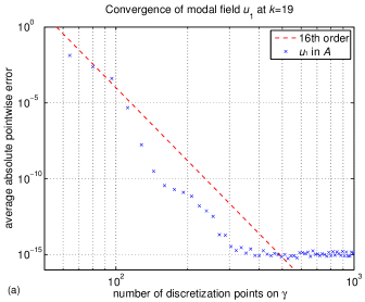
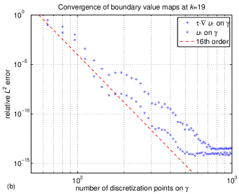
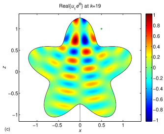
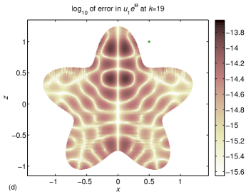
Figure 2: Convergence of the modal field $u_{1}(r)$ excited by a point source of strength 5 located at ${{\boldsymbol{r}}}_{\rm p}=(0.5,0,1)$ and indicated by a green star. The wavenumber is $k=19$. (a) Average absolute pointwise error in $u_{1}(r)$. (b) Relative $L^{2}$ errors in the modal Neumann-to-Dirichlet map $\nu\cdot\nabla u_{1}(r)\mapsto u_{1}(r)$ and in the map $\nu\cdot\nabla u_{1}(r)\mapsto\tau\cdot\nabla u_{1}(r)$. (c) Real part of the field $u_{1}(r)e^{{\rm i}\theta}$ for $\theta=0$ and $\theta=\pi$. (d) $\log_{10}$ of pointwise error in $u_{1}(r)e^{{\rm i}\theta}$ for $\theta=0$ and $\theta=\pi$.

For error estimates we do a comparison with supposedly more accurate reference values derived directly from (67). Figure 2(a) compares our results $u_{1}(r)$ to reference values $u_{{\rm p}1}(r)$, obtained from (68) via (19) with $G=S$ and the trapezoidal rule. The comparison is done under mesh refinement and at 50,276 field points in a cross-section given by the intersection of $V$ and the half-planes $\theta=0$ and $\theta=\pi$. The field points are placed on a uniform $300\times 300$ grid in the square $x\in[-1.2,1.2]$ and $z\in[-1.1,1.3]$. Points outside the cross-section are excluded. Figure 2(a) shows that the convergence is at least 16th order, as expected, and that the achievable average accuracy is around $10\epsilon_{\rm mach}$. The field $u_{1}(r)$ and the distribution of absolute pointwise error are depicted in Figures 2(c) and 2(d). Here the field resolution is increased and 274,800 field points on a uniform $700\times 700$ grid are used. There are 608 discretization point on $\gamma$. It is worth mentioning that even though some field points lie very close to $\gamma$, there is no visible sign of accuracy degradation in the near-surface field evaluation. We get close to machine precision in the entire computational domain – a success which in part can be explained by the low condition number of the system matrix in (65). In this example it is only 114.

Having solved (65) for $\varrho_{1}(r_{i})$, we also evaluate $\tau\cdot\nabla u_{1}(r)$ at the discretization points $r_{i}$ on $\gamma$ and compare with reference values. Our values $\tau\cdot\nabla u_{1}(r_{i})$ are obtained via a discretization of

$$\tau\cdot\nabla u_{n}(r)=\sqrt{2\pi}\int_{\gamma}K_{\tau n}(r,r^{\prime})\varrho_{n}(r^{\prime})\rho^{\prime}\,{\rm d}\gamma^{\prime}\,,\quad r\in\gamma\,,$$ (71)

and the techniques of Section 12.4. The reference values $\tau\cdot\nabla u_{{\rm p}1}(r_{i})$ are obtained from (70) via (19) with $G=K_{\boldsymbol{\tau}}$ and the trapezoidal rule. Accurate computation of $\tau\cdot\nabla u_{n}(r_{i})$ is important whenever (23) is to be used for normalization. Figure 2(b) shows that the achievable $L^{2}$ accuracy in $\tau\cdot\nabla u_{1}(r)$ is roughly the same as that of $u_{1}(r)$ on $\gamma$, albeit somewhat delayed. Had we used numerical differentiation of $u_{1}(r)$ for $\tau\cdot\nabla u_{1}(r)$, rather than the analytical differentiation implicit in (71), precision would have been lost.

As for timings we quote the following: with $640$ global discretization points $r_{i}$ on $\gamma$, and with $2N+1=321$ Fourier coefficients in the convolutions, it takes 65 seconds in total to construct the discretizations of $S_{1}$, $K_{\nu 1}$, and $K_{\tau 1}$, form and solve (65), and compute $u_{1}(r_{i})$ and $\tau\cdot\nabla u_{1}(r_{i})$. Of this time, 30 seconds are spent constructing top left and bottom right blocks of matrices corresponding to discretizations of $Z_{n}$, $D_{\nu n}$, and $D_{\tau n}$, $n=-N,\ldots,N$, using the procedure for near-endpoint evaluation described in Sections 12.2 and 12.3, and 20 seconds are spent on the remaining tridiagonal blocks of these $k$-independent matrices.

13.2 Eigenpair in the unit sphere

This section finds a Neumann eigenwavenumber-eigenfunction pair in the unit sphere. The generating curve $\gamma$ is parameterized by

$$r(t)=(\rho(t),z(t))=(\sin(t),\cos(t))\,,\qquad 0\leq t\leq\pi\,.$$ (72)

Eigenpairs in the sphere can be determined from (5) and (6) with $f({\boldsymbol{r}})=0$ using separation of variables [2, Section 9.3]. Each azimuthal mode $n$ has infinitely many eigenwavenumbers which can be ordered with respect to magnitude by two integers $\ell\geq|n|$ and $m\geq 1$. The number $k_{n,\ell,m}$ is the $m$th positive solution to

$$\frac{{\rm d}j_{\ell}(x)}{{\rm d}x}=0\,,$$ (73)

where $j_{\ell}(x)$ is the spherical Bessel function of order $\ell$.

Our approach is to choose a mode $n$, a mesh on $\gamma$, and an interval $[k_{\rm low},k_{\rm up}]$ where to look for an eigenwavenumber. For simplicity, we use golden section search with the condition number of the system matrix in (65) as the function to be maximized [6, Appendix B]. When a maximum is found, the corresponding $k$ is an approximation of a $k_{n,\ell,m}$. The integers $\ell$ and $m$ are determined by visual inspection of the associated eigenfunction. See [6] for a far more economical way to determine eigenpairs of the Laplacian using integral equation techniques.

Figure 3: Convergence of the Neumann eigenpair $k_{1,1,44}$ and $u_{1,1,44}(r)$ in the unit sphere. The wavenumber $k_{1,1,44}=141.3575204174371$ corresponds to approximately 45 wavelengths across the sphere diameter. x-marks and stars show relative errors as a function of mesh resolution. The error in $u_{1,1,44}(r)$ is measured in $L^{2}$ norm at $\gamma$. Circles show the reciprocal condition number of the system matrix in (65).

The convergence of $k_{1,1,44}$ is shown in Figure 3. Our computed estimates are compared to the correctly rounded value $k_{1,1,44}=141.3575204174371$, obtained via (73). The eigenwavenumbers are densely packed so the interval $[k_{\rm low},k_{\rm up}]$ has to be narrow. We choose $k_{\rm low}=141.34$ and $k_{\rm up}=141.40$. The mesh is uniformly refined with $n_{\rm pan}$ panels corresponding to $16n_{\rm pan}$ discretization points on $\gamma$. The integer $N$, controlling the resolution in the azimuthal direction, is chosen as $N=12n_{\rm pan}$. One can see, in Figure 3, that a condition number of $10^{12}$ and $256$ points on $\gamma$, corresponding to 3.6 points per wavelength along $\gamma$, is sufficient to yield $k_{1,1,44}$ with full machine precision.

Figure 3 also shows convergence of the eigenfunction $u_{1,1,44}(r)$, normalized by $||u_{n,\ell,m}(r)\sqrt{\rho}||_{L^{2}(A)}=1$ and by the requirement that $u_{n,\ell,m}(r)$ is real. A complex constant of unit modulus which rotates the appropriate eigenvector of the system matrix in (65), so that it produces a real valued $u_{n,\ell,m}(r)$ in the directization of (20), is determined with a least squares fit on $\gamma$. Our computed estimates for $u_{1,1,44}(r)$ are compared to reference values obtained from

$$u_{1,1,m}(r(t))=\frac{\sqrt{3}k_{1,1,m}}{\sqrt{2k_{1,1,m}^{2}-4}}\sin(t)\,,\quad r\in\gamma\,.$$ (74)

The relative error is computed in $L^{2}$ norm on $\gamma$. The determination of $u_{1,1,44}(r)$ is a more difficult problem than the determination of $k_{1,1,44}$. Higher resolution is needed for a given relative accuracy and the achievable accuracy is lower.

Even though test problems in the unit sphere often are simple to solve, the problem in this section may be thought of as a little harder. The sphere has 204,646 modal eigenfunctions with $k\leq k_{1,1,44}$ and 2,488 of these are $n=1$ modes. This means that $k=k_{1,1,44}$, corresponding to approximately 45 wavelengths across the sphere diameter, is a rather “high” wavenumber. See the interesting discussion in [6, Section 1] on what wavenumbers are needed in applications and on performance characteristics of different classes of methods used to find them.

13.3 Eigenpairs in domain with star shaped cross-section

This section finds two Neumann eigenwavenumbers and their associated modal eigenfunctions in the body of revolution generated by $\gamma$ of (66). For each azimuthal index $n$ there are infinitely many Neumann eigenwavenumbers. These can be ordered and numbered with respect to their magnitude so that $k_{n,j}$ is the $j$th smallest eigenwavenumber for index $n$. The associated modal eigenfunction $u_{n,j}(r)$ is normalized, as in Section 13.2, by $||u_{n,j}(r)\sqrt{\rho}||_{L^{2}(A)}=1$ and by the requirement that $u_{n,j}(r)$ is real.

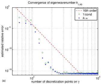
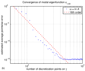
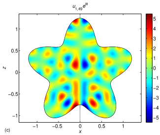
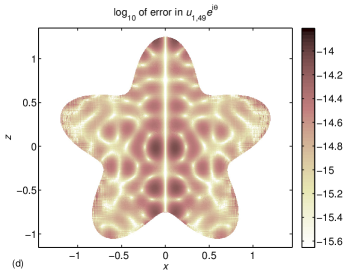
Figure 4: Convergence of the Neumann eigenpair $k_{1,49}$ and $u_{1,49}(r)$. (a) Reciprocal condition number and error in $k_{1,49}$. Reference value $k_{1,49}=19.22942004015467$ is used. (b) Estimated average pointwise error in $u_{1,49}(r)$. (c) The field $u_{1,49}(r)e^{{\rm i}\theta}$ for $\theta=0$ and $\theta=\pi$. (d) $\log_{10}$ of pointwise error in $u_{1,49}(r)e^{{\rm i}\theta}$ for $\theta=0$ and $\theta=\pi$ with $560$ points on $\gamma$.

We first search for $k_{1,49}$ in the interval $k_{\rm low}=19.1$ and $k_{\rm up}=19.3$ using the approach of Section 13.2, but with $N=4n_{\rm pan}$ as in Section 13.1. Figure 4(a) shows convergence under mesh refinement. The eigenwavenumber has converged stably to machine precision with 272 discretization points on $\gamma$, corresponding to an average number of 21.4 points per wavelength along $\gamma$, and we use the converged value $k_{1,49}=19.229420040154672$ as reference value when estimating the error.

Having established $k_{1,49}$, we proceed with a convergence study for the field $u_{1,49}(r)$ in $A$. This investigation is very similar to the study of the modal field $u_{1}(r)$ in Section 13.1. The chief difference being the additional complication of normalizing $u_{1,49}(r)$ using (23). Results are displayed in Figures 4(b), 4(c), and 4(d). Here the pointwise error refers to an estimated absolute pointwise error normalized with the largest value of $|u_{1,49}(r)|$, $r\in A$. The estimated pointwise error at a field point $r$ and with a given number of discretization points on $\gamma$ is taken as the difference between the computed value at $r$ and a better resolved value at $r$, computed with approximately 50 per cent more discretization points on $\gamma$. Figures 4(a) and 4(b) show asymptotic 16th order convergence. The very high achievable accuracy for the normalized modal eigenfunction field, shown in Figures 4(b) and 4(d), is only possible thanks to the accurate implementation of the boundary value maps $\nu\cdot\nabla u_{n}(r)\mapsto u_{n}(r)$ and $\nu\cdot\nabla u_{n}(r)\mapsto\tau\cdot\nabla u_{n}(r)$, tested separately in Figure 2(b) and now used in the discretization of (23).

As an independent test of correctness in the results for $k_{1,49}$ and $u_{1,49}(r)$ we compared our values and fields with those obtained from the finite element 2D axisymmetric solver in COMSOL Multiphysics 4.3b, run on a workstation with 64 GB of memory. With 6,197,297 degrees of freedom in the mesh on $A$, corresponding to 640 degrees of freedom per wavelength, the COMSOL estimates exhibit a relative deviation from our converged result of about $10^{-10}$ in $k_{1,49}$ and of $4\cdot 10^{-8}$ in the maximum value of $|u_{1,49}(r)|$, which for this eigenfunction occurs at $\gamma$. Our scheme needs roughly 11 points per wavelength for that same accuracy, see Figure 4(a) and (b).

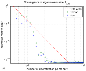
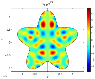
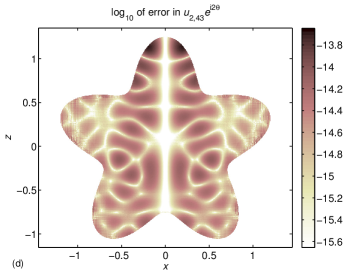
Figure 5: Convergence of the Neumann eigenpair $k_{2,43}$ and $u_{2,43}(r)$. (a) Reciprocal condition number and error in $k_{2,43}$. Reference value $k_{2,43}=19.21873987061249$ is used. (b) Estimated average pointwise error in $u_{2,43}(r)$. (c) The field $u_{2,43}(r)e^{{\rm i}2\theta}$ for $\theta=0$ and $\theta=\pi$. (d) $\log_{10}$ of pointwise error in $u_{2,43}(r)e^{{\rm i}2\theta}$ for $\theta=0$ and $\theta=\pi$ with $560$ points on $\gamma$.

The results of a parallel investigation of the convergence of $k_{2,43}$ and $u_{2,43}(r)$ are shown in Figure 5. The results are very similar to those for $k_{1,49}$ and $u_{1,49}(r)$ and we conclude that computing Neumann eigenpairs is a well conditioned problem at these wavenumbers. With our scheme it is no more difficult, in terms of achievable accuracy, than computing simple modal fields as in Section 13.1.

14 Conclusions and outlook

We have constructed a Fourier–Nyström discretization scheme for second kind Fredholm integral equations with singular kernels in axially symmetric domains and verified it numerically on modal interior Neumann Helmholtz problems. The competitiveness of the scheme lies in high-order convergence, high achievable accuracy, and the ability to evaluate field solutions with uniform accuracy throughout the computational domain. These favorable characteristics are made possible by an explicit kernel-split, panel-based, product integration philosophy which incorporates analytic information about integral kernels to a higher degree than competing methods and allows for on-the-fly computation of nearly singular quadrature rules regardless of where target points are located relative to quadrature panels.

Another advantage of using a Fourier–Nyström scheme, over a full three dimensional PDE eigenvalue solver for axisymmetric problems, is that it enables easier identification and classification of eigenfunctions. One azimuthal index $n$ is treated at a time.

One could argue that the precision offered by our scheme may not be needed in real life applications. In acoustics, sound-hard surfaces with homogeneous Neumann boundary conditions are only coarse models of real surfaces. On the other hand, in electromagnetics there are resonance problems where the mathematical models are very exact. One example is the determination of resonance frequencies and fields in axially symmetric superconducting cavities with ultra-high vacuum and electro-polished surfaces. This problem is important in particle accelerator design [30] and can be modeled as a PDE eigenvalue problem. When the electromagnetic fields are weak enough not to affect the superconductivity, the relative error in the PDE model can be as low as $10^{-12}$, given a generating curve $\gamma$. Furthermore, the superconducting cavities often have corners that subject numerical solvers to much tougher tests than the smooth domains used in the numerical examples of the present paper. Having already developed powerful methods for scattering problems in non-smooth planar domains [17, 19], we intend to generalize our axisymmetric scheme to cope with electromagnetic resonances and non-smooth domains in the near future. The ultimate goal is to include our solvers in a robust particle accelerator simulation package.

Appendix A. The construction of $w_{{\rm L}j}^{\rm corr}(r_{i})$

We first show how to construct the logarithmic weights $w_{{\rm L}j}(r_{i})$ of Section 9.1 which occur in the approximation of

$$I_{p}(r_{i})=\int_{\gamma_{p}}\log|r_{i}-r^{\prime}|G^{(1)}(r_{i},r^{\prime})\varrho(r^{\prime})\,{\rm d}\gamma^{\prime}$$ (A.1)

with an expression of the form

$$I_{p}(r_{i})=\sum_{j}G^{(1)}(r_{i},r_{j})\varrho_{j}s_{j}w_{{\rm L}j}(r_{i})\,.$$ (A.2)

For simplicity we assume that $r_{i}$ and $r_{j}$ are located on the same quadrature panel $\gamma_{p}$ with starting point $r(t_{a})$ and end point $r(t_{b})$. Then the quadrature nodes $t_{j}$ and weights $w_{j}$, corresponding to points $r_{j}$, can be expressed as

$$t_{j}=\frac{t_{b}+t_{a}}{2}+\frac{t_{b}-t_{a}}{2}\mathfrak{t}_{j}\,,\qquad w_{j}=\frac{t_{b}-t_{a}}{2}\mathfrak{w}_{j}\,,$$ (A.3)

where $\mathfrak{t}_{j}$ and $\mathfrak{w}_{j}$ are $n_{\rm pt}$ nodes and weights on the canonical panel $[-1,1]$.

Introducing $\Delta=(t_{b}-t_{a})/2$ we rewrite (A.1) as

$$I_{p}(r_{i})=\int_{t_{a}}^{t_{b}}G^{(1)}(r_{i},r(t^{\prime}))\log\left|\frac{\Delta(r_{i}-r(t^{\prime}))}{t_{i}-t^{\prime}}\right|\varrho(r(t^{\prime}))s(r(t^{\prime}))\,{\rm d}t^{\prime}\\ +\int_{t_{a}}^{t_{b}}G^{(1)}(r_{i},r(t^{\prime}))\log\left|\frac{t_{i}-t^{\prime}}{\Delta}\right|\varrho(r(t^{\prime}))s(r(t^{\prime}))\,{\rm d}t^{\prime}\,.$$ (A.4)

The first integral in (A.4) has a smooth integrand and is accurately discretized as

$$\sum_{j\neq i}G^{(1)}(r_{i},r_{j})\log\left|\frac{r_{i}-r_{j}}{\mathfrak{t}_{i}-\mathfrak{t}_{j}}\right|\varrho_{j}s_{j}w_{j}+G^{(1)}(r_{i},r_{i})\log\left|\Delta s_{i}\right|\varrho_{i}s_{i}w_{i}\,.$$ (A.5)

The second integral in (A.4) can be transformed into

$${\Delta}\int_{-1}^{1}G^{(1)}(r_{i},r(t(\mathfrak{t}^{\prime})))\log\left|\mathfrak{t}_{i}-\mathfrak{t}^{\prime}\right|\varrho(r(t(\mathfrak{t}^{\prime})))s(r(t(\mathfrak{t}^{\prime})))\,{\rm d}\mathfrak{t}^{\prime}$$ (A.6)

and accurately discretized as in [16, Section 2.3]. The result is

$${\Delta}\sum_{j}G^{(1)}(r_{i},r_{j})\mathfrak{W}_{{\rm L}ij}\varrho_{j}s_{j}\,,$$ (A.7)

where $\mathfrak{W}_{\rm L}$ is a square matrix whose entries are $(n_{\rm pt}-1)$th degree product integration weights for the logarithmic integral operator on the canonical panel and only depend on the $n_{\rm pt}$ distinct nodes $\mathfrak{t}_{j}$.

Combining (A.5) and (A.7), the discretization of (A.4) reads

$$I_{p}(r_{i})=\sum_{j\neq i}G^{(1)}(r_{i},r_{j})\left(\log\left|r_{i}-r_{j}\right|-\log\left|\mathfrak{t}_{i}-\mathfrak{t}_{j}\right|\right)\varrho_{j}s_{j}w_{j}\\ +G^{(1)}(r_{i},r_{i})\log\left|\Delta s_{i}\right|\varrho_{i}s_{i}w_{i}+{\Delta}\sum_{j}G^{(1)}(r_{i},r_{j})\mathfrak{W}_{{\rm L}ij}\varrho_{j}s_{j}\,.$$ (A.8)

From (A.2) it is now easy to identify $w_{{\rm L}j}(r_{i})$ as

$$w_{{\rm L}j}(r_{i})=\left\{\begin{array}[]{lr}\log\left|r_{i}-r_{j}\right|w_{j}-\log\left|\mathfrak{t}_{i}-\mathfrak{t}_{j}\right|w_{j}+\Delta\mathfrak{W}_{{\rm L}ij}\,,&j\neq i\,,\\ \log\left|\Delta s_{i}\right|w_{i}+\Delta\mathfrak{W}_{{\rm L}ii}\,,&j=i\,.\end{array}\right.$$ (A.9)

The definition of $w_{{\rm L}j}^{\rm corr}(r_{i})$, see Section 9.1, gives

$$w_{{\rm L}j}^{\rm corr}(r_{i})=\left\{\begin{array}[]{lr}\mathfrak{W}_{{\rm L}ij}/\mathfrak{w}_{j}-\log\left|\mathfrak{t}_{i}-\mathfrak{t}_{j}\right|\,,&j\neq i\,,\\ \mathfrak{W}_{{\rm L}ii}/\mathfrak{w}_{i}+\log\left|\Delta s_{i}\right|\,,&j=i\,.\end{array}\right.$$ (A.10)

We observe that the weight corrections in (A.10) have a very simple form, that the off-diagonal corrections do not depend on $\gamma_{p}$, and that $\mathfrak{W}_{\rm L}$ only needs to be computed and stored once. An analogous derivation for $r_{i}$ and $r_{j}$ on neighboring panels shows that the corresponding corrections then also depend on the relative length (in parameter) of the panels.

Appendix B. The construction of $w_{{\rm C}j}^{\rm cmp}(r_{i})$

The Cauchy-type singular compensation weights $w_{{\rm C}j}^{\rm cmp}(r_{i})$ of Section 9.2 occur in the approximation of

$$I_{p}(r_{i})=\int_{\gamma_{p}}\frac{\mu\cdot(r_{i}-r^{\prime})}{|r_{i}-r^{\prime}|^{2}}G^{(2)}(r_{i},r^{\prime})\varrho(r^{\prime})\,{\rm d}\gamma^{\prime}$$ (B.1)

with an expression of the form

$$I_{p}(r_{i})=\sum_{j\neq i}G^{(2)}(r_{i},r_{j})\frac{\mu\cdot(r_{i}-r_{j})}{|r_{i}-r_{j}|^{2}}\varrho_{j}s_{j}w_{j}+\sum_{j}G^{(2)}(r_{i},r_{j})\varrho_{j}w_{{\rm C}j}^{\rm cmp}(r_{i})\,.$$ (B.2)

Using the same notation and the same assumptions about $\gamma$, $r_{i}$, and $r_{j}$ as in Appendix A, we first address the construction of product integration weights for the Cauchy operator acting on $\varrho(r)$

$$J_{p}(\zeta_{i})=\int_{\gamma_{p}}\frac{\varrho(\zeta^{\prime})\,{\rm d}\zeta^{\prime}}{\zeta^{\prime}-\zeta_{i}}\,.$$ (B.3)

Here $\zeta$ are points in the complex plane $\mathbb{C}$ which should be identified with $r$ in $\mathbb{R}^{2}$ and ${\rm d}\zeta={\rm i}n(\zeta){\rm d}\gamma$ where the outward unit complex normal $n(\zeta)$ corresponds to $\nu$ in $\mathbb{R}^{2}$. A splitting and some change of variables give

$$J_{p}(\zeta_{i})=\int_{t_{a}}^{t_{b}}\varrho(\zeta(t^{\prime}))\left(\frac{\dot{\zeta}(t^{\prime})}{\zeta(t^{\prime})-\zeta_{i}}-\frac{1}{t^{\prime}-t_{i}}\right)\,{\rm d}t^{\prime}+\int_{-1}^{1}\frac{\varrho(\zeta(t(\mathfrak{t}^{\prime})))\,{\rm d}\mathfrak{t}^{\prime}}{\mathfrak{t}^{\prime}-\mathfrak{t}_{i}}\,,$$ (B.4)

where $\dot{\zeta}(t)={\rm d}\zeta(t)/{\rm d}t={\rm i}n(\zeta(t))s(\zeta(t))$. The first integral in (B.4) has a smooth integrand and is accurately discretized as

$$\sum_{j\neq i}\varrho_{j}\left(\frac{\dot{\zeta}_{j}w_{j}}{\zeta_{j}-\zeta_{i}}-\frac{\mathfrak{w}_{j}}{\mathfrak{t}_{j}-\mathfrak{t}_{i}}\right)+\frac{\varrho_{i}\ddot{\zeta}_{i}w_{i}}{2\dot{\zeta}_{i}}\,.$$ (B.5)

The second integral in (B.4) is discretized using the analytic method of [16, Section 2.1], restricted to the canonical panel. The result is

$$\sum_{j}\mathfrak{W}_{{\rm C}ij}\varrho_{j}\,,$$ (B.6)

where $\mathfrak{W}_{\rm C}$ is a square matrix of $(n_{\rm pt}-1)$th degree product integration weights whose entries only depend on the $n_{\rm pt}$ distinct nodes $\mathfrak{t}_{j}$. Combining (B.5) and (B.6), the discretization of  (B.3) reads

$$J_{p}(\zeta_{i})=\sum_{j\neq i}\frac{{\rm i}n_{j}\varrho_{j}s_{j}w_{j}}{\zeta_{j}-\zeta_{i}}+\frac{\varrho_{i}\ddot{\zeta}_{i}w_{i}}{2\dot{\zeta}_{i}}+\sum_{j\neq i}\varrho_{j}\left(\mathfrak{W}_{{\rm C}ij}-\frac{\mathfrak{w}_{j}}{\mathfrak{t}_{j}-\mathfrak{t}_{i}}\right)+\varrho_{i}\mathfrak{W}_{{\rm C}ii}\,,$$ (B.7)

where the expression within parenthesis in the second sum can be interpreted as a compensation weight that does not depend on $\gamma_{p}$.

With access to a discretization, it remains to make a smooth modification of the kernel in (B.3) so that it coincides with the kernel in (B.1). If, for example, $\mu=\tau$ then kernel multiplication in (B.3) with

$$-G^{(2)}(\zeta,\zeta^{\prime})n(\zeta)\overline{n(\zeta^{\prime})}\,,$$ (B.8)

followed by taking the real part, achieves this. The compensation weights in (B.2) become

$$w_{{\rm C}j}^{\rm cmp}(r_{i})=\left\{\begin{array}[]{lr}-(\nu_{i}\cdot\nu_{j})(\mathfrak{W}_{{\rm C}ij}-\mathfrak{w}_{j}/(\mathfrak{t}_{j}-\mathfrak{t}_{i}))\,,&\quad j\neq i\,,\\ -\mathfrak{W}_{{\rm C}ii}-\ddot{\zeta}_{i}w_{i}/(2\dot{\zeta}_{i})\,,&\quad j=i\,.\end{array}\right.$$ (B.9)

Besides a simple dependence on the unit normal, these weights share all the desirable properties of the corrections in (A.10).

References

- [1] M. Abramowitz and I.A. Stegun, ‘Handbook of mathematical functions with formulas, graphs, and mathematical Tables’, Dover Publications, New York, 1972.
- [2] G.B. Arfken and H.J. Weber, ‘Mathematical methods for physicists’, 6th ed., Academic Press, Amsterdam, 2005.
- [3] A. Bäcker, S. Fürstberger, R. Schubert, and F. Steiner, ‘Behaviour of boundary functions for quantum billiards’, J. Phys. A, 35, 10293–10310 (2002).
- [4] A.H. Barnett, ‘Quasi-orthogonality on the boundary for Euclidean Laplace eigenfunctions’, arXiv:math-ph/0601006 (2006).
- [5] A.H. Barnett, ‘Asymptotic rate of quantum ergodicity in chaotic Euclidean billiards’, Comm. Pure Appl. Math., 59, 1457–1488 (2006).
- [6] A.H. Barnett and A. Hassell, ‘Fast computation of high-frequency Dirichlet eigenmodes via spectral flow of the interior Neumann-to-Dirichlet map’, Comm. Pure Appl. Math., 67, 351–407 (2014).
- [7] S. Boij and B. Nilsson, ‘Reflection of sound at area expansions in a flow duct’, J. of Sound and Vibration 260, 477–498 (2003).
- [8] H.S. Cohl and J.E. Tohline, ‘A compact cylindrical Green’s function expansion for the solution of potential problems’, Astrophys. J., 527, 86–101 (1999).
- [9] D. Colton and R. Kress, ’Inverse acoustic and electromagnetic scattering theory’, 3rd ed., Springer, New York, 2013.
- [10] J.T. Conway and H.S. Cohl, ‘Exact Fourier expansion in cylindrical coordinates for the three-dimensional Helmholtz Green function’, Z. Angew. Math. Phys., 61, 425–443 (2010).
- [11] S.D. Gedney and R. Mittra, ‘The use of the FFT for the efficient solution of the problem of electromagnetic scattering by a body of revolution’, IEEE Trans. Antennas Propag., 38, 313–322 (1990).
- [12] A. Gil and J. Segura, ‘Evaluation of Legendre functions of argument greater than one’, Comput. Phys. Commun., 105, 273–283 (1997).
- [13] A. Gil, J. Segura, and N.M. Temme, ‘Numerical Methods for Special Functions’, SIAM, Philadelphia, 2007.
- [14] M. Gustafsson, ‘Accurate and efficient evaluation of modal Green’s functions’, J. Electromagnet. Wave., 24, 1291–1301 (2010).
- [15] S. Hao, A.H. Barnett, P.G. Martinsson, and P. Young ‘High-order accurate methods for Nyström discretization of integral equations on smooth curves in the plane’, Adv. Comput. Math., 40, 245–272 (2014).
- [16] J. Helsing, ‘Integral equation methods for elliptic problems with boundary conditions of mixed type’, J. Comput. Phys., 228, 8892–8907 (2009).
- [17] J. Helsing, ‘Solving integral equations on piecewise smooth boundaries using the RCIP method: a tutorial’, Abstr. Appl. Anal., 2013, article ID 938167 (2013).
- [18] J. Helsing and A. Holst, ‘Variants of an explicit kernel-split panel-based Nyström discretization scheme for Helmholtz boundary value problems’, arXiv:1311.6258v2 [math.NA] (2014).
- [19] J. Helsing and A. Karlsson, ‘An accurate boundary value problem solver applied to scattering from cylinders with corners’, IEEE Trans. Antennas Propag., 61, 3693–3700 (2013).
- [20] L. Huang, ‘Modal analysis of a drumlike silencer’, J. Acoust. Soc. Am., 112, 2014–2025 (2002).
- [21] A. Karlsson and G. Kristensson, ‘Microwave Theory’, Tryckeriet i E-huset, Lund University, Lund, 2014.
- [22] R.D. Kekatpure, ‘First-Principles Full-Vectorial Eigenfrequency Computations for Axially Symmetric Resonators’, J. Lightw. Technol., 29, 253–259 (2011).
- [23] P. Kolm and V. Rokhlin ‘Numerical quadratures for singular and hypersingular integrals’, Comput. Math. Appl., 41, 327–352 (2001).
- [24] W. Magnus, F. Oberhettinger, and R. P. Soni, ‘Formulas and Theorems for the Special Functions of Mathematical Physics’, 3rd ed., Springer, Berlin, 1966.
- [25] T. Nousiainen, E. Zubko, H. Lindqvist, M. Kahnert, and Jani Tyynelä, ‘Comparison of scattering by different nonspherical, wavelength-scale particles’, J. Quant. Spectrosc. Radiat. Transfer, 113, 2391–2405 (2012).
- [26] H. Ogi, K. Sato, T. Asada, and M. Hirao, ‘Complete mode identification for resonance ultrasound spectroscopy’, J. Acoust. Soc. Am., 112, 2553–2557 (2002).
- [27] H. Überall, G. C. Gaunaurd, and J. Diarmuid Murphy, ‘Acoustic surface wave pulses and the ringing of resonances’, J. Acoust. Soc. Am. 72, 1014–1017 (1982).
- [28] J.P.A.H.M. Vaessen, M.C. van Beurden, A.G. Tijhuis, ‘Accurate and efficient computation of the modal Green’s function arising in the electric-field integral equation for a body of revolution’, IEEE Trans. Antennas Propag., 60, 3294–3304 (2012).
- [29] F. Vico, Z. Gimbutas, L. Greengard, and M. Ferrando-Bataller, ‘Overcoming Low-Frequency Breakdown of the Magnetic Field Integral Equation’, IEEE Trans. Antennas Propag., 61, 1285–1290 (2013).
- [30] T.P. Wangler, ’RF Linear accelerators’, 2nd ed., Wiley-VCH, Weinheim, 2008.
- [31] P. Young, S. Hao, and P.G. Martinsson, ‘A high-order Nyström discretization scheme for boundary integral equations defined on rotationally symmetric surfaces’, J. Comput. Phys., 231, 4142–4159 (2012).
- [32] http://functions.wolfram.com/07.10.06.0007.01