Calibration of an Articulated Camera System with Scale Factor Estimation

Abstract

Multiple Camera Systems (MCS) have been widely used in many vision applications and attracted much attention recently. There are two principle types of MCS, one is the Rigid Multiple Camera System (RMCS); the other is the Articulated Camera System (ACS). In a RMCS, the relative poses (relative 3-D position and orientation) between the cameras are invariant. While, in an ACS, the cameras are articulated through movable joints, the relative pose between them may change. Therefore, through calibration of an ACS we want to find not only the relative poses between the cameras but also the positions of the joints in the ACS.

Although calibration methods for RMCS have been extensively developed during the past decades, the studies of ACS calibration are still rare. In this paper, we developed calibration algorithms for the ACS using a simple constraint: the joint is fixed relative to the cameras connected with it during the transformations of the ACS. When the transformations of the cameras in an ACS can be estimated relative to the same coordinate system, the positions of the joints in the ACS can be calculated by solving linear equations. However, in a non-overlapping view ACS, only the ego-transformations of the cameras and can be estimated. We proposed a two-steps method to deal with this problem. In both methods, the ACS is assumed to have performed general transformations in a static environment. The efficiency and robustness of the proposed methods are tested by simulation and real experiments. In the real experiment, the intrinsic and extrinsic parameters of the ACS are obtained simultaneously by our calibration procedure using the same image sequences, no extra data capturing step is required. The corresponding trajectory is recovered and illustrated using the calibration results of the ACS. Since the estimated translations of different cameras in an ACS may scaled by different scale factors, a scale factor estimation algorithm is also proposed. To our knowledge, we are the first to study the calibration of ACS.

I Introduction

Calibration of a Multiple Camera System (MCS) is an essential step in many computer vision tasks such as SLAM (Simultaneous Localization and Map), surveillance, stereo and metrology [14, 3, 7, 9, 10, 17]. Both the intrinsic and extrinsic parameters of the MCS are required to be estimated before the MCS can be used. The intrinsic parameters [12, 11] describe the internal camera geometric and optical characteristics of each camera in the MCS. In a Rigid Multiple Camera System (RMCS), the cameras are fixed to each other. The extrinsic parameters [5] of a RMCS describe the relative pose (the relative 3-D position and orientation, totally, six degrees of freedom) between the cameras in the MCS. Calibration methods of the intrinsic parameters of a camera are well established [18, 21]. Calibration methods for the extrinsic parameters of a RMCS are also widely studied. For instance, Maas proposed an automatic RMCS calibration technique with a moving reference bar which can be seen by all cameras [15]. Antone and Teller developed an algorithm which recovers the relative poses of cameras by overlapping portions of the outdoor scene [1]. Baker and Aloimonos presented RMCS calibration methods using calibration objects such as a wand with LEDs or a rigid board with known patterns [2, 4]. Dornaika proposed a stereo rig self-calibration method by the monocular epipolar geometries and geometric constraints of a moving RMCS, in which only the feature correspondences between the monocular images of each camera are required [8].

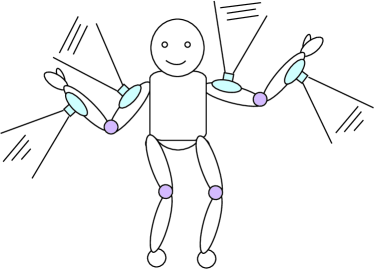
Figure 1: A Robot with Four Cameras Attached on It, Where the Cameras are Articulated.

In hand-eye calibration, it is demonstrated that when a sensor is mounted on a moving robot hand, the relationship between the sensor coordinate system and hand coordinate system can be calculated by the motion information of the hand and the sensor [19, 13, 16]. One example of using kinematic information of the cameras for RMCS is discussed by Caspi and Irani [6], they indicated that if the cameras of a non-overlapping view RMCS are close to each other and share a same projection center, their recorded image sequences can be aligned effectively by the estimated transformations inside each image sequence.

However, in some types of MCS, the relative poses between the cameras are not fixed, hence the calibration methods for the RMCS cannot be used directly. In Figure 1, a novel application of limb pose estimation by attaching cameras on the arms of a robot is shown. On each arm of the robot, two cameras are articulated to each other through the elbow joint of the arm. When the robot moves, the relative pose between the cameras may change, while, the coordinate of the elbow joint relative to each camera attached on the corresponding arm is invariant. In this paper, such a type of MCS is named as Articulated Camera System (ACS). The joint of the elbow is named as the joint in the ACS.

ACSs can be easily found in the real world, such as camera systems attached on human, robots and animals. Before using an ACS, it has to be calibrated. However, there are still some unsolved problems: (i) In an ACS with overlapping view, traditional calibration methods cannot estimate the positions of the joints in the ACS. (ii) In a non-overlapping view ACS, neither the positions of the joints in the ACS nor the relative poses between the cameras in the ACS can be estimated by traditional calibration methods.

These considerations in mind motivate us to develop the technologies in this paper. The rest of this paper are organized as follows: Section II and III analysis the constraints in a moving ACS. The corresponding calibration methods are proposed. Section V and VI evaluate the proposed method by simulation and real experiment. In section VII, a brief conclusion and the future plan are presented.

II Calibration of ACS with Overlapping Views

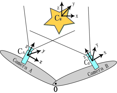
Figure 2: An Articulated Camera System with Overlapping Views

Suppose two rigid objects are articulated at joint O and two cameras (camera A and B) are fixed on the two rigid objects respectively (See Figure 2). Let $C_{A}$ be the coordinate system of camera A, $C_{B}$ the coordinate system of camera B. Suppose there are enough feature correspondences between the cameras so that the pose of $C_{A}$ and $C_{B}$ referring to the same coordinate system $C_{W}$ can be estimated. Therefore, the relative pose between $C_{A}$ and $C_{B}$ is known. We want to find the position of O in the ACS. Let $\mathbf{H}_{AW}$ and $\mathbf{H}_{BW}$ be the Euclidean transformation matrixes describe the $C_{A}$ and $C_{B}$ relative to $C_{W}$, so that for any point $P$:

$$P_{A}=\mathbf{H}_{AW}P_{W}=\left[\begin{array}[]{c c}\mathbf{R}_{AW}&T_{AW}\\ 0&1\end{array}\right]\left[\begin{array}[]{c}\bar{P}_{W}\\ 1\end{array}\right]$$ (1)

$$P_{B}=\mathbf{H}_{BW}P_{W}=\left[\begin{array}[]{c c}\mathbf{R}_{BW}&T_{BW}\\ 0&1\end{array}\right]\left[\begin{array}[]{c}\bar{P}_{W}\\ 1\end{array}\right]$$ (2)

, where $\mathbf{R}$ is the $3\times 3$ rotation matrix, $T$ is a $3\times 1$ vector, $P_{W}$, $P_{A}$ and $P_{B}$ are the homogenous coordinates of the 3-D Point $P$ relative to $C_{W}$, $C_{A}$ and $C_{B}$ respectively, $\bar{P}$ is a $3\times 1$ vector.

According to equations (1) and (2):

$$P_{W}=\mathbf{H}_{AW}^{-1}P_{A}=\mathbf{H}_{BW}^{-1}P_{B}$$ (3)

$$\mathbf{H}_{AW}^{-1}P_{A}-\mathbf{H}_{BW}^{-1}P_{B}=0$$ (4)

$$\left[\begin{array}[]{c c}\mathbf{R}_{AW}^{T}&-\mathbf{R}_{AW}^{T}T_{AW}\\ 0&1\end{array}\right]\left[\begin{array}[]{c}\bar{P}_{A}\\ 1\end{array}\right]-\left[\begin{array}[]{c c}\mathbf{R}_{BW}^{T}&-\mathbf{R}_{BW}^{T}T_{BW}\\ 0&1\end{array}\right]\left[\begin{array}[]{c}\bar{P}_{B}\\ 1\end{array}\right]=0$$ (5)

$$\mathbf{R}_{AW}^{T}\bar{P}_{A}-\mathbf{R}_{BW}^{T}\bar{P}_{B}=\mathbf{R}_{AW}^{T}T_{AW}-\mathbf{R}_{BW}^{T}T_{BW}$$ (6)

, where $\mathbf{R}^{T}$ is the transpose of $\mathbf{R}$. Suppose the ACS performed $n$ transformations. Let $\mathbf{H}_{AW}^{i}$ and $\mathbf{H}_{BW}^{i}$ be the Euclidean transformation matrixes describe the $C_{A}$ and $C_{B}$ relative to $C_{W}$ after the $i$-th transformation of the ACS. According to equation (6):

$$(\mathbf{R}_{AW}^{i})^{T}\bar{P}_{A}-(\mathbf{R}_{BW}^{i})^{T}\bar{P}_{B}=(\mathbf{R}_{AW}^{i})^{T}T_{AW}^{i}-(\mathbf{R}_{BW}^{i})^{T}T_{BW}^{i}$$ (7)

Let $\tilde{O}=\left[\begin{array}[]{cc}\bar{O}_{A}^{T}&\bar{O}_{B}^{T}\end{array}\right]^{T}$, where $\bar{O}_{A}$ and $\bar{O}_{B}$ are the coordinates of the joint O relative to $C_{A}$ and $C_{B}$ respectively. Equation (7) can be rewritten as:

$$\left[\begin{array}[]{cc}(\mathbf{R}_{AW}^{i})^{T}&-(\mathbf{R}_{BW}^{i})^{T}\end{array}\right]\tilde{O}=(\mathbf{R}_{AW}^{i})^{T}T_{AW}^{i}-(\mathbf{R}_{BW}^{i})^{T}T_{BW}^{i}$$ (8)

Since camera A and B are fixed on the articulated rigid objects, $\tilde{O}$ is invariant during the transformation of the ACS. The transformations ($\mathbf{R}_{AW}^{i}$, $\mathbf{R}_{BW}^{i}$, $T_{AW}^{i}$ and $T_{BW}^{i}$ for $i\in[1\dots n]$) of the camera coordinate systems are calculated by the projected image sequences. We propose that $\tilde{O}$ can be estimated by a least squares method, when the ACS has moved to many different positions and captured enough samples of $\mathbf{R}_{AW}^{i}$, $\mathbf{R}_{BW}^{i}$, $T_{AW}^{i}$ and $T_{BW}^{i}$.

The above derivation shows that although the location of the joint $O_{W}^{i}$ in world coordinates is not constant, it equals $(H_{AW}^{i})^{-1}O_{A}$ or $(H_{BW}^{i})^{-1}O_{B}$ because the cameras can not move completely independent as they are connected with a joint. The joint location can be calculated by the 1D subspace intersection of the camera transformation matrices.

III Calibration of Non-Overlapping View ACS

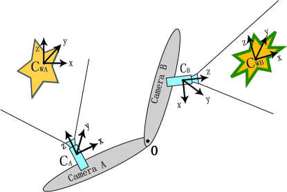
Figure 3: A Non-overlapping View Articulated Camera System

In many situations, there is no overlapping view between the cameras in an ACS. And the lack of common features makes the calibration method proposed in section II become invalid (See Figure 3). Moreover, since the relative pose between the cameras in the ACS cannot be estimated by the overlapping views, the calibration of the relative poses between the non-overlapping view cameras is also required. In this section, a calibration method based on the ego-motion information of the cameras in an ACS is discussed.

III-A Recovering the Position of the Joint Relative to the Cameras in the ACS

Let $C_{A}^{init}$ and $C_{B}^{init}$ be the coordinate systems of camera A and B respectively at the initial state (time $t=0$). Suppose the ACS performs $n$ transformations. Since the coordinate of the joint O relative to camera A is fixed during the transformation of the ACS. At time $t=i$, we have:

$$O_{A}^{i}=\mathbf{H}_{A}^{i}O_{A}=\left[{{\begin{array}[]{cc}\mathbf{R}_{A}^{i}&T_{A}^{i}\\ {0}&{1}\\ \end{array}}}\right]{O}_{A}$$ (9)

, where $\mathbf{H}_{A}^{i}$ is the Euclidean transformation matrix of camera A at time $i$ relative to $C_{A}^{init}$. $\mathbf{R}_{A}^{i}$ and $T_{A}^{i}$ describe the orientation and origin of camera A at time $i$ relative to $C_{A}^{init}$. Also $O_{A}$ is the coordinate of point O at initial state relative to $C_{A}^{init}$, and $O_{A}^{i}$ is the coordinate of point O at time $i$ relative to $C_{A}^{init}$.

If the position of the joint O relative to $C_{A}^{init}$ is fixed during the transformations of the ACS, we have: $O_{A}^{i}=O_{A}$, $\forall i\in[1,\dots,n]$. For $i$-th transformation of the ACS, according to equation (9):

$$O_{A}=\mathbf{H}_{A}^{i}O_{A}=\left[{{\begin{array}[]{cc}\mathbf{R}_{A}^{i}&T_{A}^{i}\\ {0}&{1}\\ \end{array}}}\right]{O}_{A}$$ (10)

$$(\mathbf{R}_{A}^{i}-I)\bar{O}_{A}=-T_{A}^{i}$$ (11)

Let $\mathbf{M}_{A}=[(\mathbf{R}_{A}^{1}-I)^{T},(\mathbf{R}_{A}^{2}-I)^{T},\dots,(\mathbf{\mathbf{R}}_{A}^{n}-I)^{T}]^{T}$, $\tilde{T}_{A}=[(T_{A}^{1})^{T},(T_{A}^{2})^{T},\dots,(T_{A}^{n})^{T}]^{T}$, we have:

$$\mathbf{M}_{A}\bar{O}_{A}=-\tilde{T}_{A}$$ (12)

Since the transformations ($\mathbf{R}_{A}^{i}$ and $T_{A}^{i}$, $\forall i\in[1\dots n]$) of camera A can be calculated by the projected image sequence. We propose $\bar{O}_{A}$ can be estimated by a least squares method. Similarly, $\bar{O}_{B}$ can also be estimated. Therefore, $O_{A}$ and $O_{B}$ are recovered.

III-B The Uniqueness of the Joint Pose Estimation

If the different segments of the articulated camera system (ACS) are connected by 1D rotational joints (connected by point rotational joints) and the ACS can perform general transformations, the solution of the joint pose estimation is unique:

For the joint pose estimation method using special motion (in section III-A). Suppose the solution of the joint pose estimation is not unique, there must exist at least two different 3D points $\bar{O}_{1}$ and $\bar{O}_{2}$ satisfy equation (12). We have: $\mathbf{M}_{A}\bar{O}_{1}=-\tilde{T}_{A}$ and $\mathbf{M}_{A}\bar{O}_{2}=-\tilde{T}_{A}$. Therefore, any point $\bar{P}=s\bar{O}_{1}+(1-s)\bar{O}_{2}$ will also satisfy equation (12), where $s$ is an arbitrary scalar. According to the definition of $\bar{P}$, $\bar{P}$ is the point on the line passing through the points $\bar{O}_{1}$ and $\bar{O}_{2}$. Since $\bar{P}$ satisfy equation (12) represents that the position of the point $P$ relative to the camera in the ACS is invariant during the transformation of the ACS, it means the different segments of ACS are connected by the 2D rotational axis instead of the 1D rotational joints. The position of the points on the 2D rotational axis relative to the camera in the ACS is invariant during the transformation of the ACS. However, it conflicts with the assumption. Similarly, the uniqueness of the joint pose estimation method using overlapping views (in section II) can also be verified.

III-C Recovering the Relative Pose Between the Cameras of the Non-overlapping view ACS

Let $\mathbf{H}_{BA}$ be the Euclidean transformation matrix between $C_{A}^{init}$ and $C_{B}^{init}$, so that for any point $P$:

$${P}_{B}=\mathbf{H}_{BA}P_{A}=\left[{{\begin{array}[]{cc}{\mathbf{R}_{BA}}&T_{BA}\\ {0}&{1}\\ \end{array}}}\right]{P}_{A}=\mathbf{H}_{BA}P_{A}$$ (13)

, where $P_{A}$ and $P_{B}$ are the homogenous coordinate of Point $P$ relative to $C_{A}^{init}$ and $C_{B}^{init}$ respectively.

The relative pose ($\tilde{\mathbf{R}}_{BA}$ and $\tilde{T}_{BA}$) between $C_{A}^{init}$ and $C_{B}^{init}$ is defined as:

$$\tilde{\mathbf{R}}_{BA}={\mathbf{R}}_{BA}^{T}$$ (14)

$$\tilde{T}_{BA}=-{\mathbf{R}}_{BA}^{T}{T}_{BA}$$ (15)

Let $O_{B}^{i}$ be the coordinate of joint O at time $i$ relative to $C_{B}^{init}$. Since the coordinate of the joint O relative to camera B is invariant:

$$O_{B}^{i} = \left[{{\begin{array}[]{cc}{\mathbf{R}_{B}^{i}}&{T_{B}^{i}}\\ {0}&{1}\\ \end{array}}}\right]O_{B}$$ (18)

$$= \left[{{\begin{array}[]{cc}{\mathbf{R}_{B}^{i}}&{T_{B}^{i}}\\ {0}&{1}\\ \end{array}}}\right]\left[{{\begin{array}[]{cc}\mathbf{R}_{BA}&T_{BA}\\ {0}&{1}\\ \end{array}}}\right]O_{A}$$ (23)

$$= \left[{{\begin{array}[]{cc}{\mathbf{R}_{B}^{i}\mathbf{R}_{BA}}&\mathbf{R}_{B}^{i}T_{BA}+T_{B}^{i}\\ {0}&{1}\\ \end{array}}}\right]O_{A}$$ (26)

According to equations (9) and (13):

$$O_{B}^{i} = \mathbf{H}_{BA}O_{A}^{i}$$ (31)

$$= \left[\begin{array}[]{cc}\mathbf{R}_{BA}&T_{BA}\\ {0}&{1}\\ \end{array}\right]\left[\begin{array}[]{cc}\mathbf{R}_{A}^{i}&T_{A}^{i}\\ {0}&{1}\\ \end{array}\right]O_{A}$$

$$= \left[{{\begin{array}[]{cc}\mathbf{R}_{BA}{\mathbf{R}}_{A}^{i}&{\mathbf{R}_{BA}T_{A}^{i}+{T_{BA}}}\\ {0}&{1}\\ \end{array}}}\right]{O}_{A}$$ (34)

According to equations (18) and (31):

$$\left[{{\begin{array}[]{cc}{\mathbf{R}_{B}^{i}\mathbf{R}_{BA}}&{\mathbf{R}_{B}^{i}T_{BA}+T_{B}^{i}}\\ {0}&{1}\\ \end{array}}}\right]\left[{{\begin{array}[]{c}\bar{O}_{A}\\ {1}\\ \end{array}}}\right]=\left[{{\begin{array}[]{cc}{\mathbf{R}_{BA}\mathbf{R}_{A}^{i}}&\mathbf{\mathbf{R}}_{BA}T_{A}^{i}+{T_{BA}}\\ {0}&{1}\\ \end{array}}}\right]\left[{{\begin{array}[]{c}\bar{O}_{A}\\ {1}\\ \end{array}}}\right]$$ (35)

$$\left[{{\begin{array}[]{cc}{\mathbf{R}_{B}^{i}\mathbf{R}_{BA}\bar{O}_{A}+\mathbf{R}_{B}^{i}T_{BA}+T_{B}^{i}}\\ {1}\\ \end{array}}}\right]=\left[{{\begin{array}[]{cc}{\mathbf{R}_{BA}\mathbf{R}_{A}^{i}\bar{O}_{A}+\mathbf{R}_{BA}T_{A}^{i}+T_{BA}}\\ {1}\\ \end{array}}}\right]$$ (36)

$$\mathbf{R}_{B}^{i}\mathbf{R}_{BA}\bar{O}_{A}+\mathbf{R}_{B}^{i}T_{BA}-\mathbf{R}_{BA}\mathbf{R}_{A}^{i}\bar{O}_{A}-\mathbf{R}_{BA}T_{A}^{i}+T_{B}^{i}-T_{BA}=0$$ (37)

Since $\bar{O}_{A}$ can be estimated by the method discussed in section III-C, the $\mathbf{R}_{BA}$ and $T_{BA}$ can be estimated by a least square method, when the ACS perform enough general motions.

In our simulation and real experiment, the estimated $R_{BA}$ is refined by a method discussed in [20]. Then the roll, pitch and yaw corresponding to the $R_{BA}$ are estimated according to the definition of the rotation matrix [11]. Let $R_{BA}=M(r,p,y)$, where $r$ $p$ and $y$ are the corresponding roll, pitch and yaw of $\mathbf{R}_{BA}$, $M$ is a function from roll, pitch and yaw to the corresponding rotation matrix. Then, the $r$, $p$, $y$, $T_{BA}$ and $\bar{O}_{A}$ are optimized by minimizing the nonlinear error function:

$$E(r,p,y,T_{BA},O_{A})=\sum_{i=1}^{n}(\mathbf{R}_{B}^{i}M(r,p,y)\bar{O}_{A}+\mathbf{R}_{B}^{i}T_{BA}$$

$$-M(r,p,y)\mathbf{R}_{A}^{i}\bar{O}_{A}-M(r,p,y)T_{A}^{i}+T_{B}^{i}-T_{BA})$$ (38)

using a Levenberg-Marquardt method. Finally, the $R_{BA}$ is recovered from the optimized $r$, $p$ and $y$. The relative pose between the $C_{A}^{init}$ and $C_{B}^{init}$ is calculated by equations (14) and (15).

IV Dealing With Unknown Scale Factors

The non-overlapping view ACS calibration method discussed above depends on the ego-motion information of the cameras in the ACS. However, if the model of the scene is unknown, the estimated ego-translations of the cameras may be scaled by different unknown scale factors. These unknown scale factors must be considered in the extrinsic calibration process.

IV-A Model Analysis

Let $T_{A}$ and $T_{B}$ be the true ego-translation of camera A and B in the world coordinate system, $\hat{T}_{A}$ and $\hat{T}_{B}$ be the estimated ego-translations of camera A and B found by an SFM method, $\mu_{A}$ and $\mu_{B}$ be the corresponding unknown scale factors. So that:

$$\hat{T}_{A}=\mu_{A}T_{A}$$ (39)

$$\hat{T}_{B}=\mu_{B}T_{B}$$ (40)

Let $\hat{\bar{O}}_{A}$ be the pose of the joint relative to $C_{A}$ calculated with the estimated motion. Equation (11) can be rewritten as:

$$(\mathbf{R}_{A}^{i}-I)\hat{\bar{O}}_{A}=-\hat{T}_{A}^{i}=-\mu_{A}T_{A}^{i}$$ (41)

$$(\mathbf{R}_{A}^{i}-I)\frac{\hat{\bar{O}}_{A}}{\mu_{A}}=-T_{A}^{i}$$ (42)

Compare equation (42) with equation (11), we have:

$$\hat{\bar{O}}_{A}=\mu_{A}\bar{O}_{A}$$ (43)

Let $\hat{\mathbf{R}}_{BA}$ and $\hat{T}_{BA}$ be the extrinsic parameters calculated using the estimated motions and joint pose. Equation (37) can be rewritten as:

$$\mathbf{R}_{B}^{i}\hat{\mathbf{R}}_{BA}\hat{\bar{O}}_{A}+\mathbf{R}_{B}^{i}\hat{T}_{BA}-\hat{\mathbf{R}}_{BA}\mathbf{R}_{A}^{i}\hat{\bar{O}}_{A}-\hat{\mathbf{R}}_{BA}\hat{T}_{A}^{i}+\hat{T}_{B}^{i}-\hat{T}_{BA}=0$$ (44)

According to equation (39), (40), (43) and (44):

$$\mathbf{R}_{B}^{i}\hat{\mathbf{R}}_{BA}\mu_{A}\bar{O}_{A}+\mathbf{R}_{B}^{i}\hat{T}_{BA}-\hat{\mathbf{R}}_{BA}\mathbf{R}_{A}^{i}\mu_{A}\bar{O}_{A}-\hat{\mathbf{R}}_{BA}\mu_{A}{T}_{A}^{i}+\mu_{B}{T}_{B}^{i}-\hat{T}_{BA}=0$$ (45)

$$\mathbf{R}_{B}^{i}\frac{\mu_{A}}{\mu_{B}}\hat{\mathbf{R}}_{BA}\bar{O}_{A}+\mathbf{R}_{B}^{i}\frac{1}{\mu_{B}}\hat{T}_{BA}-\frac{\mu_{A}}{\mu_{B}}\hat{\mathbf{R}}_{BA}\mathbf{R}_{A}^{i}\bar{O}_{A}-\frac{\mu_{A}}{\mu_{B}}\hat{\mathbf{R}}_{BA}{T}_{A}^{i}+{T}_{B}^{i}-\frac{1}{\mu_{B}}\hat{T}_{BA}=0$$ (46)

Let:

$$\frac{\mu_{A}}{\mu_{B}}\hat{\mathbf{R}}_{BA}=\mathbf{\breve{R}}_{BA}$$ (47)

$$\frac{1}{\mu_{B}}\hat{T}_{BA}=\breve{T}_{BA}$$ (48)

Equation (46) can be rewritten as:

$$\mathbf{R}_{B}^{i}\breve{\mathbf{R}}_{BA}\bar{O}_{A}+\mathbf{R}_{B}^{i}\breve{T}_{BA}-\breve{\mathbf{R}}_{BA}\mathbf{R}_{A}^{i}\bar{O}_{A}-\breve{\mathbf{R}}_{BA}{T}_{A}^{i}+{T}_{B}^{i}-\breve{T}_{BA}=0$$ (49)

Since the equations (49) and (37) are exactly the same, we have:

$$\mathbf{R}_{BA}=\breve{\mathbf{R}}_{BA}$$ (50)

$$T_{BA}=\breve{T}_{BA}$$ (51)

Therefore:

$$\hat{\mathbf{R}}_{BA}=\frac{\mu_{B}}{\mu_{A}}\mathbf{\breve{R}}_{BA}=\phi_{BA}\mathbf{R}_{BA}$$ (52)

$$\hat{T}_{BA}={\mu_{B}}\breve{T}_{BA}={\mu_{B}}T_{BA}$$ (53)

Where $\phi_{BA}=\frac{\mu_{B}}{\mu_{A}}$. Equations (52) and (53) show that the estimated rotation matrix $\hat{\mathbf{R}}_{BA}$ will be scaled by the relative scale factor (the ratio of the scale factors of the cameras) and the estimated relative translation will be scaled by the same scale factor of camera $B$. In the next section, we will discuss the estimation of the relative scale factor.

IV-B Rotation Matrix and Relative Scale Factor Estimation

Let $\mathbf{R}^{\prime}=\phi\mathbf{R}+N$, where $\mathbf{R}$ is a $3\times 3$ rotation matrix and $\mathbf{R}^{T}\mathbf{R}=I$, $\phi$ is an unknown scale factor, $N$ is a $3\times 3$ unknown noise matrix. We want to recover $\mathbf{R}$ and $\phi$ from $\mathbf{R}^{\prime}$. According to the definition, we have:

$$\mathbf{R}^{\prime}=\phi\mathbf{R}+N=\phi(\mathbf{R}+\frac{N}{\phi})=\phi M$$ (54)

Where $M=\mathbf{R}+\frac{N}{\phi}$.

Let the singular value decomposition of $M$ be $UDV^{T}$, where $D=diag(\sigma_{1},\sigma_{2},\sigma_{3})$. As illustrated in appendix C of [20], $r$ can be approximated by:

$$\mathbf{R}=UV^{T}$$ (55)

Now, let the singular value decomposition of $r^{\prime}$ be $\tilde{U}\tilde{D}\tilde{V}^{T}$, since $\mathbf{R}^{\prime}=\phi M$, we have:

$$\tilde{U}=U$$ (56)

$$\tilde{V}=V$$ (57)

$$\tilde{D}=\phi D$$ (58)

Combine equations (55), (56) and (57), the rotation matrix $r$ can be recovered by:

$$\mathbf{R}=\tilde{U}\tilde{V}^{T}$$ (59)

When noise $N$ is not significant, $D\approx I_{3\times 3}$, the scale factor $\phi$ can be estimated by the following approximation:

$$trace(\tilde{D})=trace(\phi D)\approx trace(\phi I_{3\times 3})\approx 3\phi$$ (60)

$$\phi\approx\frac{1}{3}trace(\tilde{D})$$ (61)

In short, if we have enough samples of $\mathbf{R}_{A}^{i}$, $\hat{T}_{A}^{i}$, $\mathbf{R}_{B}^{i}$ and $\hat{T}_{B}^{i}$ we can find $\hat{O}_{A}$, $\hat{\mathbf{R}}_{BA}$ and $\hat{T}_{BA}$(see section IV-A). Then using the above formulas, in particular, equation (59) and (61), we can also find the real rotation ($\mathbf{R}_{BA}$) and the relative scale factor $\phi_{BA}$.

Let $\mathbf{R}_{BA}=M(r,p,y)$, where $r$, $p$ and $y$ are the corresponding roll, pitch and yaw of $\mathbf{R}_{BA}$, $M$ is a function from roll, pitch and yaw to the corresponding rotation matrix. In our simulation and real experiment, the estimated $r$, $p$, $y$, $\hat{T}_{BA}$ and $\phi_{BA}$ can be optimized by minimizing the nonlinear error function:

$$E(r,p,y,T_{BA},Q_{A})=\sum_{i=1}^{n}(\phi_{BA}R_{B}^{i}M(r,p,y)\hat{\bar{O}}_{A}+R_{B}^{i}\hat{T}_{BA}-\phi_{BA}M(r,p,y)R_{A}^{i}\hat{\bar{O}}_{A}-\phi_{BA}M(r,p,y)T_{A}^{i}+\hat{T}_{B}^{i}-\hat{T}_{BA})$$ (62)

using a Levenberg-Marquardt method. If the pose of the joint is calibrated with known scale factor ($O_{A}$ is known), the scale factor $\mu_{A}$ can be estimated by equation (43). The scale factor $\mu_{B}$ can be calculated by $\frac{\mu_{A}}{\phi_{BA}}$. Finally, the $\mathbf{R}_{BA}$ is recovered from the optimized $r$, $p$ and $y$. The relative pose between the $C_{A}^{init}$ and $C_{B}^{init}$ is calculated by equations (14) and (15). Therefore, a non-overlapping view ACS can also be calibrated using scaled motion information from each camera in it.

V Simulation

In this section, the proposed calibration methods are evaluated with synthetic transformation data.

V-A Performance w.r.t. Noise in Transformation Data

Setup and Notations: In each test, one ACS with 2 cameras and 1 joint is generated randomly. In which, $1\leq|O_{A}|\leq 2$ meters, $1\leq|O_{B}|\leq 2$ meters. The generated ACS performs $30$ random transformations.

Performance of the Calibration Method for ACS with Overlapping Views: In the first simulation, the proposed algorithm is tested 100 times. Zero mean Gaussian noise is added to the transformation data of the cameras. The configuration, input and output of our simulation system are list as Table I. Since we assume there are overlapping views between the two cameras, the relative pose between them can be estimated by many existing methods as discussed in section I. Only the performance of joint pose estimation is evaluated in our simulation. The error of joint estimation are computed by:

$$Err=\frac{|\bar{O}_{A}-\hat{\bar{O}}_{A}|}{2|\bar{O}_{A}|}+\frac{|\bar{O}_{B}-\hat{\bar{O}}_{B}|}{2|\bar{O}_{B}|}$$ (63)

, where $\bar{O}_{A}$ is the ground truth, $\hat{\bar{O}}_{A}$ is the estimated position of joint O relative to camera A. Similarly, $\bar{O}_{B}$ is the ground truth, $\hat{\bar{O}}_{B}$ is the estimated position of joint O relative to camera B. The corresponding results are shown in Figure 4.

TABLE I: Configuration, Input and Output

Configuration
No. of Cameras in the ACS	2
No. of Joints in the ACS	1
Random transformations per test (n)	30
Number of tests	100
Input ($i=1\dots n$)
Rotations of cameras ($\mathbf{R}_{AW}^{i}$, $\mathbf{R}_{BW}^{i}$)	$2\times 30\times 100$
Translations of cameras ($T_{AW}^{i}$, $T_{BW}^{i}$)	$2\times 30\times 100$
Zero Mean Gaussian noise:
$0\leq\sigma_{rot}\leq 2.4^{\circ}$ and $0\leq\sigma_{trans}\leq 0.1meters$
Output
Mean error of joint pose estimation (see equation (63))
STD error of joint pose estimation (see equation (63))

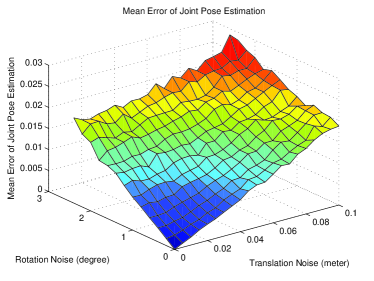
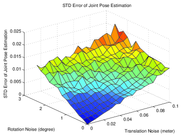
(a)	(b)

Figure 4: Mean and STD Error of Joint Pose ($O_{A}$) Estimation. (a) Mean Error of Joint Pose Estimation; (b) STD Error of Joint Pose.

Performance of the Calibration Method for Non-Overlapping Views ACS: In the second simulation, firstly, the pose of the joint is fixed relative to $C_{A}^{init}$ during the transformations of the ACS. The pose of the joint relative to the camera A ($O_{A}$) is calibrated by the transformations of camera A. Similarly, $O_{B}$ is calibrated. Then, the ACS performs several general transformations (the joint is not needed to be fixed relative to $C_{A}^{init}$), the relative pose between the cameras are calibrated using the estimated joint pose and the transformations of the cameras. The configuration, input and output of the simulation system are listed as Table II. The error of joint pose, relative rotation, relative translation estimation are calculated by equation (63), (64) and (65) respectively.

Figure 5 shows the results of joint pose estimation. Compare with the calibration method using the overlapping views, the calibration method using special motions is more accurate. The mean and STD error of the relative rotation and translation estimation are presented in Figure 6 and 7. The proposed algorithms are shown to be stable, when the zero mean Gaussian noise from $0^{\circ}$ to $2.4^{\circ}$ is added to the roll, pitch and yaw of the rotation data, and the zero mean Gaussian noise from $0$ to $0.1$ meters is added to the translation data.

$$Err^{rot}=\sqrt{|roll-\widehat{roll}|^{2}+|pitch-\widehat{pitch}|^{2}+|yaw-\widehat{yaw}|^{2}}$$ (64)

$$Err^{trans}=\frac{|T_{AB}-\hat{T}_{AB}|}{|T_{AB}|}$$ (65)

TABLE II: Configuration, Input and Output

Configuration
No. of Cameras in the ACS	2
No. of Joints in the ACS	1
Random transformations per test (n)	30
Number of tests	100
Input ($i=1\dots n$)
Transformations with fixed joint pose:
Rotations of cameras ($\mathbf{R}_{A}^{i}$, $\mathbf{R}_{B}^{i}$)	$2\times 30\times 100$
Translations of cameras ($T_{A}^{i}$, $T_{B}^{i}$)	$2\times 30\times 100$
General transformations:
Rotations of cameras ($\mathbf{R}_{A}^{i}$, $\mathbf{R}_{B}^{i}$)	$2\times 30\times 100$
Translations of cameras ($T_{A}^{i}$, $T_{B}^{i}$)	$2\times 30\times 100$
Zero Mean Gaussian noise:
$0\leq\sigma_{rot}\leq 2.4^{\circ}$ and $0\leq\sigma_{trans}\leq 0.1meters$
Output
Mean error of joint pose estimation (see equation (63))
STD error of joint pose estimation (see equation (63))
Mean error of relative translation estimation (see equation (65))
STD error of relative translation estimation (see equation (65))
Mean error of relative rotation estimation (see equation (64))
STD error of relative rotation estimation (see equation (64))

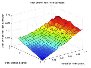
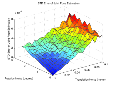
(a)	(b)

Figure 5: Mean and STD Error of Joint Pose ($\hat{O}_{A}$) Estimation. (a) Mean Error of Joint Pose Estimation; (b) STD Error of Joint Pose Estimation.

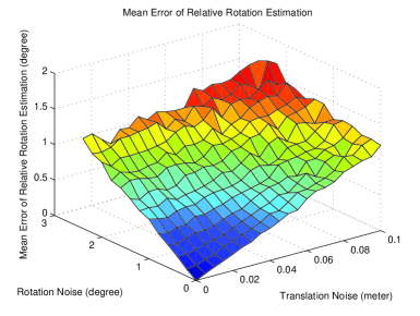
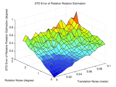
(a)	(b)

Figure 6: Mean and STD Error of Relative Rotation ($R_{BA}$) Estimation. (a) Mean Error of Relative Rotation Estimation; (b) STD Error of Relative Rotation Estimation.

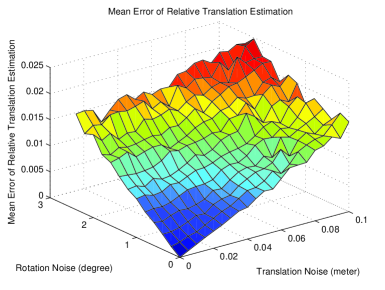
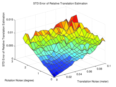
(a)	(b)

Figure 7: Mean and STD Error of Relative Translation ($\hat{T}_{BA}$) Estimation. (a) Mean Error of Relative Translation Estimation; (b) STD Error of Relative Translation Estimation.

Performance of the Calibration Method for Non-Overlapping Views ACS with Unknown Scale Factors: The scale factors of the two cameras in each test are assumed to be uniform distributed in the range $[0.5,5]$. Therefore, the relative scale factor between the two cameras satisfies the uniform distribution in the range of $[0.1,10]$. The joint pose of the ACS is generate randomly and estimated by the method described in section III-A. Other configurations are the same as the second simulation. The $\hat{O}_{A}$, $R_{BA}$, $\hat{T}_{BA}$ and $\phi_{BA}$ are estimated and optimized as discussed in section IV. The error of joint pose, relative rotation, relative translation estimation are calculated by equation (63), (64) and (65) respectively. The error of relative scale factor estimation is evaluated by $\varepsilon_{\phi}=\frac{|\phi-\hat{\phi|}}{|\phi|}$. Where $\hat{\phi}$ is the estimated relative scale factor, and $\phi$ is the ground truth.

Figure 9 and 10 show the results of the relative pose estimation. Compared to figure 6 and 7 the accuracies are similar.

Figure 11 shows the performance of the relative scale factor estimation. The accuracy of the relative scale factor estimation $[(1-\varepsilon_{\phi})\times 100\%]$ is no less than $98.5\%$, when the standard derivation of the noise in ego-rotation is less than $3^{\circ}$ and the standard derivation of the noise in ego-translation is less than $0.1$ meters.

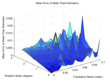
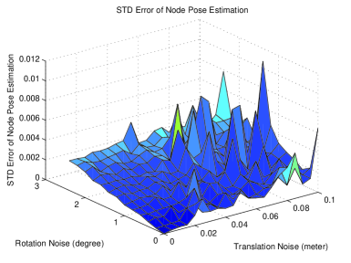
(a)	(b)

Figure 8: Mean and STD Error of Joint Pose with Unknown Scale Factor ($\hat{O}_{A}$). (a) Mean Error of Joint Pose; (b) STD Error of Joint Pose.

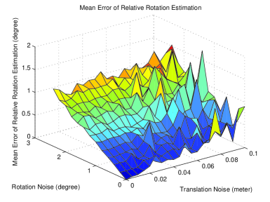
(a)	(b)

Figure 9: Mean and STD Error of Relative Rotation with Unknown Scale Factor $(R_{BA})$. (a) Mean Error of Relative Rotation; (b) STD Error of Relative Rotation.

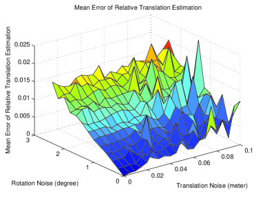
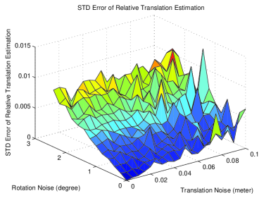
(a)	(b)

Figure 10: Mean and STD Error of Relative Translation with Unknown Scale Factor ($\hat{T}_{BA}$). (a) Mean Error of Relative Translation; (b) STD Error of Relative Translation.

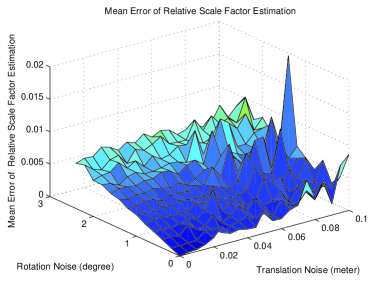
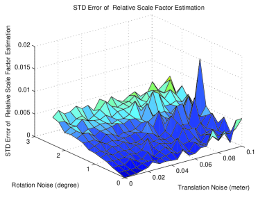
(a)	(b)

Figure 11: Mean and STD Error of Relative Scale Factor with Unknown Scale Factor ($\phi_{BA}$). (a) Mean Error of Relative Scale Factor; (b) STD Error of Relative Scale Factor.

VI Real Experiment

In the real experiments, an ACS with two cameras (Cannon PowerShot G9) is set up as Figure 13 (a). The intrinsic parameters of each camera in the ACS are calibrated by Bouguet’s implementation (“Camera Calibration Toolbox for Matlab”) of [21]. Since the Bouguet’s Toolbox can also estimate the pose information of the camera, the transformations of each camera are calculated using the same image sequence for the intrinsic calibration simultaneously. No additional images nor manual input is required in the real experiments.

VI-A Calibration of the Pose of the Joint in Each Camera

By Overlapping Views (Algorithm I): In the first real experiment, the two cameras in the ACS observe the same checker plane and record images simultaneously. The two cameras are free to move during the transformation of the ACS. Two image sequences ($Q_{1}$ and $Q_{2}$) are recorded, each sequence consists of $15$ images of size $1600\times 1200$ pixels. The estimated joint pose are list in Table III as algorithm I.

By Fixed-Joint Motions (Algorithm II): In the second real experiment, the joint of the ACS is fixed relative to the world coordinate system during the transformation of the ACS. The two cameras do not need to view the same checker plane. And each camera records the image sequence independently. Two image sequences ($Q_{3}$ and $Q_{4}$) are recorded, each sequence consists of $12$ images of size $1600\times 1200$ pixels. The camera pose of the first image is selected as the initial pose to generate the transformation sequence of each camera. The estimated joint pose are list in Table III as algorithm II. The poses of the joint relative to the two cameras in the ACS are also estimated manually for comparison purpose. Since the camera pose of any image in each image sequence can be chosen as the initial camera pose (see section III-A), the proposed algorithm is also tested by choosing different images as the reference. The mean and standard derivation of the corresponding calibration results are presented in Table IV.

TABLE III: Results Of Joint Pose Calibration

I: the algorithm using overlapping views. (see section VI-A) II: the algorithm using fixed-joint motions. (see section VI-A) M: manual measurement(ground truth). $O_{A}$ is the coordinate of the joint relative to camera A, the same applies to $O_{B}$.

Algorithm		Joint Pose (mm)
		X	Y	Z
I	${O}_{A}$	300.28	50.07	-33.47
	${O}_{B}$	-273.70	53.81	-30.15
II	${O}_{A}$	304.55	47.64	-37.66
	${O}_{B}$	-265	54.41	-35.48
M	${O}_{A}$	300 $\pm$ 10	50$\pm$ 10	-40$\pm$ 10
	${O}_{B}$	-270$\pm$ 10	50$\pm$ 10	-30$\pm$ 10

TABLE IV: Mean and STD of the Joint Pose Calibration Algorithm II Using Different Reference Images

$O_{A}$ is the coordinate of the joint relative to camera A, the same applies to $O_{B}$.
Algorithm Joint Pose (mm) II X Y Z Mean ${O}_{A}$ 305.44 47.19 -39.2 ${O}_{B}$ -262.97 56.21 -39.20 STD ${O}_{A}$ 1.89 1.16 3.02 ${O}_{B}$ 3.3 2.67 2.58

VI-B Calibration of Relative Pose Between the Cameras in the Non-Overlapping View ACS (Algorithm III)

In the third real experiment, firstly, we use the non-overlapping view ACS calibration method to process the image sequences $Q_{1}$ and $Q_{2}$. The joint pose (${\bar{O}}_{A}$) estimated by algorithm II is used as the input for the relative pose calibration. Since there are overlapping views between $Q_{1}$ and $Q_{2}$, we also calibrate the relative pose between the two cameras by the feature correspondences for comparison. The calibration result are listed in Table V. After the joint pose relative to each camera in the ACS and relative pose between the cameras in the ACS are calibrated, the trajectory of the ACS is recovered (see Figure 12).

TABLE V: Result of Relative Pose Calibration

III: our method. (see section VI-B) F: using feature correspondences.
Algorithm Relative Rotation (Degree) Roll Pitch Yaw III 17.7158 -11.3660 -80.1913 F 17.5459 -10.6024 -78.9854 Algorithm Relative Translation (mm) $T_{x}$ $T_{y}$ $T_{z}$ III 295.4183 -232.4576 34.5004 F 294.0235 -229.8369 28.9739

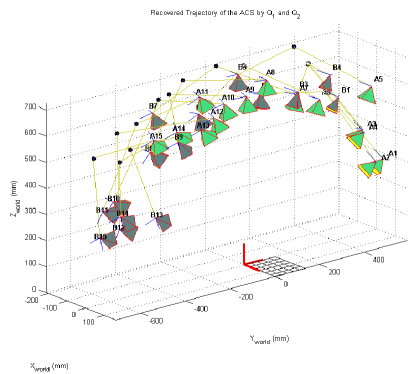
Figure 12: The Trajectory of the ACS Recovered from $Q_{1}$ and $Q_{2}$

The proposed calibration method is also tested by non-overlapping view image sequences. Figure 13 (b), (c), (d) shows the configuration of the non-overlapping view ACS calibration system in the real experiment. Two image sequences ($Q_{5}$ and $Q_{6}$) are recorded, each sequence consists of $17$ images of size $1600\times 1200$ pixels. There is no overlapping view between $Q_{5}$ and $Q_{6}$. Figure 14 shows some samples of the recorded images. We also manually measured the relative pose between the two cameras for comparison. Since no feature correspondence can be used, we only get a rough estimation by a ruler. The calibration results are shown in Table VI. After the relative pose between the cameras at the initial state is estimated, the trajectory of the non-overlapping view ACS is recovered (see Figure 15).

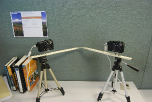
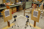
(a)	(b)
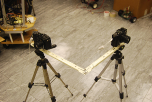
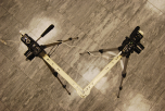
(c)	(d)

Figure 13: The ACS with Two Cannon PowerShot G9 Used in the Real Experiment. (a) The ACS Used in the Real Experiment. (b) The ACS and two Checker Planes. (c) In the Front of the ACS. (d) On the Top of the ACS.

Img1	Img6	Img12	Img17

(a) Images Recorded by Camera A
Img₁ Img₆ Img₁₂ Img₁₇
(b) Images Recorded by Camera B

Figure 14: Images Recorded by the ACS

TABLE VI: Result of Relative Pose Calibration Using Non-Overlapping View Image Sequences

III: our method. (see section VI-B) M: manual measurement
 
  Algorithm Relative Rotation (Degree) Roll Pitch Yaw III 1.3182 88.4530 0.7315 M 0 $\pm$ 5 90 $\pm$ 5 0 $\pm$ 5 Algorithm Relative Translation (mm) $T_{x}$ $T_{y}$ $T_{z}$ III 291.3321 -17.2837 -292.1382 M 290$\pm$20 0 $\pm$ 20 280 $\pm$20

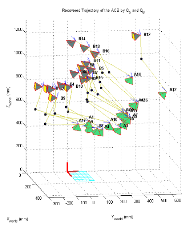
Figure 15: The Trajectory of the ACS Recovered from $Q_{5}$ and $Q_{6}$

VI-C Calibration of Relative Pose Between the Cameras in the Non-Overlapping View ACS with Unknown Scale Factors (Algorithm IV)

The scale factor estimation algorithm is evaluated in the fourth real experiment. The estimated translations from $Q_{1}$ and $Q_{2}$ are multiplied by $0.8$ and $3.2$ respectively. In this case, if no noise exists, the estimated relative scale factor ($\phi_{BA}$) should be $4$. The estimated relative scale factor ($\hat{\phi}_{BA}$) in our experiment was $3.8919$. Table VII lists the corresponding results, in which the estimated relative translations are divided by $3.2$, so that they can be easily compared with the estimated relative translations in Table V. The experiment showed that our algorithms can estimate the relative scale factor and find the extrinsic parameters correctly. In order to test the stability of the scale factor estimation algorithm, the estimated translations from $Q_{5}$ and $Q_{6}$ are multiplied by $0.8$ and $3.2$ respectively. $100$ tests are performed. In each test, $22$ images are randomly selected as section VI-B. The Mean and STD of the calibration results is listed in Table VIII. The results are good.

TABLE VII: Result of Relative Pose Calibration with Unknown Scale Factors (0.8 in $Q_{1}$ and 3.2 in $Q_{2}$ )

IV: our scale factor estimation method. (see section VI-C) F: using feature correspondences.

Algorithm	Relative Rotation (Degree)
	Roll	Pitch	Yaw
IV	17.4883	-10.5185	-79.2551
F	17.5459	-10.6024	-78.9854
Algorithm	Relative Translation (mm)
	$T_{x}$	$T_{y}$	$T_{z}$
IV	295.9218	-220.6804	11.5566
F	294.0235	-229.8369	28.9739

TABLE VIII: Mean and STD of the Relative Pose Calibration Using Non-Overlapping View Image Sequences with Unknown Scale Factors. ($Q_{5}$ and $Q_{6}$) (see section VI-C)

Algorithm	Relative Rotation (Degree)
IV	Roll	Pitch	Yaw
Mean	-4.4275	38.9820	-14.3572
STD	0.4304	0.2639	0.5774
Algorithm	Relative Translation (mm)
IV	$T_{x}$	$T_{y}$	$T_{z}$
Mean	489.2497	-56.0786	-165.7425
STD	6.2496	3.1070	3.7616
Algorithm	Relative Scale Factor
IV	$\phi_{BA}$
Mean	3.9531
STD	0.0159

VII Conclusion

In this paper, an ACS calibration method is developed. Both the simulation and real experiment show that the pose of the joint in an ACS can be estimated robustly. When there is no overlapping view between the cameras in an ACS, the joint pose and the relative pose between the cameras can also be calculated. The trajectory of an ACS can be recovered after the ACS is calibrated. The proposed calibration method requires only the image sequences recorded by the cameras in the ACS. A scale factor estimation algorithm is proposed to deal with unknown scale factors in the estimated translation information of the cameras in an ACS. In the real experiment, the intrinsic and extrinsic parameters of the ACS are calibrated using the same image sequences simultaneously.

Since we still cannot find any former study of the ACS calibration in the literature. We apologize for having no comparison with former ACS calibration method.

Our future plan may focus on using an ACS attached on different parts of human body to track the motion of the human. We foresee that if calibration of articulated cameras become a simple routine, researchers will find many novel and interesting applications for such a camera system.

References

- [1] M. Antone and S. Teller. Scalable extrinsic calibration of omni-directional image networks. International Journal of Computer Vision, 49(2):143–174, 2002.
- [2] P. Baker and Y. Aloimonos. Complete calibration of a multi-camera network. Proc. IEEE Workshop on Omnidirectional Vision, 12:134–141, 2000.
- [3] P. Baker, A. Ogale, and C. Fermuller. The Argus eye: a new imaging system designed to facilitate robotic tasks of motion. Robotics & Automation Magazine, IEEE, 11(4):31–38, 2004.
- [4] P. T. Baker and Y. Aloimonos. Calibration of a multicamera network. Conference on Computer Vision and Pattern Recognition Workshop, 07:72, 2003.
- [5] B. Caprile and V. Torre. Using vanishing points for camera calibration. International Journal of Computer Vision, 4(2):127–139, 1990.
- [6] Y. Caspi and M. Irani. Aligning Non-Overlapping Sequences. International Journal of Computer Vision, 48(1):39–51, 2002.
- [7] S. Dockstader and A. Tekalp. Multiple camera tracking of interacting and occluded human motion. Proceedings of the IEEE, 89(10):1441–1455, 2001.
- [8] F. Dornaika. Self-calibration of a stereo rig using monocular epipolar geometries. Pattern Recognition, 40(10):2716–2729, 2007.
- [9] Y. Furukawa and J. Ponce. Accurate camera calibration from multi-view stereo and bundle adjustment. International Journal of Computer Vision, 84(3):257–268, 2009.
- [10] R. R. Garcia and A. Zakhor. Geometric calibration for a multi-camera-projector system. In WACV, pages 467–474, 2013.
- [11] R. I. Hartley and A. Zisserman. Multiple view geometry in computer vision. Cambridge University Press, ISBN: 0521540518, second edition, 2004.
- [12] J. Heikkila and O. Silven. A four-step camera calibration procedure with implicit imagecorrection. Computer Vision and Pattern Recognition, 1997. Proceedings., 1997 IEEE Computer Society Conference on, pages 1106–1112, 1997.
- [13] R. Horaud and F. Dornaika. Hand-eye calibration. International Journal of Robotics Research, 14(3):195–210, 1995.
- [14] M. Kaess and F. Dellaert. Visual SLAM with a Multi-Camera Rig. Technical report, Georgia Institute of Technology, 2006.
- [15] H. G. Maas. Image sequence based automatic multi-camera system calibration techniques. In International Archives of Photogrammetry and Remote Sensing, 32(B5):763–768, 1998.
- [16] A. Malti. Hand-eye calibration with epipolar constraints: Application to endoscopy. Robotics and Autonomous Systems, 2012.
- [17] E. Morais, A. Ferreira, S. A. Cunha, R. M. Barros, A. Rocha, and S. Goldenstein. A multiple camera methodology for automatic localization and tracking of futsal players. Pattern Recognition Letters, 2013.
- [18] S. Shah and J. Aggarwal. Intrinsic parameter calibration procedure for a (high-distortion) fish-eye lens camera with distortion model and accuracy estimation*. Pattern Recognition, 29(11):1775–1788, 1996.
- [19] R. Tsai and R. Lenz. A new technique for fully autonomous and efficient 3D roboticshand/eye calibration. Robotics and Automation, IEEE Transactions on, 5(3):345–358, 1989.
- [20] Z. Zhang. A flexible new technique for camera calibration. Technical report, Technical Report MSR-TR-98-71, Microsoft Research, 1998.
- [21] Z. Zhang. A flexible new technique for camera calibration. IEEE Transactions on Pattern Analysis and Machine Intelligence, 22(11):1330–1334, 2000.