Insights into the Phase Diagram of Bismuth Ferrite from Quasi-Harmonic Free Energy Calculations

Abstract

We have used first-principles methods to investigate the phase diagram of multiferroic bismuth ferrite (BiFeO₃ or BFO), revealing the energetic and vibrational features that control the occurrence of various relevant structures. More precisely, we have studied the relative stability of four low-energy BFO polymorphs by computing their free energies within the quasi-harmonic approximation, introducing a practical scheme that allows us to account for the main effects of spin disorder. As expected, we find that the ferroelectric ground state of the material (with $R3c$ space group) transforms into an orthorhombic paraelectric phase ($Pnma$) upon heating. We show that this transition is not significantly affected by magnetic disorder, and that the occurrence of the $Pnma$ structure relies on its being vibrationally (although not elastically) softer than the $R3c$ phase. We also investigate a representative member of the family of nano-twinned polymorphs recently predicted for BFO [Prosandeev et al., Adv. Funct. Mater. 23, 234 (2013)] and discuss their possible stabilization at the boundaries separating the $R3c$ and $Pnma$ regions in the corresponding pressure-temperature phase diagram. Finally, we elucidate the intriguing case of the so-called super-tetragonal phases of BFO: Our results explain why such structures have never been observed in the bulk material, despite their being stable polymorphs of very low energy. Quantitative comparison with experiment is provided whenever possible, and the relative importance of various physical effects (zero-point motion, spin fluctuations, thermal expansion) and technical features (employed exchange-correlation energy density functional) is discussed. Our work attests the validity and usefulness of the quasi-harmonic scheme to investigate the phase diagram of this complex oxide, and prospective applications are discussed.

I Introduction

Magnetoelectric multiferroics, a class of materials in which ferroelectric and (anti-)ferromagnetic orders coexist, are generating a flurry of interest because of their fundamental complexity and potential for applications in electronics and data-storage devices, among others. In particular, the magnetoelectric coupling between their magnetic and electric degrees of freedom opens the possibility for the control of the magnetization via the application of a bias voltage in advanced spintronic devices.fiebig05 ; fiebig06 ; ramesh07 ; eerenstein06 ; balke12 ; rovillain10 ; gajek07

Perovskite oxide bismuth ferrite (BiFeO₃ or BFO) is the archetypal single-phase multiferroic compound. This material possesses unusually high anti-ferromagnetic Nèel and ferroelectric Curie temperatures ($T_{\rm N}\sim 650$ K and $T_{\rm C}\sim 1100$ K, respectivelykiselev63 ; smolenskii61 ; catalan09 ) and, remarkably, room-temperature magnetoelectric coupling has been experimentally demonstrated in BFO thin films and single crystals.lee08 ; lebeugle08 ; zhao06 Under ambient conditions, bulk BFO has a rhombohedrally distorted structure with the $R3c$ space group [see Fig. 1(a)]; such a structure can be derived from the standard cubic ABO₃ perovskite phase by simultaneously condensing ($i$) a polar cation displacement accompanied by an unit-cell elongation along the $[111]$ pseudo-cubic direction, and ($ii$) anti-phase rotations of neighboring oxygen octahedra about the same axis (this is the rotation pattern labeled by $a^{-}a^{-}a^{-}$ in Glazer’s notationglazer ). The basic magnetic structure is anti-ferromagnetic G-type (G-AFM), so that first-nearest-neighboring iron spins are anti-aligned; superimposed to this G-AFM arrangement, in bulk samples there is an incommensurate cycloidal modulation.

Interestingly, in spite of the extensive studies performed, there are still a few controversial aspects concerning the pressure-temperature ($p-T$) phase diagram of BFO. Under ambient pressure BFO transforms from the $R3c$ phase to a paramagnetic $\beta$-phase at the Curie temperature $T_{\rm C}\sim 1100$ K; upon a further temperature increase of about $100$ K, the compound transforms to a cubic $\gamma$-phase that rapidly decomposes and melts at about 1250 K. The exact symmetry of the paramagnetic $\beta$-phase has been contentious for some time. Based on Raman measurements, Haumont et al.haumont06 suggested that this was a cubic $Pm\overline{3}m$ structure; however, subsequent thermal, spectroscopic, and diffraction studies by Palai et al.palai08 indexed it as orthorhombic $P2mm$. Next, Kornev et al.kornev07 predicted the appearance of a tetragonal $I4/mcm$ phase just above $T_{\rm C}$ using first-principles-based atomistic models. However, further analysis and experimental XRPF measurements suggested that this phase is actually monoclinic $P2_{1}/m$.haumont08 Lastly, Arnold et al. arnold09 performed detailed neutron diffraction investigations and arrived at the conclusion that the paramagnetic $\beta$-phase has the orthorhombic $Pnma$ structure that is characteristic of GdFeO₃ [$a^{-}a^{-}c^{+}$ rotation pattern in Glazer’s notation; see Fig.1(b)].aclaration-pnma

The pressure-driven sequence of transitions that BFO presents at room temperature is not fully understood either. The first-principles study of Ravindran et al. predicted a pressure-induced structural transition of the $R3c\to Pnma$ type to occur at $p\sim 13$ GPa. ravindran06 However, a later synchrotron diffraction and far-infrared spectroscopy study has suggested that BFO undergoes two phase transitions below $10$ GPa: the first one at $3.5$ GPa from the rhombohedral $R3c$ to a monoclinic $C2/m$ structure, and the second one at $10$ GPa to an orthorhombic $Pnma$ phase.haumont09 Most recently, Guennou et al.guennou11 reported X-ray diffraction and Raman measurements showing that in the range between 4 GPa and 11 GPa (i.e., between the stability regions of the $R3c$ and $Pnma$ phases) there are three, as opposed to one, different stable structures of BFO. The authors describe such phases as possessing large unit cells and complex patterns of O₆-octahedra rotations and Bi-cation displacements.

Interestingly, BFO’s phase diagram was recently reexamined theoretically by Prosandeev et al.prosandeev12 , employing an atomistic model that captures correctly the first-principles predictiondieguez11 that the $R3c$ and $Pnma$ structures are local energy minima. These authors found that, at ambient pressure, the $Pnma$ phase is stable at high temperatures, while the $R3c$ structure is the ground state. Additionally, they predicted an intermediate orthorhombic phase presenting a complex octahedral-tilting pattern that can be seen as a bridge between the $a^{-}a^{-}a^{-}$ and $a^{-}a^{-}c^{+}$ cases, with the sequence of O₆ rotations along one direction displaying a longer repetition period. In fact, Prosandeev et al. found that there is a whole family of metastable phases that are competitive in this temperature range and whose rotation pattern can be denoted as $a^{-}a^{-}c^{q}$,bellaiche13 where $q$ is a general wave vector characterizing the non-trivial modulation of the O₆ tilts about the third axis. Figure 1(c) shows one such phase whose corresponding $q$-vector is $2\pi/a(1/2,1/2,1/4)$, where $a$ is the pseudo-cubic lattice constant. There are reasons to believe that such complex phases can also appear under high-$p$ conditions or upon appropriate chemical substitutions;prosandeev12 further, they seem to be the key to understand the lowest-energy structures predicted for the ferroelectric domain walls of this material.dieguez13

Finally, another family of novel phases was recently discovered in strongly-compressed BFO thin films.bea09 ; zeches09 These so-called super-tetragonal structures can display aspect ratios $c/a$ approaching 1.30, and are markedly different from the BFO phases mentioned above. Various theoretical works have found that many of them can occur,dupe10 ; dieguez11 all being metastable energy minima of the material.dieguez11 From the collection of structures reported by Diéguez et al.,dieguez11 a monoclinic $Cc$ phase with a canted polarization of about 1.5 C/m² and anti-ferromagnetic order of $C$-type (i.e., in-plane neighboring spins anti-align and out-of-plane neighboring spins align) emerges as a particularly intriguing case [see Fig. 1(d)]. At $T=0$ K this monoclinic phase turns out to be energetically very competitive with the paraelectric $Pnma$ structure [see Fig. 1(b)] that we believe becomes stable at high temperatures and high pressures. However, to the best of our knowledge, this super-tetragonal phase has never been observed in BFO bulk samples suggesting that both temperature and pressure tend to destabilize it in favor of the $Pnma$ structure.

One would like to use accurate first-principles methods to better understand what controls the relative stability of the different phases of BFO, and thus what determines its complex and still debated phase diagram. However, a direct first-principles simulation of such a complex material at finite temperatures is computationally very demanding, and not yet feasible. Within the community working on ferroelectrics like BaTiO₃, PbTiO₃ and related compounds, such a difficulty has been overcome by introducing mathematically simple effective models, with parameters computed from first principles, that permit statistical simulations and, thus, the investigation of $T$-driven phenomena.zhong94 ; zhong95 ; waghmare97 ; sepliarsky05 ; shin05 ; wojdel13 In particular, as mentioned above, the so-called effective-Hamiltonian approach has been also applied to BFO,kornev07 and much effort has been devoted to the construction of reliable models capturing its structural and magnetic complexity.prosandeev12 ; rahmedov12 Yet, as far as we know, we still do not have models capable of describing all the relevant BFO structures mentioned above. Further, BFO has proved to be much more challenging than BaTiO₃ or PbTiO₃ for model-potential work; thus, a direct and accurate first-principles treatment is highly desirable.

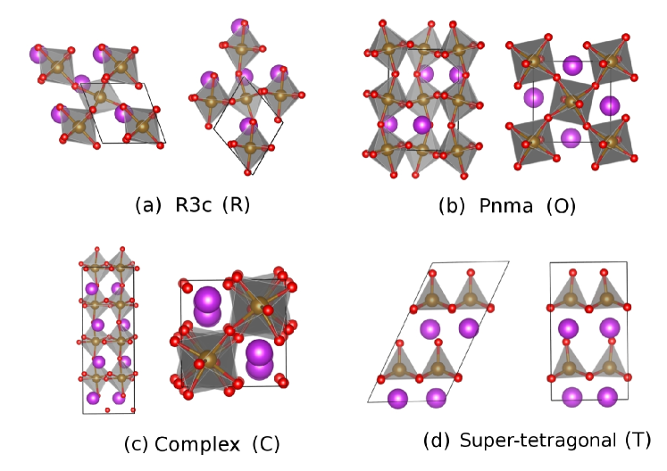
Figure 1: (Color online) Sketch of the four crystal structures considered in this work as seen from two perpendicular directions. Bi, Fe, and O atoms are represented with purple, brown, and red spheres, respectively. Unit cells are depicted with thick solid lines and the O₆ octahedra and O₅ pyramids appear shadowed.

Fortunately, BFO presents a peculiar feature that enormously simplifies the investigation of its phase diagram. Unlike the usual ferroelectric materials, whose transitions are typically driven by the condensation of a soft phonon mode, BFO presents strongly first-order reconstructive transformations between phases that are robustly metastable. This makes it possible to apply to BFO tools that are well-known for the analysis of solid-solid phase transitions in other research fields,cazorla08 ; shevlin12 ; cazorla12 ; cazorla10 ; taioli07 ; cazorla07 ; cazorla09 and which are based on the calculation of the free energy of the individual phases as a function of temperature, pressure, etc. The simplest of such techniques, which requires relatively affordable first-principles simulations, is based on a quasi-harmonic approximation to the calculation of the free energy (QHF method in the following). This is the scheme adopted in this work to investigate BFO’s $p-T$ phase diagram.

We should stress, though, that application of the QHF scheme to BFO is not completely straightforward. Indeed, the spin and vibrational degrees of freedom in multiferroic materials can be expected to couple significantly (i.e., spin-phonon coupling effects become non-negligible,fennie06 ; hee10 ; hemberger06 ; rudolf08 ; hong12 see Fig. 2) implying that the free energies of ferromagnetic, anti-ferromagnetic, and paramagnetic phases belonging to a same crystal structure may differ significantly. The situation becomes especially complicated whenever we have structural transitions involving paramagnetic phases, as capturing the effect of disordered spin arrangements would in principle require the use of very large simulation boxes.kormann08 ; shang10 ; kormann12 In this work we have introduced and applied an approximate scheme to circumvent such a difficulty.

Therefore, here we present a QHF investigation of the $p-T$ phase diagram of BFO, monitoring the relative stability of the four representative phases shown in Fig. 1: the rhombohedral ground state (“${\cal R}$ phase” with $R3c$ space group), the orthorhombic structure that gets stabilized at high temperatures and pressures (“${\cal O}$ phase” with $Pnma$ space group), a phase that is representative of the recently predicted nano-twinned structures displaying complex O₆-rotation patterns (complex or “${\cal C}$ phase”), and the most stable of the super-tetragonal polymorphs that have been predicted to occur in strongly-compressed thin films (“${\cal T}$ phase” with $Cc$ space group). Our calculations take into account the fluctuations of spin ordering in an approximate way and reveal the subtle effects that control the occurrence (or suppression) of all these structures in BFO’s phase diagram.

The organization of this article is as follows. In Section II we provide the technical details of our energy and phonon calculations, and briefly review the fundamentals of the QFH approach. We also explain the strategy that we have followed to effectively cast spin-phonon coupling effects into QHF expressions. In Section III we present and discuss our results. Finally, in Section IV we conclude the article by reviewing our main findings and commenting on prospective work.

II Methods

II.1 First-principles methods

In most of our calculations we used the generalized gradient approximation to density functional theory (DFT) proposed by Perdew, Burke, and Ernzerhof (GGA-PBE),pbe96 as implemented in the VASP package.vasp We worked with GGA-PBE because this is the DFT variant that renders a more accurate description of the relative stability of the ${\cal R}$ and ${\cal O}$ phases of BFO, as discussed in Ref. dieguez11, . A “Hubbard-U” scheme with $U=4$ eV was employed for a better treatment of Fe’s $3d$ electrons. We used the “projector augmented wave” method to represent the ionic cores,bloch94 considering the following electrons as valence states: Fe’s $3s$, $3p$, $3d$, and $4s$; Bi’s $5d$, $6s$, and $6p$; and O’s $2s$ and $2p$. Wave functions were represented in a plane-wave basis truncated at $500$ eV, and each crystal structure was studied on its corresponding unit cell (see Fig. 1). For integrations within the Brillouin zone (BZ), we employed $\Gamma$-centered $k$-point grids whose densities were approximately equivalent to that of a $10\times 10\times 10$ mesh for the ideal cubic perovskite 5-atom cell (e.g., $8\times 8\times 8$ in the ${\cal R}$ phase with $Z=2$, and $6\times 6\times 6$ in the ${\cal O}$ phase with $Z=4$). Using these parameters we obtained energies that were converged to within $0.5$ meV per formula unit (f.u.). Geometry relaxations were performed using a conjugate-gradient algorithm that kept the volume of the unit cell fixed while permitting variations of its shape, and the imposed tolerance on the atomic forces was $0.01$ eV$\cdot$Å^-1. Equilibrium volumes were subsequently determined by fitting the sets of calculated energy points to equations of state. Technical details of our phonon calculations are provided in Secs. II.4 and II.5.

II.2 Quasi-harmonic Free Energy Approach

In the quasi-harmonic approach, one assumes that the potential energy of the crystal can be captured by a quadratic expansion around the equilibrium configuration of the atoms, so that

$$E_{\rm harm}=E_{\rm eq}+\frac{1}{2}\sum_{l\kappa\alpha,l^{\prime}\kappa^{\prime}\alpha^{\prime}}\Phi_{l\kappa\alpha,l^{\prime}\kappa^{\prime}\alpha^{\prime}}u_{l\kappa\alpha}u_{l^{\prime}\kappa^{\prime}\alpha^{\prime}}\;,$$ (1)

where $E_{\rm eq}$ is the total energy of the undistorted lattice, $\bm{\Phi}$ the force-constant matrix, and $u_{l\kappa\alpha}$ is the displacement along Cartesian direction $\alpha$ of the atom $\kappa$ at lattice site $l$. In the usual way, we tackle the associated dynamical problem by introducing

$$u_{l\kappa\alpha}(t)=\sum_{q}u_{q\kappa\alpha}\exp{\left[i\left(\omega t-\bm{q}\cdot(\bm{l}+\bm{\tau}_{\kappa}\right)\right]}\;,$$ (2)

where $\bm{q}$ is a wave vector in the first Brillouin zone (BZ) defined by the equilibrium unit cell; $\bm{l}+\bm{\tau}_{\kappa}$ is the vector that locates the atom $\kappa$ at cell $l$ in the equilibrium structure. Then, the normal modes are found by diagonalizing the dynamical matrix

$$\begin{split}&D_{\bm{q};\kappa\alpha,\kappa^{\prime}\alpha^{\prime}}=\\ &\frac{1}{\sqrt{m_{\kappa}m_{\kappa^{\prime}}}}\sum_{l^{\prime}}\Phi_{0\kappa\alpha,l^{\prime}\kappa^{\prime}\alpha^{\prime}}\exp{\left[i\bm{q}\cdot(\bm{\tau}_{\kappa}-\bm{l^{\prime}}-\bm{\tau}_{\kappa^{\prime}})\right]}\,,\end{split}$$ (3)

and thus treat the material as a collection of non-interacting harmonic oscillators with frequencies $\omega_{\bm{q}s}$ (positively defined and non-zero) and energy levels

$$E^{n}_{\bm{q}s}=\left(\frac{1}{2}+n\right)\omega_{\bm{q}s}\,,$$ (4)

where $0\leq n<\infty$. Within this approximation, the Helmholtz free energy at volume $V$ and temperature $T$ is given by

$$F_{\rm harm}(V,T)=\frac{1}{N_{q}}~{}k_{B}T\sum_{{\bf q}s}\ln\left[2\sinh\left(\frac{\hbar\omega_{{\bf q}s}(V)}{2k_{\rm B}T}\right)\right]\;,$$ (5)

where $N_{q}$ is the total number of wave vectors used in our BZ integration and the dependence of frequencies $\omega_{\bm{q}s}$ on volume is indicated. Finally, the total Helmholtz free energy of the crystal can be written as

$$F_{\rm qh}(V,T)=E_{\rm eq}(V)+F_{\rm harm}(V,T)\;.$$ (6)

We note that the greater contributions to $F_{\rm harm}$ come from the lowest-frequency modes. This implies that, when analyzing the thermodynamic stability of different crystal structures, those which are vibrationally softer in average will benefit more from the dynamical term in $F_{\rm qh}$.

Finally, let us analyze the form that $F_{\rm harm}$ adopts in the limits of low and high temperatures. In the first case, one obtains

$$F_{\rm harm}(V,T\to 0)=\frac{1}{N_{\rm q}}\sum_{\bm{q}s}\frac{1}{2}\hbar\omega_{\bm{q}s}\;;$$ (7)

this result is usually referred to as the zero-point energy (ZPE). As we will see in Sec. III, ZPE corrections may turn out to be decisive in the prediction of accurate transition pressures involving two crystal structures with similar static energies. In the second limiting case, usually termed as the classical limit (i.e., for $\hbar\omega_{\bm{q}s}\ll k_{B}T$), one arrives at the expression

$$F_{\rm harm}(V,T\to\infty)=3N_{\rm uc}k_{B}T\ln\left[\frac{\hbar\bar{\omega}}{k_{B}T}\right]\;.$$ (8)

Here, $N_{\rm uc}$ is the number of atoms in the unit cell, and $\bar{\omega}$ is the geometric average frequency defined as

$$\bar{\omega}=\exp{(\langle\ln\omega\rangle)}\;,$$ (9)

where $\langle\cdots\rangle$ is the arithmetic mean performed over wave-vectors $\bm{q}$ and phonon branches $s$. It is worth noting that low-frequency modes are the ones contributing the most to $\bar{\omega}$, and therefore to $F_{\rm harm}$. As it will be shown in the next section, Eq. (8) allows us to obtain compact and physically insightful expressions for $F_{\rm harm}$ in which spin-phonon coupling effects are effectively accounted for.

Figure 2: Phonon frequency shifts among the ferromagnetic (FM) and G-type anti-ferromagnetic spin arrangements of BFO in the ${\cal R}$ phase, calculated along one representative direction in the first BZ. Corresponding $\omega_{{\bf q}s}$ frequency pairs were identified by comparing the FM and G-AFM phonon eigenmodes.

II.3 Spin-Phonon Couplings

We would like to identify a practical scheme to incorporate the main effects of the spin fluctuations on the calculation of QH Helmholtz free energies. To introduce our approach, let us begin by considering the following general expression for the energy of the material, which is the generalization of Eq. (1) to the case of a compound with localized magnetic moments whose interactions are well captured by a Heisenberg Hamiltonian:

$$\begin{split}E_{\rm harm}(\{u_{m}\},\{S_{i}\})=&E^{0}+\frac{1}{2}\sum_{mn}\Phi_{mn}^{0}u_{m}u_{n}\\ &+\frac{1}{2}\sum_{ij}J_{ij}(\{u_{m}\})S_{i}S_{j}\;,\end{split}$$ (10)

where the $S_{i}$ variables represent the magnetic moments associated with specific atoms and the $J_{ij}$’s are the distortion-dependent exchange interactions coupling them. (For brevity, in the following we will talk about spins instead of magnetic moments; nonetheless, note that our arguments can be applied to cases involving orbital magnetization.) To simplify the notation, we use complex indexes – $m$ and $n$ for the atomic displacements and $i$ and $j$ for the spins – that include information about the cell, atom, and Cartesian component defining the structural and magnetic variables. Finally, we write the dependence of the exchange constants on the atomic displacements as:

$$J_{ij}(\{u_{m}\})=J_{ij}^{(0)}+\sum_{m}J_{ijm}^{(1)}u_{m}+\frac{1}{2}\sum_{mn}J_{ijmn}^{(2)}u_{m}u_{n}\,,$$ (11)

where, for our purposes, it is sufficient to truncate the series at the harmonic level. The $J_{ij}^{(0)}$ parameters describe the magnetic interactions when the atoms remain at their equilibrium positions; typically, these parameters will capture the bulk of the exchange couplings. The $J_{ijm}^{(1)}$ coefficients describe the forces that may appear on the atoms when we have certain spin arrangements, and the $J_{ijmn}^{(2)}$ parameters capture the dependence of the phonon spectrum on the spin configuration.

It is interesting to note that, while the energy in Eq. (1) can be unambiguously described as a harmonic expansion around an equilibrium state of the material, the interpretation of Eq. (10) is much more subtle. Indeed, because we work with spin variables that have a fixed norm (nominally, $|S_{i}|=5\mu_{\rm B}$ in the case of the Fe³⁺ cations in BiFeO₃), the reference structure of our spin-phonon QH energy is defined formally as one in which the atomic spins are perfectly disordered and the atoms are located at the corresponding equilibrium positions. Such a structure cannot be easily considered in a first-principles calculation; hence, we have to obtain the parameters $E^{0}$ and $\Phi_{mn}^{0}$ that characterize it in an indirect way. In essence, the fitting procedure would involve many different spin configurations, and parameters $E^{0}$ and $\Phi_{mn}^{0}$ would capture the part of the energy and force-constant matrix that is independent of the spin order. Further, a thorough calculation of the $J_{ij}(\{u_{m}\})$ constants would be a very challenging task. Indeed, a detailed modeling of the spin-phonon couplings would require us to choose which spin pairs $i$ and $j$ are affected by which distortions pairs $m$ and $n$, a problem that quickly grows in complexity even if we restrict ourselves to spin interactions between first nearest neighbors.

In this work we did not attempt to pursue such a detailed description, but adopted instead an approximate approach that provides the correct results in particular important cases. To illustrate our scheme, let us think of BFO’s ${\cal R}$ phase and consider two specific spin arrangements that are obviously relevant: (1) the G-AFM structure (which is the ground state of the ${\cal R}$, ${\cal O}$, and ${\cal C}$ BFO phases mentioned above) and (2) a perfectly ferromagnetic (FM) arrangement, which is the exact opposite case to G-AFM in the sense that all the interactions between first nearest-neighboring spins are reversed. Let us also restrict ourselves to spin-spin interactions between first nearest neighbors and, for the sake of simplicity, let us assume that all first-nearest-neighboring spins are coupled by the same $J$, so that we can drop the $i$ and $j$ indexes. (This is actually the case for the ${\cal R}$ phase of BFO, and the generalization to other lower-symmetry cases is straightforward.) Then, for a given spin arrangement $\gamma$ (where $\gamma$ can be G-AFM or FM in this example), we can relax the atomic structure of the material and construct the following energy $E^{\gamma}_{\rm harm}$

$$E_{\rm harm}^{\gamma}(\{u_{m}\})=E_{\rm eq}^{\gamma}+\frac{1}{2}\sum_{mn}\Phi^{\gamma}_{mn}u_{m}u_{n}\;,$$ (12)

which is the analogous of Eq. (1) above. Hence, we have straightforward access to all the parameters in this expression from first principles. Now, we want our general spin-phonon energy in Eq. (10) to reproduce $E^{\gamma}_{\rm harm}$ for the $\gamma$-orders of interest. If we are dealing with the G-AFM and FM cases, it is trivial to check that this can be achieved by making the following choices:

$$E^{0}=\frac{1}{2}\left(E^{\rm FM}_{\rm eq}+E^{\rm G}_{\rm eq}\right)\,,$$ (13)

$$\Phi_{mn}^{0}=\frac{1}{2}\left(\Phi_{mn}^{{\rm FM}}+\Phi_{mn}^{{\rm G}}\right)\,,$$ (14)

$$J^{(0)}=\frac{1}{6|S|^{2}}\left(E^{\rm FM}_{\rm eq}-E^{\rm G}_{\rm eq}\right)\,,$$ (15)

$$J^{(1)}_{m}=0\,,$$ (16)

$$J^{(2)}_{mn}=\frac{1}{6|S|^{2}}\left(\Phi_{mn}^{{\rm FM}}-\Phi_{mn}^{{\rm G}}\right)\,.$$ (17)

While these choices may seem very natural, there are subtle approximations and simplifications hiding behind them. For example, the resulting model contains no explicit information about the atomic rearrangements that may accompany a particular spin configuration; nevertheless, the energies of the equilibrium structures are perfectly well reproduced for the G-AFM and FM cases. Analogously, while the phonons of the G-AFM and FM cases will be exactly reproduced by this model, the spin-phonon interactions have been drastically simplified, and we retain no information on how specific atomic motions affect specific exchange constants. Hence, the resulting model should not be viewed as an atomistic one; rather, it is closer to a phenomenological approach in which we retain information about the effect of magnetic order on the whole phonon spectrum.

Finally, we would like to use our spin-phonon energy to investigate the properties of BFO at finite temperatures, especially in situations in which the material is either paramagnetic (PM) or does not have a fully developed AFM order. To do so, we will assume that, for the case of fluctuating spins, the energetics of the atomic distortions is approximately given by:

$$\begin{split}\tilde{E}_{\rm harm}(\{u_{m}\};x)&=E^{0}+3x|S|^{2}J^{(0)}\\ &+\frac{1}{2}\sum_{mn}\left(\Phi_{mn}^{0}+6x|S|^{2}J^{(2)}_{mn}\right)u_{m}u_{n}\,,\end{split}$$ (18)

where $x=\langle S_{i}S_{j}\rangle/|S|^{2}$ is the correlation function between two neighboring spins, with $\langle...\rangle$ indicating a thermal average. Note that in the limiting FM ($\langle S_{i}S_{j}\rangle=|S|^{2}$) and G-AFM ($\langle S_{i}S_{j}\rangle=-|S|^{2}$) cases, this equation reduces to the expected $E^{\rm FM}_{\rm harm}$ and $E^{\rm G}_{\rm harm}$ energies. Note also that this model includes a spin-phonon contribution to the energy even in the paramagnetic phase, as long as there are significant correlations between neighboring spins. Indeed, for a non-zero value of $x$, the phonon spectrum is given by the force-constant matrix $\bm{\Xi}(x)\equiv\bm{\Phi}^{0}+6x|S|^{2}\bm{J}^{(2)}$.

In this work, we evaluate $x$ as a function of temperature by running Monte Carlo simulations of the Heisenberg spin system described by the $J^{(0)}_{ij}$ coupling constants, thus assuming frozen atomic distortions. Then, since for a certain value of $x$ Eq. (18) is formally analogous to Eq. (1), we can apply the QH treatment described above to estimate the Helmholtz free energy $\tilde{F}_{\rm harm}$ of the coupled spin-phonon system.

Before concluding this section, let us discuss some approximate expressions that can be obtained for $\tilde{F}_{\rm harm}$ and which are illustrative of how our approach captures the effect of spin fluctuations and of the peculiar nature of the paramagnetic state. We have usually observed that the normal-mode frequencies $\omega_{\bm{q}s}^{\gamma}$, obtained by diagonalizing the dynamical matrix associated to $\bm{\Phi}^{\gamma}$, depend significantly on the magnetic order. However, the corresponding eigenvectors are largely independent from $\gamma$. As a result we have the following approximate relations

$$\tilde{\omega}_{{\bf q}s}\approx\omega_{{\bf q}s}^{\rm FM}\sqrt{\left(\frac{\omega_{{\bf q}s}^{\rm G}}{\omega_{{\bf q}s}^{\rm FM}}\right)^{2}\left(\frac{1-x}{2}\right)+\left(\frac{1+x}{2}\right)}=$$

$$\omega_{{\bf q}s}^{\rm G}\sqrt{\left(\frac{1-x}{2}\right)+\left(\frac{\omega_{{\bf q}s}^{\rm FM}}{\omega_{{\bf q}s}^{\rm G}}\right)^{2}\left(\frac{1+x}{2}\right)}\,,$$ (19)

where $\{\tilde{\omega}_{\bm{q}s}\}$ are the frequencies associated to $\bm{\Xi}(x)$. Using this result, we can write the Helmholtz free energy in the high temperature limit as

$$\tilde{F}_{\rm harm}(V,T\to\infty,\{{\bf S}\})=\left(\frac{F_{\rm harm}^{\rm FM}+F_{\rm harm}^{\rm G}}{2}\right)+$$

$$\frac{3}{2}Nk_{B}T\sum_{{\bf q},s}{\rm ln}\left[\frac{\left(\omega_{{\bf q}s}^{\rm FM}\right)^{2}\left(1+x\right)+\left(\omega_{{\bf q}s}^{\rm G}\right)^{2}\left(1-x\right)}{2\omega_{{\bf q}s}^{\rm FM}\cdot\omega_{{\bf q}s}^{\rm G}}\right]$$ (20)

where terms $F_{\rm harm}^{\rm FM}$ and $F_{\rm harm}^{\rm G}$ are calculated in the classical limit through Eq. (8) and correspond to perfect FM and G-AFM spin arrangements. Note that in the limiting cases $x=1$ and $x=-1$, Eq. (20) consistently reduces to $F_{\rm harm}^{\rm FM}$ and $F_{\rm harm}^{\rm G}$. Interestingly, in the ideal paramagnetic case $x=0$ we find that, since all $\omega_{{\bf q}s}$ are positive, the inequality $\tilde{F}_{\rm harm}>\frac{1}{2}\left(F_{\rm harm}^{\rm FM}+F_{\rm harm}^{\rm G}\right)$ holds. This result sets a lower bound for the error that we would be making if the spin disorder in ideal paramagnetic phases was neglected. For example, in the case of the ${\cal R}$ phase of BFO, if we used a frozen G-AFM spin structure in our QH calculations, the resulting free energy error would be of order $\frac{1}{2}\left(F_{\rm harm}^{\rm FM}-F_{\rm harm}^{\rm G}\right)$.

II.4 Phonon Calculations

In order to compute the QH free energy of a crystal, it is necessary to know its full phonon spectrum over the whole BZ. There are essentially two methods which can be used for the calculation of the phonon frequencies: linear response theory and the direct approach. The first method is generally exploited within the framework of density functional perturbation theory (DFPT);baroni87 ; baroni01 ; gonze89 ; gonze97 the main idea in DFPT is that a linear order variation in the electron density upon application of a perturbation to the crystal is the responsible for the variation in the energy up to third order in the perturbation. If the perturbation is a phonon wave with wave-vector ${\bf q}$, the calculation of the density change to linear order can thus be used to determine the dynamical matrix at wave-vector ${\bf q}$. This procedure can be repeated at any wave-vector and without the need to construct a supercell. In the direct approach, in contrast, the force-constant matrix is directly calculated in real-space by considering the proportionality between the atomic displacements and forces when the former are sufficiently small (see Sec. II.2).kresse95 ; alfe01 In this case, large supercells have to be constructed in order to guarantee that the elements of the force-constant matrix have all fallen off to negligible values at their boundaries, a condition that follows from the use of periodic boundary conditions.alfe09 Once the force-constant matrix is thus obtained, we can Fourier-transform it to obtain the phonon spectrum at any $q$-point. In this work we chose to perform phonon frequencies calculations with the direct method. Nevertheless, convergence of the force-constant matrix elements with respect to the size of the supercell in polar materials may be slow due to the appearance of charge dipoles and macroscopic electric fields in the limit of zero wave-vector; in the next section we explain how we have efficiently dealt with this issue.

We performed a series of initial tests in the ${\cal R}$ phase to determine the value of the various calculation parameters that guarantee $F_{\rm harm}$ results converged to within $5$ meV/f.u. (As it will be shown later, this accuracy threshold translates into uncertainties of about 100 K in the predicted transition temperatures.) The quantities with respect to which our QH free energies need to be converged are the size of the supercell, the size of the atomic displacements, and the numerical accuracy in the calculation of the atomic forces and BZ sampling (see Eq. 5). We found the following settings to fulfill our convergence requirements: $2\times 2\times 2$ supercells (i.e., 8 replications of the 10-atom unit cell of the ${\cal R}$ phase), atomic displacements of $0.02$ Å, and special Monkhorst-Packmonkhorst76 grids of $12\times 12\times 12$ $q$-points, corresponding to the BZ of the ${\cal R}$-phase unit cell, to compute the sums in Eq. (5). Regarding the calculation of the atomic forces with VASP, we found that the density of $k$-points for BZ integrations had to be increased slightly with respect to the value used in the energy calculations (e.g., from $8\times 8\times 8$ to $10\times 10\times 10$ for the BZ of the unit cell of the ${\cal R}$ phase) and that computation of the non-local parts of the pseudopotential contributions had to be performed in reciprocal, rather than real, space. These technicalities were adopted in all the phonon calculations, adapting in each crystal structure to the appropriate $q$- and $k$-point densities. The value of the phonon frequencies and quasi-harmonic free energies were obtained with the PHON code developed by Alfè.alfe09 ; phon In using this code, we exploited the translational invariance of the system to impose the three acoustic branches to be exactly zero at the $\Gamma$ $q$-point, and used central differences in the atomic forces (i.e., we considered positive and negative atomic displacements). As an example of our phonon frequency calculations, we show in Fig. 3 the full phonon spectrum obtained for the ${\cal R}$ phase of BFO with a G-AFM spin arrangement at zero pressure and when accounting for long-range dipole-dipole interactions as described in the next section.

II.5 Treatment of long-range Coulomb forces

As noted in the previous section, the displacement of atoms in an insulator like BFO creates electric dipoles and long-range dipole-dipole interactions; as a consequence, the interatomic force constants $\Phi_{mn}$ decay typically with the third power of the interatomic distance. These long-range interactions play a critical role in determining the spectrum of long-wavelength phonons. In the direct approach, the phonon frequencies are exactly calculated at wave-vectors ${\bf q}$ that are commensurable with the supercell; thus, unaffordably large simulation boxes would in principle be needed to accurately describe long-wavelength phonons.

Nevertheless, the long-range dipole-dipole interactions can be modeled at the harmonic level from knowledge of the atomic Born effective charge tensors and the dielectric tensor of the material.gonze97 ; cochran62 Taking advantage of such a result, Wang et al. proposed a mixed-space approach in which accurate force constants $\bm{\Phi}$ are calculated with the direct approach in real space and long-range dipole-dipole interactions with linear response theory in reciprocal space.wang10 Wang’s approach is based on the ad hoc inclusion of a long-range force-constant matrix of the form

$$\varphi_{l\kappa\alpha,l^{\prime}\kappa^{\prime}\alpha^{\prime}}=\frac{4\pi e^{2}}{NV}\frac{\left(\sum_{\beta}q_{\beta}Z^{*}_{\kappa\beta,\alpha}\right)\left(\sum_{\beta}q_{\beta}Z^{*}_{\kappa\beta,\alpha^{\prime}}\right)}{\sum_{\beta\beta^{\prime}}q_{\beta}\epsilon^{\infty}_{\beta\beta^{\prime}}q_{\beta^{\prime}}}$$ (21)

where $N$ is the number of primitive cells in the supercell and $V$ its volume; $e$ is the elemental charge, $\bm{\epsilon}^{\infty}$ is the electronic dielectric tensor, and $Z^{*}_{\kappa\beta,\alpha}$ is the Born effective charge quantifying the polarization created along Cartesian direction $\alpha$ when atom $\kappa$ moves along $\beta$. It can be shown that, by Fourier-transforming the modified force-constant matrix $\bm{\Omega}=\bm{\Phi}+\bm{\varphi}$, one obtains the correct behavior near the $\Gamma$ point; further, for ${\bf q}\neq 0$ wave vectors one obtains a smooth interpolation that recovers the exact results at the $q$-points commensurate with the supercell employed for the calculation of $\bm{\Phi}$.wang10

In Table I and Fig. 3, we report the phonon frequencies that we have obtained for the ${\cal R}$ phase of BFO using Wang’s mixed-space approach, and compare them to previous experimental and theoretical data found in Refs. hlinka11, ; borissenko13, ; hermet07, . As it may be appreciated there, the agreement between our $\Gamma$-phonon results and the measurements is very good, indeed comparable to that achieved with DFPT calculations performed by other authors. (Actually, Wang’s method has already been applied with success to the study of the phonon dispersion curves and the heat capacity of BFO.wang11 ) After checking the numerical accuracy of Wang’s technique, we performed a test in which we assessed the $F_{\rm qh}$ differences obtained by using the original and mixed-space versions of the direct approach. We found that the effect of considering long-range dipole-dipole interactions in the QH energies was to vary $F_{\rm qh}$ in less than $5$ meV/f.u., which is our targeted accuracy threshold. In view of the small size of these corrections, and for the sake of computational affordability, we decided not to consider $\bm{\varphi}$ terms in our subsequent calculations, for which we just employed the original real-space version of the direct approach. In fact, as it has already been pointed out by Alfè,alfe09 in the typical case an incorrect treatment of the longitudinal optical modes near the $\Gamma$-point compromises only a small region of the BZ, and the resulting errors in the free energy are small and can in principle be neglected.

$\quad{\rm TO~{}modes}\quad$	$\quad{\rm This~{}work}\quad$	$\quad{\rm Expt.}\quad$	$\quad{\rm Calc.}\quad$	$\quad{\rm LO~{}modes}\quad$	$\quad{\rm This~{}work}\quad$	$\quad{\rm Expt.}\quad$	$\quad{\rm Calc.}\quad$
$E({\rm TO1})$	$78$	$74$	$102$	$E({\rm LO1})$	$85$	$81$	$104$
$E({\rm TO2})$	$136$	$132$	$152$	$E({\rm LO2})$	$161$	$175$	$175$
$E({\rm TO3})$	$238$	$240$	$237$	$E({\rm LO3})$	$242$	$242$	$237$
$E({\rm TO4})$	$252$	$265$	$263$	$E({\rm LO4})$	$258$	$276$	$264$
$E({\rm TO5})$	$265$	$278$	$274$	$E({\rm LO5})$	$323$	$346$	$332$
$E({\rm TO6})$	$330$	$351$	$335$	$E({\rm LO6})$	$352$	$368$	$377$
$E({\rm TO7})$	$361$	$374$	$378$	$E({\rm LO7})$	$393$	$430$	$386$
$E({\rm TO8})$	$412$	$441$	$409$	$E({\rm LO8})$	$445$	$468$	$436$
$E({\rm TO9})$	$488$	$523$	$509$	$E({\rm LO9})$	$483$	$616$	$547$
$A_{1}({\rm TO1})$	$151$	$149$	$167$	$A_{1}({\rm LO1})$	$172$	$178$	$180$
$A_{1}({\rm TO2})$	$219$	$223$	$266$	$A_{1}({\rm LO2})$	$240$	$229$	$277$
$A_{1}({\rm TO3})$	$285$	$310$	$318$	$A_{1}({\rm LO3})$	$461$	$502$	$428$
$A_{1}({\rm TO4})$	$506$	$557$	$517$	$A_{1}({\rm LO4})$	$550$	$591$	$535$
				$A_{2}({\rm LO1})$	$101$	$109$	$109$

Table 1: $\Gamma$-point phonon frequencies of the ${\cal R}$ phase of BFO with G-AFM spin order, calculated using the direct approach and considering long-range dipole-dipole interactions. Experimental values are taken from Refs. hlinka11, and borissenko13, , and previous LSDA-DFPT calculations from Ref. hermet07, . Frequencies are expressed in units of cm^-1.

Figure 3: Phonon spectrum of the ${\cal R}$ phase of BFO with G-AFM spin order, calculated with the direct approach and considering long-range dipole-dipole interactions. The corresponding equilibrium volume per formula unit is 64.35 Å³.

III Results and Discussion

III.1 Stability of the ${\cal R}$ and ${\cal O}$ phases at constant-volume and frozen-spin conditions

Figure 4: Quasi-harmonic free energies of the ${\cal R}$ and ${\cal O}$ phases of BFO, calculated at $p\approx 0$ GPa (i.e., neglecting $T$-induced volume expansion effects) and considering a perfect G-AFM spin order in both structures. The size of the ZPE corrections is shown in the vertical axis. Inset: Plot of the quasi-harmonic free energy difference $\Delta F_{\rm qh}\equiv F_{\rm qh}({\cal R})-F_{\rm qh}({\cal O})$ expressed as a function of temperature.

In this section, we present our QH results for the ${\cal R}$ and ${\cal O}$ phases of BFO. For the sake of clarity, we first discuss the results obtained when spin-disorder and volume-expansion effects are neglected.

In Fig. 4 we plot the $F_{\rm qh}$ energy of the ${\cal R}$ and ${\cal O}$ phases calculated at $p\approx 0$ GPa as a function of temperature. Volumes were kept fixed at their equilibrium values $V_{0}$ obtained at $T=0$ K, which are equal to 64.61 Å³/f.u. and 61.99 Å³/f.u., respectively. We considered the perfect G-AFM spin order to be frozen in both structures. We computed $F_{\rm qh}$ over sets of fourteen temperature points taken at intervals of 100 K and fitted them to third-order polynomial curves. ZPE corrections (see Eq. 7) were included in the fits and are equal to 0.263(5) eV/f.u. and 0.248(5) eV/f.u., respectively, for the ${\cal R}$ and ${\cal O}$ phases. (An estimate of the error is given within parentheses.) We find that at $T=0$ K the ${\cal R}$ phase is energetically more favorable than the ${\cal O}$ phase by 0.046(5) eV/f.u. As the temperature is raised, however, the Helmholtz free energy of the ${\cal O}$ phase becomes lower than that of the ${\cal R}$ phase due to the increasingly more favorable $F_{\rm harm}$ contributions. For instance, at $T=300$ K, $F_{\rm harm}$ amounts to 0.048(5) eV/f.u. for the ${\cal O}$ phase and 0.077(5) eV/f.u. for the ${\cal R}$ phase, whereas at $T=1000$ K the obtained values are $-$1.481(5) eV/f.u. and $-$1.414(5) eV/f.u., respectively. Consequently, a first-order phase transition of the ${\cal R}\to{\cal O}$ type is predicted to occur at $T_{t}$ = 900(100) K. We show this in the inset of Fig. 4, where the energy difference $\Delta F_{\rm qh}\equiv F_{\rm qh}({\cal R})-F_{\rm qh}({\cal O})$ is represented as a function of temperature; since quasi-equilibrium conditions are assumed, the corresponding transition temperature coincides with the point at which $\Delta F_{\rm qh}=0$. We notice that this estimation of $T_{t}$ is reasonably close to the experimental value of 1100 K.arnold09 ; catalan09

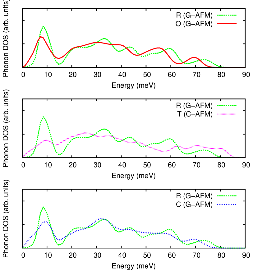
Figure 5: (Color online) Phonon density of states of various BFO phases obtained at $p=0$ GPa. The corresponding equilibrium volumes are 64.61 Å³/f.u., 61.99 Å³/f.u., 71.12 Å³/f.u., and 64.17 Å³/f.u. for the ${\cal R}$, ${\cal O}$, ${\cal T}$, and ${\cal C}$ phases, respectively.

Let us now discuss the origin of the obtained solid-solid transformation in terms of the phonon eigenmodes and frequencies of each phase. In Fig. 5 we plot the phonon density of states (pDOS) calculated for the ${\cal R}$ and ${\cal O}$ phases at their equilibrium volumes. We find that the value of the geometric frequency $\bar{\omega}$ (see Eq. 9) is 27.16 meV in the ${\cal O}$ phase and 28.58 meV in the ${\cal R}$ structure (expressed in units of $\hbar$). Therefore, as it was already expected from the results shown in Fig. 4, the ${\cal O}$ phase of BFO is, in average, vibrationally softer than the ${\cal R}$ phase. In particular, the pDOS of the ${\cal O}$ phase accumulates a larger number of phonon modes within the low-energy region of the spectrum, and extends over a smaller range of frequencies.

We restrict our following analysis to the low-energy phonons (i.e., $\omega_{{\bf q}s}\leq\bar{\omega}$), which provide the dominant contributions to $F_{\rm harm}$. In the ${\cal R}$ phase, we observe a sharp pDOS peak centered at $\hbar\omega\sim 10$ meV followed by a deep valley. By inspecting the spectrum of phonon eigenmodes obtained at $\Gamma$ and the full phonon bands displayed in Fig. 3, we identify that pDOS maximum with the first optical transverse mode TO1 (see Fig. 6). This phonon mode involves opposed displacements of neighboring Bi atoms within the plane perpendicular to the pseudo-cubic direction $[111]$, and is polar in the $[10\bar{1}]$ direction.aclaration-polarity Figure 7 gives additional information on the three lowest-lying phonons of the ${\cal R}$ phase across the BZ. There we can see that the softest phonons are acoustic in character and correspond to $q$-points in the neighborhood of $\Gamma$. As we move away from $\Gamma$, the lowest-lying phonon modes change of character and can be represented by the optical distortion shown in Fig. 6.

The situation for the ${\cal O}$ phase is rather different. As it can be appreciated from Fig. 5, the number of phonons in the very low-frequency region is much greater than in the ${\cal R}$ phase. Small frequency values are in general related to phonon modes of strong acoustic character, which are the responsible for the elastic response of materials: the softer a crystal is, the smaller the slopes of its acoustic bands around the $\Gamma$ $q$-point, and the larger the number of low-energy phonons that result. By applying this reasoning to the present case and considering our pDOS results, one would arrive at the conclusion that BFO in the ${\cal O}$ phase should be elastically softer than in the ${\cal R}$ phase. However, this is not the case: we computed the equilibrium bulk modulus of BFO (i.e., $B\equiv-V\frac{\partial p}{\partial V}$) at $T=0$ K describing the response of the material to uniform deformations and found, respectively, $99(2)$ GPa and $158(2)$ GPa for the ${\cal R}$ and ${\cal O}$ structures. Interestingly, this apparent contradiction is quickly resolved by inspecting the behavior of the (three) lowest-lying phonons calculated at each BZ $q$-point (see Fig. 8). As clearly observed in Fig. 8, the ${\cal O}$ phase of BFO presents very low-lying optical bands with phonon frequencies that can be below 2 meV. The corresponding eigenmodes are dominated by the stretching of Bi–O bonds, with the Fe ions having a very minor contribution (see middle panel in Fig. 8). In fact, these soft optical phonons, with ${\bf q}$ vectors far away from $\Gamma$, are the ones responsible for the stabilization of BFO’s ${\cal O}$ phase at high temperatures.

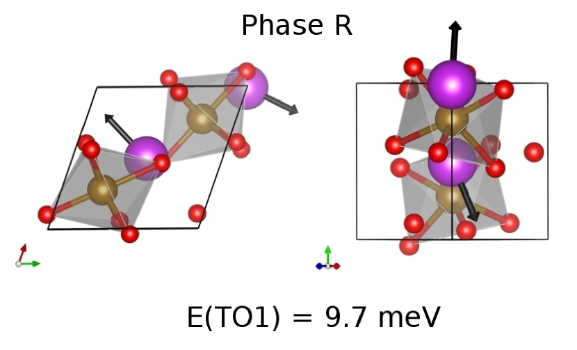
Figure 6: (Color online) Sketch of the first optical transverse $\Gamma$-point phonon mode obtained in the ${\cal R}$ phase of BFO at equilibrium. Bi displacements are represented with black arrows, and Bi, Fe, and O atoms with purple, brown and red spheres, respectively.

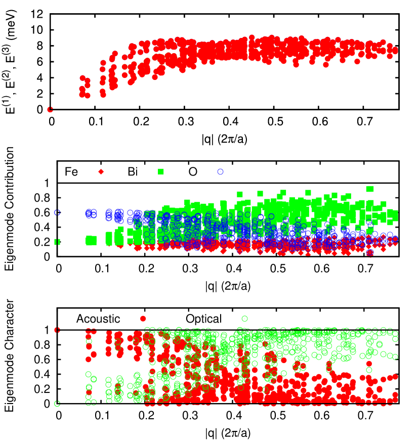
Figure 7: (Color online) Analysis of the three lowest-energy phonon eigenmodes obtained at the $q$-points used for the sampling of the BZ of BFO’s ${\cal R}$ phase. We represent their eigenenergies as a function of wave-vector module in the top panel, the contribution of each atomic species to the mode eigenvectors in the middle panel, and a quantification of their acoustic and optical characters in the bottom panel. For this quantification, we took advantage of the normalization and orthogonality relations satisfied by the eigenvectors of the dynamical matrix calculated at $\Gamma$ and ${\bf q}\neq 0$ points.

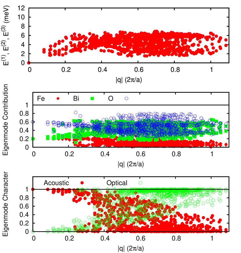
Figure 8: (Color online) Same as Fig. 7, but for BFO’s ${\cal O}$ phase.

III.2 Effect of spin disorder on the ${\cal R}\to{\cal O}$ transition

Figure 9: Monte Carlo results obtained for a simple Heisenberg model reproducing the spin magnetic order in the ${\cal R}$ and ${\cal O}$ phases of BFO. Top: Average value of the normalized spin product ${\bf S}_{i}\cdot{\bf S}_{j}$ (with $S\equiv 5/2\mu_{\rm B}$) as a function of temperature. Bottom: Calculated order parameter $S_{\rm G}$ (see text) as a function of temperature.

Figure 10: Quasi-harmonic free energy difference between the ${\cal R}$ and ${\cal O}$ phases of BFO. We show the results obtained in two different situations, i.e., frozen G-AFM and $T$-dependent spin orders (solid symbols and error bars correspond to the last case). Lines are linear fits to the free energy results.

In order to assess the effect of spin fluctuations on the predicted ${\cal R}\to{\cal O}$ phase transition, we put in practice the ideas explained in Sec. II.3. As described there, our practical approach to capture the effects of spin disorder requires the calculation of the QH energies for the G-AFM ($F_{\rm qh}^{\rm G}$; this is the case already considered in the previous section) and FM ($F_{\rm qh}^{\rm FM}$) spin arrangements, from which we derive the parameters describing (1) the spin-independent part of the energy ($E^{0}$ and $\bm{\Phi}^{0}$), (2) the Heisenberg spin Hamiltonian for zero atomic distortions ($J^{0}$), and (3) the effects of the spin arrangement on the phonon spectrum ($\bm{J}^{(2)}$). Our DFT calculations render $J^{(0)}$ values of 34.67 meV and 32.67 meV, respectively, for the ${\cal R}$ and ${\cal O}$ phases, indicating a similar and strong tendency towards the G-AFM order. Further, Fig. 2 shows illustrative results of the shifts in phonon frequencies, for the ${\cal R}$ phase of BFO, that occur as a function of the spin structure; these are the effects captured by the $\bm{J}^{(2)}$ terms.

Figure 9 reports the results of a series of Monte Carlo (MC) simulations performed with the Heisenberg model defined by the $J^{(0)}$ coupling. We used a periodically-repeated simulation box of $20\times 20\times 20$ spins, and computed the thermal averages from runs of 50000 MC sweeps. The aim of these simulations was to determine the value of the spin average $\langle{\bf S}_{i}\cdot{\bf S}_{j}\rangle$ that has to be used in Eqs. (18)-(19) and which depends on $T$. Note that here we have abandoned the compact notation of Section II.3, and $S_{i\alpha}$ denotes the $\alpha$ Cartesian component of the spin at cell $i$. Additionally, these simulations allow us to monitor the occurrence of magnetic transitions through the computation of the G-AFM order parameter $S^{\rm G}=\frac{1}{N}\sum_{i}(-1)^{n_{ix}+n_{iy}+n_{iz}}S_{iz}$. Here, $n_{ix}$, $n_{iy}$, and $n_{iz}$ are the three integers locating the $i$-th lattice cell, and $N$ is the total number of spins in the simulation box; further, for the calculation of $S^{\rm G}$, we need to consider only the $z$ component of the spins because of a small symmetry-breaking magnetic anisotropy that was included in our Hamiltonian to facilitate the analysis (see Supplemental Material of Ref. escorihuela12, ). Our results show that in the ${\cal R}$ phase the magnetic phase transition occurs at $T\sim 600$ K, a temperature that is rather close to the experimental value $T_{N}\sim 650$ K.kiselev63 ; smolenskii61 ; catalan09 The results for the ${\cal O}$ phase are very similar.

Now, let us assess the consequences of considering these effects on the QH free energies of the ${\cal R}$ and ${\cal O}$ phases (see Eqs. 18-19). Figure 10 reports the free energy difference between the ${\cal R}$ and ${\cal O}$ phases, as obtained by considering ($\Delta\tilde{F}_{\rm qh}$) or neglecting ($\Delta F_{\rm qh}$) the effect of the spin fluctuations. As one can appreciate, the two curves are almost identical and provide the same transition temperature. At $T=300$ K, for instance, both $\Delta F^{\rm G}_{\rm qh}$ and $\Delta\tilde{F}_{\rm qh}$ are about $-$0.032(5) eV/f.u., and at $T=1000$ K we get approximately 0.006(5) eV/f.u.; that is, the differences fall within the accuracy threshold set in our free energy calculations.

However, the consequences of considering $T$-dependent spin arrangements in the calculation of the QH free energy of an individual phase are actually quite sizable. Indeed, the error function defined as $\delta\tilde{F}_{\rm qh}\equiv\tilde{F}_{\rm qh}-F^{\rm G}_{\rm qh}$ may amount to several tenths of eV at high temperatures. For instance, for the ${\cal R}$ phase, $\delta\tilde{F}_{\rm qh}$ is 0.068(5) eV/f.u. at $T=300$ K and 0.102(5) eV/f.u. at $T=1000$ K. Hence, the reason behind the numerical equivalence between functions $\Delta F^{\rm G}_{\rm qh}$ and $\Delta\tilde{F}_{\rm qh}$ is that $\delta\tilde{F}_{\rm qh}$ errors are essentially the same in both ${\cal R}$ and ${\cal O}$ structures and thus they cancel. Consequently, it is possible to obtain reasonable $T_{t}$ predictions in BFO even if one neglects the strong dependence of spin magnetic order on temperature.

In view of this conclusion, and for the sake of computational affordability, we will disregard spin-disorder effects for the rest of phases considered in this work. Also, we note that the inequality $\tilde{F}_{\rm harm}>\frac{1}{2}\left(F_{\rm harm}^{\rm FM}+F_{\rm harm}^{\rm G}\right)$, mentioned in Sec. II.3, is fulfilled for both the ${\cal R}$ and ${\cal O}$ structures at all temperatures, even when $x=\langle{\bf S}_{i}\cdot{\bf S}_{j}\rangle/|S|^{2}\neq 0$ and $\hbar\bar{\omega}\approx k_{B}T$. Plausibly then, the lower bound set there for the QH errors caused by neglecting the spin disorder can be tentatively generalized to any value of $x$.

Figure 11: Calculated two-phase boundary delimiting the ${\cal R}$ and ${\cal O}$ regions in the bulk phase diagram of BFO at elevated temperatures. The solid line is a guide to the eyes and the symbols represent explicitly calculated points. Inset: $E_{\rm eq}$ curves obtained for the ${\cal R}$ and ${\cal O}$ phases as a function of volume without considering ZPE corrections.

Figure 12: Quasi-harmonic free energy differences among the ${\cal R}$ phase and the rest of crystal structures analyzed in this work. Perfect G-AFM spin order and constrained equilibrium volumes were considered. Lines are guides to the eyes and the symbols represent explicitly calculated points.

III.3 Effect of volume expansion on the ${\cal R}\to{\cal O}$ transition

To address the effect of volume expansion on $T_{t}$, we performed additional energy, phonon, and $F_{\rm qh}$ calculations over a grid of five volumes spanning the interval $0.95\leq V/V_{0}\leq 1.10$ for both ${\cal R}$ and ${\cal O}$ phases. At each volume, first we computed the value of $F_{\rm qh}$ at a series of temperatures in the range between 0 K and 1600 K, taken at $100$ K intervals. Then, at each $T$ we fitted the corresponding $F_{\rm qh}(V,T)$ points to third-order Birch-Murnaghan equationsbirch78 ; cazorla13 and performed Maxwell double-tangent constructions over the resulting ${\cal R}$ and ${\cal O}$ curves to determine $p_{t}(T)$ (i.e., the pressure at which the first-order ${\cal R}\to{\cal O}$ transition occurs at a given $T$). By repeating this process several times we were able to draw the ${\cal R}$–${\cal O}$ phase boundary, $p_{t}(T)$, in the interval $-$0.1 GPa $\leq p\leq 0.6$ GPa. Figure 11 reports these results. As one can appreciate there, the calculated transition temperature at equilibrium now is 1300(100) K. Volume expansion effects, therefore, shift upwards by 400 K our previous tentative $T_{t}$ estimation. Also, we find that the volume of the crystal varies from 66.51 Å³/f.u. to 62.34 Å³/f.u. during the course of the ${\cal R}\to{\cal O}$ transformation. These values can be compared to recent experimental data obtained by Arnold et al.arnold09 which are $T_{\rm C}\approx 1100$ K, $V({\cal R})=64.15$ Å³/f.u. and $V({\cal O})=63.10$ Å³/f.u. In general, our agreement with respect to Arnold’s measurements can be regarded as reasonably good, although our QH calculations overestimate the transition temperature and volume reduction $\Delta V=V({\cal O})-V({\cal R})$ observed in experiments.

Moreover, in the vicinity of the transition state [0 GPa, 1300(100) K], we assumed the slope of the phase boundary to be constant and numerically computed $dT/dp\approx-$1100 K/GPa. By introducing this value and $\Delta V=-$4.17 Å³/f.u. in the Clausius-Clapeyron equation, we found the latent heat of the ferroelectric phase transformation to be about 0.71 Kcal/mol. Unfortunately, we do not know of any experimental data to compare this result with. Interestingly, if we assume the slope of the ${\cal R}$–${\cal O}$ phase boundary to be constant regardless of the $p-T$ conditions, the extrapolated zero-temperature ${\cal R}\to{\cal O}$ transition turns out to be $p_{t}(0)\sim 1.2$ GPa. This result differs greatly from the $p_{t}(0~{}K)$ value obtained when straightforwardly considering static $E_{\rm eq}$ curves (see inset of Fig. 11) and enthalpies (i.e., $H_{\rm eq}=E_{\rm eq}+p_{\rm eq}V$), which is 4.8 GPa. This disagreement may indicate that assuming global linear behavior in $p_{t}(T)$ is unrealistic and/or that ZPE corrections in BFO are very important. We will comment again on this point in Sec. III.6, when analyzing in detail the role of ZPE corrections in prediction of $p$-induced phase transformations at $T=0$ K.

III.4 The complex ${\cal C}$ phase

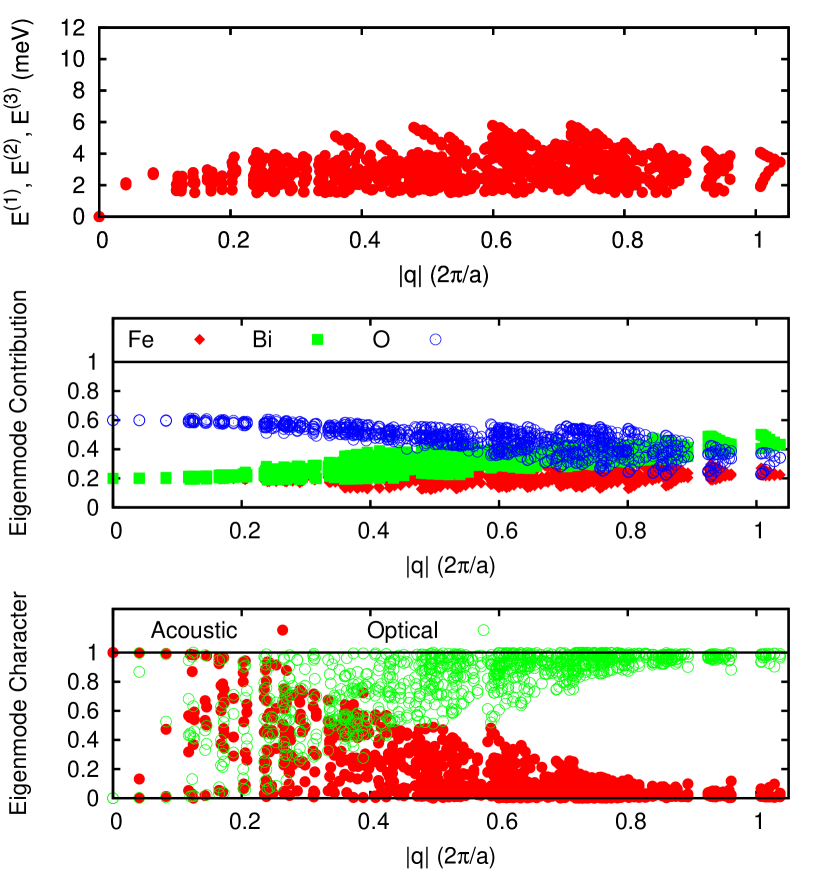
Figure 13: (Color online) Same as Fig. 7, but for the complex ${\cal C}$ phase considered in this work.

Novel nanoscale-twinned structures, denoted here as complex or ${\cal C}$ phases, have been recently suggested to stabilize in bulk BFO under conditions of high-$T$ or high-$p$, and upon appropriate chemical substitutions.prosandeev12 From a structural point of view, these ${\cal C}$ phases can be thought of a bridge appearing whenever we have ${\cal R}$ and ${\cal O}$ regions in the phase diagram of BFO. Thus, the energies of the nanoscale-twinned structures lie very close to that of the ground state. Interestingly, these ${\cal C}$ phases have been linked also to the structure of domain walls whose energy is essentially determined by antiferrodistortive modes involving the rotation of O₆ octahedra.dieguez13 These intriguing features motivated us to study the thermodynamic stability of this new type of phases with the QH approach. We note that, in the original paper by Prosandeev et al.,prosandeev12 several phases are proposed as members of the ${\cal C}$ family. For reasons of computational affordability, we restrict our analysis here to one particular structure (with $Pca2_{1}$ space group and $Z=8$) that has been introduced above and is depicted in Fig. 1(d).

In Fig. 12 we plot the QH free energy of our ${\cal C}$ phase expressed as a function of temperature, taking the result for the ${\cal R}$ structure as the zero of energy. As one may observe there, at low $T$ the $\Delta F_{\rm qh}$ difference is negative and quite small in absolute value. At $T=0$ K, for instance, this quantity amounts to $-$0.025 (5) eV/f.u., and roughly lies between the values corresponding to the ${\cal T}$ and ${\cal O}$ phases. As $T$ is raised, however, $\Delta F_{\rm qh}$ increases steadily with an approximate slope of $2\times 10^{-5}$ eV/K, and at $T\approx 1000$ K it becomes positive within our numerical uncertainties. This change of sign marks the occurrence of a potential ${\cal R}\to{\cal C}$ transformation. However, such a transition would be prevented by the onset of the ${\cal O}$ phase, which becomes the equilibrium state at a lower temperature. Note that, according to our results, the prevalence of the ${\cal O}$ phase occurs in spite of the fact that, at 0 K, this phase is energetically less favorable than the ${\cal C}$ state by 0.021 eV/f.u.

The free energy competition between the ${\cal O}$ and ${\cal C}$ phases is very strong, as can be deduced from the pDOS plots enclosed in Fig. 5. In particular, the ${\cal C}$ phase shares common pDOS features with both the ${\cal R}$ and ${\cal O}$ structures, which is hardly surprising given that its atomic arrangement can be viewed as a mixture between the ${\cal R}$ and ${\cal O}$ solutions. For instance, in the $\omega\to 0$ limit, the ${\cal C}$ and ${\cal O}$ distributions are practically identical, and the range of phonon frequencies over which they expand is very similar. Moreover, the number of low-lying optical phonon modes found in the ${\cal C}$ phase is, as we calculated for the ${\cal O}$ structure, very high (although we note that in the ${\cal C}$ case the contribution of the Fe anions to the eigenmodes is not negligible, see Fig. 13). Then, for intermediate frequencies the ${\cal C}$ pDOS presents a series of modulations which are more characteristic of the ${\cal R}$ phase. Also, the energy of the first ${\cal C}$ pDOS peak is closer to that of the ${\cal R}$ phase, and from an elastic point of view both ${\cal C}$ and ${\cal R}$ phases are very similar (that is, the bulk modulus of the two structures are coincident within our numerical uncertainties). A quantitative testimony of these pDOS similarities is given by the geometric frequencies $\bar{\omega}$ calculated in the ${\cal O}$, ${\cal C}$, and ${\cal R}$ phases, which are 27.16 meV, 28.00 meV, and 28.58 meV, respectively. Furthermore, ZPE corrections in the ${\cal C}$ phase amount to 0.254 eV/f.u., a value that roughly coincides with the arithmetic average obtained for the corresponding ${\cal O}$ and ${\cal R}$ results. In conclusion, we can state that BFO in the ${\cal C}$ phase is in average vibrationally softer than in the ${\cal R}$ phase, but more rigid than in the ${\cal O}$ phase.

It is worth noticing that, although we do not predict here a temperature-induced phase transition of the ${\cal R}\to{\cal C}$ type, this can not be discarded to occur in practice given that the calculated $\Delta F_{\rm qh}$ differences among the ${\cal R}$, ${\cal O}$ and ${\cal C}$ structures are very small. Note that small variations in the computed free energies – as for instance due to the use of a different exchange-correlation functional in our DFT calculations, related to our QH approximation, etc. – could very well change this delicate balance of relative stability (see discussion in Sec. III.7). Further, the ${\cal C}$ phase considered here is only one among the many nanoscale-twinned structures that have been predicted to exist,prosandeev12 and it is reasonable to speculate that some of them might indeed be predicted to be the equilibrium solutions by the DFT scheme employed here. At any rate, our results do suggest that these ${\cal C}$ structures are, at the very least, very close to becoming stable in the regions of the phase diagram in which ${\cal R}\to{\cal O}$ transitions occur. Moreover, they are obvious candidates to mediate (i.e., to appear in the path of) the ${\cal R}\to{\cal O}$ transformation. Hence, our results are clearly compatible with the possibility that ${\cal C}$ phases can be accessed experimentally, as robust meta-stable states, depending on kinetic factors.

III.5 The super-tetragonal ${\cal T}$ phase

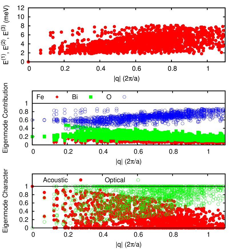
Figure 14: (Color online) Same as Fig. 7, but for the super-tetragonal ${\cal T}$ phase considered in this work.

Under zero $p-T$ conditions, the energy of the ${\cal T}$ structure depicted in Fig. 1(d) differs from that of the ${\cal R}$ phase by only few hundredths of eV per formula unit.dieguez11 This ${\cal T}$ phase possesses a giant $c/a$ ratio, a large electric polarization with a small in-plane component, and anti-ferromagnetic spin order of type C (C-AFM); hence, in principle, this phase would be potentially relevant for technological applications. Nevertheless, the ${\cal T}$ phase has never been observed in bulk samples of BFO (although it is stabilized in thin films under high compressive and tensile epitaxial constraintbea09 ; zeches09 ). Aiming at understanding the causes behind the frustrated stabilization of a bulk-like ${\cal T}$ phase in BFO, we studied it with the QH approach.

In Fig. 12 we plot the QH free energy of the ${\cal T}$ phase taken with respect to that of the ${\cal R}$ structure and expressed as a function of temperature. The ${\cal T}$ phase is assumed to present frozen C-AFM spin order, and a frozen G-AFM arrangement is considered for the ${\cal R}$ phase. As one may observe there, the free energy difference $\Delta F_{\rm qh}(T)$ is negative and very small at low temperatures (e.g., $\Delta F_{\rm qh}$(0 K) = $-$0.012 (5) eV/f.u.) but progressively increases in absolute value as $T$ is raised (e.g., $\Delta F_{\rm qh}$(1000 K) = $-$0.078 (5) eV/f.u.). This result implies that vibrational thermal excitations energetically destabilize the ${\cal T}$ phase as compared to the ${\cal R}$ and ${\cal O}$ structures, in agreement with observations.

This conclusion may not seem so obvious from inspection of the pDOS results enclosed in Fig. 5. As we can see there, at frequencies below 5 meV, the ${\cal T}$ phase presents a larger phonon density than the ${\cal R}$ phase, which would in principle suggest that the ${\cal T}$ structure is vibrationally softer. However, the lowest-lying pDOS peak in the ${\cal R}$ phase is much higher than in the ${\cal T}$ structure, and this feature turns out to be dominant. In particular, the calculated geometric frequency $\bar{\omega}$ amounts to 33.07 meV in the ${\cal T}$ phase and to 28.58 meV in the ground state. Interestingly, ZPE corrections (see Eq. 7) in both ${\cal R}$ and ${\cal T}$ phases are practically identical ($\sim$ 0.26 eV/f.u.).

The relatively high number of phonon modes that the ${\cal T}$ phase presents at very low frequencies is reminiscent of the results discussed above for the ${\cal O}$ structure. Indeed, as can be seen in Fig. 14, in the ${\cal T}$ phase we also find low-lying phonons of very low energy throughout the BZ. Additionally, the ${\cal T}$ phase also presents a relatively small bulk modulus and is elastically softer than the ${\cal R}$ structure: we obtained 73(2) GPa in this case, while we calculated 99(2) GPa for the ${\cal R}$ phase. These bulk modulus results are consistent with what one would generally expect from inspection of the pDOS plots enclosed in Fig. 5; in this sense, the ${\cal T}$ structure behaves normally, in contrast with the behavior of the ${\cal O}$ structure discussed above. Finally, let us note that, as shown in Fig. 14, the lowest-energy phonons of the ${\cal T}$ phase are largely dominated by the oxygen cations. This results is in contrast with our findings for the ${\cal R}$, ${\cal O}$, and ${\cal C}$ structures. Such a differentiated behavior is probably related to the fact that, unlike to all the other phases, the basic building block of the ${\cal T}$ structure are O₅ pyramids [see Fig. 1(c)]; having so many oxygen-dominated low-frequency modes suggests that such pyramids are more easily deformable than the rather rigid O₆ octahedra characteristic of the other phases.

III.6 Pressure-induced transitions at 0 K

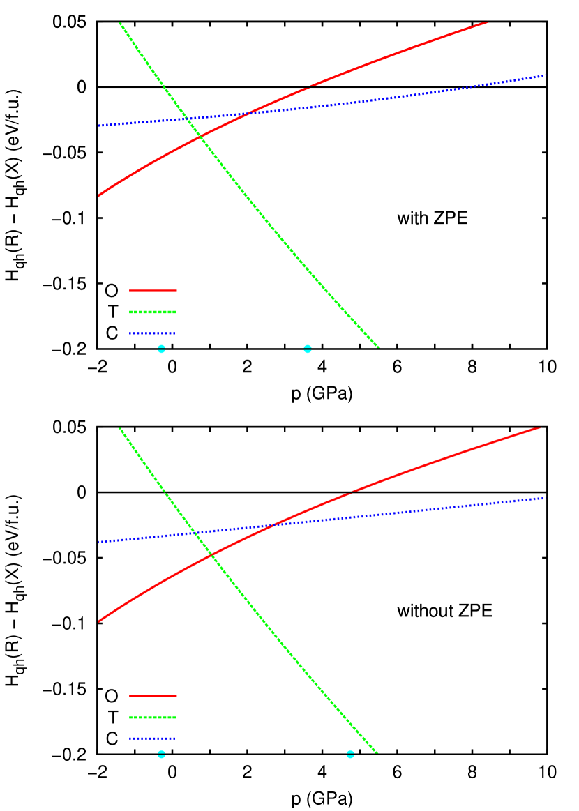
Figure 15: (Color online) Calculated enthalpy energy differences among the four crystal structures analyzed in this work, at $T=0$ K and expressed as a function of $p$. Results obtained when considering (resp. neglecting) ZPE corrections are shown in the top (resp. bottom) panel. Blue dots in the pressure axis mark the occurrence of first-order phase transitions (i.e., $\Delta H_{\rm qh}(p_{t})=0$).

$R3c-G$		$a=5.606$ Å	$b=5.606$ Å	$c=13.950$ Å
${\rm(P~{}=~{}3.6~{}GPa)}$		$\alpha=90~{}^{\circ}$	$\beta=90~{}^{\circ}$	$\gamma=120~{}^{\circ}$
${\rm Atom}$	${\rm Wyc.}$	$x$	$y$	$z$
${\rm Bi}$	$6a$	$0.0$	$0.0$	$0.4959$
${\rm Fe}$	$6a$	$0.0$	$0.0$	$0.2734$
${\rm O}$	$18b$	$0.4186$	$-0.0174$	$0.0402$
$Pnma-G$		$a=5.696$ Å	$b=7.838$ Å	$c=5.465$ Å
${\rm(P~{}=~{}3.6~{}GPa)}$		$\alpha=90~{}^{\circ}$	$\beta=90~{}^{\circ}$	$\gamma=90~{}^{\circ}$
${\rm Atom}$	${\rm Wyc.}$	$x$	$y$	$z$
${\rm Bi}$	$4c$	$0.0512$	$0.25$	$0.5098$
${\rm Fe}$	$4a$	$0.0$	$0.0$	$0.0$
${\rm O}$	$4c$	$-0.0285$	$0.25$	$0.0960$
${\rm O}$	$8d$	$0.1998$	$-0.0469$	$0.3044$

Table 2: Calculated structural data corresponding to the $p$-induced ${\cal R}\to{\cal O}$ transition that is predicted when quantum ZPE corrections are considered. Wyckoff positions were generated with the ISOTROPY package.isotropy

In this section we analyze the thermodynamic stability of the four studied crystal structures under hydrostatic pressure at $T=0$ K. We take into account ZPE corrections and consider also negative pressures.

In Fig. 15 we plot the enthalpy energy (i.e., $H=E+pV$) of the ${\cal O}$, ${\cal T}$, and ${\cal C}$ phases as a function of $p$, taking the result for the ${\cal R}$ structure as the pressure-dependent zero of enthalpy. A first-order transformation between phases $A$ and $B$ occurs at pressure $p_{t}$ when the enthalpy energy difference $\Delta H(p_{t})\equiv H_{A}-H_{B}$ becomes zero. In all the cases we present the results obtained both when neglecting ZPE corrections (i.e., for $E=E_{\rm eq}$ and $p=-\partial E_{\rm eq}/\partial V$) and when fully considering them (i.e., for $E=E_{\rm eq}+F_{\rm harm}(T\to 0)$ and $p=-\partial[E_{\rm eq}+F_{\rm harm}(T\to 0)]/\partial V$). Additional phonon and static energy calculations were performed whenever required in order to compute accurate enthalpies in the pressure interval $-$2 GPa $\leq p\leq$ 10 GPa.

As we increase the pressure, we find two phase transitions of the ${\cal T}\to{\cal R}$ and ${\cal R}\to{\cal O}$ types. The ${\cal T}\to{\cal R}$ transition occurs at $-$0.3(1) GPa and the associated volume change is $\Delta V=6.76$ Å³/f.u.; at this transition pressure, the ${\cal T}$ phase presents a volume of 71.94 Å³/f.u. and a very large $c/a$ ratio of about 2. The ${\cal R}\to{\cal O}$ transition occurs at 3.6(1) GPa, and the volume changes from 63.04 Å³/f.u. to 61.13 Å³/f.u.; the corresponding structural data is given in Table II. Interestingly, the pressure-dependence of the enthalpies shown in Fig. 15 resemble the results reported in Fig. 12 for $F_{\rm qh}$ as a function of temperature. In particular, under compression the ${\cal T}$ phase becomes higher in enthalpy than the rest, and the enthalpy of the ${\cal O}$ phase turns out to be the smallest. Also, the ${\cal C}$ phase gets energetically favored over the ${\cal R}$ structure upon increasing pressure, although it never becomes the most stable structure.

The bottom panel in Fig. 15 shows the enthalpy results obtained when ZPE corrections are neglected. Interestingly, while the main trends are conserved, the pressure of the ${\cal R}\to{\cal O}$ transformation turns out to be shifted up to 4.8(1) GPa. This result shows that atomic quantum delocalization effects in perovskite oxides may be important for accurate prediction of $p$-induced phase transitions.

Our results for the ${\cal R}\to{\cal O}$ transformation are consistent with those of previous theoretical studies,ravindran06 ; dieguez11 the quantitative differences being related to the varying DFT flavors employed, consideration of typically-neglected ZPE corrections, and other technicalities. As regards the connection with experiment, it is worth noting that we predict the ${\cal R}\to{\cal O}$ transition to occur at a pressure (3.6 GPa) that is rather close to the one at which the ${\cal R}$ phase has been observed to transform into a complex structure by Guennou et al.guennou11 (i.e., $\sim$ 4 GPa at room temperature). It is therefore tempting to identify the experimentally detected complex structure with the family of ${\cal C}$ phases of which we have investigated a representative case; indeed, verifying a possible ${\cal R}\to{\cal C}\to{\cal O}$ transition sequence was one of our motivations to investigate the effects of pressure. However, our calculations render a direct ${\cal R}\to{\cal O}$ transition, which suggests that the experimentally observed complex structures might actually be very long-lived meta-stable states, as opposed to actual equilibrium phases. On the other hand, as explained in Section III.4, getting accurate predictions near transition points at which $F_{\rm qh}({\cal R})\approx F_{\rm qh}({\cal C})\approx F_{\rm qh}({\cal O})$ is clearly a challenging task, and many factors can come into play and affect the results. Hence, we cannot fully discard the possibility that, under pressure, the ${\cal R}$ structure transforms into a complex equilibrium phase.

III.7 The role of the exchange-correlation energy functional

In previous sections we have highlighted that the differences in the Helmholtz free energies and enthalpies of the ${\cal R}$, ${\cal O}$, and ${\cal C}$ phases are calculated to be exceedingly small. In such conditions, our predictions for the equilibrium phase may depend, among other factors, on the employed exchange-correlation DFT energy functional. In this sense, Diéguez et al. already founddieguez11 that, in BFO, energy differences between stable structures depend strongly on the DFT energy functional used, with variations in $E_{\rm eq}$ that may be as large as 0.1 eV per formula unit.

To estimate the magnitude of this type of uncertainties in our $\Delta F_{\rm qh}$ results computed with a PBE+$U$ functional, we repeated our QH investigation of temperature-driven transitions – at constant volume and frozen-spin conditions – using a LDA+$U$ scheme. Our LDA+$U$ results show, in accordance with the presented PBE+$U$ study, that the orthorhombic ${\cal O}$ phase gets thermodynamically stabilized over the rest of structures at high temperatures, and that the ${\cal T}$ phase goes steadily higher in free energy. Further, the LDA+$U$ results indicate that the ${\cal R}\to{\cal O}$ transition occurs at approximately 500 K, which is much lower than the experimental result. Interestingly, most of the the discrepancy between this LDA+$U$ result and our PBE+$U$ prediction (900 K) can be traced back to the different equilibrium energies in the 0 K limit, with the phonon contributions to the free energy playing a secondary role. Indeed, from the PBE+$U$ calculations we get $E_{\rm eq}({\cal O})-E_{\rm eq}({\cal R})$ =$-0.061$ eV/f.u., while the LDA+$U$ result is $-0.016$ eV/f.u. Obviously, the LDA+$U$ functional brings the ${\cal R}$ and ${\cal O}$ phases much closer in energy, which leads to the stabilization of the ${\cal O}$ structure at a much lower temperature. Additionally, the $F_{\rm qh}$ of the ${\cal C}$ phase remains always about 50 meV/f.u. higher than that of the ${\cal R}$ phase, the difference being weakly dependent on temperature.

Hence, our calculations confirm that quantitative predictions of transition temperatures are strongly dependent on the employed DFT functional. We can also conclude that the LDA functional does not capture properly the relative stability of the ${\cal R}$ and ${\cal O}$ phases of BFO, and that the PBE functional is a much better choice. In this sense, our work ratifies the conclusions presented in Ref. dieguez11, .

IV Conclusions

We have performed a first-principles study of the $p-T$ phase diagram of bulk multiferroic BFO relying on quasi-harmonic free energy calculations. We have analyzed the thermodynamic stability of four different crystal structures that have been observed, or predicted to exist, at normal and high $p$ or $T$ conditions and/or in thin films under epitaxial constraints. In order to incorporate the effects of spin-phonon coupling on the quasi-harmonic calculation of the Helmholtz free energies, we have developed an approximate and technically simple scheme that allows us to model states with varying degrees of spin disorder.

Consistent with observations, we find that the rhombohedral $R3c$ ferroelectric phase (${\cal R}$ phase) is the ground state of the material at ambient conditions of pressure. Then, an orthorhombic $Pnma$ structure (${\cal O}$ phase), which is the vibrationally-softest of all the considered structures, is found to stabilize upon increasing $T$ or $p$. More precisely, two first-order phase transitions of the $R\to O$ type are predicted to occur at the thermodynamic states [0 GPa, 1300(100) K] and [3.6(1) GPa, 0 K].

Additionally, a representative of the so-called nano-twinned structures recently predicted to occur in BFOprosandeev12 has been analyzed in this work. This phase is found to display elastic and vibrational features that are reminiscent of the results obtained for both the ${\cal R}$ and ${\cal O}$ structures, and to become energetically more stable than the ${\cal R}$ phase upon raising $p$ and $T$. The entropy and enthalpy of the ${\cal O}$ phase, however, turn out to be more favorable than those of the studied ${\cal C}$ structure over practically all the investigated $p-T$ intervals, and as a result we do not observe any direct ${\cal R}\to{\cal C}$ or ${\cal C}\to{\cal O}$ transformation. Nevertheless, our results cannot be conclusive in this point due to the limitations of the study (only one specific nano-twinned structure is investigated) and DFT-related accuracy problems that appear when tackling very small free-energy differences (i.e., of order $1-10$ meV/f.u.). In fact, our results seem to support the possibility that some nano-twinned structures may become stable at the boundaries between ${\cal R}$ and ${\cal O}$ phases in the $p-T$ phase diagram of BFO, or at least exist as long-lived meta-stable phases that are likely to be accessed depending on the kinetics of the ${\cal R}\to{\cal O}$ transformation.

Finally, we find that a representative of the so-called super-tetragonal phases of BFO gets energetically destabilized over the rest of crystal structures by effect of increasing temperature, due to the fact that its spectrum of phonon frequencies is globally the stiffest one. This explains why super-tetragonal structures have never been observed in bulk BFO, in spite of the fact that their DFT-predicted energies are very close to those of the ${\cal R}$ and ${\cal O}$ phases. Interestingly, the investigated super-tetragonal structure is also destabilized upon hydrostatic compression.

As far as we know, our work is the first application of the quasi-harmonic free energy method to the study of the phase diagram of a multiferroic perovskite system. The main advantages of this approach are that is computationally affordable, can be straightforwardly applied to the study of crystals, and naturally incorporates zero-point energy corrections. Among its shortcomings, we note that it can be exclusively applied to the analysis of vibrationally stable crystal structures; further, it only incorporates anharmonic effects via the volume-dependence of the phonon frequencies and corresponding treatment of the thermal expansion, which may be a questionable approximation at high temperatures. Nevertheless, we may think of several physically interesting (and computationally very challenging) situations involving BFO-related multiferroics in which the present approach can prove to be especially useful. A particularly interesting possibility pertains to the study of solid solutions, i.e., bulk mixtures of two or more compounds, at finite temperatures. By assuming simple (or not so simple) relations among the free energy of the composite system, the relative proportion between the species, and the vibrational features of the integrating bulk compounds, one may be able to estimate the phase boundaries in the complicated $x$-$p$-$T$ phase diagrams at reasonably modest computational effort. In this regard, the BiFeO₃-BiCoO₃ and BiFeO₃-LaFeO₃ solid solutions emerge as particularly attractive cases, since the application electric fields in suitably prepared materials can potentially trigger the switching between different ferroelectric-ferroelectric and ferroelectric-paraelectric phases.dieguez11b ; otto12

Beyond possible applications, studying the BiFeO₃-BiCoO₃ solid solution is by itself very interesting. On the one hand, this is a case involving transitions between phases that are very dissimilar structurally (super-tetragonal and quasi-rhombohedral), and which have different magnetic orders (C-AFM and G-AFM). Hence, in this case we can expect spin-phonon effects to have a larger impact in the free energy, which would allow us to better test the spin-phonon quasi-harmonic approach that we have introduced in the present work. Additionally, the treatment of the C-AFM order requires a more complicated model of exchange interactions, involving at least two (preferably threeescorihuela12 ) coupling constants. Hence, treating C-AFM phases requires a extension of the scheme here presented, so that it can easily tackle more general situations. Work in this direction is already in progress within our group.

- (1) M. Fiebig, J. Phys. D 38, R123 (2005).
- (2) M. Fiebig, Phase Transitions 79, 947 (2006).
- (3) R. Ramesh and N. A. Spaldin, Nature Mater. 6, 21 (2007).
- (4) W. Eerenstein, N. D. Mathur, and J. F. Scott, Nature (London) 442, 759 (2006).
- (5) N. Balke et al., Nature Phys. 8, 81 (2012).
- (6) P. Rovillain, R. de Sousa, Y. Gallais, A. Sacuto, M. Measson, D. Colson, A. Forget, M. Bibes, A. Barthelemy, and M. Cazayous, Nature Mater. 9, 975 (2010).
- (7) M. Gajek, M. Bibes, S. Fusil, K. Bouzehouane, J. Fontcuberta, A. Barthlmy, and A. Fert, Nature Mater. 6, 296 (2007).
- (8) S. V. Kiselev, R. P. Ozerov, and G. S. Zhdanov, Sov. Phys. Dokl. 7, 742 (1963).
- (9) G. A. Smolenskii, V. A. Isupov, A. I. Agranovskaya, and N. N. Krainik, Sov. Phys. Solid State 2, 2651 (1961).
- (10) G. Catalan and J. F. Scott, Adv. Mater. 21, 2463 (2009).
- (11) S. Lee, W. Ll. Ratcliff, S.-W. Cheong, and V. Kiryukhin, Appl. Phys. Lett. 92, 192906 (2008).
- (12) D. Lebeugle, D. Colson, A. Forget, M. Viret, A. M. Bataille, and A. Gukasov, Phys. Rev. Lett. 100, 227602 (2008).
- (13) T. Zhao et al., Nat. Mats. 5, 823 (2006).
- (14) A. M. Glazer, Acta Crystallogr. Sect. A 31, 756 (1975).
- (15) R. Haumont, J. Kreisel, and P. Bouvier, Phys. Rev. B 73, 132101 (2006).
- (16) R. Palai, R. S. Katiyar, H. Schmid, P. Tissot, S. J. Clark, J. Robertson, S. A. T. Refern, G. Catalan, and J. F. Scott, Phys. Rev. B 77, 014110 (2008).
- (17) I. A. Kornev, S. Lisenkov, R. Haumont, B. Dkhil, and L. Bellaiche, Phys. Rev. Lett. 99, 227602 (2007).
- (18) R. Haumont, I. A. Kornev, S. Lisenkov, L. Bellaiche, J. Kreisel, and B. Dkhil, Phys. Rev. B 78, 134108 (2008).
- (19) D. C. Arnold, K. S. Knight, F. D. Morrison, and P. Lightfoot, Phys. Rev. Lett. 102, 027602 (2009).
- (20) In Arnold’s original work the paraelectric -phase is designated as . Actually orthorhombic ABO3 perovskites have space group (in accordance with crystallographic conventions), and both and space groups are equivalent and related via a simple transformation. Within the physics community, however, refering to the space group appears to be more popular.
- (21) P. Ravindran, R. Vidya, A. Kjekshus, H. Fjellvag, and O. Eriksson, Phys. Rev. B 74, 224412 (2006).
- (22) R. Haumont, P. Bouvier, A. Pashkin, K. Rabia, S. Frank, B. Dkhil, W. A. Crichton, C. A. Kuntscher, and J. Kreisel, Phys. Rev. B 79, 184110 (2009).
- (23) M. Guennou, P. Bouvier, G. S. Chen, B. Dkhil, R. Haumont, G. Garbarino, and J. Kreisel, Phys. Rev. B 84, 174107 (2011).
- (24) S. Prosandeev, D. Wang, W. Ren, J. iguez, and L. Bellaiche, Adv. Funct. Mater. 23, 234 (2013).
- (25) O. Diguez, O. E. Gonzlez-Vzquez, J. C. Wojdeł and J. iguez, Phys. Rev. B 83, 094105 (2011).
- (26) L. Bellaiche and J. Íñiguez, Phys. Rev. B 88, 014104 (2013).
- (27) O. Diguez, P. Aguado-Puente, J. Junquera, and J. iguez, Phys. Rev. B 87, 024102 (2013).
- (28) H. Ba, B. Dup, S. Fusil, R. Mattana, E. Jacquet, B. Warot-Fonrose, F. Wilhelm, A. Rogalev, S. Petit, V. Cros, A. Anane, F. Petroff, K. Bouzehouane, G. Geneste, B. Dkhil, S. Lisenkov, I. Ponomareva, L. Bellaiche, M. Bibes, and A. Barthlmy, Phys. Rev. Lett. 102, 217603 (2009).
- (29) R.J. Zeches et al., Science 326, 977 (2009).
- (30) B. Dup, I.C. Infante, G. Geneste, P.-E. Janolin, M. Bibes, A. Barthlmy, S. Lisenkov, L. Bellaiche, S. Ravy, and B. Dkhil, Phys. Rev. B 81, 144128 (2010).
- (31) W. Zhong, D. Vanderbilt, and K. M. Rabe, Phys. Rev. Lett. 73, 1861 (1994).
- (32) W. Zhong, D. Vanderbilt, and K. M. Rabe, Phys. Rev. B 52, 6301 (1995).
- (33) U. V. Waghmare and K. M. Rabe, Phys. Rev. B 55, 6161 (1997).
- (34) Y.-H. Shin, V.R. Cooper, I. Grinberg, and A.M. Rappe, Phys. Rev. B 71, 054104 (2005)
- (35) M. Sepliarsky, A. Asthagiri, S.R. Phillpot, M.G. Stachiotti, and R.L. Migoni, Current Opinion in Sol. St. and Mats. Sci. 9, 107 (2005).
- (36) J.C. Wojdeł, P. Hermet, M.P. Ljungberg, P. Ghosez, and J. Íñiguez, J. Phys.: Condens. Matt. 25, 305401 (2013).
- (37) D. Rahmedov, D. Wang, J. iguez, and L. Bellaiche, Phys. Rev. Lett. 109, 037207 (2012).
- (38) C. Cazorla, D. Alfè, and M. J. Gillan, Phys. Rev. Lett. 101, 049601 (2008).
- (39) S. Shevlin, C. Cazorla, and Z. X. Guo, J. Phys. Chem. C 116, 13488 (2012).
- (40) C. Cazorla, D. Alfè, and M. J. Gillan, Phys. Rev. B 85, 064113 (2012).
- (41) C. Cazorla and D. Errandonea, Phys. Rev. B 81, 104108 (2010).
- (42) S. Taioli, C. Cazorla, M. J. Gillan, and D. D. Alfè, Phys. Rev. B 75, 214103 (2007).
- (43) C. Cazorla, M. J. Gillan, S. Taioli, and D. D. Alfè, J. Chem. Phys. 126, 194502 (2007).
- (44) C. Cazorla, D. Errandonea and E. Sola, Phys. Rev. B 80, 064105 (2009).
- (45) C.J. Fennie and K.M. Rabe, Phys. Rev. Lett. 97, 267602 (2006).
- (46) J. H. Lee and K. M. Rabe, Phys. Rev. Lett. 104, 207204 (2010).
- (47) J. Hemberger, T. Rudold, H.-A. Krug von Nidda, F. Mayr, A. Pimenov, V. Tsurkan, and A. Loidl, Phys. Rev. Lett. 97, 087204 (2006).
- (48) T. Rudolf, C. Kant, F. Mayr, and A. Loidl, Phys. Rev. B 77, 024421 (2008).
- (49) J. Hong, A. Stroppa, J. iguez, S. Picozzi, and D. Vanderbilt, Phys. Rev. B 85, 054417 (2012).
- (50) F. Körmann, A. Dick, B. Grabowski, B. Hallstedt, T. Hickel, and J. Neugebauer, Phys. Rev. B 78, 033102 (2008).
- (51) S.-L. Shang, Y. Wang, and Z.-K. Liu, Phys. Rev. B 82, 014425 (2010).
- (52) F. Körmann, A. Dick, B. Grabowski, T. Hickel, and J. Neugebauer, Phys. Rev. B 85, 125104 (2012).
- (53) J. P. Perdw, K. Burke, and M. Ernzerhof, Phys. Rev. Lett. 77, 3865 (1996).
- (54) G. Kresse and J. Fürthmuller, Phys. Rev. B 54, 11169 (1996); G. Kresse and D. Joubert, Phys. Rev. B 59, 1758 (1999).
- (55) P. E. Blöchl, Phys. Rev. B 50, 17953 (1994).
- (56) S. Baroni, P. Giannozzi, and A. Testa, Phys. Rev. Lett. 58, 1861 (1987).
- (57) S. Baroni, S. de Gironcoli, A. Dal Corso, and P. Giannozzi, Rev. Mod. Phys. 73, 515 (2001).
- (58) X. Gonze and J.-P. Vigneron, Phys. Rev. B 39, 13120 (1989).
- (59) X. Gonze and C. Lee, Phys. Rev. B 55, 10355 (1997).
- (60) G. Kresse, J. Furthmüller, and J. Hafner, Europhys. Lett. 32, 729 (1995).
- (61) D. Alfè, G. D. Price, and M. J. Gillan, Phys. Rev B 64, 045123 (2001).
- (62) D. Alfè, Comp. Phys. Commun. 180, 2622 (2009).
- (63) H. J. Monkhorst and J. D. Pack, Phys. Rev. B 13, 5188 (1976).
- (64) D. Alfè, program available at http://chianti.geol.ucl.ac.uk/ dario (1998).
- (65) W. Cochran and R. A. Cowley, J. Phys. Chem. Solids 23, 447 (1962).
- (66) Y. Wang, J. J. Wang, W. Y. Wang, Z. G. Mei, S. L. Shang, L. Q. Chen, and Z. K. Liu, J.Phys.:Condens. Matter 22, 202201 (2010).
- (67) J. Hlinka, J. Pokorny, S. Karimi, and I. M. Reaney, Phys. Rev. B 83, 020101(R) (2011).
- (68) E. Borissenko et al., J. Phys.:Condens. Matter 25, 102201 (2013).
- (69) P. Hermet, M. Goffinet, J. Kreisel, and Ph. Ghosez, Phys. Rev. B 75, 220102(R) (2007).
- (70) Y. Wang, J. E. Saal, P. Wu, J. Wang, S. Shang, Z.-K. Liu, and L.-Q. Chen, Acta Materialia 59, 4229 (2011).
- (71) Given the lattice-periodic part of a particular phonon eigenmode , we calculate its polarity as , where runs over atoms in the unit cell, and are Cartesian directions, and is the Born effective charge tensor for atom .
- (72) C. Escorihuela-Sayalero, O. Diguez, and J. iguez, Phys. Rev. Lett. 109, 247202 (2012).
- (73) F. Birch, J. Geophys. Res. 83, 1257 (1978).
- (74) C. Cazorla and D. Errandonea, J. Phys. Chem. C 117, 11292 (2013).
- (75) H. T. Stokes, D. M. Hatch, and B. J. Campbell, (2007). ISOTROPY, stokes.byu.edu/isotropy.html.
- (76) O. Diguez and J. iguez, Phys. Rev. Lett. 107, 057601 (2011).
- (77) O. E. Gonzlez-Vzquez, J. C. Wojdeł, O. Diguez, and J. iguez, Phys. Rev. B 85, 064119 (2012).
- (78) K. Momma and F. Izumi, J. Appl. Crystallogr. 41 , 653 (2008).