Sample and Hold Errors in the Implementation of Chaotic Maps

Abstract

Though considerable effort has recently been devoted to hardware realization of chaotic maps, the analysis generally neglects the influence of implementation inaccuracies. Here we investigate the consequences of S/H errors on Bernoulli shift, tent map and tailed tent map systems: an error model is proposed and implementations are characterized under its assumptions.

I Introduction

Silicon implementations of chaotic maps are analog discrete-time systems exploiting sample and hold (S/H) stages to introduce the necessary delay in the feedback loop (figure 1).

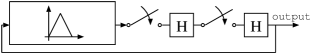
Figure 1: Basic piecewise affine unidimensional chaotic loop. Two S/H stages are needed to hold the map input stable while the map circuit produces its output.

Several efforts have recently been devoted to this area, identifying current mode techniques as the most reliable and effective design approach [1, 2, 3]. The many applications fields, including secure communication [4], noise generation, stochastic neural models [5], EMI reduction, etc., have directed the attention mainly in obtaining interesting chaotic behavious at the minimal hardware cost. On the contrary, the influence of implementation inaccuracies has often been neglected, particularly due to the difficulties inherent in relating the statistical properties of chaotic systems to their implementation errors. Herein, a sample and hold error model is developed and its correlation with operating frequencies is suggested. Three maps characterized by a uniform invariant probability density function (PDF) are then considered — the Bernoulli shift, the tent map, and the tailed tent map— and their implementation is characterized using this error model. Particularly, influence of errors on the statistical properties of the resulting signals is investigated, together with robustness issues. As a conclusion, the a superior performance of the tailed tent map is verified, and some design guidelines are drawn. Focusing on S/H errors is justified by the considerable overhead carried by most clock feedthrough reduction techniques and by their general unscalability in terms of the benefits one needs to achieve.

II Systems under investigation

Without any loss of generality, we shall consider normalized maps, i.e. maps whose invariant set (IS) is $[0,1]$. For a generic map $M$ having IS $[x_{h},x_{l}]$ a normalization function is defined as:

$$N(x)=(x-x_{l})/(x_{h}-x_{l})$$ (1)

so that $M_{n}(x)=N(M(N^{-1}(x)))$ is the corresponding normalized map.

The systems under investigation are those based on the Bernoulli shift (BS), the tent map (TM) and the tailed tent map (TTM) [3] (figure 2). All the systems are characterized by a uniform PDF. The normalized maps are given by:

$$M_{n}(x) =2x-\chi_{\{x>1/2\}}(x)$$ (2)

$$M_{n}(x) =1-2|x-1/2|$$ (3)

$$M_{n}(x) =1-2|x-\overline{t}/2|+\max(x-\overline{t},0)$$ (4)

respectively, where $\chi$ is a set characteristic function, $\overline{t}=1-t$ and $t$ is a fraction which controls the tail size in the TTM.

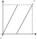
[-0.15cm] (BS)

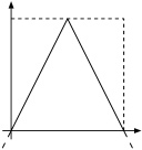
[-0.15cm] (TM)

[-0.15cm] (TTM)

Figure 2: Maps in the systems under investigation: Bernoulli shift, tent map and tailed tent map.

In order to evaluate the robustness of implemented chaotic maps, one must know how the map is defined out of its ideal IS [3]. For this purpose, we shall assume that maps extend out of their definition set by linear extrapolation of their edge branches (dashed lines in fig. 2).

Focusing on a limited number of maps allows the use of extensive to complement the achievable analyrical results.

III Modelling of sample and hold errors

Since two sample and hold stages are necessary to implement the feedback loop delay, we shall model both at once, up to the first derivative, as in:

$$\operatorname{sh}_{n}(x)=(1+\Delta\mu)x+\sigma_{n}-\frac{1}{2}\Delta\mu$$ (5)

where $\Delta\mu$ is a slope error and $\sigma_{n}$ is a normalized offset. Note that, once again, generality is preserved by means of normalization, so that the S/H model for a generic system would be

$$\operatorname{sh}(x)=N^{-1}\left((1+\Delta\mu)N(x)+\sigma_{n}-\frac{1}{2}\Delta\mu\right)$$ (6)

where $N$ is the normalization function (1). Since the ideal S/H behaviour is $\operatorname{sh}(x)=x$, $\Delta\mu$ and $\sigma_{n}$ are numeric indexes for the S/H error. Modelling up to the first derivative represents a compromise between accuracy and the need to keep error quantification simple and physically meaningful: $\Delta\mu$ and $\sigma_{n}$ correspond to the common concepts of signal dependent and signal independent S/H errors and appear useful for the present analysis. However higher order modelling would be necessary to accurately esteem errors on the statistics of implemented systems, as it will appear further on.

Note that a viable way to consider S/H errors is thinking of the ideal iteration of a perturbed map, which is a combination of the ideal map and the S/H characteristic. Finally, notice that in many chaotic map implementations the S/H stages represent the speed bottleneck due to a accuracy/sample-latency tradeoff: for any given S/H circuit $\Delta\mu$ and $\sigma_{n}$ can be reduced only by increasing the memory capacitance or by slowing the sample-to-hold commutation. Both actions limit the cycle frequency.

IV Characterization of implemented systems

Characterization of the implemented chaotic maps will be given by considering S/Hs as the sole error source and by looking at the following features:

Lack of robustness:

shown by total loss of the system characteristic behaviour (loss of chaoticity, acquisition of an IS which is not an interval).

Alteration of the invariant set:

S/H errors usually alter the set in which a chaotic system produces its samples. If $[x_{l},x_{h}]$ is the ideal IS and $[\tilde{x}_{l},\tilde{x}_{h}]$ is the IS due to S/H errors, the normalized IS error:

$$\epsilon_{b}=|N(\tilde{x}_{h})-1|+|N(\tilde{x}_{l})|$$ (7)

In some applications, $\epsilon_{b}$ may not be critical. Furthermore, it may be possible to track $\tilde{x}_{h}$ and $\tilde{x}_{l}$ dynamically $\epsilon_{b}$ by linear rescaling.

Alteration of the probability density function (PDF):

expressed using an $L_{1}$ norm. If $\psi$ be the ideal PDF and $\tilde{\psi}$ the real one, then the normalized PDFs are:

$$\psi_{n}(x) =(x_{h}-x_{l})\,\psi(N^{-1}(x))$$ (8)

$$\tilde{\psi}_{n}(x) =(\tilde{x}_{h}-\tilde{x}_{l})\,\tilde{\psi}(x\cdot(\tilde{x}_{h}-\tilde{x}_{l})+\tilde{x}_{l})$$ (9)

and the normalized PDF error is:

$$\epsilon_{\psi}=\int_{0}^{1}|\psi_{n}(x)-\tilde{\psi}_{n}(x)|\,dx$$ (10)

Notice that this valuation of the PDF error implies linear compensation of $\epsilon_{b}$.

Alteration of the cumulative probability density function (CDF):

evaluated using an $L_{1}$ norm. If $\Psi$ is the ideal cumulative probability density function (CDF) and $\tilde{\Psi}$ the real CDF, then the normalized CDFs are

$$\Psi_{n} =\Psi(N^{-1}(x))$$ (11)

$$\tilde{\Psi}_{n} =\tilde{\Psi}(x\cdot(\tilde{x}_{h}-\tilde{x}_{l})+\tilde{x}_{l})$$ (12)

and the normalized CDF error is:

$$\epsilon_{\Psi}=\int_{0}^{1}|\Psi_{n}(x)-\tilde{\Psi}_{n}(x)|\,dx$$ (13)

V Results and analysis

Characterization of map implementations achieved by simulation is shown in figures 3, 4 and 5 (error for a BS, a TM, and a TTM ($t=10\%$) based system): three surfaces and contours are plotted for each map, illustrating $\epsilon_{b}$, $\epsilon_{\psi}$ and $\epsilon_{\Psi}$ as a function of $\Delta\mu$ and $\sigma_{n}$. White areas in the contour plots represent loss of the system characteristic behaviour.

 
 
 

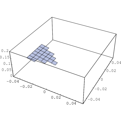
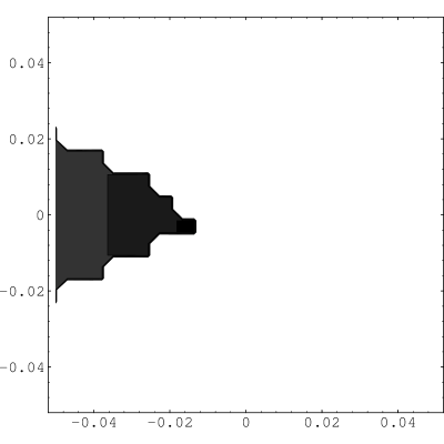
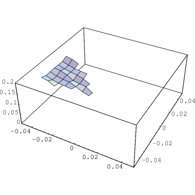
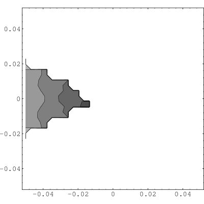
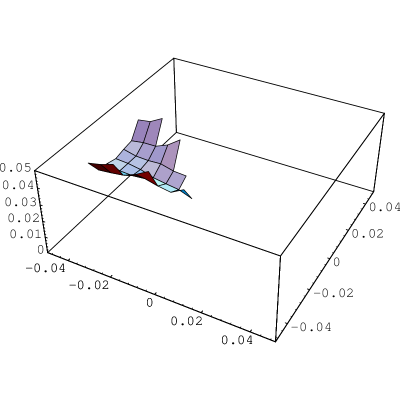
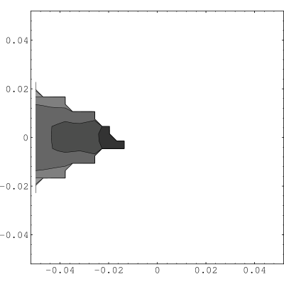
Figure 3: Behaviour of Bernoulli shift based systems in presence of S/H errors ($x$-axis: slope error $\Delta\mu$, $y$-axis: offset error $\sigma_{n}$). Top: IS bounds error; middle: PDF error; bottom CDF error. In contour plots darker regions represent lower errors, white regions are those where the system diverges.

 
 
 

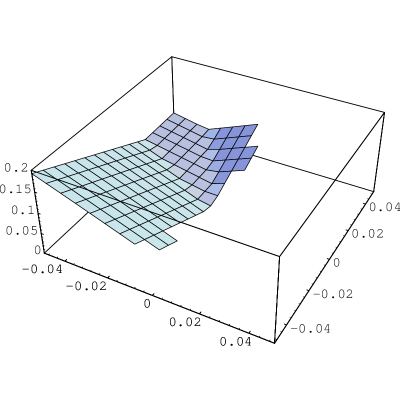
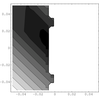
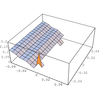
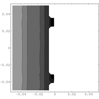
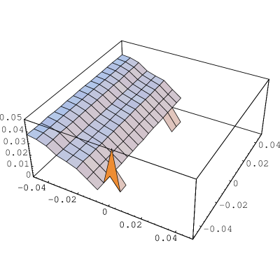
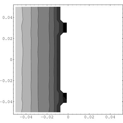
Figure 4: Behaviour of tent map based systems in presence of S/H errors. See also caption of figure 3

 
 
 

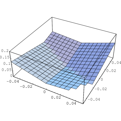
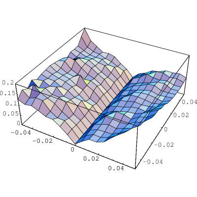
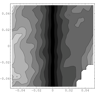
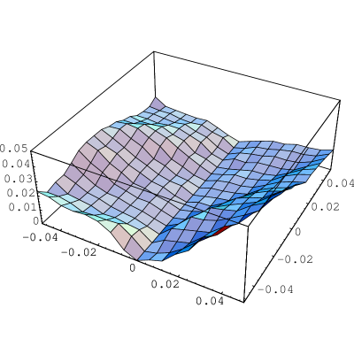
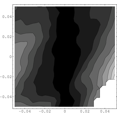
Figure 5: Behaviour of tailed tent map based systems in presence of S/H errors. See also caption of figure 3

For what concerns robustness and alterations in the invariant set, analytical results have been obtained in perfect accordance with simulations, while evaluation of errors on truly statistical properties (PDF, CDF) relies on numerical computations.

Robustness.

Non-allowable values of $\Delta\mu$ and $\sigma_{n}$ for which systems based on the BS, TM and TTM diverge can be determined analytically. Namely:

$$\begin{cases}\operatorname{sh}_{n}(0)>x_{0}&\text{for}\ x_{0}=\operatorname{sh}_{n}(2x_{0})\\ \operatorname{sh}_{n}(1)<x_{1}&\text{for}\ x_{1}=\operatorname{sh}_{n}(2x_{1}-1)\end{cases}$$ (14)

is the allowable region for the Bernoulli shift,

$$\operatorname{sh}_{n}(M_{n}(\operatorname{sh}_{n}(1)))>x_{0}\quad\text{for}\ x_{0}=\operatorname{sh}_{n}(2x_{0})\$$ (15)

for the tent map, and

$$\operatorname{sh}_{n}(M_{n}(\operatorname{sh}_{n}(1)))>x_{0}\quad\text{for}\ x_{0}=\operatorname{sh}_{n}(2x_{0}+t)\$$ (16)

for the tailed tent map. By substituting the proposed S/H model one gets:

$$\Delta\mu<2\sigma_{n}\quad\wedge\quad\Delta\mu<-2\sigma_{n}$$ (17)

$$\Delta\mu<0$$ (18)

$$\sigma_{n}>\frac{2\Delta\mu^{2}-3\Delta\mu-2t}{2(1-2\Delta\mu)}$$ (19)

respectively, which all find confirmation in the graphs.

In spite of the approximations in the S/H modelling, a clear tendency emerges: perturbations increasing the steepness of the BS and the TM ($\Delta\mu>0$) lead to systems diverging to infinity. For these maps, even ideal implementations can diverge if noise gets superimposed to the status variable (in fact $\Delta\mu=0$ does not belong to the allowable region). On the contrary, the TTM is tolerant to perturbation, showing a tolerance level which is controllable via parameter $t$ [3].

TM and BS systems can be made tolerant to perturbation by altering the maps outside their ideal IS. For instance, a hooked TM can be defined as $M(x)=1-2|x-1/2|+(2+a)\,\max(-x,0)$, with $a>2$. However, this is expensive, requiring an additional comparator to provide the hook breakpoint. Alternatively, robustness can be guaranteed by designing the systems so that the map steepness is made slightly lower than its stated value, but in this case robustness is paid in terms of PDF and CDF accuracy. Note that a way to lower the map steepness is to adopt a S/H topology characterized by $\Delta\mu>0$. Since this is not difficult to be done (see next section), in some sense S/H errors can be exploited to enhance the implementation robustness of certain systems.

Alteration of the invariant set.

For the BS one gets:

$$\tilde{x}_{h}=\operatorname{sh}(x_{h}),\quad\tilde{x}_{l}=\operatorname{sh}(x_{l})$$ (20)

while for both the TM and the TTM

$$\tilde{x}_{h}=\operatorname{sh}(x_{h}),\quad\tilde{x}_{l}=\operatorname{sh}(M(\tilde{x}_{h}))$$ (21)

Equations (20) and (21) (which are valid only for small errors) lead to

$$\epsilon_{b}=\left|\frac{1}{2}\Delta\mu+\sigma_{n}\right|+\left|-\frac{1}{2}\Delta\mu+\sigma_{n}\right|$$ (22)

$$\epsilon_{b}\approx\left|\frac{1}{2}\Delta\mu+\sigma_{n}\right|+\left|-\frac{3}{2}\Delta\mu-\sigma_{n}\right|$$ (23)

$$\epsilon_{b}\approx\left|\frac{1}{2}\Delta\mu+\sigma_{n}\right|+\left|-\Delta\mu\right|$$ (24)

for the BS, TM and TTM respectively (2nd order terms are neglected). Both the equations and the graphs, show that the TM is outperformed both by the BS and the TTM, the latter being generally the best.

Alteration of the PDF and the CDF.

As mentioned above, the analytical approach is not practicable to evaluate $\epsilon_{\psi}$ and $\epsilon_{\Psi}$. Nonetheless, simulation shows clearly that the three systems have similar performance in terms of PDF, while in terms of CDF the TTM performs better. Intuitively, a justification comes from considering that perturbed TTM systems tend to produce highly oscillatory PDFs while perturbed TM systems tend to produce rather monotonic ones. The averaging effect of the integration needed to go from the PDF to the CDF smoothes out the oscillations rewarding the TTM. Note that in several applications, notably some neural models [5], only the CDF matters.

Another interesting consideration is that offset errors ($\sigma_{n}$) are only a minor error source, while the major one are slope errors ($\Delta\mu$). This suggests that a better modelling of S/Hs (i.e. one that takes into account 2${}^{\text{nd}}$ order derivatives) would significantly improve the estimation of CDF errors.

VI Implementation issues

The analysis above may map in design guidelines.

The first, obvious consideration regards the choice of the map: the extra price one pays for the additional comparator necessary for the TTM may well be rewarded by the better behaviour with regard to implementation errors.

Secondly, TM and BS are non-robust maps: even ideal implementations may diverge in presence of noise, so that one must adopt suitable strategies to avoid it (note that this is true not just of the BS and the TM: any map crossing $y=x$ at the endpoints of its IS could present the same problem). In section V, it has been shown that robustness can be guaranteed by adopting S/H circuits characterized by $\Delta\mu<0$. Luckily enough, the sign of $\Delta\mu$ can be determined mathematically for many S/H topologies, however not for all of them. For instance, S/H topologies using dummy and complementary switches tie the S/H error (and hence $\Delta\mu<0$) to the phase skew of the clock signal, which —in turn— is usually difficult to control.

Finally, note that the most naive S/H error compensation technique consists in cascading non-complementary stages (figure 6), so that signal independent errors cancel each other. While this technique could easily apply to chaotic maps, it would lead to modest results, since signal independent errors are only a minor error source. On the contrary, signal dependent errors —the major error source— add up.

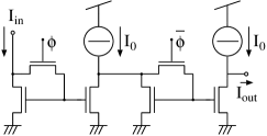
Figure 6: The cascade of two S/H stages aims at signal independent error compensation, however signal dependent errors still add up.

The correct approach to improve the implementation of chaotic maps is to adopt S/H topologies which reduce signal dependent S/H errors. The results presented in this contribution suggest that whenever the speed bottleneck is given by the S/H stages due to the accuracy/sample-latency tradeoff, the operating frequency limit might be pushed forward by adopting such S/H topologies. Examples are offered by differential circuits [6], figure 7 or by the S²I approach [7].

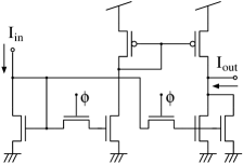
Figure 7: Differential S/H topologies can achieve signal dependent error compensation. For better performance left-hand switch should be twice as long as right-hand one and same width.

References

- [1] M. Delgado-Restituto, F. Medeiro, and A. Rodr guez-V zquez, “Nonlinear, switched current CMOS IC for random signal generation,” Electronic Letters, no. 25, pp. 2190–2191, 1993.
- [2] P. J. Langlois, G. Bergmann, and J. Bean, “A current mode tent map with electrically controllable skew for chaos applications,” in Proceedings of NDES, (Dublin), 1995.
- [3] S. Callegari, G. Setti, and P. J. Langlois, “A CMOS tailed tent map for the generation of uniformly distributed chaotic sequences,” in ISCAS97 proceedings, vol. 2, (Hong Kong), p. 781, June 1997.
- [4] M. Hasler, “Syncronization principles and applications,” in Proceedings of the IEEE ISCAS (Tutorials), (London), pp. 314–327, May 1994.
- [5] T. G. Clarkson, C. K. Ng, and J. Bean, “Review of hardware pRAMs,” in Proceedings of WNNW’93, (York), pp. 18–23, Apr. 1993.
- [6] T. S. Fiez, G. Liang, and D. J. Allstot, “Switched-current circuit design issues,” IEEE Journal of Solid State Circuits, vol. 26, pp. 192–201, Mar. 1991.
- [7] J. B. Hughes and K. W. Moulding, “Enhanced S2I switched-current cells,” in Proc. of ISCAS’96, vol. 1, pp. 187–190, 1996.