Matching-centrality decomposition and the forecasting of new links in networks

Networks play a prominent role in the study of complex systems of interacting entities in biology, sociology, and economics. Despite this diversity, we demonstrate here that a statistical model decomposing networks into matching and centrality components provides a comprehensive and unifying quantification of their architecture. First we show, for a diverse set of networks, that this decomposition provides an extremely tight fit to observed networks. Consequently, the model allows very accurate prediction of missing links in partially known networks. Second, when node characteristics are known, we show how the matching-centrality decomposition can be related to this external information. Consequently, it offers a simple and versatile tool to explore how node characteristics explain network architecture. Finally, we demonstrate the efficiency and flexibility of the model to forecast the links that a novel node would create if it were to join an existing network.

Introduction

The modern world is an increasingly connected place, through transport, social and economic networks, and via our knowledge of interactions at the ecological or molecular level [1, 2, 3]. It is increasingly recognized that such systems should be studied globally, and networks of interacting entities provide a powerful representation of their structure and function. Research on network theory parallels this growth [3]. A first body of research concentrates on the fact that observed networks are often considered to be only partially known. This would be the case in a food web, for instance, in which some real interactions may have yet to be observed, or a protein interaction network where not all pairwise combinations had been tested in the laboratory. Thus, observed links are typically considered as certain, while an absence of a link between a pair of nodes may reflect an absence of information rather than a real absence of interaction. Models have been devised to predict these “missing links ”and thus correct a network dataset for this incomplete sampling or direct future research towards these candidate interactions [4, 5].

A second domain aims to determine if the structure of these networks exhibits basic generalities, and to uncover the processes that may generate these patterns. This aspect has been tackled with a variety of mostly comparative approaches, such as those treating the classification of networks [6, 7], motifs [8], or stochastic models [9]. Progress in this undertaking could be achieved if there were general methods to relate network structure to characteristics of the nodes. For example, body size has been related to patterns in food webs [10], or country politics and trade to the organisation of military conflict networks [11].

A third potential application of research is network forecasting, which would make network theory a predictive science. Many current issues facing human society would benefit from the ability to forecast networks for new nodes joining them, such as for the ecological interactions of invasive species [12], the molecular interactions of a newly discovered protein [13], or the links of a subversive social group [14]. However, there exists no general framework for this forecasting. Here we provide a general model that can be applied to all three domains of network research.

The key feature of our methodology is the development of a model for the probability of interaction between nodes based on the decomposition of network architecture into matching and centrality terms. The matching term quantifies assortative structure in who makes links with whom [15, 16], while the centrality term captures variation in the number of links that nodes make. Typically, research on network structure has focused on patterns in either assortativeness or centrality. However, the architecture of empirical networks is usually a product of both features simultaneously (see e.g. Fortuna et al. [17]). Here, we take into consideration both patterns. Specifically, the decomposition is implemented at the node level, with each node characterized by latent traits of matching and centrality. Latent traits are variables whose values are unknown a priori, but can be estimated a posteriori from the network adjacency matrix itself [18, 19]. The model, called the matching-centrality model, is implemented in such a way that the closer the matching traits of two nodes, the greater the probability that they are linked, and the higher the centrality trait of a node, the greater the probability that this node makes links.

First, based on a dataset of seven networks from disparate fields, we find that this decomposition provides a very precise fit to observed networks. As a result, the model can be used to very accurately predict missing links, as we demonstrate for a terrorist association network. Second, we show that the latent traits of matching and centrality are not just abstract traits, but can be linked to external information about the nodes and thus provide a means to study network organisation. For example, in an ecological network of trophic interactions, the latent traits are related to the body size and the phylogeny of the interacting species. Finally, by placing latent traits as intermediates between the network structure and the characteristics of the nodes, the model offers the possibility to forecast the interactions made by novel nodes when joining the network. For example, in a spatial network of mammal communities on mountains, we show that we can accurately predict the mammal fauna of unsampled mountains based on geographical characteristics.

Results

The matching-centrality model

The model is formulated for undirected bipartite networks, but can be applied to any kind of undirected or directed network, as explained below. Bipartite networks are made of two sets of nodes ($S_{1}$ and $S_{2}$) with connections only between them and not within; plant-pollinator networks provide a classical example. Let be the adjacency matrix of the network, i.e., $a_{ij}=1$ if there is a link between nodes $i$ and $j$, and zero otherwise. The model characterises each node $i$ in set $S_{1}$ by a latent trait of centrality denoted $v_{i}^{*}$, and by $d\geq 1$ latent traits of matching [15, 16] denoted $v_{i}^{1},\dots,v_{i}^{d}$, and similarly, each node $j$ in set $S_{2}$ by a centrality trait $f_{j}^{*}$ and matching traits $f_{j}^{1},\dots,f_{j}^{d}$. The value of $d$ gives the number of matching space dimensions and can be tuned to improve the goodness-of-fit of the model. We take a statistical approach, in which the probability of existence of a link between a pair of nodes $i$ and $j$ (hereafter the linking probability $P(a_{ij}=1)$ is modelled through its logit [20]. Our model is given by

$$\log\left(\frac{P(a_{ij}=1)}{1-P(a_{ij}=1)}\right)=\underbrace{-\sum_{k=1}^{d}\lambda_{k}(v_{i}^{k}-f_{j}^{k})^{2}}_{\text{matching term}}+\underbrace{\delta_{1}v_{i}^{*}+\delta_{2}f_{j}^{*}}_{\text{centrality term }}+m$$ (1)

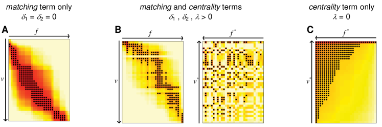
Figure 1: The matching-centrality model. The probability of a link between two nodes is decomposed into a matching term, quantifying assortative structure in who makes links with whom (A), and a centrality term, capturing the fact that nodes can vary considerably in their degree (C). The aim is to simultaneously quantify latent traits of the nodes that are responsible for the matching (v, f) and the centrality (v*, f*) in the network (B). Panels A, B and C show adjacency matrices of three simulated networks, where a black dot represents a link and colors, from yellow to red, represent increasing linking probability computed with the model. The nodes of the matrices are ordered according to their matching or centrality traits. If a network exhibits a modular structure [35, 36, 3], this will be captured by the formation of clusters in the matching traits, while variation in node degree [37, 9, 38, 3] is captured by the centrality traits.

where $\delta_{1},\delta_{2},\lambda_{1},\dots,\lambda_{d}$ are positive constants that scale the relative importance of the matching and centrality terms and $m$ the common intercept (Methods). For a given dimension $d$, the model parameters and latent trait values for each node can be estimated using a simulated annealing algorithm (Methods). Fig. 1 depicts patterns in interaction networks that the model is able to capture. Application to other types of network requires simple modifications: for directed unipartite networks (e.g., food-web or military conflict networks) the two sets of nodes are identical ($S_{1}=S_{2}$); for undirected unipartite networks like most social networks, the adjacency matrix is symmetric, so we have to impose $v_{i}^{k}=f_{i}^{k}$ , $v_{i}^{*}=f_{i}^{*}$, $\delta_{1}=\delta_{2}$ and also that the probability of a self-link is equal to zero ($P(a_{ii}=1)=0$); for more complex networks like directed or undirected multipartite networks, linking probabilities must be set to 0 for pairs of nodes that, by definition, cannot be linked.

Performance of the model

We illustrate the ability of the matching-centrality model to capture network architecture on a set of seven examples from disparate fields (described further in the SI): social interactions in Zachary’s karate club network [21], associations between the terrorists involved in the September 11 attacks [14], military conflicts between countries [11], protein interactions in Saccharomyces cerevisiae [2], the food web of Tuesday Lake [22], the mutualistic seed-dispersal web of Nava de las Correhuelas [23], and presence-absence data of mammal species on peaks within the southern Rocky Mountains [24]. We fit the model for one and two dimensions of matching traits and calculate the AUC, i.e., the area under the receiver operating characteristic (ROC) curve [20]. The AUC is a standard measure of the performance of a classifier, which can be interpreted as the probability that the linking-probability of a true positive is higher than the linking-probability of a true negative (AUC = 0.5 for a random classifier, and 1 for a perfect classifier). Our results yield, for one matching dimension ($d=1$), AUC values falling between $0.9702$ and $0.9967$ and between $0.9977$ and $1$ for $d=2$, three networks being fitted perfectly (Table S1). The ability of the matching-centrality model to capture network architecture is thus high.

Exploring networks using the matching and centrality traits

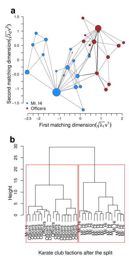
Figure 2: Panel a shows the two-dimensional matching traits space representation of Zachary’s karate-club network [21]. The size of the nodes (club members linked by friendship) is proportional to their centrality trait value. The nodes are displayed in blue or red representing the factions after the split of the club around two members with high centrality. Pannel b shows the Ward’s clustering of the nodes based on the matching and centrality traits.

Once fitted, the model provides a new representation of the network in the latent trait space (Fig. 2, Fig. S2-S7). For example, the plot of the Zachary karate club network (Fig. 2a), which describe the friendship between the 34 members of a university karate club in the period 1970-1972, exhibits two members that have high centrality and divergent matching traits. Shortly after the observations, there was an internal dispute and the club split into two factions, denoted “Mr. Hi ”and “Officers ”. The latent traits could have been used to predict the fault line of this fission: the two groups that formed around these two members can be predicted almost perfectly. The Ward’s hierarchical clustering, based on the matching and centrality traits, clearly shows two distinct groups (Fig. 2b), which matches almost perfectly (except for one member) the factions formed when the club split after the dispute (Methods).

Prediction of missing links in partially known networks

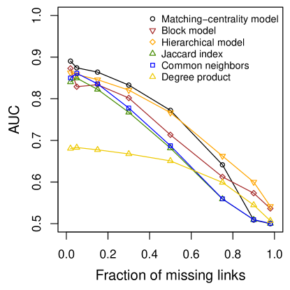
Figure 3: Prediction of missing links in a partially known network. We present the performance of the matching-centrality model (with one dimension) in predicting missing links for the terrorist association network [14], and compare it to several alternative methods [4, 5]. The average AUC statistic (the probability that a missing link is given a higher linking probability than a true negative) is represented as a function of the fraction of simulated missing links created by deleting links in the observed network.

In addition to the exploration of network structure, the matching-centrality model can be used for the prediction of “missing ”links in partially known networks, where the absence of an interaction may in fact reflect an absence of information [25, 4, 5]. Here we demonstrate its performance by simulating missing links in the terrorist association network [14], by setting to 0 a given percentage of links and attempting to recover them (Methods). In the case of this simulation we can judge performance based on the AUC criterion, as the probability that a deleted link is given a higher linking probability than a real absence. For this example, the matching-centrality model outperforms other methods [25, 4, 5] in recovering these deleted links (Fig. 3). However, when more than $50\%$ of the information is missing, the hierarchical decomposition [4] is more precise. This pattern can be explained by the fact that, with a low fraction of observed links, our model tends to overfit the remaining network, and thus underestimates the linking probability for missing links. In practical applications, the absent links with the highest predicted linking probability would be considered to be missing links. These are the candidate interactions that should come under the scrutiny of researchers, thus serving as a guide for cost-effective analysis of complex systems. Unlike previous methods [4, 5], our approach is not limited to undirected networks.

Linking latent traits and node characteristics

As shown above, the model can be fitted and used for prediction simply based on the network itself. However, it also offers an intuitive tool to gain insight into the processes underlying network structure, as the matching and centrality traits of nodes can be related to independent information about them using standard analyses such as linear models or Mantel tests. In the food web of Tuesday Lake [22, 26], both the matching and centrality traits of predators and prey are related to their body size and phylogeny (Methods, Table S2). The latent traits are thus not just an abstract characterisation of the nodes, but provide a versatile method to unravel factors underlying the different aspects of network structure.

Forecasting the links of new nodes

Finally, a significant feature of the matching-centrality model is the possibility to forecast the links that new nodes would create when joining an existing network. This might be applied, for example, to forecast the interactions of an invasive species entering a food web or pollination network, the contacts of a non-surveyed individual in a terrorist network, or the biota of an unsampled mountain. The procedure is as follows: from the adjacency matrix we first estimate the latent traits of matching and centrality for each node in the existing network, and verify that our model provides an accurate fit. Then, using appropriate statistical models, we relate the latent traits of the nodes to external information about them, and ensure that the latter provides a good predictive power for the former. If both conditions are met, we can predict the matching and centrality traits of the new node(s) using the external information, and finally their linking probability with each of the existing nodes.

We illustrate the method using the network describing the presence-absence of mammal species on mountains within the Rocky Mountains [24]. The model fits this network perfectly, with an AUC for two matching dimension of $1$. Furthermore, we find that the estimated matching and centrality traits of the mountains are closely related to their geographical characteristics. Specifically, using a generalized least square linear model with a spatial correlation structure, we can relate the latent traits of matching and centrality to the area, elevation, and geographic position of the mountains (equation (6), Methods, Table S3). Once the model fitted, it is possible to estimate the traits of matching and centrality for an unsampled mountain based on its geography. Here, because of the correlation structure, the estimation of the latent traits is based on the conditional expectation of a multivariate normal distribution (equation (8) and (9), Methods). The predicted matching and centrality traits are then used in the matching-centrality model (equation (1)) to estimate the linking probabilities for each mammal species with the unsampled mountain. We demonstrate the capacity of the model by simulation, removing a single mountain or a set of four, and attempting to forecast the mammal fauna. The model performs remarkably well: on average $87\%$ of the data are correctly forecasted (Fig. 4). It must, however, be kept in mind that the applicability of the method depends on the conditions that 1) the matching-centrality model fits the network closely, 2) that external information on the nodes can accurately predict the latent traits, and 3) that the nodes to be forecasted must belong to the same statistical population as the observed ones. In all cases, we recommend out-of-sample tests, as explained in the Methods.

To our knowledge, only one other method has been devised to forecast the links made by a new node in a network, for a host-parasitoid network based on the phylogenies of the participants [27]. Our approach has two decisive advantages that make it extremely versatile: firstly, it is not necessary to include information about both sets of nodes of the bipartite network to make the forecast; secondly, by placing latent traits as intermediates between the network adjacency matrix and node characteristics, we provide an entirely flexible way to incorporate external information about nodes, for any conceivable statistical model could be used to relate the latent traits to external variables. Both features are illustrated in the above example, where the forecasting is based only on information about the mountains, and the missing latent traits are estimated from the geographic characteristics using linear predictors and spatial correlation.

Discussion

By translating an adjacency matrix into a set of quantitative traits for the nodes, the matching-centrality model represents a powerful and unifying tool for network analysis. It allows the reconstruction of missing information and the forecasting of the links of entirely novel nodes, and opens the door to comparative analyses to shed light on the factors underlying network structure across disciplines.

Materials and Methods

Fitting of the model
The likelihood of the model is computed by

$$L=\prod_{ij}P(a_{ij}=1)^{a_{ij}}(1-P(a_{ij}=1))^{(1-a_{ij})}$$ (2)

i.e., we assume the presence-absence of links follows a multi-Bernoulli distribution and that the probabilities are independent given the parameters and the latent traits. As the logit of the linking probabilities is a non-linear function of the parameters, we fit the model using a simulated annealing algorithm [28].

In order to make the parameters and the latent traits of the model uniquely defined we have to impose some constraints:

1. All vectors of latent traits $\vec{v^{k}},\vec{f^{k}},\vec{v^{*}},\text{and}\vec{f^{*}}$ are orthogonal to the unitary vector.

2. All vector of matching trait $\vec{v^{k}}$ ($k=1,\cdots,d$) are pair-wise orthogonal, and the same for the vectors $\vec{f^{k}}$.

3. The length of the vectors $\vec{v^{k}},\vec{v^{*}}$ is set to $\sqrt{(\#S_{1})}$, where $\#S_{1}$ is the number of node in set $S_{1}$. Similarly for the set $S_{2}$, the length of the vectors $\vec{f^{k}},\vec{f^{*}}$ is set to $\sqrt{(\#S_{2})}$.

Nodes clustering base on the latent traits Using the estimated values of the latent traits of matching and centrality, we can construct a dendrogram using the following distance $d_{ij}$ between two nodes $i$ and $j$:

$$d_{ij}=\frac{\sqrt{\lambda_{1}(v_{i}^{1}-v_{j}^{1})^{2}+\lambda_{2}(v_{i}^{2}-v_{j}^{2})^{2}}}{\delta v_{i}^{*}+\delta v_{j}^{*}-2min_{k}(\delta v_{k}^{*})}$$ (3)

with the parameters coming from the model (equation (1)). Note that the numerator is the classical Euclidian distance in a two dimensional matching trait space; the denominator is a correction term that weights distances according to the centrality of the nodes $i$ and $j$ compared to the minimum centrality of the $k$ nodes in the network. The greater the value of the centrality trait of a node, the greater the “compression” of the distances; this reflects the fact that the probability of attachment is proportional to the degree of a node (captured by the centrality term).

Predicting missing links in partially know networks
We used the terrorist association network [14] to evaluate the performance of the matching-centrality model to recover missing links. We followed the same procedure as in Clauset et al. [4]. Specifically, we simulated networks with missing links by setting a given fraction of 1s to 0s in the adjacency matrix. Then the model is fitted to the incompletely observed networks and latent traits estimated for each node. These matching and centrality traits are then used to estimate linking probabilities for each pair of nodes (equation 1). Finally we computed the AUC for the 0’s and the missing links pooled. We removed at random 2, 5, 15, 30, 50, 75, 90 and 98% of the 1’s, replicated 100 times for each fraction. For comparison, we present results with the hierarchical model of Clauset et al. [4], block model of Guimera et al. [5], and three classical techniques [25] (Jaccard index, Common neighbors, Degree product).

Linking latent traits and node characteristics
We used phylogenetic regression [29] to relate the latent traits of matching and centrality to species’ body-size and phylogeny in the food-web of Tuesday lake. We assume that the latent traits follow a multivariate normal distribution (MVN), where the linear term is given by the logarithm of the body-size and the correlation structure is induced by the phylogeny, i.e.,

$$\vec{v^{1}},\vec{v^{2}},\vec{f^{1}},\vec{f^{2}},\vec{v^{*}},\vec{f^{*}}\sim MVN\left(\alpha+\beta\log(\vec{bs}),\Sigma(\Lambda)\right)$$ (4)

where: $\vec{v^{1}},\vec{v^{2}},\vec{f^{1}},\vec{f^{2}},\vec{v^{*}},\vec{f^{*}},\vec{bs}$ denote the vectors of the matching traits of resources and consumers, the centrality traits of resources and consumers, and the body-sizes, respectively; $\Sigma(\Lambda)$ is the variance-covariance matrix; and $\alpha,\beta$ and $\lambda$ are the parameters of the phylogenetic regression. We use Pagel’s-$\lambda$ [30] structure for the variance-covariance matrix, i.e.,

$$\Sigma(\lambda)_{ij}=\left\{\begin{array}[]{ccc}\sigma^{2}\cdot t_{ij}\cdot\lambda&\text{if}&i\neq j\\ \sigma^{2}&\text{if}&i\neq j\end{array}\right.$$ (5)

where $\sigma^{2}$ is the common variance, $t_{ij}$ is the proportion of time that species $i$ and $j$ spent in common before their speciation on the phylogenetic tree, and  is the control parameter for the strength of the phylogenetic correlation ($\lambda=0$ is equivalent to no correlation). The p-values of the parameters $\alpha$ and $\beta$ are computed with the usual z-test, while the p-value associated with the correlation structure is computed using a log-likelihood ratio test between models with and without correlation. The analyses were done in R [31] with the libraries ape [32] and nlme [33].

Forecasting the links of new nodes
The analyses of the latent traits for the mountains were carried out using generalized least squares regression with a spatial correlation structure [34]. We assume that the matching and centrality traits follow a multivariate normal distribution, where the linear part is given by the longitude, latitude, area and elevation of the mountains, and that the spatial correlation structure is exponential, i.e.,

$$\vec{v^{1}},\vec{v^{2}},\vec{v^{*}}\sim MVN(\alpha+\beta_{1}\cdot\text{area}+\beta_{2}\cdot\text{elevation}+\beta_{3}\cdot\text{latitude}+\beta_{4}\cdot\text{longitude},\Sigma(r)),$$ (6)

with the elements of the variance-covariance matrix given by

$$\Sigma(r)_{kl}=\sigma^{2}e^{-d_{kj}/r}.$$ (7)

The vectors $\vec{v^{1}},\vec{v^{2}},\vec{v^{*}}$ are the matching and centrality traits, respectively; $\alpha,\beta_{1},\beta_{2},\beta_{3},\beta_{4}$ are the intercept and slope parameters; $r$ is a parameter tuning the exponential decay of the spatial correlation; $\sigma$ common variance; and $d_{ij}$ the distance between mountains $i$ and $j$. For the matching traits, we found that only the spatial correlation structure was significant (table S3). For the centrality traits, all covariates except the longitude and the correlation structure were significant.

Since the matching and centrality traits of the mountains are significantly related to several covariates and to the correlation structure given by the between-mountain distances, it should be possible to forecast the mammal communities in unsampled mountains for which the covariates are known, given the information provided by the covariates of the sampled mountains and the observed presence/absence network.

To achieve this task, the first stage is to check that the matching and centrality traits of the sampled mountains can be recovered from the covariates. If this ability exists, using the model for forecasting is then reasonable. In the first stage, we use conditional expectation to test if there is sufficient predictive power to recover the matching and centrality traits of the mountains. This out-of-sample test is carried out in the following three steps:

1. We refit the model (6) on the data set after removing one mountain, denoted by $k$.

2. Using the fitted parameters from step 1), we compute the conditional expectation for the matching and centrality traits of mountain $k$; for the centrality trait, this value is given by:

   $$\hat{v_{k}^{*}}=\hat{\alpha}+\hat{\beta_{1}}\cdot\text{area}+\hat{\beta_{2}}\cdot\text{elevation}+\hat{\beta_{3}}\cdot\text{latitude}$$ (8)

   where $\hat{\alpha},\hat{\beta_{1}},\hat{\beta_{2}},\hat{\beta_{3}},\hat{r}$ are the fitted parameters from step 1). The conditional expectation for the matching trait is given by:

   $$\hat{v_{k}}=\hat{\alpha}+\Sigma(\hat{r})_{-kk}\Sigma(\hat{r})^{-1}_{kk}\left(\vec{v_{-k}}-\hat{v_{-k}}\right),$$ (9)

   where $\Sigma(\hat{r})_{-kk}$ is the $k$th column without the $k$th row (indicated by subscript $-k$) of the variance-covariance matrix estimated using equation 7; $\Sigma(\hat{r})_{kk}$ is the $(k,k)$ element of the estimated variance-covariance matrix; $\left(\vec{v_{-k}}-\hat{v_{-k}}\right)$ is the row vector of residuals obtained from step 1. The last term of equation (9) represents the deviation from the linear prediction that is introduced by knowledge of the spatial correlation structure. Note that only the spatial correlation and the intercept are significant for the matching trait (table S3).

3. We repeat steps 1 and 2 for all mountains in turn and then finally compare the predicted values of matching and centrality and the observed values (the values estimated from the matching-centrality model fitted to the full network) with a simple linear correlation coefficient.

We found a correlation of $0.95$ for the centrality traits, and of $0.71$ and $0.62$ for the two dimensions of matching traits. Our model thus has a good predictive power to recover the latent traits of the mountains. This result opens the door to the forecasting of the presence/absence of mammal species on mountains that have not been sampled, but for which we know their characteristics (area, elevation, latitude and distances to the other mountains). In this second stage, we test the forecasting performance of the matching-centrality model by removing each mountain from the dataset in turn and attempting to recover its mammal community. This yields the following out-of-sample test:

1. We remove one mountain from the network, and then estimate the matching and centrality traits of the mammals and of the remaining mountains using the matching-centrality model.

2. Based on the model (equation (6)) and on the conditional expectation (equations (8) and (9)), we predict the matching and centrality traits for the removed mountain.

3. With the predicted matching and centrality traits, we can predict the linking probabilities (equation 1) between the removed mountain and the mammals. The presence/absence of the mammals are determined from these linking probabilities and the cut-off point obtained with the fit of step 1. The cut-off point is defined as the linking probability chosen such that the number of false positives is equal to the number of false negatives.

In a real case situation for the forecasting of unsampled nodes, the first condition for application is that the matching-centrality model provides a good fit to the sampled network. Secondly, there must exist a relationship between the matching and centrality traits and the independent information on the nodes; in our example, forecasting the mountains occupied by a new mammal would not be possible. Thirdly, it is necessary that the first stage described above is successful, in our case that the matching and centrality traits of the sampled mountains can be recovered from the covariates, for otherwise we can have little faith in the results of forecasting. Once these conditions are met, one can proceed to the forecasting of the edges connected to the unsampled nodes. This is performed with steps 2 and 3 of the second stage.

We note three final technical points. Firstly, we recommend the performance of a complete out-of-sample test (steps 1 to 3 of the second stage) as additional validation. Secondly, the new nodes have to belong to the same statistical population as the original ones (it would obviously make no sense to forecast the mammal community present in a completely different region). Thirdly, in our example, we related the matching and centrality traits to the characteristics of the nodes using linear models; our approach is versatile and models of any form can be applied at this stage.

ACKNOWLEDGMENTS We thank J. Bascompte, S. Saavedra, and A. Davison for critical discussion. The work was funded by the National Centre of Competence in Research ”Plant Survival”, the Swiss National Science Foundation grant 3100A0-113843 (both to L.-F. Bersier), by SystemsX.ch, the Swiss Initiative in Systems Biology (to L.-F. Bersier and C. Mazza), and by the FP7-REGPOT-2010-1 program (project 264125 EcoGenes) and an ERC Advanced Grant (both to J. Bascompte).

Figure 4: Performance of thematching-centrality model in forecasting the mammal communities on unsampled mountains. We illustrate the performance of the model using an out-of-sample test, removing singly and in groups of four each mountain in the network [24]. After fitting the model to the known network, we use a statistical analysis to predict the latent traits of the unsampled mountains from geographical characteristics, and use these traits in thematching-centrality model to forecast their mammal community. Graphs show box-plots for the AUC and the accuracy of the forecasts (i.e., the percentage of correctly forecasted 0s and 1s).

References

- [1] Cohen, J. E. Food Webs and Niche Space (Princeton University Press, Princeton, New Jersey, 1978).
- [2] Maslov, S. & Sneppen, K. Specificity and stability in topology of protein networks. Science 296, 910–913 (2002).
- [3] Newman, M. E. J. Networks: An Introduction (Oxford University Press, Oxford, 2010).
- [4] Clauset, A., Moore, C. & Newman, M. E. J. Hierarchical structure and the prediction of missing links in networks. Nature 453, 98–101 (2008).
- [5] Guimera, R. & Sales-Pardo, M. Missing and spurious interactions and the reconstruction of complex networks. Proc. Natl. Acad. Sci. U.S.A. 106, 22073–22078 (2009).
- [6] Guimera, R., Sales-Pardo, M. & Amaral, L. A. N. Classes of complex networks defined by role-to-role connectivity profiles. Nature Phys. 3, 63–69 (2007).
- [7] Onnela, J.-P. et al. Taxonomies of networks from community structure. Phys. Rev. E 86 (2012).
- [8] Milo, R. et al. Network motifs: Simple building blocks of complex networks. Science 298, 824–827 (2002).
- [9] Barabasi, A. L. & Albert, R. Emergence of scaling in random networks. Science 286, 509–512 (1999).
- [10] Petchey, O. L., Beckerman, A. P., Riede, J. O. & Warren, P. H. Size, foraging, and food web structure. Proc. Natl. Acad. Sci. U.S.A. 105, 4191–4196 (2008).
- [11] Ward, M. D., Siverson, R. M. & Cao, X. Disputes, democracies, and dependencies: A reexamination of the kantian peace. Am. J. Polit. Sci. 51, 583–601 (2007).
- [12] Memmott, J. Food webs: a ladder for picking strawberries or a practical tool for practical problems? Phil. Trans. R. Soc. B 364, 1693–1699 (2009).
- [13] Garcia-Garcia, J. et al. Networks of protein-protein interactions: From uncertainty to molecular details. Mol. Inf. 31, 342–362 (2012).
- [14] Krebs, V. E. Mapping networks of terrorist cells. Connections 24, 43–52 (2002).
- [15] Rossberg, A. G., Matsuda, H., Amemiya, T. & Itoh, K. Food webs: Experts consuming families of experts. J. Theor. Biol. 241, 552–563 (2006).
- [16] Rossberg, A. G., Brannstrom, A. & Dieckmann, U. How trophic interaction strength depends on traits. Theor. Ecol. 3, 13–24 (2010).
- [17] Fortuna, M. A., Popa-Lisseanu, G., Ibanez, C. & Bascompte, J. The roosting spatial network of a bird-predator bat. Ecology 90, 934–944 (2009).
- [18] Hoff, P. D., Raftery, A. E. & Handcock, M. S. Latent space approaches to social network analysis. J. Amer. Statist. Assoc. 97, 1090–1098 (2002).
- [19] Rohr, R., Scherer, H., Kehrli, P., Mazza, C. & Bersier, L. Modeling food webs: exploring unexplained structure using latent traits. Am. Nat. 173, 170–177 (2010).
- [20] Kolaczyk, E. Statistical Analysis of Network Data (Springer, New York, 2009).
- [21] Zachary, W. W. An information flow model for conflict and fission in small groups. J. Anthrop.l Res. 33, 452–473 (1977).
- [22] Jonsson, T., Cohen, J. E. & Carpenter, S. R. Food webs, body size, and species abundance in ecological community description. In Caswell, H. (ed.) Adv. Ecol. Res., Vol 36, 1–84 (Elsevier Academic Press, 2005).
- [23] Rezende, E. L., Lavabre, J. E., Guimaraes, P. R., Jordano, P. & Bascompte, J. Non-random coextinctions in phylogenetically structured mutualistic networks. Nature 448, 925–928 (2007).
- [24] Patterson, B. D. Mammalian extinction and biogeography in the southern rocky mountains. In Nitecki, M. H. (ed.) Extinctions, 247–293 (The University of Chicago Press, Chicago, 1984).
- [25] Liben-Nowell, D. & Kleinberg, J. The link-prediction problem for social networks. J. Assn. Inf. Sci. Technol. 58, 1019–1031 (2007).
- [26] Naisbit, R. E., Rohr, R. P., Rossberg, A. G., Kehrli, P. & Bersier, L.-F. Phylogeny versus body size as determinants of food web structure. Proc. R. Soc. B 279, 3291–3297 (2012).
- [27] Ives, A. R. & Godfray, H. C. J. Phylogenetic analysis of trophic associations. Am. Nat. 168, E1–E14 (2006).
- [28] Brémaud, P. Markov chains, gibbs fields, monte carlo simulation, and queues (1998).
- [29] Grafen, A. The phylogenetic regression 326, 119–157 (1989).
- [30] Freckleton, R. P., Harvey, P. H. & Pagel, M. Phylogenetic analysis and comparative data: A test and review of evidence. Am. Nat. 160, 712–726 (2002).
- [31] Team, R. D. C. R: A language and environment for statistical computing (R Foundation for Statistical Computing, Vienna, Austria, 2009).
- [32] Paradis, E., Claude, J. & Strimmer, K. Ape: Analyses of phylogenetics and evolution in r language. Bioinformatics 20, 289–290 (2004).
- [33] Pinheiro, J., Bates, D., DebRoy, S., Sarkar, D. & team, R. C. nlme: Linear and nonlinear mixed effects models (2009).
- [34] Zuur, A. F., Ieno, E. N., Walker, N. J., Saveliev, A. A. & Smith, G. M. Mixed Effects Models and Extensions in Ecology with R (Springer, 2009).
- [35] Melian, C. J. & Bascompte, J. Food web cohesion. Ecology 85, 352–358 (2004).
- [36] Newman, M. E. J. & Girvan, M. Finding and evaluating community structure in networks. Phys. Rev. E 69, 1–15 (2004).
- [37] Price, D. J. D. Networks of scientific papers. Science 149, 510–515 (1965).
- [38] Amaral, L. A. N., Scala, A., Barthelemy, M. & Stanley, H. E. Classes of small-world networks. Proc. Natl. Acad. Sci. U.S.A. 97, 11149–11152 (2000).