Spectral projections of the complex cubic oscillator

Abstract

We prove the spectral instability of the complex cubic oscillator $-\frac{d^{2}}{dx^{2}}+ix^{3}+i\alpha x$ for non-negative values of the parameter $\alpha$, by getting the exponential growth rate of $\|\Pi_{n}(\alpha)\|$, where $\Pi_{n}(\alpha)$ is the spectral projection associated with the $n$-th eigenvalue of the operator. More precisely, we show that for all non-negative $\alpha$

$$\lim\limits_{n\to+\infty}\frac{1}{n}\log\|\Pi_{n}(\alpha)\|=\frac{\pi}{\sqrt{3}}.$$

Keywords: non-selfadjoint operators, complex WKB estimates.

1 Introduction

We consider the complex cubic oscillator

$${\mathcal{A}}_{\alpha}=-\frac{d^{2}}{dx^{2}}+ix^{3}+i\alpha x,\leavevmode\nobreak\ \leavevmode\nobreak\ \alpha\in\mathbb{R}$$ (1.1)

on the real line. We define ${\mathcal{A}}_{\alpha}$ by extension of the operator

$${\mathcal{A}}_{\alpha}^{0}=-\frac{d^{2}}{dx^{2}}+ix^{3}+i\alpha x,\leavevmode\nobreak\ \leavevmode\nobreak\ \leavevmode\nobreak\ \leavevmode\nobreak\ \leavevmode\nobreak\ {\mathcal{D}}({\mathcal{A}}_{\alpha}^{0})=\mathcal{C}_{0}^{\infty}(\mathbb{R}),$$

which is accretive, so we can define ${\mathcal{A}}_{\alpha}:=\overline{{\mathcal{A}}_{\alpha}^{0}}$ as its closure. ${\mathcal{A}}_{\alpha}$ is then maximally accretive, with domain

$${\mathcal{D}}({\mathcal{A}}_{\alpha})=H^{2}(\mathbb{R})\cap L^{2}(\mathbb{R};x^{6}dx).$$

The cubic oscillator presented here has been studied in [11] and [21]. It also belongs to the class of operators considered in [19]. Let us mention [14] as well, which deals with a quadratic perturbation of the cubic $ix^{3}$ potential.
The operator ${\mathcal{A}}_{\alpha}$ has compact resolvent, and its eigenvalues $(\lambda_{n}(\alpha))_{n\geq 1}$ are simple in the sense of the geometric multiplicity.
The properties of the complex cubic oscillator and its variants (the potential $x^{2}+ix^{3}$, for instance), have been widely studied in the past few years (see [3, 4, 5, 6, 9, 10, 11, 14, 16, 21, 22, 19]). As a non-selfadjoint operator, it has a surprising property: its spectrum is purely real for $\alpha\geq 0$ (see [4] for numerical observations and [19] for a rigorous proof). This property is suspected to be related with the so-called $\mathcal{PT}$-symmetry of the operator, namely

$$\mathcal{PT}{\mathcal{A}}_{\alpha}={\mathcal{A}}_{\alpha}\mathcal{PT},$$

where $\mathcal{P}$ and $\mathcal{T}$, denoting respectively the spatial symmetry and time inversion operators, act as follows:

$$({\mathcal{P}}u)(x)=u(-x)\leavevmode\nobreak\ \leavevmode\nobreak\ \leavevmode\nobreak\ \textrm{ and }\leavevmode\nobreak\ \leavevmode\nobreak\ \leavevmode\nobreak\ (\mathcal{T}u)(x)=\overline{u(x)}.$$

The complex cubic oscillator is a toy model in the study of $\mathcal{PT}$-symmetric operators.
One of the main questions arising from this property of real spectrum is the following: does ${\mathcal{A}}_{\alpha}$ share some other similarities with selfadjoint operators? More precisely, does the family of eigenfunctions form a basis of $L^{2}(\mathbb{R})$ in some sense? Is the spectrum stable under perturbations of the operator? What can one say about the behavior of the eigenvalues for negative values of $\alpha$? Some of these questions have already been answered, while other have been stated as conjectures. For instance, it has been established in [16] that the eigenfunctions of ${\mathcal{A}}_{\alpha}$ do not form a Riesz basis, as well as the existence of non-trivial pseudospectra.
The properties of the spectrum of ${\mathcal{A}}_{\alpha}$ for negative $\alpha$ have not been completely understood yet. Numerical simulations (see [9], [10], [11]), reproduced on Figure 1, suggest that, for any $n\geq 1$, there exists a critical value $\alpha_{n}^{crit}<0$ of the parameter such that $\lambda_{n}(\alpha)$ is real for $\alpha>\alpha_{n}^{crit}$. For $\alpha=\alpha_{n}^{crit}$, $\lambda_{n}(\alpha_{n}^{crit})$ seems to cross an adjacent eigenvalue, forming for $\alpha<\alpha_{n}^{crit}$ a complex conjugate pair lying away from the real axis. Regarding the analysis for large eigenvalues which we will perform in the following, the simulation suggests that, for any fixed $\alpha<0$, the eigenvalues $\lambda_{n}(\alpha)$ are real for $n$ large enough, but it does not seem to be proved yet. Therefore, we will only consider non-negative values of $\alpha$ in the following.

Our goal is to measure the spectral instability of the operator ${\mathcal{A}}_{\alpha}$. As mentioned above, the instability of the eigenvalues $\lambda_{n}(\alpha)$ has already been highlighted in [16] by proving the existence of non-trivial pseudospectra. We now want to understand more accurately this phenomenon, following the approach of [7], [8] and [15].
To this purpose, we define the instability indices

$$\kappa_{n}(\alpha)=\|\Pi_{n}(\alpha)\|,$$ (1.2)

where $\Pi_{n}(\alpha)$ denotes the spectral projection of ${\mathcal{A}}_{\alpha}$ associated with the eigenvalue $\lambda_{n}(\alpha)$ (the eigenvalues being labelled in increasing order). We shall first consider the question of algebraic multiplicity for the eigenvalues $\lambda_{n}(\alpha)$, that is, whether there exist associated Jordan blocks or not. The algebraic simplicity of the eigenvalues has been proved for all $n\geq 1$ in [14] in the case of a potential of the form $ax^{2}+i\sqrt{\beta}x^{3}$. Here, by an independent proof, we shall get the algebraic simplicity of $\lambda_{n}(\alpha)$, but only for $n$ large enough, which will be enough to achieve the proof of our main statement. Hence, for $n$ large enough, the expression

$$\kappa_{n}(\alpha)=\frac{\|u_{n}^{\alpha}\|^{2}}{|\langle u_{n}^{\alpha},\bar{u}_{n}^{\alpha}\rangle|}$$ (1.3)

will hold, where $u_{n}^{\alpha}$ denotes an eigenfunction of ${\mathcal{A}}_{\alpha}$ associated with the eigenvalue $\lambda_{n}(\alpha)$ (see [2]). We will use this formula to prove the following theorem, which is the main statement of our work.

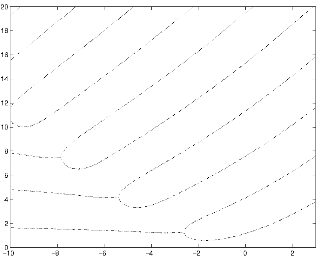
Figure 1: Real parts of the eigenvalues of ${\mathcal{A}}_{\alpha}$ as functions of $\alpha$. Each pair of consecutive eigenvalues becomes non-real, complex conjugate on the left of the branch point.

Theorem 1.1

For all $\alpha\geq 0$, we have

$$\lim\limits_{n\to+\infty}\frac{1}{n}\log\kappa_{n}(\alpha)=\frac{\pi}{\sqrt{3}}.$$ (1.4)

Let us recall that the same question was considered in [7, 8, 15] in the case of anharmonic oscillators $-\frac{d^{2}}{dx^{2}}+e^{i\theta}|x|^{m}$, $m>0$, $|\theta|<\min\{(m+2)\pi/4,(m+2)\pi/2m\}$. More precisely, it has been proved that the spectral projections of these operators grow faster than any power of $n$ as $n\rightarrow\infty$ [7], and the exponential growth rate was precisely obtained for $m=2$ in [8] and for every even exponent $m$ in [15].
The proof of Theorem 1.1 lies on WKB estimates of the eigenfunctions in the complex plane. This method has already been used in [15] in the even anharmonic case. However, here we will have to manage the sub-principal term $i\alpha x$ in the potential.
Some results from [16] can be recovered immediately from Theorem 1.1:

Corollary 1.2

For all $\alpha\geq 0$, the eigenfunctions of ${\mathcal{A}}_{\alpha}$ do not form a Riesz basis.

Proof: Let $(u_{n}^{\alpha})_{n\geq 1}$ be a family of eigenfunctions for ${\mathcal{A}}_{\alpha}$ associated with the eigenvalues $(\lambda_{n}(\alpha))_{n\geq 1}$. Let us recall that $(u_{n}^{\alpha})_{n\geq 1}$ is said to be a Riesz basis if it spans a dense subset of $L^{2}(\mathbb{R})$ and if there exists $C>0$ such that, for all $\phi\in L^{2}(\mathbb{R})$,

$$C^{-1}\sum_{n=1}^{+\infty}|\langle\phi,u_{n}^{\alpha}\rangle|^{2}\leq\|\phi\|^{2}\leq C\sum_{n=1}^{+\infty}|\langle\phi,u_{n}^{\alpha}\rangle|^{2}\,.$$ (1.5)

According to Lemma 3.1 and Proposition 3.2 (which provides algebraic simplicity for large eigenvalues of ${\mathcal{A}}_{\alpha}$), we can choose the eigenfunctions $u_{n}^{\alpha}$ such that, for $n,m\geq 1\,$ and $n$ large enough, $\langle u_{n}^{\alpha},\overline{u_{m}^{\alpha}}\rangle=\delta_{n,m}$. Hence according to (3.1), we have $\kappa_{n}(\alpha)=\|u_{n}^{\alpha}\|^{2}$ for $n$ large enough. Using that $\kappa_{n}(\alpha)\rightarrow+\infty$ as $n\rightarrow+\infty$, it is then straightforward to check that the sequence $\phi_{n}=\overline{u_{n}^{\alpha}}$ can not satisfy (1.5). $\square$
Furthermore, the pseudospectra in the neighborhood of an eigenvalue are known to grow proportionally to the corresponding instability index (see [2], [20]). Hence the exponential growth obtained in Theorem 1.1 enables us to confirm the presence of nontrivial pseudospectra [16], and to somehow describe its shape near the eigenvalues.

Section 2 is devoted to the estimates on the eigenfunctions needed to prove Theorem 1.1. The proof itself is achieved in Section 3.

2 Asymptotic behavior of the eigenfunctions

2.1 Preliminary scale change

Let us first perform the following scale change. Let us recall that for all $\alpha\geq 0$, the spectrum of ${\mathcal{A}}_{\alpha}$ is real, and let us denote the eigenvalues, labelled in increasing order, by $\lambda_{n}(\alpha)$. We set

$$\left\{\begin{array}[]{ccc}h_{n}&=&\lambda_{n}(\alpha)^{-5/6}\\ \tilde{x}&=&h_{n}^{2/5}x.\end{array}\right.$$ (2.1)

The operator $({\mathcal{A}}_{\alpha}-\lambda_{n}(\alpha))$ then writes

$$-h_{n}^{4/5}\frac{d^{2}}{d\tilde{x}^{2}}+ih_{n}^{-6/5}\tilde{x}^{3}+i\alpha h_{n}^{-2/5}\tilde{x}-\lambda_{n}(\alpha)=h_{n}^{-6/5}\left(-h_{n}^{2}\frac{d^{2}}{d\tilde{x}^{2}}+i\tilde{x}^{3}+i\alpha h_{n}^{4/5}\tilde{x}-1\right),$$

and we are reduced to the study of the kernel of

$${\mathcal{A}}_{\alpha}(h)=-h^{2}\frac{d^{2}}{dx^{2}}+ix^{3}+i\alpha h^{4/5}x-1.$$

An eigenfunction $u_{n}^{\alpha}$ of ${\mathcal{A}}_{\alpha}$ associated with $\lambda_{n}(\alpha)$ can be written as

$$u_{n}^{\alpha}(x)=\psi_{\alpha}(h_{n}^{2/5}x,h_{n})=\psi_{\alpha}(\lambda_{n}(\alpha)^{-1/3}x,h_{n}),$$ (2.2)

where $\psi_{\alpha}(\cdot,h_{n})$ is a solution of

$${\mathcal{A}}_{\alpha}(h_{n})\psi_{\alpha}(\cdot,h_{n})=0,\leavevmode\nobreak\ \leavevmode\nobreak\ \leavevmode\nobreak\ \psi_{\alpha}(\cdot,h_{n})\in L^{2}(\mathbb{R}).$$ (2.3)

Notice that the condition $\psi_{\alpha}(\cdot,h_{n})\in L^{2}(\mathbb{R})$, together with (2.3), ensure that $\psi_{\alpha}(\cdot,h_{n})$ belongs to the domain ${\mathcal{D}}({\mathcal{A}}_{\alpha}(h_{n}))={\mathcal{D}}({\mathcal{A}}_{\alpha})$ (see for instance Theorem 2.1 below). Thus, we will now work on these solutions $\psi_{\alpha}$.
From now on, $\alpha$ is assumed to be fixed and non-negative.

2.2 Behavior of the eigenfunctions away from the turning points

In this subsection, we determine the global asymptotic behavior of the solutions $\psi_{\alpha}(x,h)$ of

$${\mathcal{A}}_{\alpha}(h)\psi_{\alpha}(x,h)=0,\leavevmode\nobreak\ \leavevmode\nobreak\ \leavevmode\nobreak\ \psi_{\alpha}(\cdot,h)\in L^{2}(\mathbb{R})$$ (2.4)

as $h\rightarrow 0$.
More precisely, we want to understand the behavior of $\psi_{\alpha}$ in a domain of the complex plane avoiding the zeroes (called turning points of the equation) of the potential

$$V_{\alpha}(x,h)=ix^{3}+i\alpha h^{4/5}x-1.$$

Let $x_{+}^{\alpha}(h)$, $x_{-}^{\alpha}(h)$ and $x_{\mathbf{i}}^{\alpha}(h)$ denote the zeroes of $V_{\alpha}(\cdot,h)$, respectively starting at $h=0$ from the zeroes $x_{+}^{0}=e^{-i\pi/6}$, $x_{-}^{0}=e^{-5i\pi/6}$ and $x_{\mathbf{i}}^{0}=i$ of the potential

$$V_{0}(x)=ix^{3}-1.$$

Note that for $h$ small enough, $x_{\pm}^{\alpha}(h)$, $x_{\mathbf{i}}^{\alpha}(h)$ are simple zeroes of $V_{\alpha}(\cdot,h)$.
To understand the asymptotic properties of the solutions of (2.4), it will be useful to analyze the geometry of the level curves (Stokes lines) of the function

$$x\mapsto{\rm Re\,}\int_{x_{+}^{\alpha}(h)}^{x}\sqrt{V_{\alpha}(z,h)}\leavevmode\nobreak\ dz,$$

where $\sqrt{V_{\alpha}}$ is holomorphic in

$$D_{h}^{\alpha}=\mathbb{C}\setminus\bigcup_{\tiny{\sigma\in\{+,-,\mathbf{i}\}}}\{(1+r)x_{\sigma}^{\alpha}(h):r>0\},$$

and $\sqrt{V_{\alpha}(0,h)}=i$.
The path of integration is included in $D_{h}^{\alpha}$.
Let us notice that $x_{+}^{\alpha}(h)$ and $x_{-}^{\alpha}(h)$ belong to a common, bounded Stokes line, joining the two points:

$${\rm Re\,}\int_{x_{-}^{\alpha}(h)}^{x_{+}^{\alpha}(h)}\sqrt{V_{\alpha}(z,h)}\leavevmode\nobreak\ dz=0.$$

Let us denote this line by $\ell_{f}^{\alpha}(h)$. It is the only bounded Stokes line for ${\mathcal{A}}_{\alpha}$ (see Figure 2).
On the other hand, there are seven unbounded Stokes lines starting from $x_{\pm}^{\alpha}(h)$, $x_{\mathbf{i}}^{\alpha}(h)$, with the five asymptotic directions as $|x|\rightarrow+\infty$,

$$D_{k}=\arg^{-1}\left\{\frac{\pi}{10}+\frac{2k\pi}{5}\right\},\leavevmode\nobreak\ \leavevmode\nobreak\ \leavevmode\nobreak\ k=0,\dots,4.$$

Among those Stokes lines, one is starting from $x_{\mathbf{i}}^{\alpha}(h)$ and has asymptotic direction $D_{1}=i\mathbb{R}^{+}$ ; let us denote it by $\ell_{\mathbf{i}}^{\alpha}(h)$. Notice that for $h=0$, $\ell_{\mathbf{i}}^{\alpha}(0)=i[1,+\infty[$.
For $\varepsilon>0$, let

$$\ell_{f,\varepsilon}^{0}=\{x\in\mathbb{C}:d(x,\ell_{f}^{0}(0))<\varepsilon\},$$ (2.5)

and

$$\ell_{i,\varepsilon}^{0}=\{x\in\mathbb{C}:d(x,i[1,+\infty[)<\varepsilon\}.$$ (2.6)

Hence, for all $\varepsilon>0$ fixed, there exists $h_{0}>0$ such that, for all $h\in]0,h_{0}[$,

$$\ell_{f}^{\alpha}(h)\subset\ell_{f,\varepsilon}^{0},\leavevmode\nobreak\ \leavevmode\nobreak\ \leavevmode\nobreak\ \ell_{\mathbf{i}}^{\alpha}(h)\subset\ell_{i,\varepsilon}^{0}.$$ (2.7)

Finally, let

$$\Gamma_{\varepsilon}=\mathbb{C}\setminus(\ell_{f,\varepsilon}^{0}\cup\ell_{i,\varepsilon}^{0}).$$ (2.8)

Figure 2: Stokes lines of the operator ${\mathcal{A}}_{0}=-h^{2}\frac{d^{2}}{dx^{2}}+ix^{3}-1$. Bold lines are those starting from the turning points. Dashed lines are the asymptotic directions $D_{k}$, $k=0,\dots,4$.

In the following theorem, $(h_{n})_{n\geq 1}$ is the sequence defined in (2.1).

Theorem 2.1

Let $\varepsilon>0$ be fixed. There exists $N\geq 1$ such that, for all $n\geq N$, there exists a unique solution $\psi_{1}^{\alpha}(x,h_{n})\in L^{2}(\mathbb{R})$ of

$${\mathcal{A}}_{\alpha}(h_{n})\psi_{1}^{\alpha}(\cdot,h_{n})=0$$ (2.9)

satisfying

$$\psi_{1}^{\alpha}(x,h_{n})=\frac{e^{-i\pi/8}}{x^{3/4}}(1+o(1))\exp\left(-\frac{1}{h_{n}}\int_{x_{+}^{\alpha}(h_{n})}^{x}\sqrt{V_{\alpha}(z,h_{n})}\leavevmode\nobreak\ dz\right)$$ (2.10)

as $|x|\rightarrow+\infty$ in $\Gamma_{\varepsilon}$, uniformly with respect to $n\geq N$.
Moreover, there exists a sequence $(u_{j}^{\alpha})_{j\geq 1}$ of functions, holomorphic on $\Gamma_{\varepsilon}$, such that, for every $j_{0}\geq 1$ and $x\in\Gamma_{\varepsilon}$,

$$\psi_{1}^{\alpha}(x,h_{n}) = \frac{1}{V_{\alpha}(x,h_{n})^{1/4}}\exp\left(-\frac{1}{h_{n}}\int_{x_{+}^{\alpha}(h_{n})}^{x}\sqrt{V_{\alpha}(z,h_{n})}\leavevmode\nobreak\ dz\right)$$ (2.11)

$$\times\left(1+\sum_{j=1}^{j_{0}}u_{j}^{\alpha}(x)h_{n}^{j}+R_{j_{0}+1}(x,h_{n})\right),$$

where $|u_{j}^{\alpha}(x)|=\mathcal{O}(|x|^{-5j/2})$ and $|R_{j_{0}+1}(x,h)|\leq C|x|^{-5(j_{0}+1)/2}h^{j_{0}+1}$.

In particular the expansion (2.11) holds uniformly for $x\in\mathbb{R}$.

Proof: We apply Theorem $3.1$, ch. $10$, p. $366$ of [17].
Let

$$S(x)=\int_{x_{+}^{0}}^{x}\sqrt{iz^{3}-1}\leavevmode\nobreak\ dz,$$

where $x_{+}^{0}=x_{+}^{\alpha}(0)$, and let $\Lambda_{\pm}$ be the set of points $x\in\mathbb{C}$ such that there exists a path $\gamma_{x}$ joining $\pm\infty$ to $x$ such that ${\rm Re\,}S\circ\gamma_{x}$ is increasing (canonical path). Let $\Lambda_{\pm}(\varepsilon)=\{x\in\Lambda_{\pm}:d(x,{\partial}\Lambda_{\pm})\geq\varepsilon\}$ (see Figure 3). We then notice that

$$\Gamma_{\varepsilon}=\Lambda_{+}(\varepsilon)\cup\Lambda_{-}(\varepsilon).$$

According to Theorem $3.1$, ch. $10$, p. $366$ of [17], there exists $h_{0}>0$ such that, for $h\in]0,h_{0}[$, any solution $\psi_{\pm}^{\alpha}(\cdot,h)\in L^{2}(\mathbb{R}^{\pm})$ satisfies (2.10) and (2.11) in $\Lambda_{\pm}(\varepsilon)$, up to a multiplicative constant $c_{\pm}(h)\in\mathbb{C}$, and with $h\rightarrow 0$ instead of the sequence $(h_{n})_{n}$. Indeed, in order to check that the bound $(3.04)$ in [17] on the remainder term of order $k$ is of size $\mathcal{O}(h^{k})$, we check that the conditions $(i)-(iv)$ p. $370$ are satisfied, which can be done by observing that the function

$$\sigma_{\alpha}(x,h):=\frac{1}{V_{\alpha}(x,h)^{3/4}}\left[\frac{1}{V_{\alpha}(x,h)^{1/4}}\right]^{\prime\prime}$$

satisfies, for some $k>0$,

$$|\sigma_{\alpha}(x,0)|\leq\frac{k}{1+|x|^{5}}\leavevmode\nobreak\ \leavevmode\nobreak\ \leavevmode\nobreak\ \textrm{ and }\leavevmode\nobreak\ \leavevmode\nobreak\ \leavevmode\nobreak\ \sigma_{\alpha}(x,h)=\sigma_{\alpha}(x,0)(1+\mathcal{O}(h^{4/5}))$$

uniformly for $x\in\Lambda_{\pm}(\varepsilon)$.
To conclude, we have seen in Subsection 2.1 that if $\lambda_{n}(\alpha)$ denotes the $n$-th eigenvalue of ${\mathcal{A}}_{\alpha}$, and if

$$h_{n}=\lambda_{n}(\alpha)^{-5/6},$$ (2.12)

then there exists, for all $n\geq 1$, a solution $\psi_{1}^{\alpha}(\cdot,h_{n})\in L^{2}(\mathbb{R})$ of (2.9). Then, according to the previous arguments, $\psi_{1}^{\alpha}(\cdot,h_{n})$ satisfies (2.10) and (2.11) in $\Lambda_{+}(\varepsilon)$ and $\Lambda_{-}(\varepsilon)$ up to respective constants $c_{+}(h)$ and $c_{-}(h)$. Comparing these expressions for $x\in\Lambda_{+}(\varepsilon)\cap\Lambda_{-}(\varepsilon)$, we see that $c_{+}(h)=c_{-}(h)$, and the statement follows by choosing $c_{+}(h)=c_{-}(h)=1$. $\square$

Figure 3: The domain $\Lambda_{+}(\varepsilon)$ (unshaded domain). $\Lambda_{-}(\varepsilon)$ is obtained from $\Lambda_{+}(\varepsilon)$ by applying the symmetry of axis $i\mathbb{R}$.

The asymptotic expansion (2.11) does not hold in the neighborhood of the bounded Stokes line $\ell_{f}^{\alpha}(h)$. In order to determine the behavior of a solution on $\ell_{f}^{\alpha}(h)$, we have to take into account the presence of terms of the form

$$V_{\alpha}(x,h)^{-1/4}\exp\left(+\frac{1}{h}\int_{x_{+}^{\alpha}(h)}^{x}\sqrt{V_{\alpha}(z,h)}\leavevmode\nobreak\ dz\right)$$

in its expression. Those terms, exponentially small as
$h^{-1}{\rm Re\,}\int_{x_{+}^{\alpha}(h)}^{x}\sqrt{V_{\alpha}(z,h)}\leavevmode\nobreak\ dz\rightarrow-\infty$, are significant on $\ell_{f}^{\alpha}(h)$. In the following subsection, we consider solutions which oscillate along $\ell_{f}^{\alpha}(h)$. We will obtain an asymptotic expression which also holds in a neighborhood of the turning points $x_{\pm}^{\alpha}(h)$.

2.3 Behavior of the eigenfunctions in the neighborhood of the turning points

In the neighborhood of a turning point, the previous asymptotic expansions are no longer available. We will now use an approximation of the solutions involving the Airy function $Ai$.
We introduce the anti-Stokes lines starting from $x_{\pm}^{\alpha}(h)$, defined as the level curves of the function

$$x\mapsto{\rm Im\,}\int_{x_{+}^{\alpha}(h)}^{x}\sqrt{V_{\alpha}(z,h)}\leavevmode\nobreak\ dz$$

containing $x_{\pm}^{\alpha}(h)$. A local analysis near the turning points shows that there exist three anti-Stokes lines starting from $x_{\pm}^{\alpha}(h)$, and we will denote by $\tilde{\ell}_{\pm}^{\alpha}(h)$ (see Figure 4) the one that satisfies

$$\forall x\in\tilde{\ell}_{\pm}^{\alpha}(h),\leavevmode\nobreak\ \leavevmode\nobreak\ \int_{x_{\pm}^{\alpha}(h)}^{x}\sqrt{V_{\alpha}(z,h)}\leavevmode\nobreak\ dz>0.$$

As in the previous subsection, we define a neighborhood of the line $\tilde{\ell}_{\pm}^{0}(0)$ by

$$\tilde{\ell}_{\pm,\delta}^{0}=\{x\in\mathbb{C}:d(x,\tilde{\ell}_{\pm}^{0}(0))<\delta\},$$ (2.13)

and we have $\tilde{\ell}_{\pm}^{\alpha}(h)\subset\tilde{\ell}_{\pm,\delta}^{0}$ for $h$ small enough.
Let $\eta>0$ be such that $\eta<|x_{+}^{0}(0)-x_{-}^{0}(0)|$. Note that, for $h$ small enough, it implies $\eta<|x_{+}^{\alpha}(h)-x_{-}^{\alpha}(h)|$. Then, for $\delta>0$, we denote

$${\mathcal{D}}_{\pm}(\delta,\eta)=\left(\ell_{f,\delta}^{0}\cap\{x\in\mathbb{C}:|x-x_{\pm}^{0}(0)|<\eta\}\right)\cup\tilde{\ell}_{\pm,\delta}^{0}.$$ (2.14)

This domain is represented on Figure 4.
In the following statement and its proof, we use the notation

$$\zeta_{\pm}^{\alpha}(x,h)=\left(\frac{3}{2}\int_{x_{\pm}^{\alpha}(h)}^{x}\sqrt{V_{\alpha}(z,h)}dz\right)^{2/3}$$ (2.15)

and

$$\tilde{\sigma}_{\pm}=\frac{1}{|V_{\alpha}|^{1/4}}{\partial}_{x}^{2}\left(\frac{1}{|V_{\alpha}|^{1/4}}\right)-\frac{5|V_{\alpha}|^{1/2}}{16|\zeta_{\pm}^{\alpha}|^{3}},$$ (2.16)

which is defined for $x\neq x_{\pm}^{\alpha}(h)$.

Figure 4: The domain ${\mathcal{D}}_{+}(\delta,\eta)$ (shaded domain). The line joining $x_{-}^{\alpha}(h)$ to $x_{+}^{\alpha}(h)$ is the finite Stokes line $\ell_{f}^{\alpha}(h)$. The two dashed lines represent the anti-Stokes lines $\tilde{\ell}_{-}^{\alpha}(h)$ (on the left) and $\tilde{\ell}_{+}^{\alpha}(h)$ (on the right).

Theorem 2.2

Let $\alpha\in\mathbb{R}$. There exist positive constants $\delta>0$ and $h_{1}>0$, and two solutions $\psi_{\pm}^{\alpha}(x,h)$ of equation

$${\mathcal{A}}_{\alpha}(h)\psi_{\pm}^{\alpha}(x,h)=\left(-h^{2}\frac{d^{2}}{dx^{2}}+V_{\alpha}(x,h)\right)\psi_{\pm}^{\alpha}(x,h)=0$$

such that, for all $h\in(0,h_{1}]$ and $x\in{\mathcal{D}}_{\pm}(\delta,\eta)$,

$$\psi_{\pm}^{\alpha}(x,h)=\left(\frac{\zeta_{\pm}^{\alpha}(x,h)}{V_{\alpha}(x,h)}\right)^{1/4}Ai\left(\frac{\zeta_{\pm}^{\alpha}(x,h)}{h^{2/3}}\right)+hr_{\pm}^{\alpha}(x,h),$$ (2.17)

where the function $r_{\pm}^{\alpha}$ satisfies, for all $h\in[0,h_{1}]$,

$$\left\{\begin{array}[]{lll}\forall x\in{\mathcal{D}}_{\pm}(\delta,\eta)\setminus\ell_{f}^{\alpha}(h),&|r_{\pm}^{\alpha}(x,h)|\leq C_{\pm}^{\alpha}(x)\left|Ai\left(\frac{\zeta_{\pm}^{\alpha}(x,h)}{h^{2/3}}\right)\right|,&\\ \forall x\in{\mathcal{D}}_{\pm}(\delta,\eta)\cap\ell_{f}^{\alpha}(h),&|r_{\pm}^{\alpha}(x,h)|\leq K_{\pm}^{\alpha},&\end{array}\right.$$ (2.18)

for some constant $K_{\pm}^{\alpha}>0$ and some function $C_{\pm}^{\alpha}(x)$ bounded in ${\mathcal{D}}_{\pm}(\delta_{\pm},\eta)$ outside any open neighborhood of $\ell_{f}^{0}(0)\,$.

Proof: We work in the domain ${\mathcal{D}}_{+}(\delta,\eta)$, and we will possibly drop the index $+$ in the expressions. We shall apply Theorem $9.1$, p. $417$ in [17], with a $h$-dependent potential here. We introduce the following change of variable in ${\mathcal{D}}_{+}(\delta,\eta)$ ($\delta$ small enough will be determined in the following):

$$x\mapsto\zeta=\zeta(x,h)$$ (2.19)

for a fixed $h\in[0,h_{0}]$. We denote its inverse by

$$\zeta\mapsto x=x(\zeta,h).$$ (2.20)

The three Stokes lines starting from $x_{+}^{\alpha}(h)$ are mapped by (2.19) onto the half-lines

$$L_{j}=\arg^{-1}\left\{\frac{\pi}{3}+\frac{2j\pi}{3}\right\},$$

and the anti-Stokes line $\tilde{\ell}_{+}^{\alpha}(h)$ is mapped onto the half-line $[0,+\infty[$.

Let $a=+\infty$, and let $Z(a)$ be the set of points $\zeta\in\mathbb{C}$ such that there exists a complex path $\gamma_{\zeta}$ joining $\zeta$ to $a$, which coincides at infinity with $[0,+\infty[$, and such that $v\mapsto{\rm Re\,}\gamma_{\zeta}(v)^{3/2}$ is non-decreasing.
Then there exists $\delta>0$ such that, for $h=0$, $\zeta({\mathcal{D}}_{+}(2\delta,\eta),0)\subset Z(a)$. Since $V_{\alpha}$ has the form

$$V_{\alpha}(x,h)=V_{0}(x)+h^{4/5}v_{\alpha}(x,h),$$ (2.21)

where $|v_{\alpha}(x,h)|=o(|V_{0}(x)|)$ uniformly with respect to $h$ as $|x|\rightarrow+\infty$, there exists $h_{1}>0$ such that for all $h\in]0,h_{1}[$,

$$\zeta({\mathcal{D}}_{+}(\delta,\eta),h)\subset Z(a).$$

Thus, Theorem $9.1$, p. $417$ in [17], which applies for all $\zeta\in Z(a)$, ensures that there exists a solution

$$\psi^{\alpha}(x,h)=\left(\frac{\zeta(x,h)}{V_{\alpha}(x,h)}\right)^{1/4}W(\zeta(x,h),h),$$

where $W$ has the form

$$\forall h\in(0,h_{1}],\leavevmode\nobreak\ \forall\zeta\in\zeta({\mathcal{D}}(\delta,\eta),h),\leavevmode\nobreak\ \leavevmode\nobreak\ W(\zeta,h)=Ai\left(\frac{\zeta}{h^{2/3}}\right)+h\varepsilon(\zeta,h).$$ (2.22)

In view of inequality ($9.03$), p. $418$ in [17] (here applied with $n=0$, $u=h^{-1}$ and $\varepsilon_{2n+1}$ replaced by $h\varepsilon(\zeta,h)$), in order to prove that the function

$$r_{+}^{\alpha}(x,h):=\left(\frac{\zeta(x,h)}{V(x,h)}\right)^{1/4}\varepsilon(\zeta(x,h),h)$$ (2.23)

satisfies the bounds (2.18), it remains to check that there exists $M>0$ such that, for all $h\in]0,h_{1}[$ and $\zeta\in\zeta({\mathcal{D}}_{+}(\delta,\eta),h)$,

$$\int_{x(\gamma_{\zeta},h)}|\tilde{\sigma}(z,h)||dz|\leq M,$$ (2.24)

where $\tilde{\sigma}$ is the function defined in (2.16), and $x(\gamma_{\zeta},h)$ denotes the image by (2.20) of the path $\gamma_{\zeta}$ defined above. Here we used the notation $|dz|=|x(\gamma_{\zeta},h)^{\prime}(t)|dt$.
Notice that the function $\tilde{\sigma}(x,h)$ is integrable at $x=x_{\pm}^{\alpha}(h)$, see for instance Lemma $3.1$, p. $399$ in [17]. Moreover, one can easily check that there exists $k>0$ such that

$$|\tilde{\sigma}(x,0)|\leq\frac{k}{1+|x|^{7/2}}$$ (2.25)

for $|x|$ large enough, $x\in{\mathcal{D}}_{+}(\delta,\eta)$. Thus, (2.24) follows from (2.21) and (2.25), and (2.18) is then proved. $\square$

We now want to integrate the solution $\psi_{\pm}^{\alpha}$ over a path on which $\zeta(x,h)$ is real. In this purpose, we choose a $\mathcal{C}^{1}$ path $\gamma_{h}=\gamma_{h,\pm}^{\alpha}:[-d,+\infty[\rightarrow\mathbb{C}$ such that $\gamma_{h}(0)=x_{\pm}^{\alpha}(h)$,

$$\gamma_{h}([-d,+\infty[)=\bar{\mathcal{D}}_{\pm}(\delta,\eta)\cap(\ell_{f}^{\alpha}(h)\cup\tilde{\ell}_{\pm}^{\alpha}(h)),$$ (2.26)

and satisfying

$$\forall t\in[-d,+\infty[,\leavevmode\nobreak\ \leavevmode\nobreak\ |\gamma_{h}^{\prime}(t)|=1.$$ (2.27)

Such a smooth path exists because both lines $\ell_{f}^{\alpha}(h)$ and $\tilde{\ell}_{\pm}^{\alpha}(h)$ reach the point $x_{\pm}^{\alpha}(h)$ with the same angle $-\frac{2}{3}\arg\sqrt{{\partial}_{x}V_{\alpha}(x_{\pm}^{\alpha}(h),h)}$ (modulo $\pi$).
Let us fix $\delta^{\prime}\in]0,\delta[$, $\eta^{\prime}\in]0,\eta[$, and $\chi_{\pm}\in\mathcal{C}^{\infty}(\mathbb{C},[0,1])$ with $\chi_{\pm}(x)=1$ for $x\in{\mathcal{D}}_{\pm}(\delta^{\prime},\eta^{\prime})$ and $\textrm{Supp\leavevmode\nobreak\ }\chi_{\pm}\subset{\mathcal{D}}_{\pm}(\delta,\eta)$.

Lemma 2.3

There exists $c_{\pm}^{\alpha}\neq 0$ such that, as $h\rightarrow 0$,

$$\int_{\gamma_{h,\pm}^{\alpha}}\psi_{\pm}^{\alpha}(x,h)^{2}\chi_{\pm}^{\alpha}(x)dx=c_{\pm}^{\alpha}h^{1/3}(1+o(1)).$$ (2.28)

Proof: Let us consider the case of $\psi_{+}^{\alpha}$. We set $\zeta=\zeta_{+}^{\alpha}$, $\gamma_{h}=\gamma_{h,+}^{\alpha}$, $\chi=\chi_{+}^{\alpha}$ to simplify the notation.
We first apply the following change of variable, for a fixed $h\in[0,h_{1}]$:

$$[-d,+\infty[\ni t\mapsto\zeta:=\zeta(\gamma_{h}(t),h)\in[-b_{h},+\infty[,$$

where $[-b_{h},+\infty[$ is the range of this function. Note that we have $\gamma_{h}(t)=x(\zeta,h)$, where $x(\cdot,h)$ is the inverse mapping (2.20).
Let $b$ such that $b>b_{h}$ for all $h\in[0,h_{1}]$, and $\chi_{h}(\zeta)=\chi\circ x(\zeta,h)$, supported in $]-b,+\infty[$. Then,

$$\int_{\gamma_{h}}\psi_{+}^{\alpha}(x,h)^{2}\chi(x)dx=I_{0}(h)+hI_{1}(h)+h^{2}I_{2}(h)$$ (2.29)

where

$$I_{0}(h)=\int_{-b}^{+\infty}\frac{\zeta}{V_{\alpha}(x(\zeta,h),h)}Ai\left(\frac{\zeta}{h^{2/3}}\right)^{2}\chi_{h}(\zeta)d\zeta,$$ (2.30)

$$I_{1}(h)=2\int_{-b}^{+\infty}\frac{\zeta}{V_{\alpha}(x(\zeta,h),h)}Ai\left(\frac{\zeta}{h^{2/3}}\right)\varepsilon(\zeta,h)\chi_{h}(\zeta)d\zeta$$ (2.31)

and

$$I_{2}(h)=\int_{-b}^{+\infty}\frac{\zeta}{V_{\alpha}(x(\zeta,h),h)}\varepsilon(\zeta,h)^{2}\chi_{h}(\zeta)d\zeta.$$ (2.32)

We recall that the Airy function is defined by

$$Ai(x)=\frac{1}{2\pi}\int_{\mathbb{R}}e^{i(x\xi+\xi^{3}/3)}d\xi,$$

hence

$$Ai\left(\frac{\zeta}{h^{2/3}}\right)=\frac{1}{2\pi h^{1/3}}\int_{\mathbb{R}}e^{\frac{i}{h}(\zeta\xi+\xi^{3}/3)}d\xi.$$

Thus,

$$I_{0}(h)=\frac{1}{4\pi^{2}h^{2/3}}\iiint_{[-d,+\infty[\times\mathbb{R}^{2}}\frac{\zeta}{V_{\alpha}(x(\zeta,h),h)}e^{\frac{i}{h}\Phi(\zeta,\eta,\xi)}\chi_{h}(\zeta)d\zeta d\eta d\xi,$$ (2.33)

where

$$\Phi(\zeta,\eta,\xi)=\zeta(\xi-\eta)+\frac{1}{3}(\xi^{3}-\eta^{3}).$$

It is then straightforward to check that for all $\xi\in\mathbb{R}$, the function $\Phi(\cdot,\cdot,\xi)$ has a unique critical point $(-\xi^{2},\xi)$, which is non-degenerate. Moreover, $\Phi(-\xi^{2},\xi,\xi)=0$. Thus, the stationary phase method with $\xi$ fixed in (2.33), yields

$$I_{0}(h)=c_{+}^{\alpha}h^{1/3}(1+o(1)),\leavevmode\nobreak\ \leavevmode\nobreak\ h\rightarrow 0,$$ (2.34)

where

$$c_{+}^{\alpha}=-(2\pi)^{-3/2}\int_{\xi\in\mathbb{R}}\frac{\xi^{2}}{V_{\alpha}(x(-\xi^{2},0),0)}\chi_{0}(-\xi^{2})d\xi.$$ (2.35)

Finally, using (2.18) and the asymptotic behavior of the Airy function as $z\rightarrow\pm\infty$ (see [1]), one can easily check that

$$hI_{1}(h)+h^{2}I_{2}(h)=\mathcal{O}(h^{7/6}),$$

and the statement follows. $\square$

2.4 Connection

In Subsections 2.2 and 2.3, we have determined the asymptotic behavior as $h\rightarrow 0$ of several solutions of (2.4). More precisely, we have built a solution $\psi_{1}^{\alpha}(\cdot,h_{n})\in L^{2}(\mathbb{R})$ whose behavior is known in a domain $\Gamma_{\varepsilon}$ avoiding a neighborhood of the bounded Stokes line $\ell_{f}^{\alpha}(h)$, and two solutions $\psi_{\pm}^{\alpha}(\cdot,h)$ whose asymptotic behavior is known in a neighborhood of $\ell_{f}^{\alpha}(h)$ avoiding the opposite turning point (see Theorem 2.2). We now want to connect these solutions, comparing their asymptotic expressions in the intersection of their domain of validity.
We first state the Bohr-Sommerfeld quantization rule, which gives a relation between the value of $h_{n}$ and the index $n$. We will then use it to determine the coefficient relating the solutions $\psi_{1}^{\alpha}$ and $\psi_{\pm}^{\alpha}$. This lemma can be proved as Formula $(25)$ in [13].

Lemma 2.4 (Bohr-Sommerfeld quantization rule)

$${\rm Im\,}\int_{x_{-}^{\alpha}(h_{n})}^{x_{+}^{\alpha}(h_{n})}\sqrt{V_{\alpha}(z,h_{n})}\leavevmode\nobreak\ dz=\pi\left(n+\frac{1}{2}\right)h_{n}+\mathcal{O}(h_{n}^{2}).$$ (2.36)

We are now going to compare the asymptotic expressions of $\psi_{1}^{\alpha}$ and $\psi_{\pm}^{\alpha}$, for fixed $h$ as $|x|\rightarrow+\infty$ along the lines $\tilde{\ell}_{\pm}^{\alpha}(h)$. Let $n\geq 1$ be large enough so that $\tilde{\ell}_{-}^{\alpha}(h_{n})\subset\tilde{\ell}_{-,\delta}^{0}$, and let $x\in\tilde{\ell}_{-}^{\alpha}(h_{n})$. We are then able to use the asymptotic expansion of the Airy function as $|z|\rightarrow+\infty$ [1], $|\arg z|<\pi$, with $z=\zeta_{-}^{\alpha}(x,h_{n})$. If we denote $S_{\pm}^{\alpha}(x,h)=\int_{x_{\pm}^{\alpha}(h)}^{x}\sqrt{V_{\alpha}(z,h)}\leavevmode\nobreak\ dz$, expression (2.17) then writes

$$\psi_{-}^{\alpha}(x,h_{n}) = \frac{h_{n}^{1/6}}{2\sqrt{\pi}V_{\alpha}(x,h_{n})^{1/4}}\exp\left(-\frac{1}{h_{n}}S_{-}^{\alpha}(x,h_{n})\right)(1+\mathcal{O}(S_{-}^{\alpha}(x,h_{n})^{-3/2}))$$ (2.37)

$$= \frac{h_{n}^{1/6}}{2\sqrt{\pi}}\exp\left(-\frac{1}{h_{n}}\int_{x_{-}^{\alpha}(h_{n})}^{x_{+}^{\alpha}(h_{n})}\sqrt{V_{\alpha}(z,h_{n})}\leavevmode\nobreak\ dz\right)\psi_{1}^{\alpha}(x,h_{n})$$

$$\times(1+\mathcal{O}(|x|^{-5/2})),$$

where we used (2.11).

The two solutions $\psi_{-}^{\alpha}$ and $\psi_{1}^{\alpha}$ being both exponentially decreasing as $|x|\rightarrow+\infty$ along $\tilde{\ell}_{-}^{\alpha}(h_{n})$, they are necessarily colinear. Hence, (2.36) and (2.37) yield

$$\psi_{-}^{\alpha}(x,h_{n})=\frac{(-1)^{n-1}i}{2\sqrt{\pi}}h_{n}^{1/6}\psi_{1}^{\alpha}(x,h_{n})(1+\mathcal{O}(h_{n})),\leavevmode\nobreak\ \leavevmode\nobreak\ \leavevmode\nobreak\ n\rightarrow+\infty.$$ (2.38)

Similarly, comparing the asymptotic representations of $\psi_{1}^{\alpha}$ and $\psi_{+}^{\alpha}$ as $|x|\rightarrow+\infty$ along $\tilde{\ell}_{+}^{\alpha}(h_{n})$, we get

$$\psi_{+}^{\alpha}(x,h_{n})=\frac{1}{2\sqrt{\pi}}h_{n}^{1/6}\psi_{1}^{\alpha}(x,h_{n}).$$ (2.39)

Due to these relations, we can integrate the square of the solution $\psi_{1}^{\alpha}(x,h_{n})$ over the curve consisting in the union of the three lines $\tilde{\ell}_{-}^{\alpha}(h_{n})$, $\ell_{f}^{\alpha}(h_{n})$ and $\tilde{\ell}_{+}^{\alpha}(h_{n})$,

$$\mathcal{L}_{\alpha}(h_{n})=\tilde{\ell}_{-}^{\alpha}(h_{n})\cup\ell_{f}^{\alpha}(h_{n})\cup\tilde{\ell}_{+}^{\alpha}(h_{n}).$$ (2.40)

We choose $\eta>0$ such that $\eta<|x_{+}^{0}(0)-x_{-}^{0}(0)|$ and such that $\ell_{f,\delta}^{0}\subset{\mathcal{D}}_{+}(\delta,\eta)\cup{\mathcal{D}}_{-}(\delta,\eta)$. Let also $\eta^{\prime}<|x_{+}^{0}(0)-x_{-}^{0}(0)|/2$ and $\delta^{\prime}\in]0,\delta[$. We choose a partition of unity $(\chi_{-},\chi_{+})$ such that, for all $h\in]0,h_{1}]$ and all $x\in\mathcal{L}_{\alpha}(h)$, $\chi_{-}(x)+\chi_{+}(x)=1$, and such that $\chi_{\pm}(x)=1$ for $x\in{\mathcal{D}}_{\pm}(\delta^{\prime},\eta^{\prime})$, and $\textrm{Supp\leavevmode\nobreak\ }\chi_{\pm}\subset{\mathcal{D}}_{\pm}(\delta,\eta)$.
Then, according to (2.39) and (2.38), for all $x\in\mathcal{L}_{\alpha}(h_{n})$,

$$\psi_{1}^{\alpha}(x,h_{n})^{2}=4\pi h_{n}^{-1/3}(\psi_{+}^{\alpha}(x,h_{n})^{2}\chi_{+}(x)-\psi_{-}^{\alpha}(x,h_{n})^{2}\chi_{-}(x))(1+\mathcal{O}(h_{n}))$$ (2.41)

as $n\rightarrow+\infty$.
Thus, we deduce the following lemma from (2.28), where $c_{\alpha}=c_{+}^{\alpha}+c_{-}^{\alpha}\neq 0$ (see (2.35)):

Lemma 2.5

For all $\alpha\in\mathbb{R}$, there exists $c_{\alpha}\neq 0$ such that

$$\int_{\mathcal{L}_{\alpha}(h_{n})}\psi_{1}^{\alpha}(x,h_{n})^{2}dx=c_{\alpha}(1+o(1))$$ (2.42)

as $n\rightarrow+\infty$.

In the last section, we gather the previous results to prove Theorem 1.1.

3 Estimate on the instability indices

Let us first recall the following general result, which will provide an explicit formula for the instability indices $\kappa_{n}({\mathcal{A}}_{\alpha})$, for $n$ large enough (see [2]).

Lemma 3.1

Let ${\mathcal{A}}$ be a closed operator on the Hilbert space ${\mathcal{H}}$, and $\lambda\in\sigma({\mathcal{A}})$ a simple isolated eigenvalue. Let $\Pi_{\lambda}$ be the spectral projectioon associated with $\lambda$, $u_{\lambda}$ an eigenvector associated with $\lambda$, and $u_{\lambda}^{*}$ an eigenvector of ${\mathcal{A}}^{*}$ associated with the eigenvalue $\bar{\lambda}$. Then:

1. $\Pi_{\lambda}$ has rank $1$ if and only if $\langle u_{\lambda},u_{\lambda}^{*}\rangle\neq 0$.

2. In this case, we have

   $$\kappa(\lambda):=\|\Pi_{\lambda}\|=\frac{\|u_{\lambda}\|\|u_{\lambda}^{*}\|}{|\langle u_{\lambda},u_{\lambda}^{*}\rangle|}.$$ (3.1)

We recall (see Subsection 2.1) that the eigenfunctions $u_{n}^{\alpha}$ associated with the $n$-th eigenvalue $\lambda_{n}(\alpha)\in\mathbb{R}$ of ${\mathcal{A}}_{\alpha}$ have the form

$$u_{n}^{\alpha}(x)=\psi_{\alpha}(h_{n}^{2/5}x,h_{n}),$$ (3.2)

where

$$h_{n}=\lambda_{n}(\alpha)^{-5/6},$$ (3.3)

and where $\psi_{\alpha}(\cdot,h_{n})\in L^{2}(\mathbb{R})$ is a solution of ${\mathcal{A}}_{\alpha}(h_{n})\psi_{\alpha}(\cdot,h_{n})=0$.
We normalize $u_{n}^{\alpha}$ so that

$$u_{n}^{\alpha}(x)=\psi_{1}^{\alpha}(h_{n}^{2/5}x,h_{n}),$$ (3.4)

where $\psi_{1}^{\alpha}$ is the solution introduced in Theorem 2.1.
We have

Proposition 3.2

Let $\alpha\geq 0$. There exists $N\geq 1$ such that, for all $n\geq N$, the spectral projection $\Pi_{n}(\alpha)$ of ${\mathcal{A}}_{\alpha}$ associated with $\lambda_{n}(\alpha)$ has rank $1$. Moreover, there exists $k_{\alpha}>0$ such that the $n$-th instability index satisfies

$$\kappa_{n}(\alpha)=k_{\alpha}\|\psi_{1}^{\alpha}(\cdot,h_{n})\|_{L^{2}(\mathbb{R})}(1+o(1)),\leavevmode\nobreak\ \leavevmode\nobreak\ \leavevmode\nobreak\ n\rightarrow+\infty.$$ (3.5)

Proof: By deformation of the integration path, and using the exponential decay of $\psi_{1}^{\alpha}(x,h_{n})$ as $|x|\rightarrow+\infty$ in the sectors $\arg^{-1}(]-3\pi/10,\pi/10[)$ and $\arg^{-1}(]9\pi/10,13\pi/10[)$ (see Theorem 2.1), we get

$$\int_{\mathbb{R}}\psi_{1}^{\alpha}(x,h_{n})^{2}dx=\int_{\mathcal{L}_{\alpha}(h_{n})}\psi_{1}^{\alpha}(x,h_{n})^{2}dx.$$ (3.6)

We then notice that ${\mathcal{A}}_{\alpha}^{*}\Gamma=\Gamma{\mathcal{A}}_{\alpha}$, where $\Gamma:u(x)\mapsto\overline{u(x)}$. Hence, we have $(u_{n}^{\alpha})^{*}(x)=\overline{u_{n}^{\alpha}(x)}$, with the notation of Proposition 3.1. Thus, according to (3.4),

$$\langle u_{n}^{\alpha},(u_{n}^{\alpha})^{*}\rangle=h_{n}^{-2/5}\int_{\mathcal{L}_{\alpha}(h_{n})}\psi_{1}^{\alpha}(x,h_{n})^{2}dx.$$

Using (2.42) we then get, for $n$ large enough, $|\langle u_{n}^{\alpha},(u_{n}^{\alpha})^{*}\rangle|>0$, and the desired statement on the rank of $\Pi_{n}(\alpha)$ follows from Proposition 3.1, $(i)$. Expression (3.5) follows from (2.42) and Proposition 3.1, $(ii)$, after the change of variable $x\mapsto h_{n}^{2/5}x$. $\square$

Now it remains to determine an equivalent for the norm $\|\psi_{1}^{\alpha}(\cdot,h_{n})\|_{L^{2}(\mathbb{R})}$ appearing in (3.5). We will do so by using the expansion (2.11). Let us recall that this expansion is uniform with respect to $x\in\mathbb{R}$, hence by integrating:

$$\|\psi_{1}^{\alpha}(\cdot,h_{n})\|_{L^{2}(\mathbb{R})}^{2}=(1+o(1))\int_{\mathbb{R}}a(x)e^{-\varphi_{\alpha}(x,h_{n})}dx$$ (3.7)

as $n\rightarrow+\infty$, where

$$a(x)=\frac{1}{V_{0}(x)^{1/4}}$$

and

$$\varphi_{\alpha}(x,h)=\frac{2}{h}{\rm Re\,}\int_{x_{+}^{\alpha}(h)}^{x}\sqrt{V_{\alpha}(z,h)}\leavevmode\nobreak\ dz.$$

Lemma 3.3

If $\alpha\geq 0$ then, as $n\rightarrow+\infty$,

$$\|\psi_{1}^{\alpha}(\cdot,h_{n})\|_{L^{2}(\mathbb{R})}^{2}=\frac{\sqrt{2}}{2}\Gamma(1/4)h_{n}^{1/4}(1+o(1))\exp\left(\frac{C}{h_{n}}+\frac{\alpha r}{h_{n}^{1/5}}\right),$$ (3.8)

where

$$C=\int_{0}^{1}\sqrt{1-t^{3}}\leavevmode\nobreak\ dt\leavevmode\nobreak\ >0\leavevmode\nobreak\ \leavevmode\nobreak\ \textrm{ and }\leavevmode\nobreak\ \leavevmode\nobreak\ r=\frac{1}{2}\int_{0}^{1}\frac{t}{\sqrt{1-t^{3}}}\leavevmode\nobreak\ dt.$$ (3.9)

Proof: Let us first assume that $\alpha>0$. We shall apply the Laplace method with two parameters in [18] to determine the behavior as $h\rightarrow 0$ of the integral

$$I_{\alpha}(h)=\int_{\mathbb{R}}a(x)e^{-\varphi_{\alpha}(x,h)}dx$$

appearing in (3.7). We write $\varphi_{\alpha}(x,h)=\frac{1}{h}g_{\alpha}(x,\varepsilon(h))$ with $\varepsilon(h)=h^{4/5}$ and

$$g_{\alpha}(x,\varepsilon)=2{\rm Re\,}\int_{\tilde{x}_{+}^{\alpha}(\varepsilon)}^{x}\sqrt{\tilde{V}_{\alpha}(z,\varepsilon)}\leavevmode\nobreak\ dz,$$

where we have denoted $\tilde{x}_{+}^{\alpha}(\varepsilon)=x_{+}^{\alpha}(\varepsilon^{5/4})$ and $\tilde{V}_{\alpha}(x,\varepsilon)=V_{\alpha}(x,\varepsilon^{5/4})=ix^{3}+i\alpha\varepsilon x-1$.
The function $g_{\alpha}$ is $\mathcal{C}^{\infty}$ for $x\in\mathbb{R}$ and $\varepsilon$ small enough. Moreover, $g_{\alpha}(\cdot,0)$ has a unique critical point $x=0$. Indeed,

$${\partial}_{x}g_{\alpha}(x,0)=2{\rm Re\,}\sqrt{ix^{3}-1}=0$$

if and only if $\arg(ix^{3}-1)=\pi$, that is $x=0$.
We write

$$\varphi_{\alpha}(x,h)=\frac{1}{h}g_{\alpha}(x,0)+\frac{\varepsilon(h)}{h}{\partial}_{\varepsilon}g_{\alpha}(x,0)+\mathcal{O}\left(\frac{\varepsilon(h)^{2}}{h}\right),$$ (3.10)

and we easily check that the remainder term is uniform with respect to $x\in\mathbb{R}$. We also check that

$${\partial}_{x}^{2}g_{\alpha}(0,0)={\partial}_{x}^{3}g_{\alpha}(0,0)=0\leavevmode\nobreak\ \leavevmode\nobreak\ \leavevmode\nobreak\ \textrm{ and }\leavevmode\nobreak\ \leavevmode\nobreak\ \leavevmode\nobreak\ {\partial}_{x}^{4}g_{\alpha}(0,0)=6,$$

and that

$${\partial}_{x}{\partial}_{\varepsilon}g_{\alpha}(0,0)=0\leavevmode\nobreak\ \leavevmode\nobreak\ \leavevmode\nobreak\ \textrm{ and }\leavevmode\nobreak\ \leavevmode\nobreak\ \leavevmode\nobreak\ {\partial}_{x}^{2}{\partial}_{\varepsilon}g_{\alpha}(0,0)=\alpha.$$

Thus,

$$g_{\alpha}(x,0)-g_{\alpha}(0,0)=\frac{x^{4}}{4}+\mathcal{O}(|x|^{5}),\leavevmode\nobreak\ \leavevmode\nobreak\ {\partial}_{\varepsilon}g_{\alpha}(x,0)-{\partial}_{\varepsilon}g_{\alpha}(0,0)=\frac{\alpha x^{2}}{2}+\mathcal{O}(|x|^{3}).$$

We can then apply Theorem $2$ in [18], with $\phi(x)=g_{\alpha}(x,0)-g_{\alpha}(0,0)$, $\psi(x)=-{\partial}_{\varepsilon}g_{\alpha}(x,0)$, $\nu=4$, $\mu=2$, $\lambda=0$, and replacing $h$ by $h^{-1}$ and $k$ by $\varepsilon(h)h^{-1}=h^{-1/5}$. This yields

$$\|\psi_{1}^{\alpha}(\cdot,h_{n})\|_{L^{2}(\mathbb{R})}^{2}=\frac{\sqrt{2}}{2}\Gamma(1/4)h_{n}^{1/4}(1+o(1))\exp\left(-\frac{1}{h_{n}}(g_{\alpha}(0,0)+h_{n}^{4/5}{\partial}_{\varepsilon}g_{\alpha}(0,0)\right)$$

In order to get the desired statement, it only remains to notice that $g_{\alpha}(0,0)=-C$ and ${\partial}_{\varepsilon}g_{\alpha}(0,0)=-\alpha r$, where $C$ and $r$ are the constants in (3.9).
In the case $\alpha=0$, we check similarly that the Laplace method applies (see for instance [12]) and leads to the same statement. $\square$

To conclude the proof of Theorem 1.1, we use the Bohr-Sommerfeld rule (2.36), which gives an asymptotic expansion for $h_{n}$. Let us compute the first few terms. By expanding the left-hand-side of (2.36), we get

$${\rm Im\,}\int_{x_{-}^{\alpha}(h_{n})}^{x_{+}^{\alpha}(h_{n})}\sqrt{V_{\alpha}(z,h_{n})}\leavevmode\nobreak\ dz=\sqrt{3}C-\sqrt{3}\alpha rh_{n}^{4/5}+\mathcal{O}(h_{n}^{8/5}),$$

where $C$ and $r$ are the constants in (3.9). Expression (2.36) then writes

$$h_{n}=\frac{\sqrt{3}C}{\pi\left(n+\frac{1}{2}\right)}-\frac{3^{9/10}\alpha rC^{4/5}}{\pi^{9/5}\left(n+\frac{1}{2}\right)^{9/5}}+\mathcal{O}((n+1/2)^{-13/5}).$$ (3.11)

Gathering (3.5), (3.8) and (3.11), and replacing $C$ and $r$ by their values

$$C=\frac{2\sqrt{3}\pi^{3/2}}{15\Gamma(2/3)\Gamma(5/6)}\leavevmode\nobreak\ \leavevmode\nobreak\ \textrm{ and }\leavevmode\nobreak\ \leavevmode\nobreak\ r=\frac{\Gamma(2/3)\Gamma(5/6)}{2\sqrt{\pi}},$$

we get the following statement, and Theorem 1.1 follows.

Theorem 3.4

For all $\alpha\geq 0$, there exists a positive constant $K_{\alpha}$ such that

$$\kappa_{n}(\alpha)=\frac{K_{\alpha}}{n^{1/4}}(1+o(1))\exp\left(\frac{\pi}{\sqrt{3}}n+\alpha cn^{1/5}\right)$$ (3.12)

as $n\rightarrow+\infty$, where

$$c=(5/2)^{1/5}\pi^{-3/5}\Gamma(2/3)^{6/5}\Gamma(5/6)^{6/5}.$$

Acknowledgments
I am grateful to Bernard Helffer and André Martinez for their valuable help and comments. I acknowledge the support of the ANR NOSEVOL.

References

- [1] M. Abramowitz and I. Stegun, Handbook of mathematical functions. National bureau of standards, 1964.
- [2] A. Aslanyan and E. B. Davies, Spectral instability for some Schrödinger operators. Proc. R. Soc. London A 456 (2000), 1291-1303.
- [3] C. M. Bender, Making sense of non-Hermitian Hamiltonians. Rep. Prog. Phys. 70 (2007), 947-1018.
- [4] C. M. Bender and S. Boettcher, Real spectra in non-hermitian hamiltonians having -symmetry. Phys. Rev. Lett. 80 (1998), 5243-5246.
- [5] E. Caliceti, S. Graffi and M. Maioli, Perturbation theory of odd anharmonic oscillators. Commun. Math. Phys. 75 (1980), 51-66.
- [6] E. Caliceti and M. Maioli, Odd anharmonic oscillators and shape resonances. Ann. Inst. H. Poincaré A 38 (1983), 175-186.
- [7] E. B. Davies, Wild spectral behaviour of anharmonic oscillators. Bull. London. Math. Soc. 32 (2000), 432-438.
- [8] E. B. Davies and A. Kuijlaars, Spectral asymptotics of the non-self-adjoint harmonic oscillator. J. London Math. Soc. (2) 70 (2004), 420-426.
- [9] E. Delabaere and F. Pham, Eigenvalues of complex hamiltonians with -symmetry I. Phys. Lett. A 250 (1998), 25-28.
- [10] E. Delabaere and F. Pham, Eigenvalues of complex hamiltonians with -symmetry II. Phys. Lett. A 250 (1998), 29-32.
- [11] E. Delabaere and D. T. Trinh, Spectral analysis of the complex cubic oscillator. J. Phys. A : Math. Gen. 33 (2000), 8771-8796.
- [12] A. Erdelyi, Asymptotic expansions. Dover, 1956.
- [13] V. Grecchi, M. Maioli and A. Martinez, Padé summability of the cubic oscillator. J. Phys. A: Math. Theor. 42 (2009), 425208 (17pp).
- [14] V. Grecchi, and A. Martinez, The spectrum of the cubic oscillator. Commun. Math. Phys. 319 (2013), 479-500.
- [15] R. Henry, Spectral instability for even non-selfadjoint anharmonic oscillators. To appear in Journal of Spectral Theory.
- [16] D. Krejcirik and P. Siegl, On the metric operator for the imaginary cubic oscillator. Phys. Rev. D 86 (2012), 121702(R).
- [17] F. W. J. Olver, Asymptotics and special functions. Academic Press, 1974.
- [18] R. N. Pederson, Laplace’s method for two parameters. Pacific Journal of Mathematics, Vol. 1, No. 2 (1965), 585-596.
- [19] K. C. Shin, On the reality of eigenvalues for a class of -Symmetric oscillators. Commun. Math. Phys. 229 (2002), 543-564.
- [20] L.N. Trefethen et M. Embree, Spectra and pseudospectra. A course in three volumes (2004-version).
- [21] D. T. Trinh, Asymptotique et analyse spectrale de l’oscillateur cubique. PhD Thesis, 2002.
- [22] D. T. Trinh, On the Sturm-Liouville problem for the complex cubic oscillator. Asymptotic Analysis 40 (2004), 211-234.