Smoothed Finite Element and Genetic Algorithm based optimization for Shape Adaptive Composite Marine Propellers

Abstract

An optimization scheme using the Cell-based Smoothed Finite Element Method (CS-FEM) combined with a Genetic Algorithm (GA) framework is proposed in this paper to design shape adaptive laminated composite marine propellers. The proposed scheme utilise the bend-twist coupling characteristics of the composites to achieve the required performance. An iterative procedure to evaluate the unloaded shape of the propeller blade is proposed, confirming the manufacturing requirements at the initial stage. The optimization algorithm and codes developed in this work were implemented under a variety of parameter settings and compared against the requirement to achieve an ideally passive pitch varying propeller. Recommendations for the required thickness of the propeller blade to achieve optimum bend-twist coupling performance without resulting large rake deformations are also presented.

1 Introduction

Marine propellers are traditionally manufactured from Nickel Aluminium Bronze (NAB) alloys or Manganese Nickel Aluminium Bronze (MAB) alloys. However, recently the use of engineered materials, more specifically laminated composites, to develop marine propellers has received considerable attention equally among researchers and industry. This is driven by the increasing demand for efficiency, high strength-to-weight and high stiffness-to-weight ratio of materials. Some of the advantages exhibited by composite over alloys are light weight, reduced corrosion, reduced noise generation, lack of magnetic signature and shape adaptability. Shape-adaptability is an interesting phenomenon from a mechanical and optimization perspective.

Shape-adaptability refers to the capability of composites to deform, without the involvement of external mechanisms based on the flow conditions and rotational speed in order to achieve a higher efficiency, compared to rigid alloy propellers, throughout its operating domain. Composite propellers can potentially be custom tailored to enhance the performance through shape-adaptability. This can be achieved by using the intrinsic extension-shear, bend-twist and bend-extension coupling effects of anisotropic composites. Ideal shape change at various flow conditions is a result of composite layup optimizations such that the propeller has an optimum bend-twist coupling performance.

Bend-twist coupling refers to the special characteristic of anisotropic materials where out of plane bending moments can cause twisting strains. With correct layup arrangements this effect can be optimized for a certain application using layered composites. Various researchers in the past have used flexibility and bend-twist coupling characteristics of composites to design marine propellers that have the capability of self-varying pitch (shape adaptable) based on out of plane bending moments caused by the incoming flow [1, 2, 3, 4, 5, 6].

The approach taken by Lin and Lee [1, 7, 8] was to minimize the change of torque coefficient of the propeller when moving from the design advance ratio to one other off-design advance ratio. The reason behind this strategy was maintaining the torque, thrust and efficiency the same as the design value when moving away from the design point. However, only one off-design point was considered. The optimization process used previously by Liu, et al. [3], Motley, et al. [5], Pluciński, et al. [9] attempted to ensure that the ply configuration was chosen such that the blade can achieve the maximum possible pitch variation when moving from unloaded to loaded state. Essentially, the optimization technique attempted to make the blade more flexible while maintaining strain and shape limitations.

In this proposed Finite Element (FE) approach, the propeller blade assuming it is plate idealized to the mid-plane of the overall blade shape. Various structural theories proposed for evaluating the characteristics of composite laminates under different loading situations were reviewed by Noor and Burton (1989) [10], Mallikarjuna and Kant (1993) [11], Kant and Swaminathan (2000) [12] and recently by Khanda et. al [13]. A set of methods have emerged to address the shear locking in the FEM. By incorporating the strain smoothing technique into the finite element method (FEM), Liu et al. [14] have formulated a series of smoothed finite element methods (SFEM), named as cell-based SFEM (CS-FEM) [15, 16], node-based SFEM [17], edge-based SFEM [18], face-based SFEM [19] and α-FEM [20]. And recently, edge based imbricate finite element method (EI-FEM) was proposed in [21] that shares common features with the ES-FEM. As the SFEM can be recast within a Hellinger-Reissner variational principle, suitable choices of the assumed strain/gradient space provides stable solutions. Depending on the number and geometry of the sub-cells used, a spectrum of methods exhibiting a spectrum of properties is obtained. Further details can be found in other literature [15] and references therein. Nguyen-Xuan et al. [22] employed CS-FEM for Mindlin-Reissner plates. The curvature at each point is obtained by a non-local approximation via a smoothing function. From the numerical studies presented, it was concluded that the CS-FEM technique is robust, computationally inexpensive, free of locking and importantly insensitive to mesh distortions. The SFEM was extended to various problems such as shells [22], heat transfer [23], fracture mechanics [24] and structural acoustics [25] among others. In [26], CS-FEM has been combined with the extended FEM to address problems involving discontinuities.

A framework to design laminated composite marine propellers with enhanced performance by utilizing the bend-twist coupling characteristics is proposed in this paper. The framework consists of the Cell-based Smoothed Finite Element Method (CS-FEM) combined with a Genetic Algorithm (GA) to optimize the layup configuration of laminated composites. The key requirement for the optimization technique proposed here is to achieve an efficiency curve for the composite propeller that is tangential to all the efficiency curves in the vicinity of the design (cruise) advance ratio of the vessel. In contrast to the approaches taken by previous researchers [27, 9, 3], the proposed method attempts to achieve accurate pitch angles derived from propeller efficiency curves based on many off-design points. It also gives the freedom to specify weightages to off-design points based on probabilities the blade is likely to operate at each off-design point. The approach was presented by means of a simple plate optimisation study by Herath and Prusty [28]. It was further enhanced to an Iso-Geometric (NURBS) FEM based optimisation technique by Herath et al. [29].

2 Theoretical Development

The shape-adaptive technique presented in this paper predominantly relies on bend-twist coupling characteristics of laminated composites to change the pitch of the blade based on bending caused by fluid loadings at different flow speeds. Bend-twist coupling characteristics can be demonstrated using the standard stiffness matrix system for composite materials (eq. 1). Here, $\begin{array}[]{cc}\left[A\right],&\left[B\right]\end{array}$ and $\left[D\right]$ matrices have the usual laminate stiffness definition.

$$\begin{array}[]{c}\left[\begin{array}[]{c}\mathbf{N}\\ \mathbf{M}\end{array}\right]=\left[\begin{array}[]{cc}\left[A\right]&\left[B\right]\\ \left[B\right]&\left[D\right]\end{array}\right]\left[\mathbf{\begin{array}[]{c}\boldsymbol{\boldsymbol{\mathbf{\mathbf{\epsilon}}}}\\ \boldsymbol{\kappa}\end{array}}\right]\;\textup{{where;}}\\ \mathbf{N}=\mathrm{\mathrm{\left[\begin{array}[]{ccc}N_{x}&N_{y}&N_{xy}\end{array}\right]}^{T},}\>\mathbf{M}=\mathrm{\left[\begin{array}[]{ccc}M_{x}&M_{y}&M_{xy}\end{array}\right]^{T}}\\ \mathbf{\boldsymbol{\epsilon}=\mathrm{\left[\begin{array}[]{ccc}\epsilon_{x}&\epsilon_{y}&\epsilon_{xy}\end{array}\right]^{T}}\mathrm{,}}\>\mathbf{\boldsymbol{\kappa}=\mathrm{\left[\begin{array}[]{ccc}\kappa_{x}&\kappa_{y}&\kappa_{xy}\end{array}\right]^{T}}}\end{array}$$ (1)

Bend-twist coupling characteristics are dominated through coupling terms ($D_{xs}$ and $D_{ys}$) in the $\left[D\right]$ matrix (eq. 2), where $D_{ij}=\frac{1}{3}\sum_{k=1}^{n}Q_{ij}^{k}\left(\theta\right)\left(z_{k}^{3}-z_{k-1}^{3}\right)$ with $Q_{ij}\left(\theta\right)$ representing the in-plane stiffness of a composite layer in the $xy$ directions. With $D_{xs},\>D_{ys}\neq 0$ bending moments ($M_{xx}$ and $M_{yy}$) can cause twisting strains $\left(\frac{\partial^{2}w}{\partial x\partial y}\right)$. The purpose of an optimization scheme is to obtain the optimum fiber angles to achieve the required response (pressure vs required pitch). The matrix system gives the relationship for a simple laminate element. For a plate-like structure the stiffness coefficients have to be used in combination with plate theories such as Kirchhoff-Love (thin plate) and Mindlin-Reissner (moderately thick plate) with appropriate boundary conditions. Thus, it is essential to have an FEM technique that can accurately determine the response of a complex blade shape.

$$\begin{array}[]{c}\left[\begin{array}[]{c}M_{xx}\\ M_{yy}\\ M_{xy}\end{array}\right]\end{array}=\left[\begin{array}[]{ccc}D_{xx}&D_{xy}&D_{xs}\\ D_{xy}&D_{yy}&D_{ys}\\ D_{xs}&D_{ys}&D_{ss}\end{array}\right]\left[\begin{array}[]{c}\kappa_{xx}\\ \kappa_{yy}\\ \kappa_{xy}\end{array}\right]=\left[\begin{array}[]{ccc}D_{xx}&D_{xy}&D_{xs}\\ D_{xy}&D_{yy}&D_{ys}\\ D_{xs}&D_{ys}&D_{ss}\end{array}\right]\left[\begin{array}[]{c}-\frac{\partial^{2}w}{\partial x^{2}}\\ -\frac{\partial^{2}w}{\partial y^{2}}\\ -2\frac{\partial^{2}w}{\partial x\partial y}\end{array}\right]$$ (2)

2.1 Genetic Algorithm based optimization

The key idea behind the proposed optimization scheme for a marine propeller is to construct a “difference-scheme” relative to the operating point (cruise advance ratio) in terms of pressure and twist. The optimum alloy propeller geometry must be chosen for the application before it is further developed as a composite propeller. The process can be summarized as:

1. Evaluate pressure maps on the propeller blade surface for various speeds including and around the operating/cruise speed.

2. Construct pressure difference functions with respect to the operating condition for every chosen point around the operating point.

3. Assess the pitch changes required relative to the operating point for the chosen points to maintain an optimum efficiency. Pitch differences can be assessed using standard propeller efficiency curves for a propeller series, which the alloy propeller is based upon.

4. The objective function of optimization will attempt to minimize the total difference (corresponding to the respective pressure difference) between the optimum pitch that is required and the pitch that was obtained by the chosen ply configuration (Eq. 3). Weightages $\left(w_{i}\right)$ can be assigned to each off design point based on the likelihood of the propeller operating at each off-design point.

   $$\begin{array}[]{c}\begin{array}[]{c}min\\ \mathbf{\boldsymbol{\theta}}\end{array}f\left(\mathbf{\boldsymbol{\theta}}\right)=\frac{\sum_{i=1}^{n}w_{i}\left|\Delta\phi_{Optimum}^{i}\left(\Delta P\right)-\Delta\phi_{GA}^{i}\left(\mathbf{\boldsymbol{\theta}},\Delta P\right)\right|}{\sum_{i=1}^{n}w_{i}}\\ \textup{s.t. failure criteria and strain limitations}\end{array}$$ (3)

The optimization technique must be capable of handling non-linear objective functions, non-linear constraints and both discrete and continuous variables. Thus, the Genetic Algorithm (GA) was chosen as it can satisfy all these requirements. The GA has been used by several authors [30, 27, 8, 9, 31] in composite ply optimization tasks proving its attractiveness and credibility.

The process of GA involves applying mutations to the ply angle configuration and evaluating whether the blade can achieve the required angle at the tip. This gives rise to the requirement of having an accurate means of calculating deflections and rotations of the blade structure for an applied loading. Thus, an in-house FE code based on the first order shear theory using Cell Based Smoothed FEM was developed for propeller blade shapes and coupled with the GA. Figure 1 shows a summary of the optimization process coupled with FEM. Both the GA and the FE solver were coded in the commercial numerical processing software Matlab™. Although it is possible to couple the GA with an existing commercial FEM solver as attempted by several authors in similar research [1, 27, 5, 6, 9], a coupled fully in-house solver is seen as a future proof approach. This is due to the inherent freedom the user has within such a solver and capability of improvement and further streamlining in the future.

Figure 1: FEM coupled with GA flow

Furthermore, a composite propeller optimized for pitch variation cannot be manufactured at its optimum shape required at the cruise speed. The blade has to be manufactured with a pre-deformation such that it reaches the optimum shape at its cruise condition. Thus, the second stage of the design process involves an iterative process to evaluate the unloaded shape. The proposed methodology is iterative as explained by an example in Section 3.4. A similar methodology was also used by Mulcahy, et al. [6] and Pluciński, et al. [9].

2.2 Cell based smoothed finite element method with discrete shear gap technique

In this study, the propeller blade is approximated by a hypothetical plate at the mid-plane of the blade. Three-noded triangular element with five degrees of freedom (dofs) $\boldsymbol{\delta}=\left\{u,v,w,\theta_{x},\theta_{y}\right\}$ is employed to discretise the plate domain. The displacement is approximated by

$$\mathbf{u}^{h}=\sum_{I}N_{I}\boldsymbol{\delta}_{I}$$ (4)

where $\boldsymbol{\delta}_{I}$ are the nodal dofs and $N_{I}$ are the standard finite element shape functions given by

$$N=\left[1-\xi-\eta,\;\;\eta,\;\;\xi\right]$$ (5)

In the CS-DSG3 [32], each triangular element is divided into three sub-triangles. The displacement vector at the center node is assumed to be the simple average of the three displacement vectors of the three field nodes. In each sub-triangle, the stabilized DSG3 is used to compute the strains and also to avoid the transverse shear locking. Then the strain smoothing technique on the whole triangular element is used to smooth the strains on the three sub-triangles.

Figure 2: A triangular element is divided into three sub-triangles. $\Delta_{1},\Delta_{2}$ and $\Delta_{3}$ are the sub-triangles created by connecting the central point $O$ with three field nodes.

Consider a typical triangular element $\Omega_{e}$ as shown in Figure 2. This is first divided into three sub-triangles $\Delta_{1},\Delta_{2}$ and $\Delta_{3}$ such that $\Omega_{e}=\bigcup\limits_{i=1}^{3}\Delta_{i}$. The coordinates of the center point $\mathbf{x}_{o}=(x_{o},y_{o})$ is given by:

$$(x_{o},y_{o})=\frac{1}{3}(x_{I},y_{I})$$ (6)

The displacement vector of the center point is assumed to be a simple average of the nodal displacements as

$$\boldsymbol{\delta}_{eO}=\frac{1}{3}\boldsymbol{\delta}_{eI}$$ (7)

The constant membrane strains, the bending strains and the shear strains for sub-triangle $\Delta_{1}$ is given by:

$$\begin{array}[]{c}\boldsymbol{\epsilon}_{p}=\left[\begin{array}[]{ccc}\mathbf{p}_{1}^{\Delta_{1}}&\mathbf{p}_{2}^{\Delta_{1}}&\mathbf{p}_{3}^{\Delta_{1}}\end{array}\right]\left\{\begin{array}[]{c}\boldsymbol{\delta}_{eO}\\ \boldsymbol{\delta}_{e1}\\ \boldsymbol{\delta}_{e2}\end{array}\right\}\\ \boldsymbol{\epsilon}_{b}=\left[\begin{array}[]{ccc}\mathbf{b}_{1}^{\Delta_{1}}&\mathbf{b}_{2}^{\Delta_{1}}&\mathbf{b}_{3}^{\Delta_{1}}\end{array}\right]\left\{\begin{array}[]{c}\boldsymbol{\delta}_{eO}\\ \boldsymbol{\delta}_{e1}\\ \boldsymbol{\delta}_{e2}\end{array}\right\}\\ \boldsymbol{\epsilon}_{s}=\left[\begin{array}[]{ccc}\mathbf{s}_{1}^{\Delta_{1}}&\mathbf{s}_{2}^{\Delta_{1}}&\mathbf{s}_{3}^{\Delta_{1}}\end{array}\right]\left\{\begin{array}[]{c}\boldsymbol{\delta}_{eO}\\ \boldsymbol{\delta}_{e1}\\ \boldsymbol{\delta}_{e2}\end{array}\right\}\end{array}$$ (8)

Upon substituting the expression for $\boldsymbol{\delta}_{eO}$ in Eqs. 8, we obtain:

$$\begin{array}[]{c}\boldsymbol{\epsilon}_{p}^{\Delta_{1}}=\left[\begin{array}[]{ccc}\frac{1}{3}\mathbf{p}_{1}^{\Delta_{1}}+\mathbf{p}_{2}^{\Delta_{1}}&\frac{1}{3}\mathbf{p}_{1}^{\Delta_{1}}+\mathbf{p}_{3}^{\Delta_{1}}&\frac{1}{3}\mathbf{p}_{1}^{\Delta_{1}}\end{array}\right]\left\{\begin{array}[]{c}\boldsymbol{\delta}_{eO}\\ \boldsymbol{\delta}_{e1}\\ \boldsymbol{\delta}_{e2}\end{array}\right\}=\mathbf{B}_{p}^{\Delta_{1}}\boldsymbol{\delta}_{e}\\ \boldsymbol{\epsilon}_{b}^{\Delta_{1}}=\left[\begin{array}[]{ccc}\frac{1}{3}\mathbf{b}_{1}^{\Delta_{1}}+\mathbf{b}_{2}^{\Delta_{1}}&\frac{1}{3}\mathbf{b}_{1}^{\Delta_{1}}+\mathbf{b}_{3}^{\Delta_{1}}&\frac{1}{3}\mathbf{b}_{1}^{\Delta_{1}}\end{array}\right]\left\{\begin{array}[]{c}\boldsymbol{\delta}_{eO}\\ \boldsymbol{\delta}_{e1}\\ \boldsymbol{\delta}_{e2}\end{array}\right\}=\mathbf{B}_{b}^{\Delta_{1}}\boldsymbol{\delta}_{e}\\ \boldsymbol{\epsilon}_{s}^{\Delta_{1}}=\left[\begin{array}[]{ccc}\frac{1}{3}\mathbf{s}_{1}^{\Delta_{1}}+\mathbf{s}_{2}^{\Delta_{1}}&\frac{1}{3}\mathbf{s}_{1}^{\Delta_{1}}+\mathbf{s}_{3}^{\Delta_{1}}&\frac{1}{3}\mathbf{s}_{1}^{\Delta_{1}}\end{array}\right]\left\{\begin{array}[]{c}\boldsymbol{\delta}_{eO}\\ \boldsymbol{\delta}_{e1}\\ \boldsymbol{\delta}_{e2}\end{array}\right\}=\mathbf{B}_{s}^{\Delta_{1}}\boldsymbol{\delta}_{e}\end{array}$$ (9)

where $\mathbf{p}_{i},\,(i=1,2,3),\>\mathbf{b}_{i},\,(i=1,2,3)$ and $\mathbf{s}_{i},\,(i=1,2,3)$ are given by:

$$\begin{array}[]{c}\mathbf{B}_{p}=\frac{1}{2A_{e}}\left[\underbrace{\begin{array}[]{c}b-c\\ 0\\ d-a\end{array}}_{\mathbf{p}_{1}}\underbrace{\begin{array}[]{c}0\\ d-a\\ -d\end{array}}_{\mathbf{p}_{2}}\underbrace{\begin{array}[]{c}0\\ 0\\ a\end{array}}_{\mathbf{p}_{3}}\begin{array}[]{rrrrrrrrrrrr}0&0&c&0&0&0&0&-b&0&0&0&0\\ 0&0&0&-d&0&0&0&a&0&0&0&0\\ 0&0&0&0&0&0&0&0&0&0&0&0\end{array}\right]\\ \mathbf{B}_{b}=\frac{1}{2A_{e}}\left[\underbrace{\begin{array}[]{c}0\\ 0\\ 0\end{array}}_{\mathbf{b}_{1}}\underbrace{\begin{array}[]{c}0\\ 0\\ 0\end{array}}_{\mathbf{b}_{2}}\underbrace{\begin{array}[]{c}0\\ 0\\ 0\end{array}}_{\mathbf{b}_{3}}\begin{array}[]{rrrrrrrrrrrr}b-c&0&0&0&0&c&0&0&0&0&-b&0\\ 0&d-a&0&0&0&0&-d&0&0&0&0&a\\ 0&0&0&0&0&0&0&0&0&0&0&0\end{array}\right]\\ \mathbf{B}_{s}=\frac{1}{2A_{e}}\left[\underbrace{\begin{array}[]{c}0\\ 0\end{array}}_{\mathbf{s}_{1}}\underbrace{\begin{array}[]{c}0\\ 0\end{array}}_{\mathbf{s}_{2}}\underbrace{\begin{array}[]{c}b-c\\ 0\end{array}}_{\mathbf{s}_{3}}\begin{array}[]{rrrrrrrrrrrr}A_{e}&0&0&0&c&\frac{ac}{2}&\frac{bc}{2}&0&0&-b&\frac{-bd}{2}&\frac{-bc}{2}\\ 0&0&0&0&0&0&0&0&0&0&0&0\end{array}\right]\end{array}$$ (10)

where $a=x_{2}-x_{1};b=y_{2}-y_{1};c=y_{3}-y_{1}$ and $d=x_{3}-x_{1}$ (see Figure 3), $A_{e}$ is the area of the triangular element and $\mathbf{B}_{s}$ is altered shear strains [33]. The strain-displacement matrix for the other two triangles can be obtained by cyclic permutation.

Figure 3: Three-noded triangular element and local coordinates in discrete shear gap method.

Now applying the cell-based strain smoothing [16], the constant membrane strains, the bending strains and the shear strains are respectively employed to create a smoothed membrane strain $\boldsymbol{\bar{\epsilon}}_{p}$, smoothed bending strain $\boldsymbol{\bar{\epsilon}}_{b}$ and smoothed shear strain $\boldsymbol{\bar{\epsilon}}_{s}$ on the triangular element $\Omega_{e}$ as:

$$\begin{array}[]{c}\boldsymbol{\bar{\epsilon}}_{p}=\int\limits_{\Omega_{e}}\boldsymbol{\epsilon}_{p}\Phi_{e}\left(\mathbf{x}\right)d\Omega=\sum\limits_{i=1}^{3}\boldsymbol{\epsilon}_{p}^{\Delta_{i}}\int\limits_{\Delta_{i}}\Phi_{e}(\mathbf{x})d\Omega\\ \boldsymbol{\bar{\epsilon}}_{b}=\int\limits_{\Omega_{e}}\boldsymbol{\epsilon}_{b}\Phi_{e}\left(\mathbf{x}\right)d\Omega=\sum\limits_{i=1}^{3}\boldsymbol{\epsilon}_{p}^{\Delta_{i}}\int\limits_{\Delta_{i}}\Phi_{e}(\mathbf{x})d\Omega\\ \boldsymbol{\bar{\epsilon}}_{s}=\int\limits_{\Omega_{e}}\boldsymbol{\epsilon}_{s}\Phi_{e}\left(\mathbf{x}\right)d\Omega=\sum\limits_{i=1}^{3}\boldsymbol{\epsilon}_{s}^{\Delta_{i}}\int\limits_{\Delta_{i}}\Phi_{e}(\mathbf{x})d\Omega\end{array}$$ (11)

where $\Phi_{e}\left(\mathbf{x}\right)$ is a given smoothing function that satisfies. In this study, following constant smoothing function is used:

$$\Phi\left(\mathbf{x}\right)=\left\{\begin{array}[]{cc}1/A_{c}&\mathbf{x}\in\Omega_{c}\\ 0&\mathbf{x}\notin\Omega_{c}\end{array}\right.$$ (12)

where $A_{c}$ is the area of the triangular element, the smoothed membrane strain, the smoothed bending strain and the smoothed shear strain is then given by

$$\left\{\boldsymbol{\bar{\epsilon}}_{p},\boldsymbol{\bar{\epsilon}}_{b},\boldsymbol{\bar{\epsilon}}_{s}\right\}=\frac{\sum\limits_{i=1}^{3}A_{\Delta_{i}}\left\{\boldsymbol{\epsilon}_{p}^{\Delta_{i}},\boldsymbol{\epsilon}_{b}^{\Delta_{i}},\boldsymbol{\epsilon}_{s}^{\Delta_{i}}\right\}}{A_{e}}$$ (13)

The smoothed elemental stiffness matrix is given by

$$\mathbf{K} =\int\limits_{\Omega_{e}}\overline{\mathbf{B}}_{p}\mathbf{A}\overline{\mathbf{B}}_{p}^{{\rm T}}+\mathbf{\overline{B}}_{p}\mathbf{B}\mathbf{\overline{B}}_{b}^{{\rm T}}+\mathbf{\overline{B}}_{b}\mathbf{B}\mathbf{\overline{B}}_{p}^{{\rm T}}+\mathbf{\overline{B}}_{b}\mathbf{D}\mathbf{\overline{B}}_{b}^{{\rm T}}+\mathbf{\overline{B}}_{s}\mathbf{E}\mathbf{\overline{B}}_{s}^{{\rm T}}d\Omega$$

$$=\left(\overline{\mathbf{B}}_{p}\mathbf{A}\overline{\mathbf{B}}_{p}^{{\rm T}}+\mathbf{\overline{B}}_{p}\mathbf{B}\mathbf{\overline{B}}_{b}^{{\rm T}}+\mathbf{\overline{B}}_{b}\mathbf{B}\mathbf{\overline{B}}_{p}^{{\rm T}}+\mathbf{\overline{B}}_{b}\mathbf{D}\mathbf{\overline{B}}_{b}^{{\rm T}}+\mathbf{\overline{B}}_{s}\mathbf{E}\mathbf{\overline{B}}_{s}^{{\rm T}}\right)A_{e}$$ (14)

where $\overline{\mathbf{B}}_{p},\overline{\mathbf{B}}_{b}$ and $\overline{\mathbf{B}}_{s}$ are the smoothed strain-displacement matrix.

3 Numerical Results

Numerical results were obtained using GA coupled FEM solver for Wageningen-B series propellers. Convergence and stability of the FEM solver was validated using a simple plate example. The solver was then successfully used to optimize standard propeller blade shapes. To ensure that the solver and the optimization technique is applicable for various blade shapes, three blades with different Expanded Area Ratios (EAR) were considered. The B5-45 blade was further analyzed to optimize for a weighted off-design point case, integer ply optimization and investigate the effect of layer thickness. The unloaded shape was also calculated for the B5-45 blade.

3.1 CS-FEM mesh convergence and stability

A mesh convergence study was conducted to ensure that the cell-based smoothed finite element technique is stable and provides accurate results with the increase in the number of degrees of freedom. The mesh was refined by increasing the node number of the test structure (h-refinement). A simple rectangular plate with dimensions: 0.4 m (L) x 0.2 m (W) x 3 mm (t) was considered for the convergence study. It was assumed that the plate was made out of unidirectional CFRP (Table 3) and has 24 plies all having a fiber orientation of 40° counter clockwise from x-axis towards y-axis. The plate was assumed to be clamped at the left edge and a uniform pressure loading (normal to the surface) of 100 Pa (upwards) was applied on the top surface. Details of the meshes that were validated and their results are given in Table 1. As an independent verification, maximum deflection obtained using Q8 elements (using the commercial software ANSYS™, 8-noded shell 281) is also presented. Convergence results showed that CS-FEM was highly accurate with good stability and convergence. Thus, it can be used for complex shapes in further applications.

	Node Array	Max. Deflection (mm)
Mesh 1	5×5	4.296
Mesh 2	10×10	5.704
Mesh 3	20×20	6.087
Mesh 4	40×40	6.165
Mesh 5	80×80	6.194
ANSYS™ Q8 (9841 Nodes)		6.212

Table 1: Mesh convergence of CS-FEM

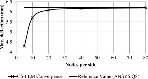
Figure 4: CS-FEM mesh convergence curve

3.2 Preliminary layup optimization of three blade shapes

The developed GA coupled FE solver can be used to optimize the Wageningen-B Series propeller blades against various flow conditions at various speeds. The proposed idea is to extract pressure distribution maps at various speeds above and below the operating (cruise) advance ratio and use the pressure maps as the basis of optimization. Method by which pressure maps are evaluated is at the discretion of the hydrodynamist. These pressure maps have to be used in the optimization scheme’s finite element routine as pressure differences $\left(\Delta P_{ij}\right)$ at each Gauss point calculated with respect to the pressure map at cruise condition. However, this paper focuses on presenting the optimization methodology rather than actual values; thus, pressure values are directly used as the basis for optimization. Pressure variations used in this paper were chosen as uniform arbitrary distributions with no obvious relationship in order to maintain the generality. They were chosen sensibly based on the pressure distribution at cruise condition obtained using CFD (ANSYS CFX) analyzes in preliminary studies (Table 2).

The blades were chosen from the Wageningen-B five bladed series having expanded area ratios (EAR) of 0.75, 0.6 and 0.45. The propellers were chosen to have a diameter of 0.4 m with the hub (boss) having a diameter of 0.08 m respecting the standards of Wageningen-B series. One special characteristic of the Wageningen-B series is all propellers, apart from 4-bladed propellers, have constant pitch distributions in the radial direction [34], making the blades 2-dimensional on the plane of the blade. Thus, 2-dimensional meshes were generated for these three blade shapes using 3-noded triangular elements (Figure 5). The chosen pressure distributions and required pitch to diameter ratios are given in Table 2. Further note that unlike a Controllable Pitch Propeller (CPP), a passive shape adaptive propeller cannot change its pitch at the hub. Thus, the pitch values presented in Table 2 and throughout this paper are pitch values required at the tip of the blade.

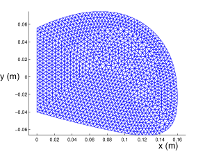
(a)

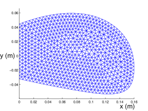
(b)

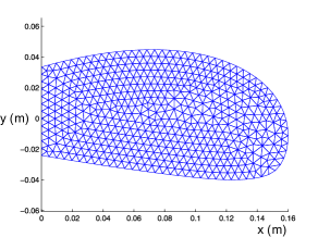
(c)

Figure 5: T3 meshes generated for blade shapes; (a) B5-75, (b) B5-60, (c) B5-45

P (kPa)	$\Delta$P (kPa)	P/D	$\phi$ (deg)	$\Delta\phi$ (deg)
180	-70	0.7	12.56	-3.44
205	-45	0.8	14.3	-1.7
250 (Cruise)	0	0.9	16	0
270	+20	1.0	17.66	+1.66
300	+50	1.1	19.3	+3.3

Table 2: Pressure variations and required optimum pitch values

The optimization was carried out using prepreg AS4 carbon fiber reinforced 3501-6 epoxy with a nominal layer thickness of 125 μm (Table 3 [35]). It was considered that the blades were made of 40 layers. The lay up was taken to be symmetric (i.e. - $\left[B\right]=\left[0\right]$) to prevent warping during the manufacturing process. Thus, the optimization algorithm was used to optimize 20 independent variables. It was initially assumed that any fiber angle is possible to be manufactured; thus, optimization was performed assuming ply angles could be any real number (continuous variable ply optimization). Integer ply optimization was also attempted and will be demonstrated in the proceeding section. Ply angle results obtained using the optimization process, required to enable the optimum pitch variation is given in Table 4 (all ply angle results specified in this paper are measured counter-clockwise from x-axis to y-axis with coordinate system specified in Figure 5).

Property	Value
E1(GPa)	126
E2 (GPa)	11
G12 (GPa)	6.6
ν12	0.28
ν23	0.4
Thickness (μm)	125

Table 3: AS4-3501-6 Material Properties [35]

Blade	Ply angle configuration (deg)
B5-75	[43.4/10.7/40.1/43.2/15.1/22.9/23.0/30.3/42.7/21.7/11.2/12.7/21.1/11.3/13.7/47.3/21.3/38.2/25.3/41.8]s
B5-60	[40.1/56.2/53.6/14.7/55.1/51.0/46.4/27.7/33.9/32.7/39.1/4.0/52.3/4.0/15.5/123.5/56.1/12.6/9.8/21.9]s
B5-45	[11.7/53.6/28.9/51.6/37.8/28.2/36.6/51.0/51.4/31.0/24.7/13.9/21.8/3.6/35.2/52.0/26.5/26.9/44.2/39.4]s

Table 4: Ply angle results

For the above three blade shapes the genetic algorithm converged to a minimum objective function value of 0.51 deg ($8.86\times 10^{-3}$rad). Figure 6 demonstrates the typical convergence of GA for one of the optimization tasks. The minimum objective function value can be thought of as the average deviation between the required and the achieved result for each pitch angle. Thus, the results were of high satisfaction. Although the requirement of tip angle vs pressure variation was non-linear, the best a passive pitch adapting blade can achieve is a linear tip angle variation with uniform pressure as evident from Figure 7.

Above ply angle results were verified using a commercial FE software (ANSYS) and were found to provide bend-twist coupling characteristics exactly as predicted by the in-house GA coupled FEM code. Thus, the coupled code for GA and FEM can be used to optimize ply angles based on the required deformation. Figure 7 demonstrates the comparison between achieved pitch angle and required pitch angle. All three blade shapes behaved similarly and were able to achieve the same pitch angles; thus, for brevity, only one comparison is presented in Figure 7.

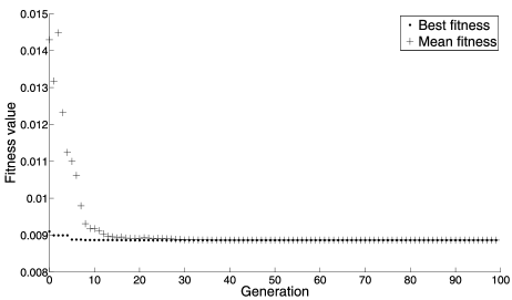
Figure 6: Typical Convergence of the Genetic Algorithm

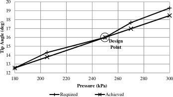
Figure 7: Comparison between pitch angles

3.3 Further analysis of Wageningen B5-45

The Wageningen B5-45 blade was further analyzed for a weighted off-design point case, integer optimization and the effect of layer thickness. The unloaded shape required to behave according to Table 2 was also obtained. For the weighted off-design point, it was assumed that the $P=270\,kPa$ point has a relative weightage of 4, while all other off-design points have a relative weightage of 1 (refer to eq. 3). The value of 4 was chosen in this paper purely for demonstration purposes; actual values of weightages have to be evaluated for a particular propeller application based on its probability to operate at each off-design point. Similar to previous cases, continuous ply optimization was performed. Table 5 summarizes the obtained ply angle results and Figure 8 demonstrates and compares the pitch angle variation with equally weighted optimization. Figure 8 demonstrates that assigning weightages enables the achieved pitch curve to move towards more critical off-design point at the expense of deviating further from other off-design points. This is further elaborated by the reduction of difference between the achieved and required tip angle for $270\,kPa$ pressure (Figure 9). Thus, weightages have to be carefully chosen based on the operating conditions of the propeller.

B5-45 (Weighted)

[51.7/58.5/40.9/57.8/55.8/38.5/45.1/40.6/28.8/76.1/32.2/20.3/54.8/58.3/56.1/32.9/63.0/57.9/32.8/106.4]s

(a)

Pressure (kPa)	180	205	250	270	300
Required $\phi$ (deg)	12.56	14.3	16	17.66	19.3
Non-weighted $\phi$ (deg)	12.56	13.79	16	16.98	18.46
Weighted $\left(w_{4}=4\right)$$\phi$ (deg)	11.38	13.03	16	17.32	19.3

(b)

Table 5: Weighted ply angle results; (a) Ply angles (degrees), (b) Resulting pitch angles

Figure 8: Tip angle results for weighted optimization case

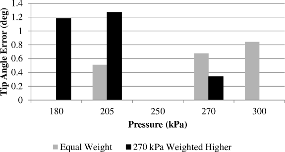
Figure 9: Difference between achieved and required tip angles for non-weighted and weighted cases

Integer ply optimization was performed for equal weighting case. Integer ply optimization is preferable as it greatly simplifies the lay up and manufacturing process. It was observed that integer ply optimization problems required a considerably longer time to converge at a result compared to continuous ply optimization problems. Integer ply optimization was performed for four cases: only integer ply angles $\left(0\leq\theta<\pi\right)$ are allowed, only products of 5 degrees are allowed, only products of 10 degrees are allowed and only angles $\left\{0\text{\textdegree},30\text{\textdegree},45\text{\textdegree},60\text{\textdegree},90\text{\textdegree},120\text{\textdegree},135\text{\textdegree},150\text{\textdegree}\right\}$ are allowed. Results of these optimization problems are given in Table 6. It was observed that for the first three cases, the objective function was able to achieve the same minimum value obtained for continuous ply optimization. Thus, limiting the variable domain was not detrimental towards final results. The last case with more aggressive variable domain limitations was found to increase the value of the objective function. Hence, the achieved tip angles further deviated from the required tip angles.

Case	Ply Angle Result (deg)	$f_{min}\>(rad)$
All Integer	[92/66/107/45/34/31/59/27/71/35/38/34/68/89/108/22/5/79/119/29]s	$8.86\times 10^{-3}$
Only 5n deg	[75/55/75/40/35/45/50/90/25/15/80/100/130/30/90/80/65/55/65/90]s	$8.86\times 10^{-3}$
Only 10n deg	[30/90/90/60/40/40/50/40/20/30/40/10/80/160/30/40/70/120/30/90]s	$8.86\times 10^{-3}$
Limited Ply Angles	[(60)9/90/60/90/150/60/135/(150)5]s	$4.41\times 10^{-2}$

Table 6: Integer ply optimization results

All above optimization tasks were carried out as unconstrained optimization. One of the major drawbacks witnessed was the high flexibility of the resulting blade, which resulted in a substantial rake deformation in the process of pitch variation. It was investigated whether the flexibility can be reduced by increasing the number of layers on the blade. Inasmuch as, an attempt was made to optimize the blade assuming there are 50 CFRP prepreg layers all having a nominal thickness of $125\mu m$ (Table 3). It was observed that, increasing the number of layers resulted in a stiffer blade, which had relatively less bend-twist coupling performance compared to the 40 layer blades attempted earlier (Table 7). However, the same twisting performance was able to be achieved if the total laminate thickness of the 50 layer layup was the same as the 40 layer layup; in other words, if the nominal layer thickness of CFRP layers were reduced to $100\mu m.$ The resulting blade had the same twisting performance as the 40 layer model, but with a less lateral deformation. This was enabled by its higher bend-twist coupling coefficient in the bending compliance matrix ($\left[d\right]$). In addition, the layup with 40 $100\mu m$ layers had the same twisting performance with a higher lateral bend. It must be noted that, layer thickness is a practical limitation under the current composite prepreg lamina manufacturing technology that is beyond composite designer’s control. However, it was clear that in order achieve best bend-twist coupling performance one must attempt to reduce the the layer thickness while increasing the number of layers in the laminate. Table 7 summarizes results obtained for different layer numbers.

Layers	Layer Thk. ($\mu m$)	Total Thk. (mm)	Optimum Layup (deg)	$f_{min}\>(rad)$
40	125	5	[11.7/53.6/28.9/51.6/37.8/28.2/36.6/51.0/51.4/31.0/24.7/	0.00886
			13.9/21.8/3.6/35.2/52.0/26.5/26.9/44.2/39.4]s
50	125	6.25	[41.9/41.9/78.8/41.6/43.5/42.3/45.1/79.4/42.8/41.6/78.8/44.8/44.4/	0.0134
			41.5/44.1/41.5/79.2/45.1/79.0/41.0/80.4/43.0/45.7/41.7/81.2]s
50	100	5	[32.1/46.4/44.8/55.6/50.3/52.5/43.2/2.1/22.4/50.2/21.1/17.2/36.6/	0.00886
			36.5/13.5/40.8/38.1/49.3/45.3/26.9/52.3/12.2/55.8/8.8/3.3]s
40	100	4	[4.1/30.3/11.3/7.6/24.3/109.4/60.4/0.41/42.9/15.7/15.2/	0.00886
			49.6/39.1/33.2/110.7/113.9/83.7/46.7/64.4/97.5]s
20	250	5	[15.7/19.7/30.3/49.7/37.2/44.3/22.1/34.9/47.0/3.4]s	0.00886

Table 7: Results for different layer thicknesses

Note further that the current unconstrained optimization scheme is capable of satisfying the pitch angle variation requirement almost perfectly greatly enhancing the efficiency envelope. However, this may not be possible due to the considerable increase in flexibility and lateral deformations. Optimization constraints must be introduced based on the application to limit such deformations at the expense of efficiency gains.

3.4 Unloaded shape calculation

The second stage of the proposed design process is the calculation of the unloaded blade shape. The process is iteration based where negative loads are applied to the shape at the design/cruise speed of blade. Once the first unloaded shape is obtained, the loads at design speed are applied to the unloaded shape to check whether it reaches the desired shape at the operating speed. The desired shape is the shape of the optimum alloy propeller chosen. If the shape requirement has not been met, the initial shape is adjusted by the difference and further iterated until there is satisfactory shape convergence (Figure 10).

Figure 10: Unloaded shape iteration process

The unloaded shape for the B5-45 blade was calculated for the layup given in Table 4. As summarized in Figure 10, the first step of the process was to apply reverse strains or reverse loads. In this example reverse loads were applied. If reverse strains were applied the iteration path would be different, but will eventually converge to the same unloaded shape. Based on the iterations it was concluded that the blade has to be manufactured with an initial uniform twist of 16^o pitch angle at the root and 4.53^o at the tip. Further loading due to the movement of the ship is expected to increase the pitch of the propeller. Summary of iteration values is presented in Table 8. These values are depicted in Figure 11 for better representation.

Iteration	Ini. Tip	Loaded Tip	%Error	Adjustment
1	3.44o	14.76o	7.73	1.24o
2	4.68o	16.18o	-1.11	-0.18o
3	4.50o	15.97o	0.17	-0.03o
4	4.53o	16.00o	-0.03	0.00o

Table 8: Unloaded shape iteration steps

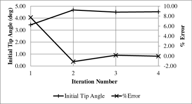
Figure 11: Unloaded shape iteration summary

4 Conclusion

The paper presented an optimization scheme for optimizing the ply lay up of composite marine propeller blades using a coupled Genetic Algorithm and Finite Element approach. The genetic algorithm was utilized to vary the ply angles based on their fitness values while the Cell-Based Smoothed FE code using Discrete Shear Gap Method, was used to evaluate the deflection and pitch of the blade under given loadings. Pressure distributions were chosen to be uniform and arbitrary, letting the readers to use exact pressure distribution functions using CFD methods. Continuous ply optimization was performed for three blade shapes to demonstrates the design scheme applicability for various shapes. Further, B5-45 was analyzed for weighted off-design point optimization, integer ply optimization and effect of different layer thicknesses. Unloaded shape for B5-45 was also calculated and was found to provide good convergence. Results obtained using the coupled optimization algorithm had a high accuracy and the process can be confidently used in future research endeavors. The framework presented in the paper was purely based on optimization for best efficiency using shape adaptability achieved through optimization of composite layup angles. There are many steps and adjustments to be made based on strength testing, cavitation performance testing, natural frequency and structural divergence analysis, etc. Thus, the proposed framework can be seen as a foundation for designing shape-adaptive composite marine propellers.

References

References

- [1] Y.-J. Lee, C.-C. Lin, Optimized design of composite propeller, Mech. Adv. Mater. Struc. 11 (1) (2004) 17–30.
- [2] Y. L. Young, Hydroelastic behavior of flexible composite propellers in wake inflow, in: 16th International Conference on Composite Materials, Kyoto, Japan, 2007.
- [3] Z. Liu, Y. L. Young, Utilization of bendtwist coupling for performance enhancement of composite marine propellers, J. Fluid. Struct. 25 (6) (2009) 1102–1116.
- [4] N. L. Mulcahy, B. G. Prusty, C. Gardiner, Hydroelastic design of composite components, Int. J. Ship Offshore Struct. 5 (4) (2010) 359–370.
- [5] M. R. Motley, Y. L. Young, Performance-based design and analysis of flexible composite propulsors, J. Fluid Struct. 27 (8) (2011) 1310–1325.
- [6] N. L. Mulcahy, B. G. Prusty, C. P. Gardiner, Flexible composite hydrofoils and propeller blades, T. Roy. I. Nav. Archit. B - Int. J. Small Craft Technol. 153 (1) (2011) B39–B46.
- [7] C. C. Lin, Y. J. Lee, C. S. Hung, Optimization and experiment of composite marine propellers, Compos. Struct. 89 (2) (2009) 206–215.
- [8] C.-C. Lin, Y.-J. Lee, Stacking sequence optimization of laminated composite structures using genetic algorithm with local improvement, Compos. Struct. 63 (34) (2004) 339–345.
- [9] M. M. Plucinski, Y. L. Young, Z. Liu, Optimization of a self-twisting composite marine propeller using genetic algorithms, in: 16th International Conference on Composite Materials, Kyoto, Japan, 2007.
- [10] A. Noor, W. Burton, Assessment of shear deformation theories for multilayered composite plates, ASME Appl. Mech. Rev. 42 (1989) 1–13.
- [11] Mallikarjuna, T. Kant, A critical review and some results of recently developed refined theories of fibre reinforced laminated composites and sandwiches, Compos. Struct. 23 (1993) 293–312.
- [12] T. Kant, K. Swaminathan, Estimation of transverse/interlaminar stresses in laminated composites - a selective review and survey of current developments, Compos. Struct. 49 (2000) 65–75.
- [13] R. Khandan, S. Noroozi, P. Sewell, J. Vinney, The development of laminated composite plate theories: a review, J. Mater. Sci. 47 (2012) 5901–5910.
- [14] G. Liu, K. Dai, T. Nguyen, A smoothed finite elemen for mechanics problems, Comput. Mech. 39 (2007) 859–877.
- [15] H. Nguyen-Xuan, S. Bordas, H. Nguyen-Dang, Smooth finite element methods: convergence, accuracy and properties, Int. J. Numer. Meth. Eng. 74 (2008) 175–208.
- [16] S. Bordas, S. Natarajan, On the approximation in the smoothed finite element method (SFEM), Int. J. Numer. Meth. Eng. 81 (2010) 660–670.
- [17] G. Liu, T. Nguyen-Thoi, H. Nguyen-Xuan, K. Lam, A node based smoothed finite element (NS-FEM) for upper bound solution to solid mechanics problems, Comput. Struct. 87 (2009) 14–26.
- [18] G. Liu, T. Nguyen-Thoi, K. Lam, An edge-based smoothed finite element method (ES-FEM) for static, free and forced vibration analyses of solids, J. Sound Vib. 320 (2009) 1100–1130.
- [19] T. Nguyen-Thoi, G. Liu, K. Lam, G. Zhang, A face-based smoothed finite element method (FS-FEM) for 3D linear and nonlinear solid mechanics using 4-node tetrahedral elements, Int. J. Numer. Meth. Eng. 78 (2009) 324–353.
- [20] G. Liu, T. Nguyen-Thoi, K. Lam, A novel alpha finite element method (fem) for exact solution to mechanics problems using triangular and tetrahedral elements, Comput. Method. Appl. M. 197 (2008) 3883–3897.
- [21] F. Cazes, G. Meschke, An edge based imbricate finite element method (ei-fem) with full and reduced integration, Comput. Struct. 106-107 (2012) 154–175.
- [22] N. T. Nguyen, T. Rabczuk, H. Nguyen-Xuan, S. Bordas, A smoothed finite element method for shell analysis, Comput. Method. Appl. M. 198 (2008) 165–177.
- [23] S. Wu, G. Liu, X. Cui, T. Ngyuen, G. Zhang, An edge-based smoothed point interpolation method ES-PIM for heat transfer analysis of rapid manufacturing system, Int. J. Heat Mass Transfer 53 (2010) 1938–1950.
- [24] H. Nguyen-Xuan, G. Liu, S. Bordas, S. Natarajan, T. Rabczuk, Ad adaptive singular ES-FEM for mechanics problems with singular field of arbitrary order, Comput. Method. Appl. M. 253 (2013) 252–273.
- [25] Z. He, A. Cheng, G. Zhang, Z. Zhong, G. Liu, Dispersion error reduction for acoustic problems using the edge based smoothed finite element method (ES-FEM), Int. J. Numer. Meth. Eng. 86 (2011) 1322–1338.
- [26] S. Bordas, S. Natarajan, P. Kerfriden, C. Augarde, D. R. Mahapatra, T. Rabczuk, S. D. Pont, On the performance of strain smoothing for quadratic and enriched finite element approximation (XFEM/GFEM/PUFEM), Int. J. Numer. Meth. Eng. 86 (2011) 637–666.
- [27] Y. J. Lee, C. C. Lin, J. C. Ji, J. S. Chen, Optimization of a composite rotor blade using a genetic algorithm with local search, J. Reinf. Plast. Compos. 24 (16) (2005) 1759–1769.
- [28] M. T. Herath, B. G. Prusty, Performance analysis and optimization of bend-twist coupled composite hydrofoils using fluid-structure interaction, in: 7th Australasian Congress on Applied Mechanics, Adelaide, Australia, 2012.
- [29] M. T. Herath, S. Natarajan, B. G. Prusty, N. St John, Shape-adaptive composite marine propellers: Analysis and optimization, in: 19th International Conference on Composite Materials, Montreal, Canada, 2013.
- [30] M. Kameyama, H. Fukunaga, Optimum design of composite plate wings for aeroelastic characteristics using lamination parameters, Comput. Struct. 85 (34) (2007) 213–224.
- [31] G. Soremekun, Z. Gurdal, R. T. Haftka, L. T. Watson, Composite laminate design optimization by genetic algorithm with generalized elitist selection, Comput. Struct. 79 (2) (2001) 131–143.
- [32] T. Nguyen-Thoi, P. Phung-Van, H. Nguyen-Xuan, C. Thai-Hoang, A cell-based smoothed discrete shear gap method using triangular elements for static and free vibration analyses of Reissner-Mindlin plate, International Journal for Numerical Methods in Engineering (2012) 705–741], volume=91.
- [33] K. U. Bletzinger, M. Bischoff, E. Ramm, A unified approach for shear-locking free triangular and rectangular shell finite elements, Int. J. Numer. Meth. Eng. 75 (2000) 321–334.
- [34] G. Kuiper, The Wageningen Propeller Series, Maritime Research Institute Netherlands, The Netherlands, 1992.
- [35] P. D. Soden, M. J. Hinton, A. S. Kaddour, Lamina properties, lay-up configurations and loading conditions for a range of fibre-reinforced composite laminates, Compos. Sci. Technol. 58 (7) (1998) 1011–1022.