Computable estimates of the distance to the exact solution of the evolutionary reaction-diffusion equation

Abstract

We derive guaranteed bounds of distance to the exact solution of the evolutionary reaction-diffusion problem with mixed Dirichlet–Neumann boundary condition. It is shown that two-sided error estimates are directly computable and equivalent to the error. Numerical experiments confirm that estimates provide accurate two-sided bounds of the overall error and generate efficient indicators of local error distribution.

1 Problem statement

Let $\Omega\in{\mathds{R}}^{d}$ ($d=$ 1, 2, or 3) be a bounded connected domain with Lipchitz continuous boundary $\partial\Omega$, which consists of two measurable non-intersecting parts $\Gamma_{D}$ and $\Gamma_{N}$ associated with Dirichlet and Neumann boundary conditions, respectively. Let $Q_{T}$ denote the space-time cylinder $Q_{T}:=\Omega\times(0,T)$, $T>0$. The lateral surface of $Q_{T}$ is denoted by $S_{T}:=\partial\Omega\times[0,T]=\big{(}\Gamma_{D}\cup\Gamma_{N}\big{)}\times[0,T]=S_{D}\cup S_{N}$.

We consider the classical reaction-diffusion initial boundary value problem

$$u_{t}-\nabla\cdot p+\lambda u =\,f, \quad(x,t)\in Q_{T},$$ (1)

$$p =\,A\nabla u, \quad(x,t)\in Q_{T},$$

$$u(x,0) =\,\varphi, \quad x\in\Omega,$$ (2)

$$u =\,0, \quad(x,t)\in S_{D},$$ (3)

$$p\cdot n =\,g, \quad(x,t)\in S_{N},$$ (4)

where $n$ denotes the vector of unit outward normal to $\partial\Omega$, and

$$f(x,t)\in L^{2}(Q_{T}),\quad\varphi(x)\in L^{2}(\Omega),\quad{g(x,t)\in L^{2}\left(0,T;L^{2}(\Gamma_{N})\right).}$$ (5)

The function $\lambda$ entering the reaction part of (1) is non-negative bounded function, and its values may drastically vary on different parts of the domain. Also, we assume that for a.e. $t\in(0,T)$ the matrix $A$ is symmetric and satisfies the condition

$$\nu_{1}|\xi|^{2}\leq A(x)\>\xi\cdot\xi\leq\nu_{2}|\xi|^{2},\quad\xi\in{\mathds{R}}^{d},\quad 0<\nu_{1}\leq\nu_{2}<\infty,\quad\mbox{for a.e.}\quad x\in\Omega.$$ (6)

Henceforth, we use the following notation

$$\|\>\tau\>\|^{2}_{A}=\int\limits_{\Omega}A\tau\cdot\tau\mathrm{\>d}x,\quad\|\>\tau\>\|^{2}_{A^{-1}}=\int\limits_{\Omega}A^{-1}\tau\cdot\tau\mathrm{\>d}x,\quad{\mid\!\mid\!\mid\!\tau\!\mid\!\mid\!\mid}^{2}=\int\limits_{Q_{T}}A\tau\cdot\tau\mathrm{\>d}x\mathrm{d}t,\quad{\mid\!\mid\!\mid\!\tau\!\mid\!\mid\!\mid}^{2}_{*}=\int\limits_{Q_{T}}A^{-1}\tau\cdot\tau\mathrm{\>d}x\mathrm{d}t.$$ (7)

By $\|\cdot\|_{\Omega}$ and $\|\cdot\|_{Q_{T}}$ we denote the norms in $L^{2}(\Omega)$ and $L^{2}(Q_{T})$, respectively. The space of functions $g(x,t)$ with the norm $\int\limits_{0}^{T}\|g(\cdot,t)\|_{\Omega}\mathrm{\>d}t$ is denoted by $L^{2,1}(Q_{T})$. ${\mathring{H}}^{1}(Q_{T})$ is a subspace of $H^{1}(Q_{T})$, which contains the functions satisfying (3), ${\mathring{H}}^{1,0}(Q_{T}):=L^{2}\Big{(}(0,T);{\mathring{H}}^{1}(\Omega)\Big{)}$, and $V_{2}(Q_{T}):={\mathring{H}}^{1,0}(Q_{T})\cap L^{\infty}\Big{(}(0,T);L^{2}(\Omega)\Big{)}$. The space $V^{1,0}_{2}(Q_{T}):={\mathring{H}}^{1,0}(Q_{T})\cap C\Big{(}[0,T];L^{2}(\Omega)\Big{)}$ is a subspace of $V_{2}(Q_{T})$ and contains the functions with traces from $L^{2}(\Omega)$ for all $t\in[0,T]$, which continuously changing with $t\in[0,T]$ in the $L^{2}(\Omega)$ norm.

The generalized statement of (1)–(4) is as follows: find a function $u(x,t)\in V^{1,0}_{2}(Q_{T})$ satisfying the integral identity

$$\int\limits_{\Omega}\Big{(}u(x,T)\eta(x,T)-u(x,0)\eta(x,0)\Big{)}\mathrm{\>d}x-\int\limits_{Q_{T}}u\eta_{t}\mathrm{\>d}x\mathrm{d}t+\int\limits_{Q_{T}}A\nabla{u}\cdot\nabla{\eta}\mathrm{\>d}x\mathrm{d}t+\int\limits_{Q_{T}}\lambda u\eta\mathrm{\>d}x\mathrm{d}t=\\ \int\limits_{Q_{T}}f\eta\mathrm{\>d}x\mathrm{d}t+\int\limits_{S_{N}}g\eta\mathrm{\>d}s\mathrm{d}t,\quad\forall\eta\in{\mathring{H}}^{1}(Q_{T}).$$ (8)

Well-known classical solvability results (see, e.g., [6, 7, 3]) guarantee that (1)–(4) has a unique solution in $V^{1,0}_{2}(Q_{T})$ provided that the conditions (5) hold.

Assume that $v\in{\mathring{H}}^{1}(Q_{T})$ presents a certain numerical approximation of $u$. Our goal is to deduce accurate and explicitly computable estimates of the distance between $u$ and $v$. For this purpose, we use the norm

$$[u-v]^{2}_{(\nu,\,\theta,\,\zeta)}:={\mid\!\mid\!\mid\!\nu\,\nabla(u-v)\,\!\mid\!\mid\!\mid}^{2}\>+\>\|\,\theta\,(u-v)\,\|^{2}_{Q_{T}}+\>\|\,\zeta\,(u-v)(x,T)\,\|^{2}_{\Omega},$$ (9)

where $\nu,\theta$, and $\zeta$ are certain positive weights (weight-functions), which balance three components of the error. They can be selected in different ways so that (9) presents a common form of a wide spectrum of different measures.

A fully computable and guaranteed upper bound of $[u-v]^{2}_{(\nu,\,\theta,\,\zeta)}$ is derived in Theorem 1 with the help of the method originally introduced in [15]. In [17], the method was applied to problems with convection, and in [12] the guaranteed error majorants were derived for the Stokes problem. In Section 2, we combine this method with the technique suggested in [14] for the stationary reaction-diffusion problem, which makes it possible to obtain the efficient error majorants for problems with drastically different values of the reaction function. Theorem 1 presents such an estimate for the problem (1)–(4). In Section 3, we derive a guaranteed and fully computable lower bound of the error (9) (Theorem 2). Sections 4 and 5 are devoted to practical applications of the estimates. In them, we discuss numerical results obtained for several typical examples, which confirm the efficiency of two-sided bounds.

2 Error majorant

Let $e(x,t):=(u-v)(x,t)$ denote the deviation of $v\in{\mathring{H}}^{1}(Q_{T})$ from the exact solution $u$. From (8), it follows that

$$\int\limits_{\Omega}\big{(}e(x,T)\eta(x,T)-e(x,0)\eta(x,0)\big{)}\mathrm{\>d}x-\int\limits_{Q_{T}}e\eta_{t}\mathrm{\>d}x\mathrm{d}t+\int\limits_{Q_{T}}A\nabla{e}\cdot\nabla{\eta}\mathrm{\>d}x\mathrm{d}t+\int\limits_{Q_{T}}\lambda e\eta\mathrm{\>d}x\mathrm{d}t=\\ \int\limits_{Q_{T}}\left(f-v_{t}-\lambda v\right)\eta\mathrm{\>d}x\mathrm{d}t-\int\limits_{Q_{T}}A\nabla{v}\cdot\nabla{\eta}\mathrm{\>d}x\mathrm{d}t+\int\limits_{S_{N}}g\eta\mathrm{\>d}s\mathrm{d}t.$$ (10)

Since $e\in{\mathring{H}}^{1}(Q_{T})$, we can set $\eta=e$ and, using the relation

$$\int\limits_{\Omega}\left(e^{2}(x,T)-e^{2}(x,0)\right)\mathrm{\>d}x-\int\limits_{Q_{T}}ee_{t}\mathrm{\>d}x\mathrm{d}t=\frac{1}{2}\left(\|\,e(x,T)\,\|^{2}_{\Omega}-\|\,e(x,0)\,\|^{2}_{\Omega}\right),$$ (11)

obtain

$$\frac{1}{2}\|\,e(x,T)\,\|^{2}_{\Omega}+{\mid\!\mid\!\mid\!\nabla{e}\!\mid\!\mid\!\mid}^{2}+\left\|\sqrt{\lambda}e\,\right\|^{2}_{Q_{T}}=\\ \int\limits_{Q_{T}}\left(f-v_{t}-\lambda v\right)e\mathrm{\>d}x\mathrm{d}t-\int\limits_{Q_{T}}A\nabla{v}\cdot\nabla e\mathrm{\>d}x\mathrm{d}t+\int\limits_{S_{N}}ge\mathrm{\>d}s\mathrm{d}t+\frac{1}{2}\|\,e(x,0)\,\|^{2}_{\Omega}\,.$$ (12)

This relation is a form of the ‘energy-balance’ identity in terms of deviation. It plays an important role in subsequent analysis. Now, we introduce an additional variable $y\in Y_{\mathrm{div}\>}(Q_{T})$, where

$$Y_{\mathrm{div}\>}(Q_{T}):=\left\{\>y(x,t)\in L^{2}(\Omega,{\mathds{R}}^{d})\;\;\big{|}\;\;\mathrm{div}\>y(x,t)\in L^{2}(\Omega),\;\;y\cdot n\in L^{2}(\Gamma_{N})\;\;{\mbox{for a.e.}}\;\;t\in(0,T)\>\right\}.$$ (13)

Theorem 1

(i) For any $v\in{\mathring{H}}^{1}(Q_{T})$ and $y\in Y_{\mathrm{div}\>}(Q_{T})$ the following inequality holds

$$(2-\delta){\mid\!\mid\!\mid\!\nabla e\!\mid\!\mid\!\mid}^{2}+\left(2-\frac{1}{\gamma}\right)\left\|\sqrt{\lambda}e\,\right\|^{2}_{Q_{T}}+\|\,e(x,T)\,\|^{2}_{\Omega}=:{[e]\,}^{2}_{(\overline{\nu},\,\overline{\theta},\,\overline{\zeta})}\leq\overline{\mathrm{M}}^{2}_{(\delta,\,\gamma,\,\mu)}(v,y):=\\ \|\,e(0,x)\,\|^{2}_{\Omega}+\int\limits_{0}^{T}\Bigg{(}\gamma\bigg{\|}\,\frac{\mu}{\sqrt{\lambda}}\,\mathscr{R}_{f}(v,y)\,\bigg{\|}^{2}_{\Omega}\>+\alpha_{1}(t)\frac{C_{\mathrm{F\Omega}}^{2}}{\nu_{1}}\|\,(1-\mu)\,\mathscr{R}_{f}(v,y)\,\|^{2}_{\Omega}\>+\\ \alpha_{2}(t)\|\,\mathscr{R}_{d}(v,y)\,\|^{2}_{A^{-1}}+\alpha_{3}(t)\frac{C_{\mathrm{tr}}^{2}}{\nu_{1}}\big{\|}\,\mathscr{R}_{b}(v,y)\,\big{\|}^{2}_{\Gamma_{N}}\Bigg{)}\mathrm{\>d}t,$$ (14)

where

$$\mathscr{R}_{f}(v,y)=f-v_{t}-\lambda v+\mathrm{div}\>y,\quad\mathscr{R}_{d}(v,y)=y-A\nabla{v},\quad\mathscr{R}_{b}(v,y)=g-y\cdot n,$$ (15)

$C_{\mathrm{F\Omega}}$ is the constant from the Friedrichs’ inequality

$$\|\,\bar{\eta}\,\|_{\Omega}\leq C_{\mathrm{F\Omega}}\|\,\nabla\bar{\eta}\,\|_{\Omega},\qquad\forall\bar{\eta}\in{\mathring{H}}^{1}(\Omega),$$ (16)

$C_{\mathrm{tr}}$ is the constant in the trace inequality

$$\|\,\bar{\eta}\,\|_{\Gamma_{N}}\leq C_{\mathrm{tr}}\|\,\nabla\bar{\eta}\,\|_{\Omega},\qquad\forall\bar{\eta}\in{\mathring{H}}^{1}(\Omega).$$ (17)

Here, $\overline{\nu}=\sqrt{2-\delta}$, $\overline{\theta}=\sqrt{2-\frac{1}{\gamma}}$, $\overline{\zeta}=1$ are positive weights, where $\delta\in(0,2]$, $\gamma\in\Big{[}\frac{1}{2},+\infty\Big{[}$; $\mu(x,t)$ is a real-valued function taking values in $[0,1]$; and $\alpha_{1}(t)$, $\alpha_{2}(t)$, $\alpha_{3}(t)$ are positive scalar-valued functions satisfying the relation

$$\frac{1}{\alpha_{1}(t)}+\frac{1}{\alpha_{2}(t)}+\frac{1}{\alpha_{3}(t)}=\delta.$$ (18)

(ii) For any $\delta\in(0,2]$, $\gamma\in\Big{[}\frac{1}{2},+\infty\Big{[}$, and a real-valued function $\mu(x,t)$ taking values in $[0,1]$, the lower bound of the variation problem

$$\inf\limits_{\begin{array}[]{c}v\in{\mathring{H}}^{1}(Q_{T})\\ y\in Y_{\mathrm{div}\>}(Q_{T})\end{array}}\overline{\mathrm{M}}^{2}_{(\delta,\,\gamma,\,\mu)}(v,y)$$ (19)

is zero, and it is attained if and only if $v=u$ and $y=A\nabla u$.

Proof. (i) We transform the right-hand side of (12) by means of the relation

$$\int\limits_{Q_{T}}\mathrm{div}\>y\,e\mathrm{\>d}x\mathrm{d}t+\int\limits_{Q_{T}}y\cdot\nabla{e}\mathrm{\>d}x\mathrm{d}t=\int\limits_{S_{N}}y\cdot n\,e\mathrm{\>d}s\mathrm{d}t,$$ (20)

which yields

$$\frac{1}{2}\|\,e(x,T)\,\|^{2}_{\Omega}+{\mid\!\mid\!\mid\!\nabla{e}\!\mid\!\mid\!\mid}^{2}+\left\|\sqrt{\lambda}e\,\right\|^{2}_{Q_{T}}=\mathscr{I}_{f}+\mathscr{I}_{d}+\mathscr{I}_{b}+\frac{1}{2}\|\,e(x,0)\,\|^{2}_{\Omega},$$ (21)

where

$$\mathscr{I}_{f}=\int\limits_{Q_{T}}\mathscr{R}_{f}(v,y)\,e\mathrm{\>d}x\mathrm{d}t,\quad\mathscr{I}_{d}=\int\limits_{Q_{T}}\mathscr{R}_{d}(v,y)\cdot\nabla{e}\mathrm{\>d}x\mathrm{d}t,\quad\mathscr{I}_{b}=\int\limits_{S_{N}}\mathscr{R}_{b}(v,y)\,e\mathrm{\>d}s\mathrm{d}t.$$ (22)

By means of the Hölder’s inequality, we find that

$$\mathscr{I}_{d}=\int\limits_{Q_{T}}\mathscr{R}_{d}(v,y)\cdot\nabla{e}\mathrm{\>d}x\mathrm{d}t\leq\int\limits_{0}^{T}\left\|\,\mathscr{R}_{d}(v,y)\,\right\|_{A^{-1}}\|\,\nabla{e}\,\|_{A}\mathrm{\>d}t$$ (23)

and

$$\mathscr{I}_{b}=\int\limits_{S_{N}}\mathscr{R}_{b}(v,y)\,e\mathrm{\>d}s\mathrm{d}t\leq\int\limits_{0}^{T}\left\|\,\mathscr{R}_{b}(v,y)\,\right\|_{\Gamma_{N}}\|\,e\,\|_{\Gamma_{N}}\mathrm{\>d}t\leq\int\limits_{0}^{T}\left\|\,\mathscr{R}_{b}(v,y)\,\right\|_{\Gamma_{N}}\frac{C_{\mathrm{tr}}}{\sqrt{\nu_{1}}}\|\,\nabla{e}\,\|_{A}\mathrm{\>d}t,$$ (24)

where $\nu_{1}$ appears due to (6). Let $\mu(x,t)$ be a real-valued function taking values in $[0,1]$. Then, we estimate the term $\mathscr{I}_{f}$ as follows:

$$\mathscr{I}_{f}\leq\bigintsss\limits_{0}^{T}\left(\bigg{\|}\,\frac{\mu}{\sqrt{\lambda}}\mathscr{R}_{f}(v,y)\,\bigg{\|}_{\Omega}\left\|\sqrt{\lambda}e\,\right\|_{\Omega}+\frac{C_{\mathrm{F\Omega}}}{\sqrt{\nu_{1}}}\left\|\,(1-\mu)\,\mathscr{R}_{f}(v,y)\,\right\|_{\Omega}\|\,\nabla e\,\|_{A}\right)\mathrm{\>d}t.$$ (25)

In [14], this decomposition was used in order to overcome difficulties arising in the stationary problem if $\lambda$ is small (or close to zero) in some parts of the domain (a more detailed study of this form of the majorant can be found in [11, 9]).

Combining (23), (23), and (25), we obtain

$$\frac{1}{2}\|\,e(x,T)\,\|^{2}_{\Omega}+{\mid\!\mid\!\mid\!\nabla e\!\mid\!\mid\!\mid}^{2}+\left\|\,\sqrt{\lambda}e\,\right\|^{2}_{Q_{T}}\leq\frac{1}{2}\|\,e(x,0)\,\|^{2}_{\Omega}+\int\limits_{0}^{T}\Bigg{(}\bigg{\|}\,\frac{\mu}{\sqrt{\lambda}}\,\mathscr{R}_{f}(v,y)\,\bigg{\|}_{\Omega}\Big{\|}\,\sqrt{\lambda}\,e\Big{\|}_{\Omega}+\\ \frac{C_{\mathrm{F\Omega}}}{\sqrt{\nu_{1}}}\left\|\,(1-\mu)\,\mathscr{R}_{f}(v,y)\,\right\|_{\Omega}\|\,\nabla e\,\|_{A}+\left\|\,\mathscr{R}_{d}(v,y)\,\right\|_{A^{-1}}\|\,\nabla e\,\|_{A}+\left\|\,\mathscr{R}_{b}(v,y)\,\right\|_{\Gamma_{N}}\frac{C_{\mathrm{tr}}}{\sqrt{\nu_{1}}}\|\,\nabla e\,\|_{A}\Bigg{)}\mathrm{\>d}t.$$ (26)

The second term on the right-hand side of (26) can be estimated by the Young–Fenchel inequality

$$\int\limits_{0}^{T}\bigg{\|}\,\frac{\mu}{\sqrt{\lambda}}\,\mathscr{R}_{f}(v,y)\,\bigg{\|}_{\Omega}\left\|\sqrt{\lambda}\,e\,\right\|_{\Omega}\mathrm{\>d}t\leq\int\limits_{0}^{T}\left(\frac{\gamma}{2}\bigg{\|}\,\frac{\mu}{\sqrt{\lambda}}\,\mathscr{R}_{f}(v,y)\,\bigg{\|}^{2}_{\Omega}+\frac{1}{2\gamma}\left\|\,\sqrt{\lambda}e\,\right\|^{2}_{\Omega}\right)\mathrm{\>d}t,$$ (27)

where $\gamma$ is an arbitrary real parameter from $\Big{[}\frac{1}{2},+\infty\Big{[}$. Analogously,

$$\int\limits_{0}^{T}\frac{C_{\mathrm{F\Omega}}}{\sqrt{\nu_{1}}}\left\|\,(1-\mu)\,\mathscr{R}_{f}(v,y)\,\right\|_{\Omega}\|\,\nabla e\,\|_{A}\mathrm{\>d}t \leq\int\limits_{0}^{T}\left(\frac{\alpha_{1}(t)}{2}\frac{C_{\mathrm{F\Omega}}^{2}}{\nu_{1}}\left\|\,(1-\mu)\,\mathscr{R}_{f}(v,y)\,\right\|^{2}_{\Omega}+\frac{1}{2\alpha_{1}(t)}\|\,\nabla e\,\|^{2}_{A}\right)\mathrm{\>d}t,$$ (28)

$$\int\limits_{0}^{T}\|\,\mathscr{R}_{d}(v,y)\,\|_{A^{-1}}\|\,\nabla e\,\|_{A}\mathrm{\>d}t \leq\int\limits_{0}^{T}\left(\frac{\alpha_{2}(t)}{2}\left\|\,\mathscr{R}_{d}(v,y)\,\right\|^{2}_{A^{-1}}+\frac{1}{2\alpha_{2}(t)}\|\,\nabla e\,\|^{2}_{A}\right)\mathrm{\>d}t,$$ (29)

and

$$\int\limits_{0}^{T}\left\|\,\mathscr{R}_{b}(v,y)\,\right\|_{\Gamma_{N}}\frac{C_{\mathrm{tr}}}{\sqrt{\nu_{1}}}\|\,\nabla e\,\|_{A}\mathrm{\>d}t\leq\int\limits_{0}^{T}\left(\frac{\alpha_{3}(t)}{2}\frac{C_{\mathrm{tr}}^{2}}{\nu_{1}}\left\|\,\mathscr{R}_{b}(v,y)\,\right\|^{2}_{\Gamma_{N}}+\frac{1}{2\alpha_{3}(t)}\|\,\nabla e\,\|^{2}_{A}\right)\mathrm{\>d}t.$$ (30)

Here, $\alpha_{1}(t)$, $\alpha_{2}(t)$, and $\alpha_{3}(t)$ are functions satisfying (18). The estimate (14) follows from (27)–(30).

(ii) Existence of the pair $(v,y)\in{\mathring{H}}^{1}(Q_{T})\times Y_{\mathrm{div}\>}(Q_{T})$ minimizing the functional $\overline{\mathrm{M}}^{2}_{(\delta,\,\gamma,\,\mu)}(v,y)$ can be proven straightforwardly. Indeed, let $v=u$ and $y=A\nabla u$. Since $\mathrm{div}\>(A\nabla u)\in L^{2}(Q_{T})$, we see that $y\in Y_{\mathrm{div}\>}(Q_{T})$. In this case, $e(0,x)=(u-v)(0,x)=\varphi(x)-v(0,x)=0$,   $\mathscr{R}_{f}(u,A\nabla u)=f-u_{t}-\lambda u+\mathrm{div}\>A\nabla u=0$,   $\mathscr{R}_{d}(u,A\nabla u)=A\nabla u-A\nabla{u}=0$, and $\mathscr{R}_{b}(v,y)=g-A\nabla u\cdot n=0$. Then, $\overline{\mathrm{M}}^{2}_{(\delta,\,\gamma,\,\mu)}(u,A\nabla u)=0$, and the exact lower bound is attained.

On the other hand, if $\overline{\mathrm{M}}^{2}_{(\delta,\,\gamma,\,\mu)}(v,y)=0$, then $v$ satisfies the initial and boundary conditions, and for a.e. $(x,t)\in Q_{T}$ the following relations hold:

$$y=A\nabla v,\quad f-v_{t}-\lambda v+\mathrm{div}\>y=0.$$ (31)

From (31), it follows that

$$\int\limits_{Q_{T}}(f-v_{t}-\lambda v)\eta\mathrm{\>d}x\mathrm{d}t-\int\limits_{Q_{T}}y\cdot\nabla{\eta}+\int\limits_{S_{N}}g\eta\mathrm{\>d}s\mathrm{d}t=0,\quad\forall\eta\in{\mathring{H}}^{1}(Q_{T}).$$ (32)

The identity (32) is equivalent to (8). Hence, $v=u$, and we see that $\overline{\mathrm{M}}^{2}_{(\delta,\,\gamma,\,\mu)}(v,y)$ vanishes if and only if

$$f-v_{t}-\lambda v+\mathrm{div}\>y =0 \quad{(x,t)}\in Q_{T},$$ a.e.

$$y =A\nabla v \quad{(x,t)}\in Q_{T},$$ a.e.

$$v(x,0) =\varphi(x)\; \quad x\in\Omega,$$ a.e.

$$v =0 \quad{(x,t)}\in S_{D},$$ a.e.

$$y\cdot n =g \quad{(x,t)}\in S_{N}.$$ a.e. (33)

This set of requirements is fulfilled if $v$ coincides with the exact solution of the problem (1)–(4), i.e., $e=u-v=0$ and $y$ coincides with $A\nabla u$. $\square$

Remark 1

If $g$ is a relatively simple function, e.g., piecewise affine function, then the function $y$ may be selected such that $g-y\cdot n=0$ for a.e. $(s,t)\in S_{N}$, and the constant $C_{\mathrm{tr}}$ does not appear in the estimate.

Remark 2

An important question, which should be discussed in the context of a posteriori error estimation, concerns indication of local errors. We note that the majorant is presented by the sum of integrals, i.e., it automatically generates a sum of local quantities, which can be used as markers of local errors. In the numerical tests below, we show the efficiency of these error indicators.

3 Error minorant

Minorants of the deviation from the exact solution are well studied for elliptic problems, which have a variational form (see [13, 10] and the literature cited therein). They provide useful information and allow us to judge on the quality of error majorants). Below, we derive computable error minorants for the evolutionary problem (1)–(4).

Theorem 2

For any $v,\>\eta\in{\mathring{H}}^{1}(Q_{T})$ the following estimate holds:

$${\underline{\mathrm{M}}^{2}}(v):=\sup\limits_{\eta\in{\mathring{H}}^{1}(Q_{T})}\Bigg{\{}\sum\limits_{i=1}^{4}G_{v,i}(\eta)+F_{fg\,\varphi}(\eta)\Bigg{\}}\leq{[e]\,}^{2}_{(\underline{\nu},\,\underline{\theta},\,\underline{\zeta})}:=\frac{\kappa_{1}}{2}{\mid\!\mid\!\mid\!\,\nabla e\!\mid\!\mid\!\mid}^{2}+\Bigg{\|}\sqrt{\frac{\kappa_{2}+\kappa_{3}\lambda}{2}}\,e\,\Bigg{\|}^{2}_{Q_{T}}+\frac{\kappa_{4}}{2}\|\,e(x,T)\|^{2}_{\Omega},$$ (34)

where

$$G_{v,1}(\nabla\eta) =\int\limits_{Q_{T}}\Big{(}-\nabla\eta\cdot A\nabla v-\frac{1}{2\kappa_{1}}|\nabla\eta|^{2}\Big{)}\mathrm{\>d}x\mathrm{d}t,\qquad G_{v,2}(\eta_{t})=\int\limits_{Q_{T}}\Big{(}\eta_{t}v-\frac{1}{2\kappa_{2}}|\eta_{t}|^{2}\Big{)}\mathrm{\>d}x\mathrm{d}t,$$

$$G_{v,3}(\eta) =\int\limits_{Q_{T}}\lambda\Big{(}-v\eta-\frac{1}{2\kappa_{3}}|\eta|^{2}\Big{)}\mathrm{\>d}x\mathrm{d}t,\qquad\;\;\;G_{v,4}\Big{(}\eta(x,T)\Big{)}=\int\limits\limits_{\Omega}\bigg{(}-v(x,T)\eta(x,T)-\frac{1}{2\kappa_{4}}|\eta(x,T)|^{2}\bigg{)}\mathrm{\>d}x,$$

$$F_{fg\,\varphi}(\eta) =\int\limits_{Q_{T}}f\eta\mathrm{\>d}x\mathrm{d}t+\int\limits_{S_{R}}g\eta\mathrm{\>d}s\mathrm{d}t+\int\limits_{\Omega}\varphi\eta(x,0)\mathrm{\>d}x,$$ (35)

parameters $\underline{\nu}=\sqrt{\frac{\kappa_{1}}{2}}$, $\underline{\theta}=\sqrt{\frac{\kappa_{2}+\kappa_{3}\lambda}{2}}$, $\underline{\zeta}=\sqrt{\frac{\kappa_{4}}{2}}$, and $\kappa_{1}$, $\kappa_{2}$, $\kappa_{3}$, $\kappa_{4}>0$.

Proof: It is not difficult to see that

$$\mathcal{M}(e):= \sup\limits_{\eta\in{\mathring{H}}^{1}(Q_{T})}\!\Bigg{\{}\int\limits_{Q_{T}}\bigg{(}\nabla\eta\cdot A\nabla e-\frac{1}{2\kappa_{1}}|\nabla\eta|^{2}-\eta_{t}e-\frac{1}{2\kappa_{2}}|\eta_{t}|^{2}+\lambda\Big{(}e\eta-\frac{1}{2\kappa_{3}}|\eta|^{2}\Big{)}\bigg{)}\mathrm{\>d}x\mathrm{d}t+$$

$$\qquad\qquad\qquad\qquad\qquad\qquad\qquad\qquad\qquad\qquad\int\limits_{\Omega}\Big{(}e(x,T)\eta(x,T)-\frac{1}{2\kappa_{4}}|\eta(x,T)|^{2}\Big{)}\mathrm{\>d}x\Bigg{\}}\leq$$

$$\sup\limits_{\eta\in{\mathring{H}}^{1}(Q_{T})}\Bigg{\{}\int\limits\limits_{Q_{T}}\bigg{(} \nabla\eta\cdot A\nabla e-\frac{1}{2\kappa_{1}}|\nabla\eta|^{2}\bigg{)}\mathrm{\>d}x\mathrm{d}t\Bigg{\}}+\sup\limits_{\eta\in{\mathring{H}}^{1}(Q_{T})}\Bigg{\{}\int\limits\limits_{Q_{T}}\Big{(}-\eta_{t}e-\frac{1}{2\kappa_{2}}|\eta_{t}|^{2}\Big{)}\mathrm{\>d}x\mathrm{d}t\Bigg{\}}+$$

$$\sup\limits_{\eta\in{\mathring{H}}^{1}(Q_{T})}\Bigg{\{}\int\limits\limits_{Q_{T}}\lambda\Big{(}e\eta-\frac{1}{2\kappa_{3}}|\eta|^{2}\Big{)}\mathrm{\>d}x\mathrm{d}t\Bigg{\}}+\sup\limits_{\eta(x,T)\in{\mathring{H}}^{1}(\Omega)}\Bigg{\{}\int\limits\limits_{\Omega}\Big{(}e(x,T)\eta(x,T)-\frac{1}{2\kappa_{4}}|\eta|^{2}\Big{)}\mathrm{\>d}x\Bigg{\}}.$$

Since

$$\sup\limits_{\eta\in{\mathring{H}}^{1}(Q_{T})}\Bigg{\{}\int\limits\limits_{Q_{T}}\bigg{(}\nabla\eta\cdot A\nabla e-\frac{1}{2\kappa_{1}}|\nabla\eta|^{2}\bigg{)}\mathrm{\>d}x\mathrm{d}t\Bigg{\}} \leq\frac{\kappa_{1}}{2}{\mid\!\mid\!\mid\!\nabla e\!\mid\!\mid\!\mid}^{2}\,,$$

$$\sup\limits_{\eta\in{\mathring{H}}^{1}(Q_{T})}\Bigg{\{}\int\limits\limits_{Q_{T}}\Big{(}-\eta_{t}e-\frac{1}{2\kappa_{2}}|\eta_{t}|^{2}\Big{)}\mathrm{\>d}x\mathrm{d}t\Bigg{\}} \leq\frac{\kappa_{2}}{2}\|e\|^{2}_{Q_{T}},$$

$$\sup\limits_{\eta\in{\mathring{H}}^{1}(Q_{T})}\Bigg{\{}\int\limits\limits_{Q_{T}}\lambda\Big{(}e\eta-\frac{1}{2\kappa_{3}}|\eta|^{2}\Big{)}\mathrm{\>d}x\mathrm{d}t\Bigg{\}} \leq\frac{\kappa_{3}}{2}\big{\|}\sqrt{\lambda}e\big{\|}^{2}_{Q_{T}},$$

$$\sup\limits_{\eta(x,T)\in{\mathring{H}}^{1}(\Omega)}\Bigg{\{}\int\limits\limits_{\Omega}\Big{(}e(x,T)\eta(x,T)-\frac{1}{2\kappa_{4}}|\eta(x,T)|^{2}\Big{)}\mathrm{\>d}x\Bigg{\}} \leq\frac{\kappa_{4}}{2}\|e(x,T)\|^{2}_{\Omega},$$

we find that

$$\mathcal{M}(e)\leq{[e]\,}^{2}_{(\underline{\nu},\,\underline{\theta},\,\underline{\zeta})},$$ (36)

where ${[e]\,}^{2}_{(\underline{\nu},\,\underline{\theta},\,\underline{\zeta})}$ is defined in (34). On the other hand, by using (8), we see that for any $\eta$ the functional

$$\mathcal{M}(e)=\\ \sup\limits_{\eta\in{\mathring{H}}^{1}(Q_{T})}\Bigg{\{}\sum\limits_{i=1}^{4}G_{v,i}+F_{fg\,\varphi}(\eta)\Bigg{\}}$$ (37)

generates a lower bound of the norm ${[e]\,}^{2}_{(\underline{\nu},\,\underline{\theta},\,\underline{\zeta})}$. Thus, we arrive at (34). $\square$

4 Incremental form of the estimates

Let $\mathcal{T}_{K}=\bigcup\limits_{k=0}^{K-1}[t^{k},t^{k+1}]$ be a mesh selected on $[0,\;T]$, so that $Q_{T}$ can be represented in the form

$$\overline{Q}_{T}=\bigcup\limits_{k=0}^{K-1}\overline{Q^{k}},\quad Q^{k}:=(t^{k},t^{k+1})\times\Omega,$$ (38)

and $\mathcal{T}_{N_{1}\times..\times N_{d}}$ be a mesh selected on $\Omega$. Therefore, $\Theta_{K\times N_{1}\times...\times N_{d}}=\mathcal{T}_{K}\times\mathcal{T}_{N_{1}\times...\times N_{d}}$ denotes the mesh on $Q_{T}$.

Computational methods developed for parabolic type of problems often use incremental (semi-discrete) schemes. Below, we discuss forms of the majorants and minorants adapted to this class of methods. They lead to estimates, which evaluate errors on each interval $[t^{k},\;t^{k+1}]$ and accumulate the overall error. In this section, we assume that $A=I$, $\lambda=\lambda(x)$, and $S_{T}=S_{D}$ (these assumptions are made in order to simplify the notation).

We set

$$\alpha_{1}\big{(}\beta(t),\delta\big{)}=\frac{1}{\delta}\Bigg{(}1+\frac{1}{\beta(t)}\Bigg{)},\quad\alpha_{2}\big{(}\beta(t),\delta\big{)}=\frac{1}{\delta}\Big{(}1+\beta(t)\Big{)},$$ (39)

where $\beta(t)\in L^{\infty}_{\hat{\nu}}(t^{k},t^{k+1}):=\Bigg{\{}\>\beta(t)\in L^{\infty}_{\hat{\nu}}(t^{k},t^{k+1})\;\big{|}\;\beta(t)\geq\hat{\nu}>0\;\mbox{for a.e. }t\in(t^{k},t^{k+1})\>\Bigg{\}}$.

Assume that $v$ is computed by a simple semi-discrete approximation method on interval $[t^{k},t^{k+1}]$ of length $\tau=t^{k+1}-t^{k}$ (see, e.g., [19, 1, 4, 8]):

$$v=v^{k}\>\frac{t^{k+1}-t}{\tau}+v^{k+1}\>\frac{t-t^{k}}{\tau},\quad v_{t}=\frac{v^{k+1}-v^{k}}{\tau},\quad y=y^{k}\>\frac{t^{k+1}-t}{\tau}+y^{k+1}\>\frac{t-t^{k}}{\tau},\quad f=f^{k}\>\frac{t^{k+1}-t}{\tau}+f^{k+1}\>\frac{t-t^{k}}{\tau}.$$

Next, we define

$$\mathscr{R}^{k}_{d}(x) =\mathscr{R}^{k}_{d}={y^{k}-{\nabla v}^{k}},$$

$$\mathscr{R}^{k}_{f}(x) =\mathscr{R}^{k}_{f}=\mathrm{div}\>y^{k}{-\lambda^{k}v^{k}}+f^{k}-\frac{v^{k+1}-v^{k}}{\tau},$$

$$\mathscr{R}^{k+1}_{f}(x) =\mathscr{R}^{k+1}_{f}=\mathrm{div}\>y^{k+1}{-\lambda^{k+1}v^{k+1}}+f^{k+1}-\frac{v^{k+1}-v^{k}}{\tau},$$ (40)

which yields

$$\mathscr{R}_{d}(x,t)=\mathscr{R}^{k}_{d}\>\frac{t^{k+1}-t}{\tau}+\mathscr{R}^{k+1}_{d}\>\frac{t-t^{k}}{\tau},\quad\mathscr{R}_{f}(x,t)=\mathscr{R}^{k}_{f}\>\frac{t^{k+1}-t}{\tau}+\mathscr{R}^{k+1}_{f}\>\frac{t-t^{k}}{\tau}.$$ (41)

Since

$$\int\limits_{t_{k}}^{t_{k+1}} (t-t^{k})\mathrm{\>d}t=\int\limits_{t_{k}}^{t_{k+1}}(t^{k+1}-t)\mathrm{\>d}t=\frac{\tau^{2}}{2},\quad\frac{1}{2}\int\limits_{t_{k}}^{t_{k+1}}(t-t_{k})^{2}\mathrm{\>d}t=\frac{1}{2}\int\limits_{t_{k}}^{t_{k+1}}(t_{k+1}-t)^{2}\mathrm{\>d}t=\int\limits_{t_{k}}^{t_{k+1}}(t-t_{k})(t_{k+1}-t)=\frac{\tau^{3}}{6},$$

$$\int\limits_{t_{k}}^{t_{k+1}} (t-t_{k})^{2}(t_{k+1}-t)\mathrm{\>d}t=\int\limits_{t_{k}}^{t_{k+1}}(t_{k+1}-t)^{2}(t-t_{k})\mathrm{\>d}t=\frac{\tau^{4}}{12},\quad\int\limits_{t_{k}}^{t_{k+1}}(t-t_{k})^{2}(t_{k+1}-t)^{2}\mathrm{\>d}t=\frac{\tau^{5}}{30},$$

$$\int\limits_{t_{k}}^{t_{k+1}} \frac{(t_{k}+t_{k+1}-2t)(t-t_{k})}{\tau}\mathrm{\>d}t=-\frac{\tau^{2}}{6},\quad\int\limits_{t_{k}}^{t_{k+1}}\frac{(t_{k}+t_{k+1}-2t)(t_{k+1}-t)}{\tau}\mathrm{\>d}t=\frac{\tau^{2}}{6},\quad$$

$$\int\limits_{t_{k}}^{t_{k+1}} (t_{k}+t_{k+1}-2t)\mathrm{\>d}t=0,\quad\int\limits_{t_{k}}^{t_{k+1}}(t_{k}+t_{k+1}-2t)^{2}\mathrm{\>d}t=\frac{\tau^{3}}{3},$$

we find that for $\overline{Q^{0}}$

$$\overline{\mathrm{M}}^{2\,(0)}=\|\>e(x,t^{0})\>\|^{2}_{\Omega}+\Big{(}1+\beta^{0}\Big{)}\int\limits_{\Omega}\int\limits_{t^{0}}^{t^{1}}\Bigg{(}\mathscr{R}^{0}_{d}\frac{t^{1}-t}{\tau}+\mathscr{R}^{1}_{d}\frac{t-t^{0}}{\tau}\Bigg{)}^{2}\mathrm{\>d}t\mathrm{\>d}x+\\ \qquad\qquad\qquad\qquad\qquad\qquad\qquad\qquad\qquad\qquad C_{\mathrm{F\Omega}}^{2}\Bigg{(}1+\frac{1}{\beta^{0}}\Bigg{)}\int\limits_{\Omega}\int\limits_{t^{0}}^{t^{1}}\Bigg{(}\mathscr{R}^{0}_{f}\frac{t^{1}-t}{\tau}+\mathscr{R}^{1}_{f}\frac{t-t^{0}}{\tau}\Bigg{)}^{2}\mathrm{\>d}t\mathrm{\>d}x=\\ \|\>\varphi-v^{0}\>\|^{2}_{\Omega}+\frac{\tau}{3}\Bigg{\{}\Big{(}1+\beta^{0}\Big{)}\int\limits_{\Omega}\Bigg{(}\Big{(}\mathscr{R}^{0}_{d}\Big{)}^{2}+\mathscr{R}^{0}_{d}\mathscr{R}^{1}_{d}+\Big{(}\mathscr{R}^{1}_{d}\Big{)}^{2}\Bigg{)}\mathrm{\>d}x+\qquad\qquad\qquad\qquad\qquad\qquad\\ C_{\mathrm{F\Omega}}^{2}\Bigg{(}1+\frac{1}{\beta^{0}}\Bigg{)}\int\limits_{\Omega}\Bigg{(}\Big{(}\mathscr{R}^{0}_{f}\Big{)}^{2}+\mathscr{R}^{0}_{f}\mathscr{R}^{1}_{f}+\Big{(}\mathscr{R}^{1}_{f}\Big{)}^{2}\Bigg{)}\mathrm{\>d}x\Bigg{\}}.$$ (42)

If $\overline{\mathrm{M}}^{2\,(k-1)}$ is the majorant related to $\overline{Q}_{t^{k}}=\bigcup\limits_{j=0}^{k-1}\overline{Q^{j}}$, then $\overline{\mathrm{M}}^{2\,(k)}$ on $\overline{Q}_{t^{k+1}}$ can be computed by the recurrent formula

$$\overline{\mathrm{M}}^{2\,(k)}=\>\overline{\mathrm{M}}^{2\,(k-1)}+\frac{\tau}{3}\Bigg{\{}\Big{(}1+\beta^{k}\Big{)}\int\limits_{\Omega}\Bigg{(}\Big{(}\mathscr{R}^{k}_{d}\Big{)}^{2}+\mathscr{R}^{k}_{d}\mathscr{R}^{k+1}_{d}+\Big{(}\mathscr{R}^{k+1}_{d}\Big{)}^{2}\Bigg{)}\mathrm{\>d}x+\\ C_{\mathrm{F\Omega}}^{2}\Bigg{(}1+\frac{1}{\beta^{k}}\Bigg{)}\int\limits_{\Omega}\Bigg{(}\Big{(}\mathscr{R}^{k}_{f}\Big{)}^{2}+\mathscr{R}^{k}_{f}\mathscr{R}^{k+1}_{f}+\Big{(}\mathscr{R}^{k+1}_{f}\Big{)}^{2}\Bigg{)}\mathrm{\>d}x\Bigg{\}}.$$ (43)

Analogously, we deduce similar relation for the minorant. We set

$$\eta =\eta^{k}\>\frac{t^{k+1}-t}{\tau}+\eta^{k+1}\>\frac{t-t^{k}}{\tau}+\alpha(t-t^{k})(t^{k+1}-t),\quad\eta_{t}=\frac{\eta^{k+1}-\eta^{k}}{\tau}+\alpha(t^{k}+t^{k+1}-2t),$$

$$\nabla\eta =\nabla\eta^{k}\>\frac{t^{k+1}-t}{\tau}+\nabla\eta^{k+1}\>\frac{t-t^{k}}{\tau}+\nabla\alpha(t-t^{k})(t^{k+1}-t).$$ (44)

Then, on $\overline{Q}_{t^{k+1}}$ the minorant is presented as

$$\underline{\mathrm{M}}^{2\,(k)}:=\underline{\mathrm{M}}^{2\,(k-1)}+\sum\limits_{i=1}^{4}G^{k}_{v,i}(\eta)+F^{k}_{fg\,\varphi}(\eta),$$ (45)

where $\underline{\mathrm{M}}^{2\,(k-1)}$ is constructed on $\overline{Q}_{t^{k}}$ and

$$G^{k}_{v,1} =-\frac{\tau}{3}\int\limits_{\Omega}\Bigg{(}\nabla\eta^{k}\nabla v^{k}+\nabla\eta^{k+1}\nabla v^{k+1}+\frac{1}{2}\bigg{(}\nabla\eta^{k+1}\nabla v^{k}+\nabla\eta^{k}\nabla v^{k+1}\bigg{)}+\frac{\tau^{2}}{4}\nabla\alpha\bigg{(}\nabla v^{k}+\nabla v^{k+1}\bigg{)}+$$

$$\qquad\qquad\qquad\qquad\frac{1}{2\kappa_{1}}\bigg{(}\Big{(}\nabla\eta^{k}\Big{)}^{2}+\Big{(}\nabla\eta^{k+1}\Big{)}^{2}+\nabla\eta^{k}\nabla\eta^{k+1}+\frac{\tau^{2}}{2}\nabla\alpha\Big{(}\nabla\eta^{k}+\nabla\eta^{k+1}\Big{)}+\frac{\tau^{4}}{10}\nabla\alpha^{2}\bigg{)}\Bigg{)}\mathrm{\>d}x,$$ (46)

$$G^{k}_{v,2} ={\frac{1}{2}\int\limits_{\Omega}\Bigg{(}\Big{(}v^{k}+v^{k+1}\Big{)}\Big{(}\eta^{k+1}-\eta^{k}\Big{)}+\alpha^{k}\frac{\tau^{2}}{3}\Big{(}v^{k}-v^{k+1}\Big{)}-\frac{1}{\kappa_{2}}\Bigg{(}\frac{\big{(}\eta^{k+1}-\eta^{k}\big{)}^{2}}{\tau}+\Big{(}\alpha^{k}\Big{)}^{2}\frac{\tau^{3}}{3}\Bigg{)}\Bigg{)}\mathrm{\>d}x,}$$ (47)

$$G^{k}_{v,3} =-\frac{\tau}{3}\int\limits_{\Omega}{\lambda}\Bigg{(}\eta^{k}v^{k}+\eta^{k+1}v^{k+1}+\frac{1}{2}\Big{(}\eta^{k+1}v^{k}+\eta^{k}v^{k+1}\Big{)}+\frac{\tau^{2}}{4}\alpha\Big{(}v^{k}+v^{k+1}\Big{)}+$$

$$\qquad\qquad\qquad\qquad\qquad\qquad\quad\frac{1}{2{\kappa_{3}}}\bigg{(}\Big{(}\eta^{k}\Big{)}^{2}+\Big{(}\eta^{k+1}\Big{)}^{2}+\eta^{k}\eta^{k+1}+\frac{\tau^{2}}{2}\alpha\Big{(}\eta^{k}+\eta^{k+1}\Big{)}+\frac{\tau^{4}}{10}\alpha^{2}\bigg{)}\Bigg{)}\mathrm{\>d}x,$$ (48)

$$G^{k}_{v,4} =\int\limits_{\Omega}\Bigg{(}-\eta^{k+1}v^{k+1}-\frac{1}{2\kappa_{4}}\Big{(}\eta^{k+1}\Big{)}^{2}\Bigg{)}\mathrm{\>d}x,$$ (49)

$$F^{k}_{fg\,\varphi} ={\frac{\tau}{3}}\int\limits_{\Omega}\bigg{(}\eta^{k}f^{k}+\eta^{k+1}f^{k+1}+\frac{1}{2}\Big{(}\eta^{k+1}f^{k}+\eta^{k}f^{k+1}\Big{)}+\frac{\tau^{2}}{4}\alpha\Big{(}f^{k}+f^{k+1}\Big{)}\bigg{)}\mathrm{\>d}x+$$

$$\qquad\qquad\qquad\qquad\qquad\qquad{\frac{\tau}{3}}\int\limits_{\Gamma_{N}}\bigg{(}\eta^{k}g^{k}+\eta^{k+1}g^{k+1}+\frac{1}{2}\Big{(}\eta^{k+1}g^{k}+\eta^{k}g^{k+1}\Big{)}+\frac{\tau^{2}}{4}\alpha\Big{(}g^{k}+g^{k+1}\Big{)}\bigg{)}\mathrm{\>d}s.$$ (50)

Remark 3

We note that the presented incremental forms of the estimates (42)–(43) and (45)–(50) are valid only for the first order time discretization scheme. The corresponding higher order schemes can be derived by similar arguments, but the estimates will have a more complicated form. However, this subject is beyond the framework of this paper and will be considered in a subsequent publications. Also, we note that in the case of an oscillating right-hand side, we can combine the current estimate with the majorant or minorant of the modeling error (see, e.g., [16]).

5 Numerical tests

Example 1

We begin with a relatively simple problem where $\Omega=(0,1)$, $T=10$, $\partial\Omega=\Gamma_{D}$, $u=0$ on $S_{D}$, $A=I$, $\varphi=x\,\left(1-x\right)$, $\lambda(x)=0$, and $f=2\,t(1+\,t)-x\,\left(2\,t+1\right)\,\left(x-1\right)+2$. The corresponding exact solution is $u=x\,\left(1-x\right)\,\left(t^{2}+t+1\right)$.

The quality of the error estimates is measured by efficiency indexes:

$${I_{\rm eff}^{\overline{\mathrm{M}}}}:=\frac{\overline{\mathrm{M}}}{[e]_{(\nu,\,\theta,\,\zeta)}}\geq 1,\quad{I_{\rm eff}^{\underline{\mathrm{M}}}}:=\frac{\underline{\mathrm{M}}}{[e]_{(\nu,\,\theta,\,\zeta)}}\leq 1,\quad{I_{\rm eff}}:=\frac{\overline{\mathrm{M}}}{\underline{\mathrm{M}}}\geq{I_{\rm eff}^{\overline{\mathrm{M}}}}\geq 1\geq{I_{\rm eff}^{\underline{\mathrm{M}}}}.$$ (51)

In order to have a realistic presentation of the accuracy, we normalize values of the error and estimates by the energy norm of the exact solution $[u]^{2}$, i.e., we compare the relative values $\frac{\overline{\mathrm{M}}^{2}{}}{[u]^{2}}$ and $\frac{{\underline{\mathrm{M}}^{2}}}{[u]^{2}}$ with the relative value of the true error $\frac{{[e]\,}^{2}_{(\nu,\,\theta,\,\zeta)}}{[u]^{2}}$. Table 1 shows these quantities for different values of the parameter $\delta$ (approximate solution was computed on the uniform mesh $\Theta_{\>K\times N_{1}}$ = $\Theta_{\>40\times 40}$). We see that within the interval $[0.5,\,1.5]$ the efficiency of the majorant is not very sensitive with respect to the parameter $\delta$. Results of other examples suggest similar conclusions. Therefore, in subsequent tests we set $\delta$ = 1 in order to obtain the optimal value of the majorant.

$\delta$	${[e]\,}^{2}_{\left(\sqrt{2-\delta},\,0,\,1\right)}/[u]^{2}$	$\overline{\mathrm{M}}^{2}{}/[u]^{2}$	${I_{\rm eff}^{\overline{\mathrm{M}}}}$
0.5	6.37e-004	8.66e-004	1.17
1	6.28e-004	6.39e-004	1.01
1.5	6.01e-004	8.16e-004	1.17

Table 1: Example 1. The relative error, majorant, and its efficiency index with respect to parameter $\delta$ for $t=T$.

Growth of the error $\log\,{[e]\,}^{2}_{(1,\,0,\,1)}$ and the majorant $\log\,\overline{\mathrm{M}}^{2}{}$ in logarithmic scale is depicted on Fig. 1. We see that the majorant reproduces the error quite accurately. Table 2 presents different components of the majorant. The term ${{\|\>y-\nabla v\>\|}^{2}_{\overline{Q}_{{t\,}^{k}}}}$ contains the main part of the majorant and represents the error term ${{\mid\mid\mid\!\nabla(u-v)\!\mid\mid\mid}^{2}_{\overline{Q}_{{t\,}^{k}}}}$ quite accurately so that the efficiency index is close to $1$ for any $t\in[0,T]$.

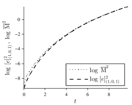
Figure 1: Example 1. The error and the majorant with respect to time.

$t^{k}$	${{\mid\mid\mid\!\nabla(u-v)\!\mid\mid\mid}^{2}_{\overline{Q}_{{t\,}^{k}}}}$	$\|\>(u-v)(x,t^{k})\>\|^{2}_{\Omega}$	${{\|\>y-\nabla v\>\|}^{2}_{\overline{Q}_{{t\,}^{k}}}}$	${{\|\>f-v_{t}+\mathrm{div}\>y\>\|}^{2}_{\overline{Q}_{{t\,}^{k}}}}$	${I_{\rm eff}^{\overline{\mathrm{M}}}}$
1.03	4.28e-04	1.52e-07	4.24e-04	2.35e-04	1.28
2.05	2.49e-03	8.44e-07	2.49e-03	1.97e-04	1.13
3.08	9.02e-03	2.94e-06	9.02e-03	1.94e-04	1.07
4.10	2.43e-02	7.70e-06	2.43e-02	1.94e-04	1.05
5.13	5.41e-02	1.68e-05	5.41e-02	2.85e-04	1.03
6.15	1.06e-01	3.25e-05	1.06e-01	2.85e-04	1.02
7.18	1.88e-01	5.71e-05	1.88e-01	2.86e-04	1.01
8.21	3.10e-01	9.38e-05	3.10e-01	1.93e-04	1.01
9.23	4.86e-01	1.46e-04	4.86e-01	3.04e-04	1.01
10.00	6.60e-01	1.97e-04	6.60e-01	2.35e-04	1.01

Table 2: Example 1. Two terms of the error, two terms of the majorant, and corresponding efficiency index with respect to time.

The normalized quantities $\frac{{[e]\,}^{2}_{(1,\>0,\>1)}}{[u]^{2}}$ and $\frac{\overline{\mathrm{M}}^{2}{}}{[u]^{2}}$ (as functions of time) are depicted in Fig. 2a. In Fig. 2b, we show the value $\frac{{[e]\,}^{2}_{(1/\sqrt{2},\>1/\sqrt{2},\>1/\sqrt{2})}}{[u]^{2}}$ and the corresponding minorant $\frac{{\underline{\mathrm{M}}^{2}}{}}{[u]^{2}}$. We see that the computed two-sided bounds of the error are efficient and guaranteed for any $t^{k}\in[0,T]$.

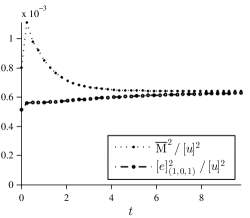
(a)

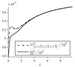
(b)

Figure 2: Example 1. (a) The relative error and majorant, (b) the relative error and minorant with respect to time.

If the weights of the error terms are selected in the special way, then the majorant and the minorant generate two-sided bounds for the same error norm (9). For any $\varkappa\in(0,2-\delta)$, we have

$$(2-\delta){\mid\!\mid\!\mid\!\nabla e\!\mid\!\mid\!\mid}^{2}+\|\>e(x,T)\>\|^{2}_{\Omega}=(2-\delta-\varkappa)\,{\mid\!\mid\!\mid\!\nabla e\!\mid\!\mid\!\mid}^{2}+\varkappa\,{\mid\!\mid\!\mid\!\nabla e\!\mid\!\mid\!\mid}^{2}+\|\>e(x,T)\>\|^{2}_{\Omega}\geq\\ (2-\delta-\varkappa)\,{\mid\!\mid\!\mid\!\nabla e\!\mid\!\mid\!\mid}^{2}+\frac{\varkappa\nu_{1}}{C_{\mathrm{F\Omega}}^{2}}\,\|\>e\>\|^{2}_{Q_{T}}+\|\>e(x,T)\>\|^{2}_{\Omega}.$$ (52)

Then, the left-hand side is estimated from above by the majorant $\overline{\mathrm{M}}^{2}{}$ (see Theorem 14) and the right-hand side is estimated from below by the minorant ${\underline{\mathrm{M}}^{2}}$ (see Theorem 34) with the corresponding weights. Henceforth, we set $\delta=1$, then weighted error norms are denoted by ${[e]\,}^{2}_{(\tilde{\nu},\,\tilde{\theta},\,\tilde{\zeta})}$, where $\tilde{\nu}=\sqrt{1-\varkappa}$, $\tilde{\theta}=\frac{\sqrt{\varkappa}}{C_{\mathrm{F\Omega}}}$, and $\tilde{\zeta}=1$. In minorant, $\kappa_{1}=2\,(1-\varkappa)$, $\kappa_{2}=\frac{2\varkappa}{C_{\mathrm{F\Omega}}^{2}}$, and $\kappa_{4}=2$. By changing $\varkappa$, we obtain different weighted norms of the error, which have computable two-sided error bounds. In Table 3, we present the efficiency index of these two-sided bounds for different $\varkappa$. In Fig. 3, we depict the behavior of $\frac{{[e]\,}^{2}_{(\tilde{\nu},\,\tilde{\theta},\,\tilde{\zeta})}}{[u]^{2}}$, $\frac{{\underline{\mathrm{M}}^{2}}{}}{[u]^{2}}$, and $\frac{\overline{\mathrm{M}}^{2}{}}{[u]^{2}}$ with respect to time for $\varkappa$ = $5\cdot 10^{\scalebox{0.5}[1.0]{$-$}1}$ and $\varkappa$ = $10^{\scalebox{0.5}[1.0]{$-$}3}$.

	$\varkappa=5\cdot 10^{\scalebox{0.5}[1.0]{$-$}1}$		$\varkappa=10^{\scalebox{0.5}[1.0]{$-$}2}$		$\varkappa=10^{\scalebox{0.5}[1.0]{$-$}3}$
$t^{k}$	${[e]\,}^{2}_{(\tilde{\nu},\,\tilde{\theta},\,\tilde{\zeta})}/[u]^{2}$	${I_{\rm eff}}=\frac{\overline{\mathrm{M}}}{\underline{\mathrm{M}}}$	${[e]\,}^{2}_{(\tilde{\nu},\,\tilde{\theta},\,\tilde{\zeta})}/[u]^{2}$	${I_{\rm eff}}=\frac{\overline{\mathrm{M}}}{\underline{\mathrm{M}}}$	${[e]\,}^{2}_{(\tilde{\nu},\,\tilde{\theta},\,\tilde{\zeta})}/[u]^{2}$	${I_{\rm eff}}=\frac{\overline{\mathrm{M}}}{\underline{\mathrm{M}}}$
0.26	2.95e-04	3.02	5.10e-04	1.69	5.14e-04	1.69
1.03	2.98e-04	3.36	5.58e-04	1.69	5.63e-04	1.68
2.05	2.91e-04	2.60	5.66e-04	1.31	5.71e-04	1.30
3.08	2.95e-04	2.31	5.79e-04	1.17	5.85e-04	1.16
4.10	3.01e-04	2.19	5.91e-04	1.11	5.96e-04	1.10
5.13	3.05e-04	2.13	6.00e-04	1.08	6.05e-04	1.07
6.15	3.08e-04	2.10	6.07e-04	1.06	6.12e-04	1.05
7.18	3.11e-04	2.08	6.12e-04	1.05	6.18e-04	1.04
8.21	3.13e-04	2.06	6.16e-04	1.04	6.22e-04	1.03
9.23	3.15e-04	2.05	6.20e-04	1.04	6.25e-04	1.03
10.00	3.16e-04	2.04	6.22e-04	1.03	6.27e-04	1.02

Table 3: Example 1. The error and efficiency index ${I_{\rm eff}}=\frac{\overline{\mathrm{M}}}{\underline{\mathrm{M}}}$ with respect to time for different parameter $\varkappa$.

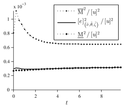
(a)

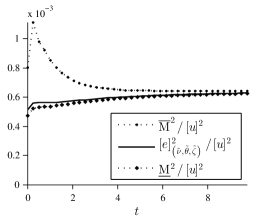
(b)

Figure 3: Example 1. Two-sided bounds of the error with respect to time for (a) $\varkappa=10^{-1}$ and (b) $\varkappa=5\cdot 10^{-3}$.

The efficiency of the majorant (minorant) depends on the selection of $y\in Y_{\mathrm{div}\>}(Q_{T})$ $\left(\eta\in{\mathring{H}}^{1}(Q_{T})\right)$. For elliptic problems, this question is well studied, and there exist methods which are able to reconstruct $y$ using the computed flux $A\nabla v$ (see, e.g., [18, 20, 5]). We follow the same technique and obtain a suitable $y$ ($\eta$) by local minimization of $\overline{\mathrm{M}}^{2}{}$ (maximization of ${\underline{\mathrm{M}}^{2}}$). The corresponding results are collected in Table 4. The first two columns show the performance of $\overline{\mathrm{M}}^{2}{}$ with the most coarse reconstruction, in which $y$ is obtained by a simple patch-wise averaging of the numerical flux $A\nabla v$. This procedure is very cheap and does not lead to noticeable computational costs. The columns 5 and 6 show the estimates obtained after minimization process, in which $y$ was computed by means of a patch-wise minimization of $\overline{\mathrm{M}}^{2}{}$. The last two columns present the results related to the best possible reconstruction of the flux obtained by adding patch-wise based bubble functions. Table 5 presents analogous results for the minorant, which were obtained by computing integrals in (34) on each time-step cylinder.

$t^{k}$	${[e]\,}^{2}_{(1,\>0,\>1)}$	$\overline{\mathrm{M}}^{2}{}\left(y\right)$	${I_{\rm eff}^{\overline{\mathrm{M}}}}$	$\overline{\mathrm{M}}^{2}{}\left(y^{opt}\right)$	${I_{\rm eff}^{\overline{\mathrm{M}}}}$	$\overline{\mathrm{M}}^{2}{}\left(y^{opt}_{ref}\right)$	${I_{\rm eff}^{\overline{\mathrm{M}}}}$
1.03	5.64e-04	4.97e-03	2.97	9.49e-04	1.30	9.22e-04	1.28
2.05	5.71e-04	3.87e-03	2.60	7.43e-04	1.14	7.35e-04	1.13
3.08	5.85e-04	3.19e-03	2.34	6.78e-04	1.08	6.75e-04	1.07
4.10	5.97e-04	2.73e-03	2.14	6.55e-04	1.05	6.53e-04	1.05
5.13	6.06e-04	2.41e-03	1.99	6.45e-04	1.03	6.45e-04	1.03
6.15	6.13e-04	2.17e-03	1.88	6.43e-04	1.02	6.43e-04	1.02
7.18	6.18e-04	1.99e-03	1.79	6.42e-04	1.02	6.42e-04	1.02
8.21	6.22e-04	1.84e-03	1.72	6.41e-04	1.02	6.41e-04	1.01
9.23	6.26e-04	1.73e-03	1.66	6.41e-04	1.01	6.41e-04	1.01
10.00	6.28e-04	1.65e-03	1.62	6.41e-04	1.01	6.41e-04	1.01

Table 4: Example 1. Minimization of the majorant $\overline{\mathrm{M}}^{2}{}$ with respect to flux on every time-cylinder $Q^{k}$, $k=1,...,39$.

$t^{k}$	${[e]\,}^{2}_{(1/\sqrt{2},\>1/\sqrt{2},\>1/\sqrt{2})}$	${\underline{\mathrm{M}}^{2}}\left(\eta\right)$	${I_{\rm eff}^{\underline{\mathrm{M}}}}$	${\underline{\mathrm{M}}^{2}}\left(\eta^{opt}\right)$	${I_{\rm eff}^{\underline{\mathrm{M}}}}$
1.03	5.64e-04	4.29e-04	0.87	5.09e-04	0.99
2.05	5.71e-04	5.11e-04	0.95	5.22e-04	1.00
3.08	5.85e-04	5.34e-04	0.96	5.36e-04	1.00
4.10	5.97e-04	5.46e-04	0.96	5.47e-04	1.00
5.13	6.06e-04	5.54e-04	0.96	5.55e-04	1.00
6.15	6.13e-04	5.60e-04	0.96	5.60e-04	1.00
7.18	6.18e-04	5.65e-04	0.96	5.65e-04	1.00
8.21	6.22e-04	5.68e-04	0.96	5.68e-04	1.00
9.23	6.26e-04	5.71e-04	0.96	5.71e-04	1.00
10.00	6.28e-04	5.73e-04	0.96	5.73e-04	1.00

Table 5: Example 1. Maximization of the minorant ${\underline{\mathrm{M}}^{2}}{}$ with respect to $\eta$ on every time-cylinder $Q^{k}$, $k=1,...,39$.

For the next set of numerical tests, we assume that the reaction term is positive and behaves as the Gaussian function, i.e.,

$$\lambda(x)=\frac{1}{\sigma_{\lambda}\sqrt{2\pi}}\exp\left(\frac{-\left(x-\frac{1}{2}\right)^{2}}{2\,\sigma_{\lambda}^{2}}\right).$$ (53)

Then, the right-hand side of the problem is changed to $f=x\,(1-x)\,(2t+1)+(\lambda\,x\,(1-x)+2)\,(t^{2}+t+1)$. From Fig. 4, we see that for the certain $\sigma_{\lambda}$ the reaction $\lambda$ changes rapidly from very small values (in one part of $\Omega$) to relatively big values (in another part). The estimate (14) was derived specially for such type cases, and we use this example in order to verify it. Consider a simplified form of (14) with $\delta=1$ and $\beta={\rm const}$, which implies the majorant

$$\overline{\mathrm{M}}^{2}_{(\mu)}(v,y):=\|\,e(0,x)\,\|^{2}_{\Omega}+\int\limits_{0}^{T}\Bigg{(}\gamma\bigg{\|}\,\frac{\mu}{\sqrt{\lambda}}\,\mathscr{R}_{f}(v,y)\,\bigg{\|}^{2}_{\Omega}\>+\bigg{(}1+\frac{1}{\beta}\bigg{)}C_{\mathrm{F\Omega}}^{2}\|\,(1-\mu)\,\mathscr{R}_{f}(v,y)\,\|^{2}_{\Omega}\>+(1+\beta)\|\,\mathscr{R}_{d}(v,y)\,\|^{2}_{A^{\scalebox{0.5}[1.0]{$-$}1}}\Bigg{)}\mathrm{\>d}t=\\ \|\,e(0,x)\,\|^{2}_{\Omega}+\int\limits_{Q_{T}}\Bigg{(}\gamma\frac{\mu^{2}}{\lambda}\,\mathscr{R}^{2}_{f}(v,y)\,\>+\bigg{(}1+\frac{1}{\beta}\bigg{)}C_{\mathrm{F\Omega}}^{2}(1-\mu)^{2}\,\mathscr{R}^{2}_{f}(v,y)\>+(1+\beta)\mathscr{R}^{2}_{d}(v,y)\Bigg{)}\mathrm{\>d}x\mathrm{\>d}t.$$ (54)

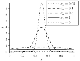
Figure 4: The reaction term $\lambda(x)$ defined by (53) .

Minimization of the right-hand side of (54) with respect to $\mu$ is reduced to the auxiliary variational problem: find $\hat{\mu}\in L^{\infty}(\Omega)$ such that

$$\Upsilon(\hat{\mu})=\!\!\inf\limits_{\mu\>\in\>L^{\infty}(\Omega)}\!\!\!\Upsilon(\mu),\quad\mbox{for a.e.}\quad t\in(0,T),$$ (55)

where

$$\Upsilon(\mu):=\int\limits_{Q_{T}}\Bigg{(}\gamma\frac{\mu^{2}}{\lambda}\,\mathscr{R}^{2}_{f}(v,y)\,\>+\bigg{(}1+\frac{1}{\beta}\bigg{)}C_{\mathrm{F\Omega}}^{2}(1-\mu)^{2}\,\mathscr{R}^{2}_{f}(v,y)\Bigg{)}\mathrm{\>d}x\mathrm{\>d}t.$$ (56)

It is easy to find that for a.e. $(x,t)\in Q_{T}$ the minimizer satisfies the condition

$$\hat{\mu}(x,t)=\frac{C_{\mathrm{F\Omega}}^{2}(1+\beta)\lambda}{\beta\gamma+C_{\mathrm{F\Omega}}^{2}(1+\beta)\lambda}.$$ (57)

Table 6 shows the efficiency of $\overline{\mathrm{M}}^{2}_{(\hat{\mu})}$ and $\overline{\mathrm{M}}^{2}_{(0)}$ for different $\sigma_{\lambda}$. In the left part of it, the results correspond to the case where $y$ is reconstructed by piecewise affine approximations, and in the right part we expose the results obtained if $y$ is taken from a reacher space (which includes piecewise quadratic functions). We see that $\overline{\mathrm{M}}^{2}_{(0)}$ grows dramatically if $\sigma_{\lambda}$ goes to zero, while $\overline{\mathrm{M}}^{2}_{(\hat{\mu})}$ keeps small values of the efficiency index for all $\sigma_{\lambda}$. In other words, $\overline{\mathrm{M}}^{2}_{(\hat{\mu})}$ stays efficient and robust even if the reaction function changes its values quite drastically in different parts of the domain.

	$y_{opt}$ (linear approximation)			$y^{ref}_{opt}$ (quadratic approximation)
$\sigma_{\lambda}$	${I_{\rm eff}^{\overline{\mathrm{M}}_{(0)}}}$	${I_{\rm eff}^{\overline{\mathrm{M}}_{(\hat{\mu})}}}$		${I_{\rm eff}^{\overline{\mathrm{M}}_{(0)}}}$	${I_{\rm eff}^{\overline{\mathrm{M}}_{(\hat{\mu})}}}$
0.05	$9.037\cdot 10^{8}$	1.0080		$9.037\cdot 10^{8}$	1.0077
0.10	2.4416	1.0063		2.4282	1.0061
0.50	1.0020	1.0017		1.0020	1.0017
1.00	1.0035	1.0029		1.0034	1.0027
5.00	1.0173	1.0079		1.0168	1.0075

Table 6: Example 1. Efficiency indexes for different values of $\sigma_{\lambda}$ for $t=T$.

Example 2

Consider the same problem as in Example 1 but with $\varphi=x\,\sin\!\left(3\,\pi\,x\right)$, $A=I$, $\lambda(x,t)=\rho\,(t^{2}+1)(x+10^{\scalebox{0.5}[1.0]{$-$}3})$, where $\rho$ is a positive constant, and $f=\mathrm{e}^{t}\,\left(x\,(1+9\pi^{2})\sin\!\left(3\,\pi\,x\right)-6\,\pi\,\cos\!\left(3\,\pi\,x\right)\right)+\lambda(x,t)\sin(3\,\pi\,x)\,\mathrm{e}^{t}$. The exact solution is $u=x\,\sin\!\left(3\,\pi\,x\right)\,\mathrm{e}^{t}$.

Table 7 presents the efficiency of $\overline{\mathrm{M}}^{2}_{(\hat{\mu})}$, $\overline{\mathrm{M}}^{2}_{(1)}$ and $\overline{\mathrm{M}}^{2}_{(0)}$ for different $\rho$. It shows that $\overline{\mathrm{M}}^{2}_{(\hat{\mu})}$ always provides accurate upper bound of the error, whereas $\overline{\mathrm{M}}^{2}_{(1)}$ and $\overline{\mathrm{M}}^{2}_{(0)}$ may overestimate it if $\rho$ is sufficiently small or large. Fig. 5 illustrates the same behavior of $\overline{\mathrm{M}}^{2}_{(\hat{\mu})}$, $\overline{\mathrm{M}}^{2}_{(1)}$, and $\overline{\mathrm{M}}^{2}_{(0)}$ with respect to $\log\,\rho$. These results confirm that $\overline{\mathrm{M}}^{2}_{(\hat{\mu})}$ is indeed robust and have serious advantages in the case where $\lambda$ may attain quite different value (very small and very large) in different parts of the domain.

	$y_{opt}$ (linear approximation)				$y^{ref}_{opt}$ (quadratic approximation)
$\rho$	${I_{\rm eff}^{\overline{\mathrm{M}}_{(1)}}}$	${I_{\rm eff}^{\overline{\mathrm{M}}_{(0)}}}$	${I_{\rm eff}^{\overline{\mathrm{M}}_{(\hat{\mu})}}}$		${I_{\rm eff}^{\overline{\mathrm{M}}_{(1)}}}$	${I_{\rm eff}^{\overline{\mathrm{M}}_{(0)}}}$	${I_{\rm eff}^{\overline{\mathrm{M}}_{(\hat{\mu})}}}$
$10^{\scalebox{0.5}[1.0]{$-$}3}$	3.5751	94.0962	3.5692		2.6520	60.1361	2.6477
$10^{\scalebox{0.5}[1.0]{$-$}2}$	3.5835	29.8481	3.5272		2.6610	19.0925	2.6196
$10^{\scalebox{0.5}[1.0]{$-$}1}$	3.6209	9.6446	3.2145		2.7011	6.2272	2.4205
$10^{0}$	3.3249	2.8622	2.1385		2.7018	2.1808	1.9152
$10^{1}$	4.4795	1.2291	1.2608		4.2507	1.2200	1.2608
$10^{2}$	11.7222	1.0795	1.0787		11.2044	1.0795	1.0787
$10^{3}$	37.6760	1.0622	1.0622		36.4553	1.0622	1.0622
$10^{3}$	37.6760	1.0622	1.0622		36.4553	1.0622	1.0622

Table 7: Example 2. Efficiency indexes for different values of $\rho$ for $t=T$.

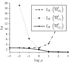
Figure 5: Example 2. Efficiency indexes of the majorants $\overline{\mathrm{M}}^{2}_{(1)}$, $\overline{\mathrm{M}}^{2}_{(0)}$, and $\overline{\mathrm{M}}^{2}_{(\hat{\mu})}$ for different constant $\log\rho$.

Example 3

We set $\Omega=(0,1)$, $T$ = 10, and consider the problem with mixed Dirichlet–Neumann boundary conditions, namely, $u(0,t)=0$ and $u^{\prime}(1,t)=0$, and

$$f \;=x\,\Big{(}\cos\!\left(t\right)-\sin\!\left(t\right)\Big{)}\,{\left(x-1\right)}^{2}-2\Big{(}\cos\!\left(t\right)+\sin\!\left(t\right)\Big{)}\,\Big{(}3\,x-2\Big{)},$$

$$\varphi \;=\sin\!\left(\pi\,x\right)\,\Big{(}\cos\!\left(\pi\,x\right)+1\Big{)},$$

$${\lambda} \;=0.$$ (58)

The exact solution is $u(x,t)=\sin\!\left(\pi\,x\right)\,\left(t\,\cos\!\left(t\right)+1\right)\,\left(\cos\!\left(\pi\,x\right)+1\right)$.

Table 8 shows the relative error $\frac{{[e]\,}^{2}_{(1,\>0,\>1)}}{[u]^{2}}$, the majorant $\frac{\overline{\mathrm{M}}^{2}{}}{[u]^{2}}$, and the efficiency index for different meshes, where $N_{1}$ denotes the amount of intervals with respect to the space coordinate $x$ and $K$ with respect to the time $t$. We can see that the efficiency index stays on the approximately same level for all considered meshes, therefore the majorant does not deteriorate in the process of mesh refining. It is worth remarking that results exposed in Table 8 are quite typical, and similar behavior of the error majorant was observed in many other numerical tests.

$N_{1}$	$K$	${[e]\,}^{2}_{(1,\>0,\>1)}\,/\,[u]^{2}$	$\overline{\mathrm{M}}^{2}{}\,/\,[u]^{2}$	${I_{\rm eff}^{\overline{\mathrm{M}}}}$
20	20	6.41e-03	2.23e-02	1.87
20	40	5.87e-03	2.27e-02	1.96
20	80	5.88e-03	2.26e-02	1.96
20	160	5.89e-03	2.27e-02	1.96
40	40	1.37e-03	5.14e-03	1.94
40	80	1.34e-03	5.04e-03	1.94
40	160	1.34e-03	5.14e-03	1.95
80	80	3.26e-04	1.22e-03	1.93

Table 8: Example 3. The relative error, majorant, and its efficiency index with respect to different meshes $\Theta{\>K\times N_{1}}$ for $t=T$.

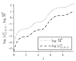
Figure 6: Example 3. The logarithm of the error and majorant with respect to time.

In Fig. 6, we depict growth of the error and majorant in the logarithmic scale (for mesh $\Theta_{\>K\times N_{1}}$ = $\Theta_{\>40\times 40}$). The gap between two curves reflects the impact of the term ${\overline{\mathrm{m}}}^{2}_{\mathrm{f}}$ (see Table 9) and corresponds to the efficiency index ${I_{\rm eff}^{\overline{\mathrm{M}}}}\approx 1.87,\ldots,1.96$. The efficiency of the majorant can be improved by choosing higher order approximations for the flux reconstruction (e.g., we can add element-wise based bubble functions; corresponding results are presented in columns 7 and 8 of Table 10). Table 10 illustrates minimization of $\overline{\mathrm{M}}^{2}{}$ with respect to $y$ and corresponding efficiency indexes on every local time-cylinder $Q^{k}$. For example, consider the row of Table 10 related to $t_{k}=6.15$. The corresponding error ${[e]\,}^{2}_{(1,\>0,\>1)}=1.33e\scalebox{0.5}[1.0]{$-$}03$ and the estimate provided by the majorant with a simple (patch averaging) reconstruction of the flux is $\overline{\mathrm{M}}^{2}=6.42e\scalebox{0.5}[1.0]{$-$}03$ $\left({I_{\rm eff}^{\overline{\mathrm{M}}}}=2.20\right)$. If we apply a more sophisticated procedure and reconstruct flux by minimizing the majorant with respect to values of $y$ associated with the given spatial mesh on the time-layer $t_{k}=6.15$, then we obtain the efficiency index ${I_{\rm eff}^{\overline{\mathrm{M}}}}=2.18$. If we use a twice finer spacial mesh, then the index decreases up to $1.90$. Obtained results show that for this particular example simple flux reconstructions generate sufficiently accurate estimates.

It is worth noting that, in general, the efficiency of the majorant depends on the several factors. First, it can be improved by using advanced reconstructions of the flux (e.g., by adding extra degrees of freedom, bubble functions, etc). However, this approach may lead to a limited effect, if approximations are coarse with respect to the time variable and/or the time steps are large (the term $v_{t}$ in the balancing term may be a piecewise constant function, which cannot reflect the behavior of $f$).

$t^{k}$	${{\mid\mid\mid\!\nabla(u-v)\!\mid\mid\mid}^{2}_{\overline{Q}_{{t\,}^{k}}}}$	$\|\>(u-v)(x,t^{k})\>\|^{2}_{\Omega}$	${{\|\>y-\nabla v\>\|}^{2}_{\overline{Q}_{{t\,}^{k}}}}$	${{\|\>f-v_{t}+\mathrm{div}\>y\>\|}^{2}_{\overline{Q}_{{t\,}^{k}}}}$
1.03	8.72e-03	1.42e-04	8.37e-03	7.48e-02
2.05	6.00e-04	4.40e-06	5.02e-04	7.71e-03
3.08	1.29e-02	2.15e-04	1.24e-02	1.11e-01
4.10	1.12e-02	1.62e-04	1.01e-02	1.02e-01
5.13	2.07e-02	3.16e-04	2.07e-02	1.87e-01
6.15	1.62e-01	2.53e-03	1.60e-01	1.38e+00
7.18	1.30e-01	2.00e-03	1.27e-01	1.11e+00
8.21	3.36e-03	3.14e-05	3.35e-03	5.98e-02
9.23	2.05e-01	3.10e-03	2.00e-01	1.75e+00
10.00	2.22e-01	3.33e-03	2.14e-01	1.90e+00

Table 9: Example 3. Two terms of the error and two terms of the majorant with respect to time.

$t^{k}$	${[e]\,}^{2}_{(1,\,0,\,1)}$	$\overline{\mathrm{M}}^{2}{}(y)$	${I_{\rm eff}^{\overline{\mathrm{M}}}}$	$\overline{\mathrm{M}}^{2}{}(y^{opt})$	${I_{\rm eff}^{\overline{\mathrm{M}}}}$	$\overline{\mathrm{M}}^{2}{}(y^{opt}_{ref})$	${I_{\rm eff}^{\overline{\mathrm{M}}}}$
1.03	1.33e-03	6.58e-03	2.22	6.50e-03	2.21	4.79e-03	1.90
2.05	1.46e-03	5.31e-03	1.91	5.31e-03	1.91	5.25e-03	1.90
3.08	1.38e-03	6.10e-03	2.11	6.05e-03	2.10	4.98e-03	1.90
4.10	1.47e-03	5.74e-03	1.98	5.73e-03	1.97	5.27e-03	1.89
5.13	1.42e-03	5.93e-03	2.04	5.89e-03	2.04	5.15e-03	1.91
6.15	1.33e-03	6.42e-03	2.20	6.36e-03	2.18	4.81e-03	1.90
7.18	1.40e-03	5.65e-03	2.01	5.63e-03	2.01	5.03e-03	1.90
8.21	1.43e-03	5.16e-03	1.90	5.16e-03	1.90	5.15e-03	1.90
9.23	1.39e-03	5.67e-03	2.02	5.65e-03	2.02	5.01e-03	1.90
10.00	1.41e-03	5.58e-03	1.99	5.56e-03	1.99	5.06e-03	1.90

Table 10: Example 3. Minimization of the majorant $\overline{\mathrm{M}}^{2}{}$ with respect to flux on every time-cylinder $Q^{k}$, $k=1,...,39$.

Now, we shortly discuss results related to error indicators generated by the majorant, which can be represented in the form

$$\overline{\mathrm{M}}^{2}{}(v,y,\beta):=\|\,e(x,0)\,\|^{2}_{\Omega}+\frac{1}{\delta}\int\limits_{0}^{T}\Bigg{(}\big{(}1+\beta\big{)}\overline{\mathrm{m}}^{2}_{\mathrm{d}}+\bigg{(}1+\frac{1}{\beta}\bigg{)}\,C_{\mathrm{F\Omega}}^{2}\overline{\mathrm{m}}^{2}_{\mathrm{f}}\Bigg{)}\mathrm{\>d}t,$$ (59)

where

$$\overline{\mathrm{m}}^{2}_{\mathrm{d}}=\|\>y-\nabla v\>\|^{2}_{\Omega},\quad\overline{\mathrm{m}}^{2}_{\mathrm{f}}=\|\>f-v_{t}-\lambda v+\mathrm{div}\>y\>\|^{2}_{\Omega}.$$ (60)

The ‘reliability term’ $\overline{\mathrm{m}}^{2}_{\mathrm{f}}$ is necessary to provide a guaranteed upper bound, but the major part of the error is usually encompassed in $\overline{\mathrm{m}}^{2}_{\mathrm{d}}$. The conclusion, which follows from our experience is that the term $\overline{\mathrm{m}}^{2}_{\mathrm{d}}$ (which is an integral over $\Omega$) can be considered as an efficient indicator of element-wise error. Fig. 7 presents distribution of the error indicator $\overline{\mathrm{m}}^{2}_{\mathrm{d}}$ and error over time-step cylinder $Q_{30}$ (for zero reaction function). Assume now that $\lambda(x)=\frac{1}{\sigma_{\lambda}\sqrt{2\pi}}\exp\left(\frac{-\left(x-\frac{1}{2}\right)^{2}}{2\,\sigma_{\lambda}^{2}}\right)$ (which correspondingly changes $u$ and $f$) with $\sigma_{\lambda}$ = 0.05 and $\sigma_{\lambda}$ = 0.1. Fig. 8 illustrates typical results related to different $\sigma_{\lambda}$ and time-cylinder $Q_{30}$.

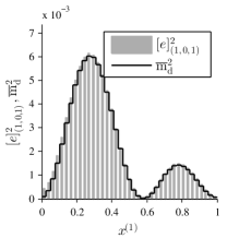
Figure 7: Example 3. The distribution of the local errors and indicator $\overline{\mathrm{m}}^{2}_{\mathrm{d}}{}$ for time-layers $Q^{30}$.

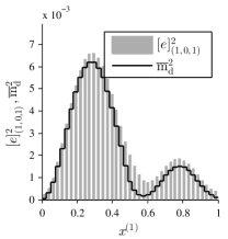
(a) $\sigma_{\lambda}$ = 0.05, $Q^{30}$

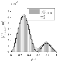
(b) $\sigma_{\lambda}$ = 0.1, $Q^{30}$

Figure 8: Example 3. The error and indicator for time-layers $Q^{30}$ for $\sigma_{\lambda}$ = 0.05 and $\sigma_{\lambda}$ = 0.1.

Example 4

Consider the problem $\Omega=[0,1]\times[0,1]\in{\mathds{R}}^{2}$, $T=1$, and homogeneous Dirichlet boundary condition, $\varphi(x)=\sin\!\left(\pi\,x\right)\,\sin\!\left(3\,\pi\,y\right)+\sin\!\left(3\,\pi\,x\right)\,\sin\!\left(\pi\,y\right)$, $A=I$, and

$$f=\Big{(}\sin\!\left(\pi\,x\right)\,\sin\!\left(3\,\pi\,y\right)+\sin\!\left(3\,\pi\,x\right)\,\sin\!\left(\pi\,y\right)\Big{)}\,\Big{(}\cos\!\left(t\right)+10\,{\pi}^{2}\,\sin\!\left(t\right)+10\,{\pi}^{2}\,t^{3}+3\,t^{2}+10\,{\pi}^{2}\Big{)}.$$ (61)

The corresponding exact solution $u=\Big{(}\sin(\pi x)\sin(3\pi y)+\sin(\pi y)\sin(3\pi x)\Big{)}\Big{(}t^{3}+\sin(t)+1\Big{)}$ is a rapidly changing function.

In Table 11, we compare $\frac{{[e]\,}^{2}_{(1,\,0,\,1)}}{[u]^{2}}$ with $\frac{\overline{\mathrm{M}}^{2}{}}{[u]^{2}}$ and its efficiency index (for the approximate solution computed on the mesh $\Theta_{\>K\times N_{1}\times N_{2}}$ = $\Theta_{\>100\times 50\times 50}$). We can see that the majorant based on ‘cheap’ (local patch averaging) reconstruction of the flux $y=G(\nabla v)$ provides a quite realistic upper bound of the error. However, in more complicated problems an optimization of the majorant with respect to $y$ may be useful. This procedure yields sharper upper bounds but requires more computational efforts (concerning the corresponding methods based on multigrid, isogeometric elements, and other methods, see [20, 5, 9]).

$t^{k}$	${[e]\,}^{2}_{(1,\,0,\,1)}/[u]^{2}$	$\overline{\mathrm{M}}^{2}{}(G(\nabla v))/[u]^{2}$	${I_{\rm eff}^{\overline{\mathrm{M}}}}$
0.10	2.58e-03	2.56e-02	3.15
0.20	2.70e-03	2.68e-02	3.15
0.30	2.74e-03	2.72e-02	3.15
0.40	2.76e-03	2.74e-02	3.15
0.51	2.78e-03	2.75e-02	3.15
0.60	2.79e-03	2.76e-02	3.15
0.70	2.79e-03	2.77e-02	3.15
0.80	2.80e-03	2.78e-02	3.15
0.90	2.81e-03	2.79e-02	3.15
1.00	2.82e-03	2.80e-02	3.15

Table 11: Example 4. The relative true error and relative majorant with respect to time.

Next goal is to investigate the accuracy of the error indicator defined in (59)–(60). We analyze two different measures, which can be called ‘weak’ and ‘strong’ and are discussed in details in [9]. The first measure is studied in the context of a certain marking procedure $\mathbb{M}$, which maps element-wise error into a boolean array, i.e., it deals with the values $0$ and $1$ only. The corresponding ‘weak’ measure $\mathcal{M}_{\rm weak}\in[0,1]$ is defined by the percentage of correctly marked elements.

Another measure compares element-wise values of the true error and estimates of local errors generated by the error indicator. For $\overline{\mathrm{m}}^{2}_{\mathrm{d}}{}$, it is defined by the relation

$$\mathcal{M_{\rm str}}(\overline{\mathrm{m}}^{2}_{\mathrm{d}}{}):=\frac{\big{|}{[e]\,}^{2}_{(1,\>0,\>1)}-\overline{\mathrm{m}}^{2}_{\mathrm{d}}{}\big{|}}{\big{|}{[e]\,}^{2}_{(1,\>0,\>1)}\big{|}}.$$ (62)

To analyze the quality of the weak measure, we consider bulk marking procedure $\mathbb{M}_{\theta}$, where $\theta\in(0,1)$ (see, e.g., [2]). Fig. 9 illustrates $\mathbb{M}_{\theta}$ for $\theta$ = 0.2 and 0.4 (it has been performed for the actual error and for the error indicator $\overline{\mathrm{m}}^{2}_{\mathrm{d}}{}$). The results obtained for the error (Fig. 9 left) and for the indicator (right) are almost identical. We also have obtained quite small values of the weak error measure for bulk parameters $\theta$ = 0.2, 0.3, and 0.4:

$$\mathcal{M_{\rm weak}}(\mathbb{M}_{0.2})=5.83e\scalebox{0.5}[1.0]{$-$}03,\quad\mathcal{M_{\rm weak}}(\mathbb{M}_{0.3})=4.58e\scalebox{0.5}[1.0]{$-$}03,\quad\mbox{and}\quad\mathcal{M_{\rm weak}}(\mathbb{M}_{0.4})=1.41e\scalebox{0.5}[1.0]{$-$}02.$$ (63)

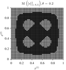
(a)

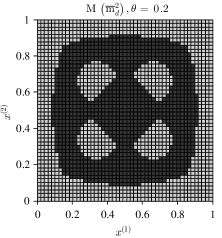
(b)

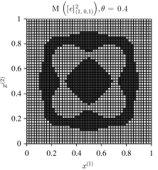
(c)

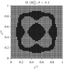
(d)

Figure 9: Example 4. ’Bulk’ marking for $\theta$ = 0.2 and 0.4 based on the true error ${[e]\,}^{2}_{(1,\,0,\,1)}$ (left) and the indicator $\overline{\mathrm{m}}^{2}_{\mathrm{d}}{}(G(\nabla v))$ for $Q^{40}$.

To understand whether or not the error indicator is quantitatively sharp and reproduces the error distribution accurately, we consider the histograms depicted in Fig. 10, which are constructed by the procedure suggested in [9]. We assume that all element-wise errors are ranked in the decreasing order with respect to values of the true error distribution ${[e]\,}^{2}_{(1,\,0,\,1)}$, and renumber all the elements accordingly, so that the element with the largest error is numbered 1. Then, we depict errors in this new order. The distribution of the element-wise errors generated by $\overline{\mathrm{m}}^{2}_{\mathrm{d}}{}$ is depicted in the same way. In Fig. 10, we consider true and indicated error distributions (the approximation computed on a regular mesh with 2 500 elements). If $\overline{\mathrm{m}}^{2}_{\mathrm{d}}{}$ is accurate in the strong sense, then the corresponding histogram (on the right) must resemble the histogram generated by the true error. Therefore, Fig. 10 shows that in this example the indicator is indeed sharp in the strong sense.

(a)

(b)

Figure 10: Example 4. Histograms of the ranked element-wise errors and indicator by $\overline{\mathrm{m}}^{2}_{\mathrm{d}}{}$ for $Q^{40}$ (2 500 elements).

Example 5

Finally, we test the example, in which the exact solution essentially changes both in space and time. Here, $\Omega=[0,1]\times[0,1]$, $T=10$, $\partial\Omega=\Gamma_{D}$, $u=0$ on $S_{D}$, and $\varphi(x)=\sin\!\left(\pi\,x\right)\,\sin\!\left(2\,\pi\,y\right)+\sin\!\left(2\,\pi\,x\right)\,\sin\!\left(\pi\,y\right)$, $A=I$, and

$$f=\sin\!\left(2\,\pi\,x\right)\,\sin\!\left(\pi\,y\right)\,\bigg{(}\cos\!\left(t\right)-\sin\!\left(t\right)+5\,{\pi}^{2}\,\Big{(}\cos\!\left(t\right)+\sin\!\left(t\right)\Big{)}\bigg{)}\,+\\ \sin\!\left(\pi\,x\right)\,\sin\!\left(2\,\pi\,y\right)\,\bigg{(}\sin\!\left(t\right)+t\,\cos\!\left(t\right)+5\,{\pi}^{2}\,\Big{(}t\,\sin\!\left(t\right)+1\Big{)}\bigg{)}.$$ (64)

The exact solution is $u=\sin\!\left(\pi\,x\right)\,\sin\!\left(2\,\pi\,y\right)\,\left(t\,\sin\!\left(t\right)+1\right)+\sin\!\left(2\,\pi\,x\right)\,\sin\!\left(\pi\,y\right)\,\left(\cos\!\left(t\right)+\sin\!\left(t\right)\right)$.

We investigate the efficiency of bulk marking for $\theta$ = 0.5 and different time-layers for approximate solution constructed on the mesh $\Theta_{\>K\times N_{1}\times N_{2}}=\Theta_{\>200\times 50\times 50}$ (see Fig. 11). Here,

$$\mathcal{M_{\rm weak}}(\mathbb{M}_{\rm 0.5})=5.08e\scalebox{0.5}[1.0]{$-$}02\;\;\mbox{for}\;\;Q^{40},\quad\mathcal{M_{\rm weak}}(\mathbb{M}_{\rm 0.5})=5.4e\scalebox{0.5}[1.0]{$-$}02\;\;\mbox{for}\;\;Q^{80},\quad\mbox{and}\;\;\mathcal{M_{\rm weak}}(\mathbb{M}_{\rm 0.5})=3.70e\scalebox{0.5}[1.0]{$-$}02\;\;\mbox{for}\;\;Q^{160}.$$

The histograms from Fig. 12 are constructed by the same method as in the previous example (for 2 500 elements). They confirm quantitative efficiency of $\overline{\mathrm{m}}^{2}_{\mathrm{d}}{}$ . Again, we see that the majorant provides an efficient estimation of the global error as well as indication of element-wise errors. In this and also other experiments, we have observed that the quality of error estimation is good if the solution is smooth in space and rather monotonic in time, and it becomes less accurate if the solution admits large gradients with respect to the spacial variables and large time derivatives. In our experiments, this was mainly due to rather coarse (piecewise affine) approximations in time used for $v$ and $y$. This fact constrains accuracy of the error estimation (especially in the context of the reliability term $\overline{\mathrm{m}}^{2}_{\mathrm{f}}$). However, choosing richer spaces for the reconstruction of $v$ and $y$ will lead to sharper estimates.

(a) $t^{k}$ = 2.06

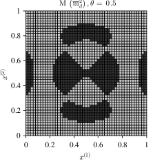
(b) $t^{k}$ = 2.06

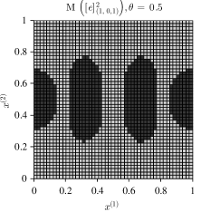
(c) $t^{k}$ = 4.07

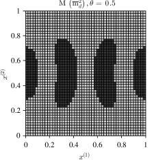
(d) $t^{k}$ = 4.07

(e) $t^{k}$ = 8.04

(f) $t^{k}$ = 8.04

Figure 11: Example 5. ’Bulk’ marking ($\theta=0.5$) based on the true error ${[e]\,}^{2}_{(1,\>0,\>1)}$ (left) and indicator $\overline{\mathrm{m}}^{2}_{\mathrm{d}}{}(y=G(\nabla v))$ (right) for $Q^{40}$, $Q^{80}$, and $Q^{80}$.

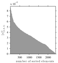
(a) $t^{k}$ = 2.06

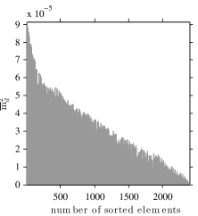
(b) $t^{k}$ = 2.06

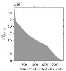
(c) $t^{k}$ = 4.07

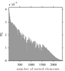
(d) $t^{k}$ = 4.07

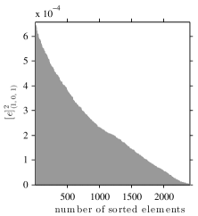
(e) $t^{k}$ = 8.04

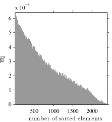
(f) $t^{k}$ = 8.04

Figure 12: Example 5. Histograms of the ranked element-wise errors and error indicator by $\overline{\mathrm{m}}^{2}_{\mathrm{d}}{}$ for $Q^{40}$, $Q^{80}$, and $Q^{80}$.

References

[1]
D. Braess.
Finite elements.
Cambridge University Press, Cambridge, second edition, 2001.
Theory, fast solvers, and applications in solid mechanics, Translated
from the 1992 German edition by Larry L. Schumaker.
[2]
W. Dörfler.
A convergent adaptive algorithm for Poisson’s equation.
SIAM J. Numer. Anal., 33(3):1106–1124, 1996.
[3]
L. C. Evans.
Partial differential equations, volume 19 of Graduate
Studies in Mathematics.
American Mathematical Society, Providence, RI, second edition, 2010.
[4]
C. Johnson.
Numerical solution of partial differential equations by the
finite element method.
Dover Publications Inc., Mineola, NY, 2009.
Reprint of the 1987 edition.
[5]
S. Kleiss and S. Tomar.
Guaranteed and sharp a posteriori error estimates in isogeometric
analysis.
Technical Report v2, Johann Radon Institute for Computational and
Applied Mathematics (RICAM), Austrian Academy of Sciences, Altenberger
Straße 69, A-4040 Linz, Austria, 2013.
[6]
O. A. Ladyzhenskaya.
The boundary value problems of mathematical physics.
Springer, New York, 1985.
[7]
O. A. Ladyzhenskaya, V. A. Solonnikov, and N. Uraltseva.
Linear and quasilinear equations of parabolic type.
Nauka, Moscow, 1967.
[8]
R. J. LeVeque.
Finite difference methods for ordinary and partial differential
equations.
Society for Industrial and Applied Mathematics (SIAM), Philadelphia,
PA, 2007.
Steady-state and time-dependent problems.
[9]
O. Mali, P. Neittaanmäki, and S. Repin.
Accuracy verification methods. Theory and algorithms (in
print).
Springer, 2013.
[10]
P. Neittaanmäki and S. Repin.
Reliable methods for computer simulation, volume 33 of Studies in Mathematics and its Applications.
Elsevier Science B.V., Amsterdam, 2004.
Error control and a posteriori estimates.
[11]
P. Neittaanmäki and S. Repin.
Guaranteed error bounds for conforming approximations of a Maxwell
type problem.
In Applied and numerical partial differential equations,
volume 15 of Comput. Methods Appl. Sci., pages 199–211. Springer, New
York, 2010.
[12]
P. Neittaanmäki and S. Repin.
A posteriori error majorants for approximations of the evolutionary
Stokes problem.
J. Numer. Math., 18(2):119–134, 2010.
[13]
S. Repin.
A posteriori estimates for partial differential equations,
volume 4 of Radon Series on Computational and Applied Mathematics.
Walter de Gruyter GmbH & Co. KG, Berlin, 2008.
[14]
S. Repin and S. Sauter.
Functional a posteriori estimates for the reaction-diffusion problem.
C. R. Acad. Sci. Paris, 343(1):349–354, 2006.
[15]
S. I. Repin.
Estimates of deviations from exact solutions of initial-boundary
value problem for the heat equation.
Rend. Mat. Acc. Lincei, 13(9):121–133, 2002.
[16]
S. I. Repin, T. S. Samrowski, and S. A. Sauter.
Combined a posteriori modeling-discretization error estimate
for elliptic problems with complicated interfaces.
ESAIM Math. Model. Numer. Anal., 46(6):1389–1405, 2012.
[17]
S. I. Repin and S. K. Tomar.
A posteriori error estimates for approximations of evolutionary
convection-diffusion problems.
J. Math. Sci. (N. Y.), 170(4):554–566, 2010.
Problems in mathematical analysis. No. 50.
[18]
S. I. Repin and S. K. Tomar.
Guaranteed and robust error bounds for nonconforming approximations
of elliptic problems.
IMA J. Numer. Anal., 31(2):597–615, 2011.
[19]
V. Thomée.
Galerkin finite element methods for parabolic problems,
volume 25 of Springer Series in Computational Mathematics.
Springer-Verlag, Berlin, second edition, 2006.
[20]
J. Valdman.
Minimization of functional majorant in a posteriori error analysis
based on multigrid-preconditioned CG method.
Adv. Numer. Anal., pages Art. ID 164519, 15, 2009.