Quantum Side Information: Uncertainty Relations, Extractors, Channel Simulations

Abstract

Any theory of information processing always depends on an underlying physical theory. Information theory based on classical physics is known as classical information theory, and information theory based on quantum mechanics is called quantum information theory. It is the aim of this thesis to improve our understanding of the similarities and differences between classical and quantum information theory by discussing various information theoretic problems from the perspective of an observer with the ability to perform quantum operations. This thesis is divided into four parts, each is self contained and can also be read separately.

In the first part, we discuss the algebraic approach to classical and quantum physics and develop information theoretic concepts within this setup. This approach has the advantage of being mathematically very general, and with this, allows to describe virtually all classical and quantum mechanical systems. Moreover, it enables us to include physical situations with infinitely many degrees of freedom involved.

In the second part, we discuss the uncertainty principle in quantum mechanics. The principle states that even if we have full classical information about the state of a quantum system, it is impossible to deterministically predict the outcomes of all possible measurements. In comparison, the perspective of a quantum observer allows to have quantum information about the state of a quantum system. This then leads to an interplay between uncertainty and quantum correlations. It turns out that even in the presence of this additional information, we exhibit nontrivial bounds on the uncertainty contained in the measurements of complementary observables. We provide an information theoretic analysis by discussing so-called entropic uncertainty relations with quantum side information.

In the third part, we discuss the concept of randomness extractors. Classical and quantum randomness are an essential resource in information theory, cryptography, and computation. However, most sources of randomness exhibit only weak forms of unpredictability, and the goal of randomness extraction is to convert such weak randomness into (almost) perfect randomness. We discuss various constructions for classical and quantum randomness extractors, and we examine especially the performance of these constructions relative to an observer with quantum side information.

In the fourth part, we discuss channel simulations. Shannon’s noisy channel theorem determines the capacity of classical channels to transmit classical information, and it can be understood as the use of a noisy channel to simulate a noiseless one. Channel simulations as we want to consider them here are about the reverse problem: simulating noisy channels from noiseless ones. Starting from the purely classical case (the classical reverse Shannon theorem), we develop various kinds of quantum channel simulation results. We achieve this by exploiting quantum correlations, and using classical and quantum randomness extractors that also work with respect to quantum side information. Finally, we discuss implications to channel coding theory, quantum physics, and quantum cryptography.

Chapter 1 Introduction

The theory of information processing is very closely related to physics. On the one hand, performing physical experiments is nothing other than extracting information, and on the other hand all information has physical representation, and hence physical concepts are needed [Landauer92]. Information theory based on classical physics is known as classical information theory, whereas information theory based on non-relativistic quantum mechanics is called quantum information theory. The connection between physics and information theory has led to fundamental new insights. In the case of quantum information theory, this concerns first of all quantum mechanics itself, since information theoretic concepts are still helping to understand the fundamental differences between quantum and classical correlations. In addition, quantum information theory continues to provide new ideas to areas such as strongly correlated systems, quantum statistical mechanics, thermodynamics, to name a few. An essential finding in information theory is that information cannot be defined independently of an underlying physical theory.

Quantum information is fundamentally different from classical information [Bell87], and it is the goal of this work to improve our understanding of the differences and similarities between classical and quantum information theory. In particular, we would like to explore these in bi- and multipartite settings, where some of the parties are classical and some of them are quantum. It turns out that even purely classical information theoretic problems can change if we allow for an observer that behaves quantumly (see, e.g., [Gavinsky07]). As an example, we might consider a bipartite setup with a classical party Alice and a second party Bob who might possess classical or quantum systems. Now, if Alice has some information which is partially correlated to Bob, it turns out that a quantum Bob has intrinsically more power than a classical Bob to predict Alice’s information. Of course, if the goal is to transmit the full message to Bob, this is an advantage. But if Alice wants to use the message as a key in some cryptographic scheme (the idea being that Bob’s knowledge about the message is almost zero), this is a disadvantage. In this thesis, we study various classical and quantum information theoretic problems involving an observer who is of a quantum nature, or in other words, an observer who has quantum side information. The analyzed problems have connections with computer science, cryptography, physics, as well as mathematics (all of which we will discuss). In the following, we give an outline and briefly discuss our contributions.

This work consists of four parts, each of which is self contained and can also be read separately. As we will see, however, each chapter provides applications for the subsequent chapters (the common denominator being the concept of quantum side information). In general, the following introduction will be rather brief, and we refer to the corresponding chapters for a more extensive review and references to the literature on the subject.

Chapter 2 - Preliminaries.

In prior PhD theses about classical and quantum information theory, researchers usually start with an extensive review about finite-dimensional classical and quantum mechanics, and then discuss information theoretic concepts within this setup. Since we are assuming that any potential reader of this thesis knows this framework very well anyway, we would not like to do this. Instead, we would like to discuss the algebraic approach to classical and quantum mechanics, and then develop information theoretic concepts within this setup. This has the advantage of being mathematically more general, and with this, being able to describe infinite-dimensional systems as well. The algebraic approach is also quite elegant, and we believe that it is illuminating to understand information theoretic concepts in this general framework.

After an introduction to the algebraic approach to quantum theory, we introduce the necessary mathematics about $C^{*}$-algebras and von Neumann algebras in the first part of this chapter (Section 2.1). We note that this section is very brief and only discusses the mathematical objects that we actually need in the following. In the second part, we introduce quantum information theory on von Neumann algebras (Section 2.2). This section is aimed at readers familiar with finite-dimensional quantum information theory, but no knowledge about algebraic quantum theory is required. In particular, we always comment on the relation to the usual approach based on finite-dimensional Hilbert spaces. Finally, we end with a section about entropy (Section 2.3). We mention that we will employ the algebraic approached in Section LABEL:se:two about entropic uncertainty relations on von Neumann algebras. For the other topics covered in this thesis, we will work in the usual finite-dimensional framework.

Chapter 3 - Entropic Uncertainty Relations.

One of the most fundamental concepts in quantum mechanics is Heisenberg’s uncertainty principle [Heisenberg27]. It states that even if we have full classical information about the state of a system, it is impossible to deterministically predict the outcomes of all possible measurements. Entropic uncertainty relations are an information theoretic way to capture this. They were first derived by Hirschman [Hirschman57], but many new results have been achieved in recent years, see the review article [Wehner09]. Interestingly, there exists a deep connection between uncertainty and another fundamental quantum feature, entanglement. The discussion already started with the famous Einstein, Podolsky, and Rosen paper in 1935 [Einstein35], but a concrete, quantitative, and operationally useful criterion of how uncertainty and entanglement are related remained missing. In that respect, it is important to realize that uncertainty should not be treated as absolute, but with respect to the prior knowledge of an observer [Hall95, Cerf02, Boileau09, Berta10, Winter10]. Then, as soon as the observer himself is quantum, this has far reaching consequences. It comes down to a subtle interplay between the observed uncertainty, and the entanglement between the analyzed system and the observer. We were able to quantitatively capture these effects with the help of entropic uncertainty relations with quantum side information. These relations not only unified our understanding about quantum mechanics by discussing the interplay of entanglement and uncertainty, but also led to new methods in quantum cryptography (see, e.g., the thesis of Tomamichel for a discussion of these ideas [Tomamichel12]). Entropic uncertainty relations with quantum side information are now widely studied and used in the field of quantum information theory and quantum cryptography. Our initial relation [Berta10] was also experimentally verified in [Prevedel11, Li11], and coverage in the popular literature includes [Ananthaswamy11]. It is the subject of this chapter to discuss entropic uncertainty relations with quantum side information. Our contribution is to generalize many known entropic uncertainty relations to the case of quantum side information.

After an introduction to entropic uncertainty relations in quantum mechanics, we start in Section LABEL:se:several by discussing entropic uncertainty relations with quantum side information for finite-dimensional quantum systems. Our main result is an uncertainty equality (rather than an inequality), which shows that there exists an exact relation between entanglement and uncertainty. In addition, several other entropic uncertainty relations of interest follow as corollaries, and we also sketch applications to witnessing entanglement and quantum cryptography. In the second part of this chapter (Section LABEL:se:two), we generalize our initial result [Berta10] to infinite-dimensional quantum systems and measurements. This is particularly nice because it generalizes the original work on entropic uncertainty relations (like, e.g., by Hirschman [Hirschman57]) to the case of quantum side information. We also mention applications to continuous variable quantum information theory.

This chapter is aimed at readers from the quantum information theory community and/or physics community with an interest in entropic uncertainty relations. We mention that we will need entropic uncertainty relations with quantum side information in Section LABEL:se:qc about quantum-classical randomness extractors.

Chapter 4 - Randomness Extractors.

Randomness is an essential resource in information theory, cryptography, and computation. However, most sources of randomness exhibit only weak forms of unpredictability. The goal of randomness extraction is to convert such weak randomness into (almost) uniform random bits. In the setup of classical information theory, an extensive theory was developed in recent years, connecting concepts from graph theory (expander graphs), error-correcting codes (list-decoding codes), and complexity theory (hardness amplifiers). As different as these areas may sound, these ideas can be brought into a unified picture by formulating a theory of pseudorandomness, as is nicely done in the lecture notes of Vadhan [Vadhan11]. The goal of this chapter is to understand some of these concepts when quantum mechanics comes into play. The starting point is a setup where the primary system is still classical, but the role of an observer with quantum side information is investigated (see, e.g., the thesis of Renner [Renner05] for an elaboration of these ideas). However, the concept of extractors can itself be quantized, that is, to start with a quantum source and then ask for the extraction of classical or quantum randomness. Quantum randomness extractors with quantum side information are then very fundamental in quantum coding theory, and are known as the decoupling approach to quantum information theory (see, e.g., the thesis of Dupuis for a review of these ideas [Dupuis09]).

After a general introduction to extractors, we start in Section LABEL:se:cc with a review about classical randomness extractors. We discuss in particular observers with quantum side information. This section then mainly serves as a preparation for the next section, where we go on to extend the concept of randomness extractors to the quantum setup (Section LABEL:se:qq). Whereas the idea of quantum extractors is omnipresent in quantum information theory, we believe that we can give a new perspective and a unified view on the matter by developing quantum extractors from their classical analogue. In the third part of this chapter, we introduce quantum-classical extractors, which are intermediate objects between fully classical and fully quantum extractors. So far, quantum-classical extractors are mainly useful for cryptography, and we then also mention an application to two-party quantum cryptography (Section LABEL:sec:storage). Finally, we end with a conclusion and outlook section (Section LABEL:se:extmore), where we discuss some open questions, especially about the connection of (quantum) randomness extractors to other pseudorandom objects.

This chapter is rather technical, and is aimed at readers from the classical extractor community with an interest in quantum generalizations, and/or at readers interested in decoupling ideas in quantum information theory. We mention that we will need classical and quantum randomness extractors with classical and quantum side information in Chapter LABEL:ch:channels about channel simulations.

Chapter 5 - Channel Simulations.

A fundamental result in classical information theory is Shannon’s noisy channel theorem [Shannon48]. It determines the capacity of classical channels to transmit classical information, and it can be understood as the use of a noisy channel to simulate a noiseless one. Channel simulations as we want to consider them here are about the reverse problem: simulating noisy channels from noiseless ones. As useless as this problem might sound at first, channel simulations allow for deep insights into the structure of channels, and are also useful for various applications. Starting from the purely classical case, it is the goal of this chapter to develop various kinds of quantum channel simulation results. We mention that all our proofs are based on the concept of randomness extractors, and that the stability against quantum side information is crucial. For a comprehensive review about classical and quantum channel simulation results we refer to the work of Bennett et al. [Bennett09].

After a general introduction to channel simulations, we start in Section LABEL:se:shannon with the classical reverse Shannon theorem. The theorem basically subsumes all known classical channel simulation results, and serves as a basis for quantum generalizations. We then go on to discuss the quantum reverse Shannon theorem in the next section (Section LABEL:se:qshannon). The theorem is the most natural generalization of the classical reverse Shanon theorem, but also has aspects that have no classical counterparts. In Section 5.3 we discuss universal measurement compression, an intermediate channel simulation problem between the classical and quantum reverse Shannon theorem. Measurement compression is about simulating quantum measurements, and the theorem quantifies how much information is gained by performing a quantum measurement. Then, as a purely quantum variant of channel simulations, we discuss the entanglement cost of quantum channels (Section LABEL:se:cost). Finally, channel simulations also allow to derive (strong) converses for channel capacities for transmitting information, and we discuss this in Section LABEL:se:app.

This chapter is aimed at readers from the classical and/or quantum coding theory community. In addition, Section 5.3 about measurement compression is also addressed to physicists with an interest in quantum measurements.

Chapter 2 Preliminaries

The ideas in this chapter have been obtained in collaboration with Matthias Christandl, Fabian Furrer, Volkher Scholz, and Marco Tomamichel, and have appeared partially in [Berta11_4, Berta13_2]. The introduction is taken from the collaboration [Berta11_4], and a more extensive review of these ideas can also be found in the thesis of Furrer [Furrer12_2]. This chapter is aimed at a reader familiar with standard finite-dimensional quantum mechanics and an idea about quantum information theoretic concepts. It is the goal to motivate and develop the algebraic approach to quantum mechanics.

The usual description of a quantum system in quantum information theory is as follows. The basic object for every physical system is a separable, or often even finite-dimensional, Hilbert space $\mathcal{H}$, and states are described by density matrices. These are linear, positive semi-definite operators $\rho$ from $\mathcal{H}$ to itself with trace equal to one. The evolution is described by either a unitary transformation $U:\mathcal{H}\rightarrow\mathcal{H}$, or a measurement of an observable, which is given by a bounded, self-adjoint operator $O$ on $\mathcal{H}$. The expectation value of a measurement described by the observable $O$ is computed as $\operatorname{tr}[\rho O]$ if the system is in the state $\rho$. Multipartite systems are described by the tensor product of the Hilbert spaces of the individual systems.

In contrast to this, in general quantum theory, especially in quantum field theory, the basic object for every physical system is a von Neumann algebra $\mathcal{M}$ of observables. Based on the usual approach as given above, this can for example be motivated as follows. Starting with a Hilbert space $\mathcal{H}$, it is often the case that the physical system obeys certain symmetry conditions. Such symmetries can be due to the evolution determined by the Hamilton operator (dynamical symmetries) or postulated symmetries of the theory itself (superselection rules [Haag92]). Typical examples are for instance Ising spin chains at zero temperature which are translational invariant, or bosonic systems which are invariant under particle permutation. Such symmetry constraints are realized by a representation $\pi$ of the symmetry group $G$ on $\mathcal{H}$, and the requirement that all observables $O$ of the theory are invariant under group actions $g\in G$,

$$\pi(g^{-1})\,O\,\pi(g)=O\ ,$$ (2.1)

which is the same as saying that all physical states are invariant. If the group acts reducibly on $\mathcal{H}$ it follows that not all mathematically possible observables can actually be observed. Hence, the set of physical observables form a subalgebra of the linear, bounded operators $\mathcal{B}(\mathcal{H})$ on $\mathcal{H}$. If $\mathcal{H}$ is infinite-dimensional, the imposed topological requirements on these subalgebras are, however, more subtle. Take a sequence $O_{i}$ of observables such that $\operatorname{tr}[\rho O_{i}]$ is a convergent sequence for all density matrices $\rho$ on $\mathcal{H}$. It is then physically reasonable to require that a limit observable $O$ exists which gives rise to this value. In other words, we would require that the subalgebra of physical observables is closed with respect to taking expectation values. This topology is usually called the $\sigma$-weak topology, and a $\sigma$-weakly closed *-subalgebra (invariant under taking the adjoint) of some $\mathcal{B}(\mathcal{H})$ is a von Neumann algebra $\mathcal{M}$. States in the Hilbert space sense, i.e., density matrices $\rho$, now induce normalized, positive, normal (i.e., $\sigma$-weakly continuous) linear functionals $\omega:\mathcal{M}\rightarrow\mathbb{C}$ via

$$\omega(a)=\operatorname{tr}[\rho a]\ ,$$ (2.2)

for $a\in\mathcal{M}$. The basic idea of the algebraic approach to quantum theory, is to think of the von Neumann algebra $\mathcal{M}$ as constructed above, as the fundamental object. States of the system are then described by linear, positive, normal, normalized functionals on $\mathcal{M}$.

We could also choose the norm topology to complete a *-subalgebra of $\mathcal{B}(\mathcal{H})$. This would then lead us to the definition of a $C^{*}$-algebra, which is more general than a von Neumann algebra. In particular, one often defines $C^{*}$-algebras independent of the particular representation, i.e., by just requiring certain invariance properties under group actions. Every representation of this invariance group is then defining a different physical setup, or one could say phase. However, once we choose such a representation, i.e., a Hilbert space $\mathcal{H}$, it is possible to close the observable algebra in the $\sigma$-weak topology and again end up with a von Neumann algebra. Hence, one could say that $C^{*}$-algebras are the abstract objects defining the theory, whereas von Neumann algebras correspond to physical realizations of that theory.

Bipartite quantum systems are usually modeled by tensor products of Hilbert spaces, the basic idea being that the observables of the two parties should not influence each other and therefore commute. Thus, bipartite quantum systems in our setting are described by a von Neumann algebra $\mathcal{M}_{AB}$ with commuting subalgebras $\mathcal{M}_{A},\mathcal{M}_{B}$, such that the algebra generated by $\mathcal{M}_{A}\cup\mathcal{M}_{B}$ is dense in $\mathcal{M}_{AB}$. We note that such von Neumann algebras can not always be represented on product Hilbert spaces $\mathcal{H}_{A}\otimes\mathcal{H}_{B}$. The question whether the possible correlations of bipartite systems modeled by commuting von Neumann algebras is richer than the one obtainable from systems with tensor product structure is an open question. It is known as Tsirelson’s problem [Tsirelson93, Navascues07, Scholz08, Scholz11, Navascues11]. From the perspective of quantum information theory, this means that the set of possible correlations using von Neumann algebras might be strictly larger then the set of possible correlations in the standard Hilbert space approach. With respect to the title of this thesis, quantum side information, it thus makes sense to model quantum systems by von Neumann algebras in order to catch all possible correlations.

The Hilbert space approach can be seen as a special case if the system’s von Neumann algebra is isomorphic to a full $\mathcal{B}(\mathcal{H})$. Such a von Neumann algebra is called a factor of type I and in this case - but only then - it is sufficient to work in the Hilbert space approach. However, we note that there are von Neumann algebras occurring in physics which are not of such type. As an example we mention a free boson field of finite temperature [Araki68]. Here, the invariance under particle permutation is the restricting symmetry. Another example of a non-type I factor are the algebras typically assumed to model the set of observables corresponding to a finite space-time region in algebraic quantum field theory [Buchholz87].

We conclude that the von Neumann algebra approach is mathematically more general than the standard one using Hilbert spaces, and sometimes more desirable because it is a unified framework for regular quantum mechanics, quantum statistical mechanics and quantum field theory. In the first part of this chapter, we briefly discuss some mathematical background (Section 2.1), and then give a concise introduction to the algebraic approach to quantum mechanics (Section 2.2). This includes a short discussion of how the usual Hilbert space approach follows as a special case. In the second part of this chapter, we discuss the concept of entropy (Section 2.3).

2.1 Mathematical Background

This section is aimed to give a very brief but, as far as possible, self contained mathematical introduction to the theory of von Neumann algebras and the concepts used within this work. For a more sophisticated introduction and further literature we refer to [Bratteli79, Bratteli81, Takesaki01, Takesaki02, Takesaki02_2]. The following is mostly taken from the collaboration [Berta11_4].

2.1.1 Operator Algebras

$C^{*}$-Algebras.

A $*$-algebra is an algebra $\mathcal{A}$ which is also a vector space over $\mathbb{C}$, together with an operation $*$ called involution, which satisfies the property $A^{**}=A$, $(AB)^{*}=B^{*}A^{*}$ and $(\alpha A+\beta B)^{*}=\bar{\alpha}A^{*}+\bar{\beta}B^{*}$ for all $A,B\in\mathcal{A}$ and $\alpha,\beta\in\mathbb{C}$. If a $*$-algebra is equipped with a norm for which it is complete, it is called a Banach $*$-algebra.

Definition 2.1 ($C^{*}$-algebra).

A $C^{*}$-algebra is a Banach $*$-algebra $\mathcal{A}$ with the property

$$\|A^{*}A\|=\|A\|^{2}\ ,$$ (2.3)

for all $A\in\mathcal{A}$.

Henceforth, $\mathcal{A}$ always denotes a $C^{*}$-algebra if nothing else is mentioned. Note that the set of all linear, bounded operators on a Hilbert space $\mathcal{H}$, denoted by $\mathcal{B}(\mathcal{H})$, is a $C^{*}$-algebra with the usual operator norm (induced by the norm on $\mathcal{H}$), and the adjoint operation. Furthermore, each norm closed $*$-subalgebra of $\mathcal{B}(\mathcal{H})$ is a $C^{*}$-algebra.

A representation of a $C^{*}$-algebra $\mathcal{A}$ is a $*$-homomorphism $\pi:\mathcal{A}\rightarrow\mathcal{B}(\mathcal{H})$ on a Hilbert space $\mathcal{H}$. A $*$-homomorphism is a linear map compatible with the $*$-algebraic structure, that is, $\pi(AB)=\pi(A)\pi(B)$ and $\pi(A^{*})=\pi(A)^{*}$. We call a representation $\pi$ faithful if it is an isometry, which is equivalent to say that it is a $*$-isomorphism from $\mathcal{A}$ to $\pi(\mathcal{A})$. A basic theorem in the theory of $C^{*}$-algebras says that each $\mathcal{A}$ is isomorphic to a norm closed $*$-subalgebra of a $\mathcal{B}(\mathcal{H})$ with suitable $\mathcal{H}$ [Bratteli79, Theorem 2.1.10]. Hence, each $C^{*}$-algebra can be seen as a norm closed $*$-subalgebra of a $\mathcal{B}(\mathcal{H})$.

An element $b\in\mathcal{A}$ is called positive if $b=a^{*}a$ for $a\in\mathcal{A}$, and the set of all positive elements is denoted by $\mathcal{A}_{+}$. A linear functional $\omega$ in the dual space $\mathcal{A}^{*}$ of $\mathcal{A}$ is called positive if $\omega(a)\geq 0$ for all $a\in\mathcal{A}_{+}$. The set of all positive functionals $\mathcal{A}^{*}_{+}$ defines a positive cone in $\mathcal{A}^{*}$ with the usual ordering $\omega_{1}\geq\omega_{2}$ if $(\omega_{1}-\omega_{2})\in\mathcal{A}^{*}_{+}$, and we say that $\omega_{1}$ dominates $\omega_{2}$. A positive functional $\omega\in\mathcal{A}^{*}$ with $\|\omega\|=1$ is called a state. The norm on the dual space of $\mathcal{A}$ is defined to be

$$\|\omega\|=\sup_{\begin{subarray}{c}x\in\mathcal{A}\\ \|x\|\leq 1\end{subarray}}|\omega(x)|\ .$$ (2.4)

A state $\omega$ is called pure if the only positive linear functionals which are dominated by $\omega$ are given by $\lambda\cdot\omega$ for $0\leq\lambda\leq 1$. If $\mathcal{A}=\mathcal{B}(\mathcal{H})$ we have that the pure states are exactly the functionals $\omega_{\xi}(x)=\langle{\xi}|x|{\xi}\rangle$, where $|{\xi}\rangle\in\mathcal{H}$.

Von Neumann Algebras.

Now we consider a subset of linear, bounded operators $\mathcal{T}\subset\mathcal{B}(\mathcal{H})$ on a Hilbert space $\mathcal{H}$. The commutant $\mathcal{T}^{\prime}$ of $\mathcal{T}$ is defined as $\mathcal{T}^{\prime}=\{a\in\mathcal{B}(\mathcal{H}):[a,x]=0,\forall\,x\in\mathcal{T}\}$.

Definition 2.2 (Von Neumann algebra).

Let $\mathcal{H}$ be a Hilbert space. A von Neumann algebra $\mathcal{M}$ acting on $\mathcal{H}$ is a $*$-subalgebra $\mathcal{M}\subset\mathcal{B}(\mathcal{H})$ which satisfies $\mathcal{M}^{\prime\prime}=\mathcal{M}$.

There are two other common characterizations of a von Neumann algebra. One rises from the bicommutant theorem [Bratteli79, Lemma 2.4.11]: a $*$-subalgebra $\mathcal{M}\subset\mathcal{B}(\mathcal{H})$ containing the identity is $\sigma$-weakly closed if and only if $\mathcal{M}^{\prime\prime}=\mathcal{M}$. From this we can conclude that a von Neumann algebra $\mathcal{M}$ is also norm closed and therefore a $C^{*}$-algebra. The definition of a von Neumann algebra can even be stated in the category of $C^{*}$-algebras: a von Neumann algebra $\mathcal{M}$ is a $C^{*}$-algebra with the property that it is the dual space of a Banach space. Due to historical reasons this is also called a $W^{*}$-algebra.

In the following $\mathcal{M}$ denotes a von Neumann algebra. We call $\mathcal{Z}(\mathcal{M})=\mathcal{M}\cap\mathcal{M}^{\prime}$ the center of $\mathcal{M}$ and $\mathcal{M}$ a factor if $\mathcal{Z}(\mathcal{M})$ consists only of multiples of the identity. A representation $\pi$ of a von Neumann algebra $\mathcal{M}$ is a $*$-representation on a Hilbert space $\mathcal{H}$ that is $\sigma$-weakly continuous. Thus, the image $\pi(\mathcal{M})$ is again a von Neumann algebra. We say that two von Neumann algebras are isomorphic if there exists a faithful representation mapping one into the other.

A linear functional $\omega:\mathcal{M}\rightarrow\mathbb{C}$ is called normal if it is $\sigma$-weakly continuous and we denote the set of linear, normal functionals on $\mathcal{M}$ by $\mathcal{P}(\mathcal{M})$. We equip $\mathcal{P}(\mathcal{M})$ with the usual norm as given in (2.4). Then, the set $\mathcal{P}(\mathcal{M})$ is a Banach space and moreover it is the predual of $\mathcal{M}$. The cone of positive elements in $\mathcal{P}(\mathcal{M})$ is denoted by $\mathcal{P}^{+}(\mathcal{M})$. It is worth mentioning that $\|\omega\|=\omega(\mathbbm{1})$ for all $\omega\in\mathcal{P}^{+}(\mathcal{M})$. We call functionals $\omega\in\mathcal{P}^{+}(\mathcal{M})$ with the property $\|\omega\|\leq 1$ sub-normalized states, and denote the set of all sub-normalized states by $\mathcal{S}_{\leq}(\mathcal{M})$. Moreover, we say that $\omega\in\mathcal{S}_{\leq}(\mathcal{M})$ is a normalized state if $\|\omega\|=1$, and set $\mathcal{S}(\mathcal{M})=\{\omega\in\mathcal{S}_{\leq}(\mathcal{M}):\|\omega\|=1\}$. A particular example of a state is a vector state $\omega_{\xi}(x)=\langle\xi|{x\xi}\rangle$, given by some unit vector $|{\xi}\rangle\in\mathcal{H}$. The Gelfand-Naimark-Segal (GNS) construction [Bratteli79, Section 2.3.3] asserts that for every state $\omega\in\mathcal{S}(\mathcal{M})$ there exists a Hilbert space $\mathcal{H}_{\omega}$, together with a unit vector $|{\xi_{\omega}}\rangle\in\mathcal{H}_{\omega}$ and a representation $\pi_{\omega}:\mathcal{M}\rightarrow\mathcal{B}(\mathcal{H})$ such that $\omega=\omega_{\xi_{\omega}}\circ\pi_{\omega}$. Moreover, the vector $|{\xi_{\omega}}\rangle$ is cyclic, that is, $\mathcal{H}_{\omega}$ is the closure of $\{\pi_{\omega}(x)|{\xi_{\omega}}\rangle:x\in\mathcal{M}\}$.

Given two commuting von Neumann algebras $\mathcal{M}$ and $\hat{\mathcal{M}}$ acting on the same Hilbert space $\mathcal{H}$, we define the von Neumann algebra generated by $\mathcal{M}$ and $\hat{\mathcal{M}}$ as $\mathcal{M}\vee\hat{\mathcal{M}}=(\mathcal{M}\cup\hat{\mathcal{M}})^{\prime\prime}$, where $\mathcal{M}\cup\hat{\mathcal{M}}=\rm{span}\{xy\;;\;x\in\mathcal{M}\,,y\in\hat{\mathcal{M}}\}$. According to the bicommutant theorem [Bratteli79, Lemma 2.4.11], $\mathcal{M}\vee\hat{\mathcal{M}}$ is just the $\sigma$-weak closure of $\mathcal{M}\cup\hat{\mathcal{M}}$.

A linear map $\mathcal{E}:\mathcal{M}\rightarrow\bar{\mathcal{M}}$ is called unital if $\mathcal{E}(\mathbbm{1})=\mathbbm{1}$. It is called positive if $\mathcal{E}(\mathcal{P}^{+}(\mathcal{M}))\subset\mathcal{P}^{+}(\bar{\mathcal{M}})$, and it is called completely positive if $(\mathcal{E}\otimes\mathcal{I}):\mathcal{M}\otimes\mathcal{B}(\mathbb{C}^{n})\rightarrow\bar{\mathcal{M}}\otimes\mathcal{B}(\mathbb{C}^{n})$ is positive for all $n\in\mathbb{N}$, where $(\mathcal{E}\otimes\mathcal{I})(\sum_{k}a_{k}\otimes b_{k})=\sum_{k}\mathcal{E}(a_{k})\otimes b_{k}$.

Relative Modular Operator.

In order to study entropic quantities on von Neumann algebras, we also introduce the relative modular operator. We start with a state $\omega\in\mathcal{S}_{\leq}(\mathcal{M})$, and by the GNS representation (as discussed above) we can assume that the state is given by some vector $|{\xi_{\omega}}\rangle\in\mathcal{H}_{\omega}$, and that the span of the vectors of the form $a|{\xi_{\omega}}\rangle$, $a\in\mathcal{M}$ is dense in $\mathcal{H}_{\omega}$. Given $\sigma\in\mathcal{P}^{+}(\mathcal{M})$, we then define the relative modular operator $\Delta(\sigma/\omega)$ as the unique self adjoint operator associated to the bilinear form

$$B_{\Delta(\sigma/\omega)}\big{(}a|{\xi_{\omega}}\rangle,b|{\xi_{\omega}}\rangle\big{)}=\sigma(ba^{\dagger})\ ,$$ (2.5)

where $a,b\in\mathcal{M}$.

2.1.2 Some Notation

For the case $\mathcal{M}=\mathcal{B}(\mathcal{H})$ with $\mathcal{H}$ finite-dimensional, we need the following definitions. The set of positive semi-definite operators on $\mathcal{H}$ is denoted by $\mathcal{P}^{+}(\mathcal{H})$. We define the sets of sub-normalized density matrices $\mathcal{S}_{\leq}(\mathcal{H})=\{\rho\in\mathcal{P}^{+}(\mathcal{H}):\operatorname{tr}[\rho]\leq 1\}$, and normalized density matrices $\mathcal{S}(\mathcal{H})=\{\rho\in\mathcal{P}^{+}(\mathcal{H}):\operatorname{tr}[\rho]=1\}$. Furthermore, we define the set of normalized pure-state density matrices $\mathcal{V}(\mathcal{H})=\{|{\rho}\rangle\!\langle{\rho}|\in\mathcal{S}(\mathcal{H}):|{\rho}\rangle\in\mathcal{H}\}$, and sub-normalized pure-state density matrices $\mathcal{V}_{\leq}(\mathcal{H})=\{|{\rho}\rangle\!\langle{\rho}|\in\mathcal{S}_{\leq}(\mathcal{H}):|{\rho}\rangle\in\mathcal{H}\}$. The support of $\rho\in\mathcal{P}^{+}(\mathcal{H})$ is denoted by $\mathrm{supp}(\rho)$, the projector onto $\mathrm{supp}(\rho)$ is denoted by $\rho^{0}$, and $\operatorname{tr}\left[\rho^{0}\right]=\mathrm{rank}(\rho)$, the rank of $\rho$. For $\rho\in\mathcal{P}^{+}(\mathcal{H})$ the maximum eigenvalue is denoted by $\lambda_{1}(\rho)$.

We also need the $\sigma$-weighted $\alpha$-norms (see, e.g., [Olkiewicz99]).

Definition 2.3 ($\sigma$-weighted $\alpha$-norms).

Let $\rho,\gamma\in\mathcal{S}_{\leq}(\mathcal{H})$, and $\sigma\in\mathcal{P}^{+}(\mathcal{H})$. For $\alpha\geq 1$ the $\sigma$-weighted $\alpha$-norms are defined as

$$\|\rho\|_{\alpha,\sigma}=\Big{(}\operatorname{tr}\big{[}|\sigma^{\frac{1}{2\alpha}}\rho\sigma^{\frac{1}{2\alpha}}|^{\alpha}\big{]}\Big{)}^{\frac{1}{\alpha}}\ ,$$ (2.6)

and for $\alpha\in(0,1)$ we define the same the same expression (although it is no longer a norm). For $\alpha=2$, the norm is induced by the $\sigma$-weighted Hilbert-Schmidt inner product

$$\langle\rho|{\gamma}\rangle_{\sigma}=\operatorname{tr}\Big{[}\big{(}\sigma^{\frac{1}{4}}\rho\sigma^{\frac{1}{4}}\big{)}^{\dagger}\big{(}\sigma^{\frac{1}{4}}\gamma\sigma^{\frac{1}{4}}\big{)}\Big{]}\$$

In particular, for $\sigma=\mathbbm{1}$ these define the usual $\alpha$-norms. We have the following Hölder type inequalities for the $\sigma$-weighted $\alpha$-norms.

Lemma 2.1.

[Olkiewicz99] Let $\rho,\gamma\in\mathcal{S}_{\leq}(\mathcal{H})$, $\sigma\in\mathcal{P}^{+}(\mathcal{H})$, and $p,q\in[1,\infty]$ satisfying $1/p+1/q=1$. Then, we have that

$$\langle\rho|{\gamma}\rangle_{\sigma}\leq\|\rho\|_{p,\sigma}\cdot\|\gamma\|_{q,\sigma}\$$

2.2 Quantum Information Theory

Based on the mathematical definitions given in the previous section (Section 2.1), we now discuss quantum mechanics in this algebraic setup. Throughout the section we comment on the relation to the usual approach based on Hilbert spaces. Even though most of the results in this thesis are about finite-dimensional matrix algebras and finite classical systems (with the exception of Section LABEL:se:two about entropic uncertainty relations on von Neumann algebras), this section should serve as an illustration that quantum information theoretic concepts can also be investigated in the setup of von Neumann algebras. The following is mostly taken from the collaborations [Berta11_4, Berta13_2].

2.2.1 Quantum Systems

We associate to every quantum system a von Neumann algebra $\mathcal{M}\subset\mathcal{B}(\mathcal{H})$ acting on a Hilbert space $\mathcal{H}$. The state of a quantum system modeled by a von Neumann algebra $\mathcal{M}$ is given by a functional $\omega\in\mathcal{S}(\mathcal{M})$, and for technical reasons we also consider sub-normalized states in $\mathcal{S}_{\leq}(\mathcal{M})$. If $\mathcal{M}=\mathcal{B}(\mathcal{H})$ for some finite-dimensional Hilbert space $\mathcal{H}$, then $\omega\in\mathcal{S}_{\leq}(\mathcal{M})$ is often represented by a (sub-)normalized density matrix $\rho\in\mathcal{S}_{\leq}(\mathcal{H})$ via

$$\omega(x)=\operatorname{tr}[\rho x]\quad\forall x\in\mathcal{M}\ .$$ (2.7)

In the Hilbert space approach one then considers $\mathcal{H}$ as the fundamental object defining the quantum system, and (sub-)normalized states are directly modeled by density matrices $\rho\in\mathcal{S}_{\leq}(\mathcal{H})$.

2.2.2 Multipartite Systems

A multipartite system is a composite of different quantum systems $A,B,\ldots,Z$ associated with mutually commuting von Neumann algebras $\mathcal{M}_{A},\mathcal{M}_{B},\dots,\mathcal{M}_{Z}$ acting on the same Hilbert space $\mathcal{H}$. The corresponding von Neumann algebra of the multipartite system is given by the von Neumann algebra generated by the individual subsystems

$$\mathcal{M}_{AB\ldots Z}=\mathcal{M}_{A}\vee\mathcal{M}_{B}\vee\ldots\vee\mathcal{M}_{Z}\ .$$ (2.8)

The considered subsystems are labeled by subscripts, e.g., a state on $\mathcal{M}_{ABC}$ is denoted by $\omega_{ABC}$ while $\omega_{AB}$ is the restriction of $\omega_{ABC}$ onto $\mathcal{M}_{AB}$. In the Hilbert space approach, a multipartite quantum system is modeled by the tensor product of the Hilbert spaces $\mathcal{H}_{A},\mathcal{H}_{B},\dots,\mathcal{H}_{Z}$ of the individual systems, that is,

$$\mathcal{H}_{AB\ldots Z}=\mathcal{H}_{A}\otimes\mathcal{H}_{B}\otimes\ldots\otimes\mathcal{H}_{Z}\ .$$ (2.9)

Again, the considered subsystems are labeled by subscripts, e.g., a state on $\mathcal{H}_{ABC}$ is denoted by $\rho_{ABC}$ while $\rho_{AB}=\operatorname{tr}_{C}[\rho_{ABC}]$ is the restriction of $\rho_{ABC}$ onto $\mathcal{H}_{AB}$.

2.2.3 Purifications

An important concept in quantum information theory is purification, which is the completion of a system by adding a purifying system. Assume that we have a state $\omega_{A}$ on a von Neumann algebra $\mathcal{M}_{A}$. This state may be regarded as a state $\omega$ on a bigger von Neumann algebra $\mathcal{M}$, which contains $\mathcal{M}_{A}$ as a subalgebra, provided the restriction of $\omega$ onto $\mathcal{M}_{A}$ is $\omega_{A}$. Now the idea of purification is to choose an extension $\omega$ of $\omega_{A}$ such that $\omega$ is pure. The name is justified by the property that no further extension of the system shows any correlation with the purification $\omega$ [Takesaki02, Section IV, Lemma 4.11]: if $\tilde{\omega}\in\mathcal{S}(\tilde{\mathcal{M}})$ with $\mathcal{M}\subset\tilde{\mathcal{M}}$ and $\tilde{\omega}$ restricted to $\mathcal{M}$ is a pure state $\omega$ on $\mathcal{M}$, then it follows that $\tilde{\omega}(xy)=\tilde{\omega}(x)\tilde{\omega}(y)$ for all $x\in\mathcal{M}$ and $y\in\mathcal{M}^{\prime}\cap\tilde{\mathcal{M}}$.

Definition 2.4 (Purification).

Let $\omega\in\mathcal{S}_{\leq}(\mathcal{M})$. A purification of $\omega$ is defined as a triple $(\pi,\mathcal{H},|{\xi}\rangle)$, where $\pi$ is a representation of $\mathcal{M}$ on a Hilbert space $\mathcal{H}$, and $\xi\in\mathcal{H}$ is such that $\omega(x)=\langle{\xi}|\pi(x)|{\xi}\rangle$ for all $x\in\mathcal{M}$. Moreover, we call $\pi(\mathcal{M})$ the principal and $\pi(\mathcal{M})^{\prime}$ the purifying system.

The GNS construction as reviewed in Section 2.1.1 can be rephrased as every state admits a purification. We say for short that $\omega_{A^{\prime}B}$ is a purification of $\omega_{A}\in\mathcal{S}_{\leq}(\mathcal{M}_{A})$, if there exists a purification $(\pi,\mathcal{H},|{\xi}\rangle)$ of $\omega_{A}$ such that $\mathcal{M}_{A^{\prime}}=\pi(\mathcal{M}_{A})$, $\mathcal{M}_{B}=\pi(\mathcal{M}_{A})^{\prime}$ and $\omega_{A^{\prime}B}(x)=\langle{\xi}|x|{\xi}\rangle$ for all $x\in\mathcal{M}_{A^{\prime}B}$. Note that we use a less restrictive notion of purification compared to the one of Woronowicz [Woronowicz72], which only applies to factor states. This has the consequence that the state $\omega_{A^{\prime}B}$ is in general not a pure state for $\mathcal{M}_{A^{\prime}B}$ (although the vector state $\omega_{\xi}(x)=\langle{\xi}|x|{\xi}\rangle$ on $\mathcal{B}(\mathcal{H})$ is). Another important property of a purification $(\pi,\mathcal{H},|{\xi}\rangle)$ of $\omega_{A}\in\mathcal{S}(\mathcal{M}_{A})$ is that $\pi$ is not required to be faithful on the entire $\mathcal{M}_{A}$ but only on the part seen by the state $\omega_{A}$. This means that $\mathcal{M}_{A}$ is in general not isomorphic to $\pi(\mathcal{M}_{A})$ and the systems cannot be identified (wherefore we denoted $\pi(\mathcal{M}_{A})$ by $A^{\prime}$ instead of $A$). We note that for any von Neumann algebra $\mathcal{M}$, there exists a representation $\pi$ on a Hilbert space $\mathcal{H}$, such that every state on $\mathcal{M}$ has a purification in $\mathcal{H}$. This specific representation is called the standard form of $\mathcal{M}$ [Takesaki02, Chapter 9]. A purification is not unique, but all possible ones are connected by partial isometries.

Lemma 2.2.

[Berta11_4] Let $\omega\in\mathcal{S}_{\leq}(\mathcal{M})$, and $(\pi_{i},\mathcal{H}_{i},|{\xi_{i}}\rangle)$ with $i=1,2$ be two purifications of $\omega$. Then, there exists a partial isometry $V:\mathcal{H}_{1}\rightarrow\mathcal{H}_{2}$ such that $V|{\xi_{1}}\rangle=|{\xi_{2}}\rangle$, and $V$ intertwines with the representations $\pi_{i}$, that is, $V\pi_{1}(x)=\pi_{2}(x)V$ for all $x\in\mathcal{M}$.

The usual definition of a purification in finite-dimensional quantum mechanics is a special case of Definition 2.4. Given a density matrix $\rho_{A}\in\mathcal{S}_{\leq}(\mathcal{H}_{A})$ on a finite-dimensional Hilbert space $\mathcal{H}_{A}$, a purification of $\rho_{A}$ is a pure state density matrix $\rho_{A^{\prime}B}\in\mathcal{V}_{\leq}(\mathcal{H}_{A^{\prime}B})$ on some Hilbert space $\mathcal{H}_{A^{\prime}B}$, such that $\rho_{A^{\prime}}=\rho_{A}$. The principal system is $\mathcal{H}_{A^{\prime}}$, and the purifying system is $\mathcal{H}_{B}$. Note that the purification can be chosen to be state-dependent as well, since $|A|\geq|A^{\prime}|\geq\mathrm{rank}(\rho_{A})$ and not necessarily $|A^{\prime}|=|A|$. However, in contrast to the general case, the $A^{\prime}$ system can always be embedded in the $A$ system, and hence $\rho_{A^{\prime}B}$ can always be thought of as a pure state density matrix on $\mathcal{H}_{AB}$.

2.2.4 Classical Systems

A classical system is specified by the property that all possible observables commute, and can thus be described by an abelian von Neumann algebra. This perspective allows to use the same notation for states on classical systems as for states on quantum systems. Since classical systems will play a major role in the sequel, we now discuss them in more detail. For the sake of illustration, we start with classical systems which are determined by a finite number of degrees of freedom indexed by $X$. In the following, we denote classical systems by $W,X,Y,Z,K$, and use this to specify the subsystem as well as the range of the classical variable. The corresponding von Neumann algebra of such a system is $\ell^{\infty}(X)$, that is, the set of functions from $X$ to $\mathbb{C}$ equipped with the supremums norm. A classical state is then a normalized positive functional $\omega_{X}$ on $\ell^{\infty}(X)$, which may be identified with a probability distribution on $X$, i.e., $\omega_{X}\in\ell^{1}(X)$. Furthermore, we denote the set of non-negative distributions on $X$ by $\ell^{+}(X)$. In the Hilbert space approach, it is often convenient to embed the classical system $\ell^{\infty}(X)$ into a quantum system with Hilbert space dimension $|X|$ as the algebra of diagonal matrices with respect to a fixed basis $\{|{x}\rangle\}_{x\in X}$. A classical state $\omega_{X}$ can then be represented by a density matrix

$$\rho_{X}=\sum_{x\in X}\omega_{X}(x)|{x}\rangle\!\langle{x}|_{X}\ ,$$ (2.10)

such that the probability distribution can be identified with the eigenvalues of the corresponding density matrix.

Let us now go a step further and consider classical systems with continuous degrees of freedom. In order to define such systems properly, we require that $(X,\Sigma,\mu)$ is a $\sigma$-finite measure space with $\sigma$-algebra $\Sigma$, and measure $\mu$. The von Neumann algebra of the system is then given by the essentially bounded functions denoted by $L^{\infty}(X)$. A classical state on $X$ is defined as a normalized, positive, normal functional on $L^{\infty}(X)$, and may be identified with an element of the integrable complex functions $L^{1}(X)$, which is almost everywhere non-negative and satisfies

$$\int_{X}\omega_{X}(x)d\mu(x)=1\ .$$ (2.11)

Such functions in $L^{1}(X)$ are also called probability distributions on $X$. The most prominent example of a continuous classical system is $X=\mathbb{R}^{n}$ with the usual Lebesgue measure. Note that the case of a discrete classical system is obtained if the measure space $X$ is discrete, and equipped with the equally weighted discrete measure $\mu(I)=\sum_{x\in I}1$ for $I\subset X$. In the discrete case, (2.10) defines a representation of a classical state as a diagonal matrix of trace one on the Hilbert space with dimension equal to the classical degrees of freedom. However, in the case of continuous variables this is not possible if we demand that the image is a valid density matrix. This is easily seen from the fact that every density matrix is by definition of trace class, and hence has discrete spectrum.

2.2.5 Classical-Quantum Systems

Here, we take a closer look at bipartite systems consisting of a classical part $X$ and a quantum part $B$. For a countable classical part $X$, the combined system is described by the von Neumann algebra $\mathcal{M}_{XB}=\ell^{\infty}(X)\vee\mathcal{M}_{B}$, which is isomorphic to $\ell^{\infty}(X)\otimes\mathcal{M}_{B}\cong\ell^{\infty}(X,\mathcal{M}_{B})=\{f:X\rightarrow\mathcal{M}_{B}\ :\ \sup_{x}\|f(x)\|\leq\infty\}$ [Murphy90, Chapter 6.3]. A state on $\mathcal{M}_{XB}$ is called a classical-quantum state, and can be written as $\omega_{XB}=(\omega_{B}^{x})$ with $\omega_{B}^{x}\in\mathcal{S}_{\leq}(\mathcal{M}_{B})$ and $\sum_{x\in X}\omega_{B}^{x}(\mathbbm{1})=1$. If $\mathcal{M}_{B}=\mathcal{B}(\mathcal{H}_{B})$ for some finite-dimensional Hilbert space $\mathcal{H}_{B}$, then we can represent $\omega_{XB}$ by the density matrix

$$\rho_{XB}=\sum_{x\in X}|{x}\rangle\!\langle{x}|\otimes\rho_{B}^{x}\ .$$ (2.12)

It is now straightforward to generalize the above introduced classical-quantum systems from countable to continuous classical systems. The von Neumann algebra $\mathcal{M}_{XB}=L^{\infty}(X)\vee\mathcal{M}_{B}\cong L^{\infty}(X)\otimes\mathcal{M}_{B}$ is isomorphic to the space of essentially bounded functions with values in $\mathcal{M}_{B}$, denoted by $L^{\infty}(X,\mathcal{M}_{B})$ [Murphy90, Chapter 6.3]. The normal functionals on $\mathcal{M}_{XB}$ are then isometrically isomorphic to elements in $L^{1}(X,\mathcal{P}(\mathcal{M}_{B}))$, and states can thus be identified with integrable functions $\omega_{XB}$ on $X$ with values in $\mathcal{P}^{+}(\mathcal{M}_{B})$ satisfying the normalization condition

$$\int_{X}\omega_{B}^{x}(\mathbbm{1})d\mu(x)=1\ .$$ (2.13)

For the sake of convenience, we write the argument of the function as an upper index. The evaluation of $\omega_{XB}$ on an element $E_{XB}\in L^{\infty}(X,\mathcal{M}_{B})$ is then computed by $\omega_{XB}(E_{XB})=\int_{X}\omega_{B}^{x}(E_{B}(x))d\mu(x)$.

2.2.6 Channels, Measurements, and Post-Measurement States

Possible evolutions of a system are called channels. As we work with von Neumann algebras it is convenient to define channels as maps on the observable algebra, which is also called the Heisenberg picture. A channel from system $A$ to system $B$ described by von Neumann algebras $\mathcal{M}_{A}$ and $\mathcal{M}_{B}$, respectively, is described by a linear, normal, completely positive, and unital map $\mathcal{E}:\mathcal{M}_{B}\rightarrow\mathcal{M}_{A}$. The identity map is denoted by $\mathcal{I}$. Note that in general $\mathcal{M}_{A}$ and $\mathcal{M}_{B}$ can be either a classical or a quantum system. If both systems are quantum (classical), we call the channel a quantum (classical) channel.

The corresponding predual map $\mathcal{E}_{*}$ in the Schrödinger picture is defined via the relation $\mathcal{E}_{*}(\omega)(a)=\omega(\mathcal{E}(a))$ for all $a\in\mathcal{M}_{B}$, and is also completely positive. It maps $\mathcal{S}(\mathcal{M}_{A})$ into $\mathcal{S}(\mathcal{M}_{B})$. If we consider $\mathcal{M}_{A}=\mathcal{B}(\mathcal{H}_{A})$ and $\mathcal{M}_{B}=\mathcal{B}(\mathcal{H}_{B})$ with finite-dimensional Hilbert spaces $\mathcal{H}_{A}$ and $\mathcal{H}_{B}$, and associate states with density matrices $\rho_{A}\in\mathcal{S}(\mathcal{H}_{A})$, the unitality of $\mathcal{E}$ translates to $\operatorname{tr}\left[\mathcal{E}_{*}(\rho_{A})\right]=\operatorname{tr}\left[\rho_{A}\right]$, and is referred to as trace preserving. However, in general a von Neumann algebra does not admit a trace, and this property translates to norm conservation on $\mathcal{P}^{+}(\mathcal{M})$. In the following, whenever we consider channels on von Neumann algebras, we work in the Heisenberg picture, and whenever we consider channels on finite-dimensional matrix algebras, we work in the Schrödinger picture.

We define a measurement with outcome range $X$ as a channel which maps $L^{\infty}(X)$ to a von Neumann algebra $\mathcal{M}_{A}$. Its predual then maps states of the quantum system $A$ to states of the classical system $X$. We denote the set of all measurements $E:L^{\infty}(X)\rightarrow\mathcal{M}_{A}$ by $\mathrm{Meas}(X,\mathcal{M}_{A})$. If $X$ is countable, we can identify a measurement $E:\ell^{\infty}(X)\rightarrow\mathcal{M}_{A}$ by a collection of positive operators $E_{x}=E(e_{x})$ with $x\in X$ satisfying $\sum_{x\in X}E_{x}=\mathbbm{1}$ (we denote by $e_{x}$ the sequence with $1$ at position $x$ and $0$ elsewhere). More generally, given a $\sigma$-finite measure space $(X,\Sigma,\mu)$ and the associated algebra $L^{\infty}(X)$, the mapping $\mathcal{O}\to\chi_{\mathcal{O}}\to\mathcal{E}(\chi_{\mathcal{O}})$, for $\mathcal{O}\in\Sigma$, $\chi_{\mathcal{O}}$ being its indicator function, defines a measure on $X$ with values in $\mathcal{P}^{+}(\mathcal{M}_{A})$. Hence, our definition coincides with the definition of a measurement as a positive operator valued measure [Davies70, Chapter 3.1].

We define the post-measurement state obtained when measuring the state $\omega_{A}\in\mathcal{S}(\mathcal{M}_{A})$ with $E_{X}\in\mathrm{Meas}(X,\mathcal{M}_{A})$ by the concatenation $\omega_{X}=\omega_{A}\circ E_{X}$. Hence, $\omega_{X}$ defines a functional on $L^{\infty}(X)$, where $\omega_{X}(f)=\omega(E_{X}(f))$ for any $f\in L^{\infty}(X)$. Since $\omega_{A}$ and $E_{X}$ are normal, so is $\omega_{X}$, such that $\omega_{X}$ is an element of the predual of $L^{\infty}(X)$, which is $L^{1}(X)$. Thus, the obtained post measurement state is a proper classical state, and can be represented by a probability distribution on $X$.

In the following, we are particularly interested in the situation where we start with a bipartite quantum system $\mathcal{M}_{AB}$, and measure the $A$-system with $E_{X}\in\mathrm{Meas}(X,\mathcal{M}_{A})$. The post measurement state is then given by $\omega_{XB}=\omega_{AB}\circ E_{X}$. Similarly as in the case of a trivial $B$-system, we can show that the state $\omega_{XB}$ is a proper classical-quantum state on $L^{\infty}(X,\mathcal{M}_{B}$) as introduced in the previous section (Section 2.2.5).

2.2.7 Distance Measures

Norm.

A common distance measure for elements in $\mathcal{S}_{\leq}(\mathcal{M})$ is the one induced by the norm defined in (2.4). If $\mathcal{M}=\mathcal{B}(\mathcal{H})$ with $\mathcal{H}$ a finite-dimensional Hilbert space, and the states $\omega,\sigma\in\mathcal{S}_{\leq}(\mathcal{M})$ are represented by density matrices $\rho,\gamma\in\mathcal{S}_{\leq}(\mathcal{H})$, this takes the form $\|\omega-\sigma\|=\|\rho-\gamma\|_{1}$, the metric induced by the 1-norm (see Definition 2.3). This distance measure is operational in the sense that it quantifies the probability of distinguishing two states with an optimal measurement.

Fidelity.

Other useful distance measures are based on the fidelity. For $\omega,\sigma\in\mathcal{S}_{\leq}(\mathcal{M})$, the fidelity is defined as [Bures69, Uhlmann76]

$$F_{\mathcal{M}}(\omega,\sigma)=\sup_{\pi}|\langle\xi^{\pi}_{\omega}|{\xi_{\sigma}^{\pi}}\rangle|^{2}\$$

where the supremum is over all representations $\pi$ of $\mathcal{M}$ for which purifications $|{\xi^{\pi}_{\omega}}\rangle$ and $|{\xi_{\sigma}^{\pi}}\rangle$ of $\omega$ and $\sigma$ exist. We suppress the subscript $\mathcal{M}$ if clear from the context, and simply write $F_{\mathcal{M}}(|\xi_{\omega}\rangle,\sigma)$ instead of $F_{\mathcal{M}}(\omega,\sigma)$ if $|{\xi_{\omega}}\rangle$ is a purification of $\omega$. Various properties are known for the fidelity, among them the monotonicity under application of channels [Alberti83]

$$F(\omega,\sigma)\leq F(\mathcal{E}_{*}(\omega),\mathcal{E}_{*}(\sigma))\ ,$$ (2.14)

which also implies that $F_{\mathcal{M}}(\omega,\sigma)\leq F_{\mathcal{N}}(\omega,\sigma)$ for von Neumann algebras $\mathcal{N}\subset\mathcal{M}$. Furthermore, we can fix a particular representation $\pi$ on $\mathcal{H}$ in which $\omega,\sigma$ admit vector states $|{\xi_{\omega}}\rangle,|{\xi_{\sigma}}\rangle\in\mathcal{H}$, and get [Alberti83]

$$F(\omega,\sigma)=\sup_{U\in\pi(\mathcal{M})^{\prime}}|\langle\xi_{\omega}|{U\xi_{\sigma}}\rangle|^{2}\$$

where the supremum is over all elements $U$ in $\pi(\mathcal{M})^{\prime}$ with $\|U\|\leq 1$. It is useful to adapt the fidelity to sub-normalized states [Tomamichel10] (see also [Berta11_4] for a discussion of the von Neumann algebra setup).

Definition 2.5 (Generalized fidelity).

Let $\omega,\sigma\in\mathcal{S}_{\leq}(\mathcal{M})$. The generalized fidelity between $\sigma$ and $\omega$ is defined as

$$\mathcal{F}_{\mathcal{M}}(\omega,\sigma)=\Big{(}\sqrt{F_{\mathcal{M}}(\omega,\sigma)}+\sqrt{(1-\omega(\mathbbm{1}))(1-\sigma(\mathbbm{1}))}\Big{)}^{2}\ .$$ (2.15)

Purified Distance.

One particular distance measure on the state space that is based on the generalized fidelity is the purified distance.

Definition 2.6 (Purified distance).

Let $\omega,\sigma\in\mathcal{S}_{\leq}(\mathcal{M})$. The purified distance between $\rho$ and $\sigma$ is defined as

$$P_{\mathcal{M}}(\omega,\sigma)=\sqrt{1-\mathcal{F}_{\mathcal{M}}(\omega,\sigma)}\ .$$ (2.16)

For convenience, we omit the subscript $\mathcal{M}$ in the following if the respective von Neumann algebra is clear from the context. For $P(\omega,\sigma)\leq\varepsilon$, we use the notation $\omega\approx_{\varepsilon}\sigma$ and say that $\omega$ and $\sigma$ are $\varepsilon$-close. A detailed discussion of the properties of the purified distance can be found in [Tomamichel12, Chapter 3]. Although their scope is restricted to systems described by finite-dimensional Hilbert spaces, many of the properties follow in the same way for general systems. It is for instance easy to see that the purified distance defines a metric on $\mathcal{S}_{\leq}(\mathcal{M})$ that is equivalent to the norm distance on $\mathcal{P}(\mathcal{M})$.

Lemma 2.3.

Let $\omega,\sigma\in\mathcal{S}_{\leq}(\mathcal{M})$. Then, we have that

$$\frac{1}{2}\cdot\big{(}\|\omega-\sigma\|+|\omega(\mathbbm{1})-\sigma(\mathbbm{1})|\big{)}\leq P_{\mathcal{M}}(\sigma,\omega)\leq\sqrt{\|\omega-\sigma\|+|\omega(\mathbbm{1})-\sigma(\mathbbm{1})|}\ .$$ (2.17)

Furthermore, the purified distance is monotone under application of channels.

Lemma 2.4.

Let $\omega_{A},\sigma_{A}\in\mathcal{S}_{\leq}(\mathcal{M}_{A})$, and let $\mathcal{E}:\mathcal{M}_{B}\rightarrow\mathcal{M}_{A}$ be a normal, completely positive, and sub-unital map. Then, we have that

$$P(\omega_{A},\sigma_{A})\geq P(\mathcal{E}_{*}(\omega_{A}),\mathcal{E}_{*}(\sigma_{A}))\ ,$$ (2.18)

where $\mathcal{E}_{*}$ denotes the predual map of $\mathcal{E}$.

Diamond Norm.

Here, we define a distance measure for quantum channels. Since we only need this for finite-dimensional spaces we restrict ourselves to this case, and work in the Schrödinger picture. We use a norm on the set of quantum channels which measures the bias in distinguishing two such mappings. The norm is known as the diamond norm in quantum information theory [Kitaev97]. Here, we present it in a formulation which highlights that it is dual to the well-known completely bounded (cb) norm [Paulsen02].

Definition 2.7.

Let $\mathcal{E}:\mathcal{B}(\mathcal{H}_{A})\mapsto\mathcal{B}(\mathcal{H}_{B})$ be a linear map. The diamond norm of $\mathcal{E}$ is defined as

$$\|\mathcal{E}\|_{\diamond}=\sup_{k\in\mathbb{N}}\|\mathcal{E}\otimes\mathcal{I}_{k}\|_{1}\ ,$$ (2.19)

where $\mathcal{I}_{k}$ denotes the identity map on states of a $k$-dimensional quantum system, and $\|\mathcal{F}\|_{1}=\sup_{\sigma}\|\mathcal{F}(\sigma)\|_{1}$ with $\sigma_{A}\in\mathcal{S}_{\leq}(\mathcal{H}_{A})$.

The supremum in Definition 2.7 is reached for $k=|A|$ [Kitaev97, Paulsen02]. We call two quantum channels $\varepsilon$-close if they are $\varepsilon$-close in the metric induced by the diamond norm.

2.2.8 Discretization of Continuous Classical Systems

Let us consider a classical system $L^{\infty}(X)$ with $(X,\Sigma,\mu)$ a $\sigma$-finite measure space, where $X$ is also equipped with a topology. The aim is to introduce a discretization of $X$ into countable measurable sets along which we can show convergence of discrete approximations of entropies for states on continuous classical-quantum systems $L^{\infty}(X)\otimes\mathcal{M}_{B}$. We start with some basic definitions.

Definition 2.8 (Partition).

Let $(X,\Sigma,\mu)$ be a measure space. We call a countable set $\mathcal{P}=\{I_{k}\}_{k\in\Lambda}$ ($\Lambda$ any countable index set) of measurable subsets $I_{k}\in\Sigma$ a partition of $X$ if $X=\bigcup_{k}I_{k}$, $\mu(I_{k}\cap I_{l})=\delta_{kl}\cdot\mu(I_{k})$, $\mu(I_{k})<\infty$, and the closure $\bar{I}_{k}$ is compact for all $k\in\Lambda$. If $\mu(I_{k})=\mu(I_{l})$ for all $k,l\in\Lambda$, we call $\mathcal{P}$ a balanced partition, and denote $\mu(\mathcal{P})=\mu(I_{k})$.

For a classical-quantum system $\mathcal{M}_{XB}=L^{\infty}(X)\otimes\mathcal{M}_{B}$, and a partition $\mathcal{P}=\{I_{k}\}_{k\in\Lambda}$ of $X$, we can now define the discretized state $\omega_{X_{\mathcal{P}}B}\in\mathcal{S}(\ell^{\infty}(\Lambda)\otimes\mathcal{M}_{B})$ of $\omega_{XB}\in\mathcal{S}(\mathcal{M}_{XB})$ by

$$\omega_{X_{\mathcal{P}}B}\big{(}(b_{k})\big{)}=\sum_{k\in\Lambda}\int_{I_{k}}\omega_{B}^{x}(b_{k})\,d\mu(x)=\sum_{k\in\Lambda}\omega_{B}^{\mathcal{P},k}(b_{k})\ ,$$ (2.20)

where $(b_{k})\in\ell^{\infty}(\Lambda\otimes\mathcal{M}_{B})$. The new classical system induced by the partition is denoted by $X_{\mathcal{P}}$ and thus, $X_{\mathcal{P}}\sim\Lambda$. In a similar way we define the discretization of a measurement $E\in\mathrm{Meas}(X,\mathcal{M}_{A})$ with respect to a partition $\mathcal{P}=\{I_{k}\}_{k\in\Lambda}$ as the element $E^{\mathcal{P}}\in\mathrm{Meas}(X_{\mathcal{P}},\mathcal{M}_{A})$ determined by the collection of positive operators

$$E^{\mathcal{P}}_{k}=E(\chi_{I_{k}})\ ,$$ (2.21)

where $\chi_{I_{k}}$ denotes the indicator function of $I_{k}$. We note that the concept of a discretized measurement and a discretized state are compatible in the sense that the post-measurement state obtained by the discretized measurement $E^{\mathcal{P}}$ is equal to the one which is obtained when we first measure $E$, and then discretize the state. Hence, we have that $\omega_{X_{\mathcal{P}}B}=\omega_{AB}\circ E^{\mathcal{P}}$ if $\omega_{XB}=\omega_{AB}\circ E$.

If for two partitions $\mathcal{P}_{1}$, $\mathcal{P}_{2}$ all sets of $\mathcal{P}_{1}$ are subsets of elements in $\mathcal{P}_{2}$, we say that $\mathcal{P}_{2}$ is finer than $\mathcal{P}_{1}$ and write $\mathcal{P}_{2}\leq\mathcal{P}_{1}$.

Definition 2.9 (Ordered dense sequence of balanced partitions).

A family of partitions $\{\mathcal{P}_{\alpha}\}_{\alpha\in\Delta}$ with $\Delta$ a discrete index set approaching zero such that each $\mathcal{P}_{\alpha}$ is balanced, $\mathcal{P}_{\alpha}\leq\mathcal{P}_{\alpha^{\prime}}$ for $\alpha\leq\alpha^{\prime}$, $\mu(\mathcal{P}_{\alpha})=\alpha$, and $\bigcup_{\alpha}\mathcal{P}_{\alpha}$ generates $\Sigma$, is called an ordered dense sequence of balanced partitions.

For simplicity, we usually omit the index set $\Delta$. In the case that $X=\mathbb{R}$, $\Sigma$ the Borel $\sigma$-algebra, and $\mu$ the Lebesgue measure, an ordered dense sequence of balanced partitions can be easily constructed. For a positive real number $\alpha$, let us take a partition $\mathcal{P}_{\alpha}$ of $\mathbb{R}$ into intervals $I_{k}=[k\alpha,(k+1)\alpha]$, $k\in\mathbb{Z}$, with $\mu(\mathcal{P}_{\alpha})=\alpha$. Choosing for $\alpha$ the sequence $\frac{1}{n}$, $n\in\mathbb{N}$ then gives rise to an ordered dense sequence of balanced partitions.

2.3 Entropy

A fundamental concept in classical and quantum information theory is entropy. Entropy can be defined via an axiomatic approach [Shannon48, Renyi60], or operationally, in the sense that it should quantitatively characterize tasks in information theory [Shannon48]. It is the aim of this section to define the entropy measures that we need in the following. We also discuss some of their mathematical properties, but in general, we omit most of the proofs and refer to the literature and the appendix (Appendix LABEL:ap:entropy). We start with defining relative entropies for general quantum systems (Section 2.3.1). From this, we develop entropies, conditional entropies, and mutual informations of different types. As we are also interested in classical systems, we then proceed with a section about entropies for classical-quantum systems (Section 2.3.2). Finally, we end with a section about entropies for finite-dimensional systems.

2.3.1 General Quantum Systems

Von Neumann Entropy.

If we analyze resources that are independent and identically distributed (iid), the most important measure in the asymptotic limit of infinitely many repetitions turns out to be the von Neumann entropy. In order to define the von Neumann entropy independent from the representation of states in terms of density matrices, we require the relative modular operator as defined in (2.5). This approach was first given by [Araki76] and further studied by Petz and various authors, see [Petz93] and references therein. We start with the definition of quantum relative entropy. For a finite-dimensional Hilbert space $\mathcal{H}$ and density matrices $\rho\in\mathcal{S}_{\leq}(\mathcal{H})$, $\gamma\in\mathcal{P}^{+}(\mathcal{H})$, the quantum relative entropy is defined as

$$D(\rho\|\gamma)=\operatorname{tr}\big{[}\rho\log\rho\big{]}-\operatorname{tr}\big{[}\rho\log\gamma\big{]}\ .$$ (2.22)

To motivate our approach using the relative modular operator, we may rewrite this as

$$D(\rho\|\gamma)=-\operatorname{tr}\Big{[}\rho^{1/2}\log\big{(}\Delta(\gamma/\rho)\big{)}\rho^{1/2}\Big{]}\ ,$$ (2.23)

with the relative modular operator $\Delta(\gamma/\rho)=L(\gamma)R(\rho^{-1})$ acting on the Hilbert space of Hilbert-Schmidt operators in $\mathcal{B}(\mathcal{H})$, and $L(a)$, $R(a)$ the left respectively right multiplication with $a\in\mathcal{B}(\mathcal{H})$.

Definition 2.10 (Quantum relative entropy).

Let $\mathcal{M}\subset\mathcal{B}(\mathcal{H})$, $\omega\in\mathcal{S}_{\leq}(\mathcal{M})$, and $\sigma\in\mathcal{P}^{+}(\mathcal{M})$. The quantum relative entropy of $\omega$ with respect to $\sigma$ is defined as

$$D(\omega\|\sigma)=-\langle{\xi}|\log\left(\Delta(\sigma/\omega)\right)\xi\rangle\ ,$$ (2.24)

where $|{\xi}\rangle\in\mathcal{H}$ defines a vector state for $\omega$. The logarithm of the unbounded operator $\Delta(\omega/\sigma)$ is defined via the functional calculus.

An important property of the quantum relative entropy is its monotonicity under application of channels.

Lemma 2.5.

[Petz93, Corollary 5.12 (iii)] Let $\omega_{A}\in\mathcal{S}_{\leq}(\mathcal{M}_{A})$, $\sigma_{A}\in\mathcal{P}^{+}(\mathcal{M}_{A})$, and let $\mathcal{E}:\mathcal{M}_{B}\rightarrow\mathcal{M}_{A}$ be a normal, completely positive, and unital map. Then, we have that

$$D(\omega_{A}\|\sigma_{A})\geq D(\mathcal{E}_{*}(\omega_{A})\|\mathcal{E}_{*}(\sigma_{A}))\ ,$$ (2.25)

where $\mathcal{E}_{*}$ denotes the predual map of $\mathcal{E}$.

We use the quantum relative entropy to define conditional von Neumann entropy.

Definition 2.11 (Conditional von Neumann entropy).

Let $\mathcal{M}_{AB}=\mathcal{B}(\mathcal{H}_{A})\otimes\mathcal{M}_{B}$ with $\mathcal{H}_{A}$ finite-dimensional, and $\omega_{AB}\in\mathcal{S}_{\leq}(\mathcal{M}_{AB})$. The conditional von Neumann entropy of $A$ given $B$ is defined as

$$H(A|B)_{\omega}=-D(\omega_{AB}\|\tau_{A}\otimes\omega_{B})\ ,$$ (2.26)

where $\tau_{A}$ denotes the trace on $\mathcal{B}(\mathcal{H}_{A})$, that is, $\tau_{A}(a)=\operatorname{tr}[a]$ for all $a\in\mathcal{B}(\mathcal{H}_{A})$.

The conditional von Neumann entropy can also be defined for infinite-dimensional, separable $\mathcal{H}_{A}$. However, this requires additional technicalities, and we do not need infinite-dimensional principal quantum systems in this work. For the fully general bipartite setup $\mathcal{M}_{AB}$, we note that it is a priory unclear how to define conditional entropy, since $\mathcal{M}_{A}$ does not necessarily admit a trace. For trivial $\mathcal{M}_{B}=\mathbb{C}$, Definition 2.11 gives the usual von Neumann entropy

$$H(A)_{\rho}=-\operatorname{tr}[\rho_{A}\log\rho_{A}]\ ,$$ (2.27)

for a density matrix representation $\rho_{A}$ of the state $\omega_{A}$. If $\mathcal{M}_{B}=\mathcal{B}(\mathcal{H}_{B})$ with $\mathcal{H}_{B}$ finite-dimensional, we may write

$$H(A|B)_{\omega}=H(AB)_{\omega}-H(B)_{\omega}\ .$$ (2.28)

The conditional von Neumann entropy is self-dual in the following sense.

Proposition 2.6.

[Berta13_2, Lemma 30] Let $\mathcal{M}_{AB}=\mathcal{B}(\mathcal{H}_{A})\otimes\mathcal{M}_{B}$ with $\mathcal{H}_{A}$ finite-dimensional, and $\omega_{AB}\in\mathcal{S}_{\leq}(\mathcal{M}_{AB})$. Then, we have that

$$H(A|B)_{\omega}=-H(A^{\prime}|C)_{\omega}\ ,$$ (2.29)

with $\omega_{A^{\prime}B^{\prime}C}$ a purification $(\pi,\mathcal{K},|{\xi}\rangle)$ of $\omega_{AB}$ with $\mathcal{M}_{A^{\prime}B^{\prime}}=\pi(\mathcal{M}_{AB})$ the principal system, and $\mathcal{M}_{C}=\pi(\mathcal{M}_{A^{\prime}B^{\prime}})^{\prime}$ the purifying system.

We also use quantum relative entropy to define mutual information.

Definition 2.12 (Mutual information).

Let $\omega_{AB}\in\mathcal{S}_{\leq}(\mathcal{M}_{AB})$. The mutual information between $A$ and $B$ is defined as

$$I(A:B)_{\omega}=D(\omega_{AB}\|\omega_{A}\otimes\omega_{B})\ .$$ (2.30)

If $\mathcal{M}_{AB}=\mathcal{B}(\mathcal{H}_{A})\otimes\mathcal{B}(\mathcal{H}_{B})$ with $\mathcal{H}_{A}$ and $\mathcal{H}_{B}$ finite-dimensional, we may write

$$I(A:B)_{\omega}=H(A)_{\omega}+H(B)_{\omega}-H(AB)_{\omega}\ .$$ (2.31)

Min- and Max-Entropy.

Here, we give the definitions of the min- and max-based measures that we need in the following. For a more detailed discussion of min- and max-entropies, we refer to [Tomamichel12, Koenig09, Tomamichel09, Tomamichel10, Renner05, Datta09] for finite-dimensional systems, and [Furrer12_2, Furrer11, Furrer09, Berta11_4] for infinite-dimensional systems (also see Appendices LABEL:app:vN-LABEL:app:Imax). Following [Datta09], we start with a pair of relative entropies.

Definition 2.13 (Max- and min-relative entropy).

Let $\omega\in\mathcal{S}_{\leq}(\mathcal{M})$, and $\sigma\in\mathcal{P}^{+}(\mathcal{M})$. The max-relative entropy of $\omega$ with respect to $\sigma$ is defined as

$$D_{\max}(\omega\|\sigma)=\inf\left\{\mu\in\mathbb{R}:\omega\leq 2^{\mu}\cdot\sigma\right\}\ ,$$ (2.32)

where the infimum of the empty set is defined to be $\infty$. The min-relative entropy of $\omega$ with respect to $\sigma$ is defined as

$$D_{\min}(\omega\|\sigma)=-\log F(\omega,\sigma)\ .$$ (2.33)

where $F(\cdot,\cdot)$ denotes the fidelity (2.2.7).

An important property of the max-relative and min-relative entropy is that they are monotone under application of channels.

Lemma 2.7.

[Berta11_4] Let $\omega_{A}\in\mathcal{S}_{\leq}(\mathcal{M}_{A})$, $\sigma_{A}\in\mathcal{P}^{+}(\mathcal{M}_{A})$, and let $\mathcal{E}:\mathcal{M}_{B}\rightarrow\mathcal{M}_{A}$ be a normal, completely positive, and sub-unital map. Then, we have that

$$D_{\max}(\omega_{A}\|\sigma_{A})\geq D_{\max}(\mathcal{E}_{*}(\omega_{A})\|\mathcal{E}_{*}(\sigma_{A}))\ ,$$ (2.34)

where $\mathcal{E}_{*}$ denotes the predual map of $\mathcal{E}$. Moreover, if $\mathcal{E}$ is also unital

$$D_{\min}(\omega_{A}\|\sigma_{A})\geq D_{\min}(\mathcal{E}_{*}(\omega_{A})\|\mathcal{E}_{*}(\sigma_{A}))\ .$$ (2.35)

Based on the max-relative entropy, we define the conditional min-entropy.

Definition 2.14 (Conditional min-entropy).

Let $\mathcal{M}_{AB}=\mathcal{B}(\mathcal{H}_{A})\otimes\mathcal{M}_{B}$ with $\mathcal{H}_{A}$ finite-dimensional, and $\omega_{AB}\in\mathcal{S}_{\leq}(\mathcal{M}_{AB})$. The conditional min-entropy of $A$ given $B$ is defined as

$$H_{\min}(A|B)_{\omega}=-\inf_{\sigma_{B}\in\mathcal{S}(\mathcal{M}_{B})}D_{\max}(\omega_{AB}\|\tau_{A}\otimes\sigma_{B})\ ,$$ (2.36)

where $\tau_{A}$ denotes the trace on $\mathcal{B}(\mathcal{H}_{A})$.

The conditional min-entropy can be defined similarly for infinite-dimensional, separable $\mathcal{H}_{A}$. But again, this requires additional technicalities, and we do not need infinite-dimensional principal quantum systems in this work. The conditional min-entropy can be written in the following alternative form.

Proposition 2.8.

Let $\mathcal{M}_{AB}=\mathcal{B}(\mathcal{H}_{A})\otimes\mathcal{M}_{B}$ with $\mathcal{H}_{A}$ finite-dimensional, and $\omega_{AB}\in\mathcal{S}_{\leq}(\mathcal{M}_{AB})$. Then, we have that $H_{\min}=-\log\big{(}|A|\cdot F(A|B)_{\omega}\big{)}$ with

$$F(A|B)_{\rho}=\max_{\Lambda_{B\rightarrow A^{\prime}}}F\big{(}\Phi_{AA^{\prime}},\mathcal{I}\otimes\Lambda_{*}(\rho_{AB})\big{)}\ ,$$ (2.37)

where $\mathcal{H}_{A^{\prime}}\cong\mathcal{H}_{A}$, $\Phi_{AA^{\prime}}$ is the maximally entangled state, and the maximum is over all channels $\Lambda_{*}:\mathcal{B}(\mathcal{H}_{A})\rightarrow\mathcal{M}_{B}$.

For a proof, see [Koenig09] for finite-dimensional systems, and [Berta11_4] for more general systems. Based on the relative min-entropy, we define the conditional max-entropy.

Definition 2.15 (Conditional max-entropy).

Let $\mathcal{M}_{AB}=\mathcal{B}(\mathcal{H}_{A})\otimes\mathcal{M}_{B}$ with $\mathcal{H}_{A}$ finite-dimensional, and $\omega_{AB}\in\mathcal{S}_{\leq}(\mathcal{M}_{AB})$. The conditional max-entropy of $A$ given $B$ is defined as

$$H_{\max}(A|B)_{\omega}=-\inf_{\sigma_{B}\in\mathcal{S}(\mathcal{M}_{B})}D_{\min}(\omega_{AB}\|\tau_{A}\otimes\sigma_{B})\ ,$$ (2.38)

where $\tau_{A}$ denotes the trace on $\mathcal{B}(\mathcal{H}_{A})$.

Again, the conditional max-entropy can also be defined for infinite-dimensional, separable $\mathcal{H}_{A}$, but this is not needed for this work. The conditional max-entropy is dual to the conditional min-entropy in the following sense.

Proposition 2.9.

[Berta11_4] Let $\mathcal{M}_{AB}=\mathcal{B}(\mathcal{H}_{A})\otimes\mathcal{M}_{B}$ with $\mathcal{H}_{A}$ finite-dimensional, and $\omega_{AB}\in\mathcal{S}_{\leq}(\mathcal{M}_{AB})$. Then, we have that

$$H_{\min}(A|B)_{\omega} =-H_{\max}(A^{\prime}|C)_{\omega}\ ,$$ (2.39)

with $\omega_{A^{\prime}B^{\prime}C}$ a purification $(\pi,\mathcal{K},|{\xi}\rangle)$ of $\omega_{AB}$ with $\mathcal{M}_{A^{\prime}B^{\prime}}=\pi(\mathcal{M}_{AB})$ the principal system, and $\mathcal{M}_{C}=\pi(\mathcal{M}_{A^{\prime}B^{\prime}})^{\prime}$ the purifying system.

The definition of the max-information is based on the relative max-entropy.

Definition 2.16 (Max-information).

Let $\omega_{AB}\in\mathcal{S}_{\leq}(\mathcal{M}_{AB})$. The max-information that $B$ has about $A$ is defined as

$$I_{\max}(A:B)_{\omega}=\inf_{\sigma_{B}\in\mathcal{S}(\mathcal{M}_{B})}D_{\max}(\omega_{AB}\|\omega_{A}\otimes\sigma_{B})\ .$$ (2.40)

Note that unlike the mutual information, this definition is not symmetric in its arguments.

Smooth Min- and Max-Entropy.

Smooth entropies emerge from their non-smooth counterparts by a maximization and minimization, respectively, over states close with respect to a suitable distance measure. The choice of the distance measure influences the properties of the smooth entropies crucially. Here, we follow Tomamichel [Tomamichel12], and define the smooth entropies using $\varepsilon$-balls with respect to the purified distance. For $\omega\in\mathcal{S}_{\leq}(\mathcal{M})$ and $\varepsilon\geq 0$, we define

$$\mathcal{B}^{\varepsilon}_{\mathcal{M}}(\omega)=\{\sigma\in\mathcal{S}_{\leq}(\mathcal{M}):\mathcal{P}_{\mathcal{M}}(\omega,\sigma)\leq\varepsilon\}\ .$$ (2.41)

The set $\mathcal{B}^{\varepsilon}_{\mathcal{M}}(\omega)$ is referred to as the smoothing set, and $\varepsilon$ is called the smoothing parameter. In the following, we often omit the indication of the von Neumann algebra $\mathcal{M}$ whenever it is clear from the context.

Definition 2.17 (Smooth min- and max-entropy).

Let $\mathcal{M}_{AB}=\mathcal{B}(\mathcal{H}_{A})\otimes\mathcal{M}_{B}$ with $\mathcal{H}_{A}$ finite-dimensional, $\omega_{AB}\in\mathcal{S}_{\leq}(\mathcal{M}_{AB})$, and $\varepsilon\geq 0$. The $\varepsilon$-smooth conditional min-entropy of $A$ given $B$ is defined as

$$H_{\min}^{\varepsilon}(A|B)_{\omega}=\sup_{\bar{\omega}_{AB}\in\mathcal{B}^{\varepsilon}(\omega_{AB})}H_{\min}(A|B)_{\bar{\omega}}\ ,$$ (2.42)

and the $\varepsilon$-smooth conditional max-entropy of $A$ given $B$ is defined as

$$H_{\max}^{\varepsilon}(A|B)_{\omega}=\inf_{\bar{\omega}_{AB}\in\mathcal{B}^{\varepsilon}(\omega_{AB})}H_{\max}(A|B)_{\bar{\omega}}\ .$$ (2.43)

Since the purified distance defines a metric on $\mathcal{S}_{\leq}(\mathcal{M}_{AB})$, we retrieve the conditional min- and max-entropy for $\varepsilon=0$ (Definitions 2.14 and 2.15). The duality property of the conditional min- and max-entropy (Proposition 2.9) can be extended to the smooth case [Tomamichel10, Berta11_4]. The following is the asymptotic equipartition property (AEP) for smooth conditional min- and max-entropy.

Lemma 2.10.

Let $\mathcal{M}_{AB}=\mathcal{B}(\mathcal{H}_{A})\otimes\mathcal{B}(\mathcal{H}_{B})$ with $\mathcal{H}_{A}$ finite-dimensional, $\omega_{AB}\in\mathcal{S}_{\leq}(\mathcal{M}_{AB})$, $\varepsilon>0$, and $n\geq 2\cdot(1-\varepsilon^{2})$. Then, we have that

$$\frac{1}{n}H_{\min}^{\varepsilon}(A|B)_{\omega^{\otimes n}}\geq H(A|B)_{\omega}-\frac{\eta(\varepsilon)}{\sqrt{n}}\ ,$$ (2.44)

$$\frac{1}{n}H_{\max}^{\varepsilon}(A|B)_{\omega^{\otimes n}}\leq H(A|B)_{\omega}+\frac{\eta(\varepsilon)}{\sqrt{n}}\ ,$$ (2.45)

where $\eta(\varepsilon)=4\cdot\sqrt{1-2\cdot\log\varepsilon}\cdot(2+\frac{1}{2}\cdot\log|A|)$.

For a proof, see [Tomamichel09, Theorem 9] for finite-dimensional systems, and [Furrer11, Proposition 8] for more general systems.

Definition 2.18 (Smooth max-information).

Let $\omega_{AB}\in\mathcal{S}_{\leq}(\mathcal{M}_{AB})$, and $\varepsilon\geq 0$. The $\varepsilon$-smooth max-information that $B$ has about $A$ is defined as

$$I_{\max}^{\varepsilon}(A:B)_{\omega}=\inf_{\bar{\omega}_{AB}\in\mathcal{B}^{\varepsilon}(\omega_{AB})}I_{\max}(A:B)_{\bar{\omega}}\ .$$ (2.46)

In contrast to the non-smooth case, the smooth max-information is approximately symmetric in its arguments (at least in the finite-dimensional case).

Lemma 2.11.

[Ciganovic12, Corollary 4.2.4] Let $\varepsilon\geq 0$, $\varepsilon^{\prime}>0$, and $\rho_{AB}\in\mathcal{S}(\mathcal{H}_{AB})$ with $\mathcal{H}_{AB}$ finite-dimensional. Then, we have that

$$I_{\max}^{\varepsilon+2\varepsilon^{\prime}}(B:A)_{\rho}\leq I_{\max}^{\varepsilon}(A:B)_{\rho}+\log\left(\frac{2}{\varepsilon^{\prime 2}}+2\right)\ ,$$ (2.47)

and the same holds for $A$ and $B$ interchanged.

The asymptotic equipartition property for the max-information is stated in Lemma LABEL:lem:aepimax.

2.3.2 Classical-Quantum Systems

Here, we introduce conditional differential von Neumann and conditional differential min- and max-entropy, where the classical system is given by a $\sigma$-finite measure space, and the quantum side information by a von Neumann algebra. As a main result, we prove that these differential entropies can be approximated by their discretized counterparts.

Conditional Differential Min- and Max-Entropy.

For finite classical systems $X$, the conditional min-entropy has the nice feature to provide a direct operational interpretation in terms of the guessing probability [Koenig09, Berta11_4].

Proposition 2.12.

Let $\mathcal{M}_{XB}=L^{\infty}(X)\otimes\mathcal{M}_{B}$ with $X$ finite, and $\omega_{XB}\in\mathcal{S}(\mathcal{M}_{XB})$. Then, we have that

$$H_{\min}(X|B)_{\omega}=-\log\sup\Big{\{}\sum_{x}\omega_{B}^{x}(E_{B}^{x}):\; E_{B}^{x}\in\mathcal{M}_{B},E_{B}^{x}\geq 0,$$

$$\sum_{x}E_{B}^{x}=\mathbbm{1}_{B}\Big{\}}\ .$$ (2.48)

Furthermore, the conditional max-entropy of classical-quantum states for a finite classical system $X$ can be written as

$$H_{\max}(X|B)_{\omega}=2\log\sup\left\{\sum_{x}\sqrt{F(\omega_{B}^{x},\sigma_{B})}:\;\sigma_{B}\in\mathcal{S}(\mathcal{M}_{B})\right\}\ .$$ (2.49)

These quantities admit natural extensions to classical-quantum systems involving continuous classical variables.

Definition 2.19 (Conditional differential min- and max-entropy).

Let $\mathcal{M}_{XB}=L^{\infty}(X)\otimes\mathcal{M}_{B}$, and $\omega_{XB}\in\mathcal{S}(\mathcal{M}_{XB})$. The conditional differential min-entropy of $X$ given $B$ is defined as

$$h_{\min}(X|B)_{\omega}=-\log\sup\Big{\{}\int\omega_{B}^{x}(E_{B}^{x})d\mu(x):\; E\in L^{\infty}(X)\otimes\mathcal{M}_{B},E\geq 0,$$

$$\int E_{B}^{x}d\mu(x)\leq\mathbbm{1}_{B}\Big{\}}\ ,$$ (2.50)

and the conditional differential max-entropy of $X$ given $B$ is defined as

$$h_{\max}(X|B)_{\omega}=2\log\sup\left\{\int\sqrt{F(\omega_{B}^{x},\sigma_{B})}d\mu(x):\;\sigma_{B}\in\mathcal{S}(\mathcal{M}_{B})\right\}\ .$$ (2.51)

These quantities are well defined, since the integrands are measurable and positive. In the case of trivial side information $\mathcal{M}_{B}=\mathbb{C}$, they correspond to the differential Rényi entropy of order $\infty$ and $1/2$, respectively,

$$h_{\min}(X)_{\omega}=-\log\|\omega_{X}\|_{\infty}$$ (2.52)

$$h_{\max}(X)_{\omega}=2\log\int\sqrt{\omega^{x}}d\mu(x)=2\log\|\sqrt{\omega_{X}}\|_{1}\ ,$$ (2.53)

where $\|\cdot\|_{p}$ denotes the usual p-norm on $L^{p}(X)$. Like any differential entropy, the conditional differential min- and max-entropy can be negative. In particular,

$$-\infty\leq h_{\min}(X)_{\omega}<\infty,\quad-\infty<h_{\max}(X)_{\omega}\leq\infty\ .$$ (2.54)

and the same bounds also hold for the conditional versions in (2.19) and (2.51). For a countable $X$ equipped with the counting measure, we retrieve the usual form as in (2.12) and (2.49), with sums now involving infinitely many terms. For this case, the conditional min- and max-entropy can also be obtained from finite sum approximations, since the terms inside the sums are all positive

$$H_{\min}(X|B)_{\omega} =h_{\min}(X|B)_{\omega}$$

$$=-\log\sup_{m}\sup\left\{\sum_{x=1}^{m}\omega_{B}^{x}(E_{B}^{x}):\;E_{B}^{x}\in\mathcal{M}_{B},E_{B}^{x}\geq 0,\sum_{x=1}^{m}E_{B}^{x}\leq\mathbbm{1}_{B}\right\}\ ,$$ (2.55)

$$H_{\max}(X|B)_{\omega} =h_{\max}(X|B)_{\omega}$$

$$=2\log\sup_{m}\sup\left\{\sum_{x=1}^{m}\sqrt{F(\omega_{B}^{x},\sigma_{B})}:\;\sigma_{B}\in\mathcal{S}(\mathcal{M}_{B})\right\}\ .$$ (2.56)

From now on, entropies associated with countable classical systems equipped with the counting measure are written with upper case letters. The approximation results can be generalized to measure spaces with an ordered dense sequence of balanced partitions.

Proposition 2.13.

Let $\mathcal{M}_{XB}=L^{\infty}(X)\otimes\mathcal{M}_{B}$ with $(X,\Sigma,\mu)$ a measure space with an ordered dense sequence of balanced partitions $\{\mathcal{P}_{\alpha}\}$, and $\omega_{XB}\in\mathcal{S}(\mathcal{M}_{XB})$. Then, we have that

$$h_{\min}(X|B)_{\omega}=\lim_{\alpha\rightarrow 0}\Big{(}H_{\min}(X_{\mathcal{P}_{\alpha}}|B)_{\omega}+\log\alpha\Big{)}\ ,$$ (2.57)

where $\omega_{X_{\mathcal{P}_{\alpha}}B}$ is defined as in (2.20). Furthermore, if there exists an $\alpha_{0}>0$ such that $H_{\max}(X_{\mathcal{P}_{\alpha_{0}}})_{\omega}<\infty$, then

$$h_{\max}(X|B)_{\omega}=\lim_{\alpha\rightarrow 0}\Big{(}H_{\max}(X_{\mathcal{P}_{\alpha}}|B)_{\omega}+\log\alpha\Big{)}\ .$$ (2.58)

Proof.

The proof is from the collaboration [Berta13_2]. We start with the conditional differential min-entropy. Let us fix an $\alpha_{0}$ and consider $\mathcal{P}_{\alpha_{0}}=\{I^{\alpha_{0}}_{l}\}_{l\in\Lambda}$, where we can assume that $\Lambda=\{1,2,3,...\}\subset\mathbb{N}$. For $k\in\Lambda$, we define $C_{k}=\bigcup_{l=1}^{k}I_{l}^{\alpha_{0}}$, which is compact by the definition of a partition (Definition 2.8). We then write the conditional differential min-entropy as

$$h_{\min}(X|B)_{\omega}=-\log\sup_{k}\sup\Big{\{}\omega_{XB}(E):\; E\in L^{\infty}(C_{k})\otimes\mathcal{M}_{B},E\geq 0,$$

$$\int E_{B}^{x}\,d\mu(x)\leq\mathbbm{1}_{B}\Big{\}}\ .$$ (2.59)

Since $C_{k}$ is compact, the set of step functions $\mathcal{T}^{k}=\bigcup_{\alpha\leq\alpha_{0}}\mathcal{T}^{k}_{\alpha}$ with $\mathcal{T}^{k}_{\alpha}$ the step functions corresponding to partitions $\mathcal{P}^{k}_{\alpha}$ defined as the restriction of $\mathcal{P}_{\alpha}$ onto $C_{k}$ is $\sigma$-weakly dense in $L^{\infty}(C_{k})$. Because $\omega_{XB}$ is $\sigma$-weakly continuous we get that

$$h_{\min}(X|B)_{\omega}=-\log\sup_{k}\sup_{\alpha}\Big{\{}\omega_{XB}(E):E\in\mathcal{T}^{k}_{\alpha}\otimes\mathcal{M}_{B},E\geq 0,\int E_{B}^{x}\,d\mu(x)\leq\mathbbm{1}_{B}\Big{\}}\ ,$$ (2.60)

where we used that a $\{\mathcal{P}^{k}_{\alpha}\}$ is an ordered family of partitions. By exchanging the two suprema, we find that the right hand side of (2.60) reduces to the supremum of $H_{\min}(X_{\mathcal{P}_{\alpha}}|B)_{\omega}+\log\alpha$ over $\alpha$, with $\omega_{X_{\mathcal{P}_{\alpha}B}}$ defined as in (2.20). Finally, we note that since the expression on the right hand side of (2.60) is monotonic in $\alpha$, the supremum over $\alpha$ in (2.60) can be exchanged by the limit $\alpha\rightarrow 0$.

For the corresponding approximation arguments of the conditional differential max-entropy, we make use of the fact that exists an $\alpha_{0}\in\mathbb{N}$ such that $H_{\max}(X_{\mathcal{P}_{\alpha_{0}}})_{\omega}<\infty$. We start by rewriting the definition of the conditional differential max-entropy (2.51), using an expression for the fidelity (2.2.7)

$$h_{\max}(X|B)_{\omega}=2\log\sup\left\{\int\sup_{U\in\pi(\mathcal{M}_{B})^{\prime}}|\langle{\xi_{\omega}^{x}}|U|{\xi_{\sigma}}\rangle|d\mu(x):\;\sigma_{B}\in\mathcal{S}(\mathcal{M}_{B})\right\}\ ,$$ (2.61)

where $\pi$ is some fixed representation of $\mathcal{M}_{B}$ in which $\omega_{B}^{x}$ and $\sigma_{B}$ admit vector states $|{\xi^{x}_{\omega}}\rangle$, $|{\xi_{\sigma}}\rangle$, respectively, and the supremum is taken over all elements $U\in\pi(\mathcal{M}_{B})^{\prime}$ with $\|U\|\leq 1$. We note that we can always choose $U$ such that $\langle{\xi_{\omega}^{x}}|U|{\xi_{\sigma}}\rangle$ is positive. It follows by the $\sigma$-finiteness of the measure space, together with the theorem of monotone convergence, that we can find a sequence of sets $X^{n}$ all having finite measure, and

$$h_{\max}(X|B)_{\omega} =2\log\sup_{\sigma_{B}\in\mathcal{S}(\mathcal{M}_{B})}\lim_{n\rightarrow\infty}\sup_{U(x)\in\pi(\mathcal{M}_{B})^{\prime}}\int_{X^{n}}\langle{\xi_{\omega}^{x}}|U(x)|{\xi_{\sigma}}\rangle d\mu(x)\ .$$ (2.62)

For later reasons we note that the sequence $X^{n}$ can be chosen such that it is compatible with the partitions in the sense that for every $n$ the restriction of $\mathcal{P}_{\alpha}$ onto $X^{n}$ forms again a balanced partition with measure $\alpha$. It then follows from disintegration theory of von Neumann algebras [Takesaki01, Chapter IV.7] that the expression involving the third supremum and the integral can again be recognized as a fidelity, more precisely as the square root of $F(\omega_{X^{n}B},\mu_{X^{n}}\otimes\sigma_{B})$, where $\omega_{X^{n}B}$ is the state restricted to the subalgebra $L^{\infty}(X^{n})\otimes\mathcal{M}_{B}\subset L^{\infty}(X)\otimes\mathcal{M}_{B}$, and $\mu_{X^{n}}$ is the Lebesgue measure restricted to the set $X^{n}$. As the later one has finite measure, $\mu_{X^{n}}$ can be identified as a positive functional on $L^{\infty}(X^{n})\otimes\mathcal{M}_{B}$. We now employ similar ideas to the min-entropy case. For an appropriate sequence of partitions $\{\mathcal{P}_{\alpha}\}$, we have that the step functions of every fixed partition with support in $X^{n}$ form a subalgebra $\mathcal{N}_{\alpha}$ of $L^{\infty}(X^{n})$, as well as that the set of these subalgebras are weakly dense and have a common identity. Hence, we may apply a result of Alberti [Alberti83] and find

$$F(\omega_{X^{n}B},\mu_{X^{n}}\otimes\sigma_{B}) =\inf_{\alpha\in\mathbb{N}}F(\omega_{X^{n}_{\mathcal{P}_{\alpha}}B},\mu_{X^{n}_{\mathcal{P}_{\alpha}}}\otimes\sigma_{B})$$

$$=\lim_{\alpha\rightarrow\infty}F(\omega_{X^{n}_{\mathcal{P}_{\alpha}}B},\mu_{X^{n}_{\mathcal{P}_{\alpha}}}\otimes\sigma_{B})$$ (2.63)

where the restricted states are defined as in (2.20). This leads to

$$h_{\max}(X|B)_{\omega} =2\log\sup_{\sigma_{B}\in\mathcal{S}(\mathcal{M}_{B})}\lim_{n\rightarrow\infty}\lim_{\alpha\rightarrow\infty}\sqrt{F(\omega_{X^{n}_{\mathcal{P}_{\alpha}}B},\mu_{X^{n}_{\mathcal{P}_{\alpha}}}\otimes\sigma_{B})}\ ,$$ (2.64)

and in order to proceed, we have to interchange the limits. For this, we define

$$f_{n}(\sigma,\alpha)=\sqrt{F(\omega_{X^{n}_{\mathcal{P}_{\alpha}}B},\mu_{X^{n}_{\mathcal{P}_{\alpha}}}\otimes\sigma_{B})}=\sum_{k\in\Lambda(\alpha,n)}\sqrt{\alpha\cdot F(\omega_{B}^{\mathcal{P}_{\alpha}^{n},k},\sigma_{B})}\ ,$$ (2.65)

where we have used that $\mu_{X^{n}}$ restricted to $\mathcal{N}_{\alpha}$ is just the counting measure multiplied by $\alpha$. Since $f_{n}(\sigma,\alpha)$ is monotonously decreasing in $\alpha$, there exists by assumption an $\alpha_{0}$ such that

$$f_{n}(\sigma,\alpha)\leq\sum_{k\in\Lambda(\alpha_{0},n)}\sqrt{\alpha_{0}\cdot F(\omega_{B}^{\mathcal{P}_{\alpha_{0}}^{n},k},\sigma_{B})}\leq\sum_{k\in\Lambda(\alpha_{0},n)}\sqrt{\alpha_{0}\cdot\omega_{B}^{\mathcal{P}_{\alpha_{0}}^{n},k}(\mathbbm{1})}$$ (2.66)

is finite in the limit $n\to\infty$. It follows by the Weierstrass’ uniform convergence theorem that the sequence $f_{n}(\sigma,\alpha)$ converges uniformly in $\sigma$ and $\alpha$ to the limiting function $f(\sigma,\alpha)=\lim_{n\rightarrow\infty}f_{n}(\sigma,\alpha)$. Hence, the limits in (2.64) can be interchanged, and we arrive at

$$h_{\max}(X|B)_{\omega}=2\log\sup_{\sigma_{B}\in\mathcal{S}(\mathcal{M}_{B})}\lim_{\alpha\rightarrow\infty}f(\sigma,\alpha)=2\log\sup_{\sigma_{B}\in\mathcal{S}(\mathcal{M}_{B})}\inf_{\alpha\in\mathbb{N}}f(\sigma,\alpha)\ .$$ (2.67)

As the last step, we need to interchange the supremum with the infimum. For this, we define $\bar{f}(\sigma,\lambda)=f(\sigma,\lfloor 1/\lambda\rfloor)$ with $\lfloor\cdot\rfloor$ the floor function, and get

$$h_{\max}(X|B)_{\omega}=2\log\sup_{\sigma_{B}\in\mathcal{S}(\mathcal{M}_{B})}\inf_{\lambda\in[0,1]}\bar{f}(\sigma,\lambda)\ ,$$ (2.68)

where $\bar{f}(\sigma,0)=\int\sqrt{F(\omega_{B}^{x},\sigma_{B})}d\mu(x)$. We now check the conditions of Sion’s minimax theorem (Lemma LABEL:lem:minimax):

• The set $[0,1]$ is a compact and convex.

• The set $\mathcal{S}(\mathcal{M}_{B})$ is a convex.

• The function $\bar{f}(\sigma,\lambda)$ is monotone in $\lambda$, and therefore quasi-convex in $\lambda$.

• The function $f(\sigma,\alpha)$ is monotonously decreasing in $\alpha$, the floor function $\lfloor\cdot\rfloor$ is upper semi-continuous, and hence the function $\bar{f}(\sigma,\lambda)$ is lower semi-continuous in $\lambda$.

• Since the fidelity and the square root function are concave, the function $\bar{f}(\sigma,\lambda)$ is concave in $\sigma$.

• The fidelity is continuous, thus $f_{n}(\sigma,\alpha)$ is continuous in $\sigma$. It then follows by the uniform limit theorem that $f(\sigma,\alpha)$ is continuous in $\sigma$.

Hence, we find

$$\sup_{\sigma_{B}\in\mathcal{S}(\mathcal{M}_{B})}\inf_{\lambda\in[0,1]}\bar{f}(\sigma,\lambda)=\inf_{\lambda\in[0,1]}\sup_{\sigma_{B}\in\mathcal{S}(\mathcal{M}_{B})}\bar{f}(\sigma,\lambda)\ ,$$ (2.69)

and with (2.68) we conclude

$$h_{\max}(X|B)_{\omega}=\inf_{\alpha}\Big{(}H_{\max}(X_{\mathcal{P}_{\alpha}}|B)_{\omega}+\log\alpha\Big{)}\ .$$ (2.70)

By using that $f(\sigma,\alpha)$ is monotonically increasing in $\alpha$ we arrive at the claim. ∎

Note that the discretized entropies are regularized by the logarithm of the measure of the partition. This is in accordance with the fact that discretized entropies have no units while the power of the differential entropies $2^{-h_{\min}(X|B)_{\omega}}$ and $2^{-h_{\max}(X|B)_{\omega}}$ are in units of $X$.

Conditional Differential Von Neumann Entropy.

In order to motivate our definition of the differential conditional von Neumann entropy, let us first recall the case of finite-dimensional Hilbert spaces and finite classical systems. For a classical-quantum density matrix $\rho_{XB}=\sum_{x}p_{x}|{x}\rangle\!\langle{x}|_{X}\otimes\rho_{B}^{x}$ the conditional von Neumann entropy can be written as

$$H(X|B)_{\rho}=H(XB)_{\rho}-H(B)_{\rho}=-\sum_{x}D(p_{x}\rho_{B}^{x}\|\rho_{B})\ .$$ (2.71)

Now, we can write the conditional differential von Neumann entropy of a classical-quantum state $\omega_{XB}\in\mathcal{S}(L^{\infty}(X)\otimes\mathcal{M}_{B})$ as

$$h(X|B)_{\omega}=-\int D(\omega_{B}^{x}\|\omega_{B})d\mu(x)\ .$$ (2.72)

For $\mathcal{M}_{B}=\mathbb{C}$ and $X=\mathbb{R}$, this is the differential Shannon entropy. We note that the differential Shannon entropy can take values in $[-\infty,\infty]$ and may be written in the more familiar form [Petz93]

$$h(X)=-\int p(x)\log p(x)\,dx\ ,$$ (2.73)

with $p(x)$ being the density of some probability measure with respect to the Lebesgue measure $dx$.

Even though we are mostly interested in classical-quantum states, we also consider fully quantum states with the first system given by a finite dimensional matrix algebra.

Definition 2.20 (Conditional differential von Neumann entropy).

Let $\mathcal{M}_{XAB}=\mathcal{L}^{\infty}(X)\otimes\mathcal{B}(\mathcal{H}_{A})\otimes\mathcal{M}_{B}$ with $\mathcal{H}_{A}$ finite-dimensional, and $\omega_{XAB}\in\mathcal{S}(\mathcal{M}_{XAB})$. The conditional differential von Neumann entropy of $XA$ given $B$ is defined as

$$h(XA|B)_{\omega}=-\int D(\omega_{AB}^{x}\|\tau_{A}\otimes\omega_{B})\,d\mu(x)\ ,$$ (2.74)

where $\tau_{A}$ denotes the trace on $\mathcal{B}(\mathcal{H}_{A})$. If $X$ is a discrete measure space with counting measure, we also write $h(XA|B)_{\omega}=H(XA|B)_{\omega}$.

This representation can be used to derive an approximation result similar to the ones for the conditional differential min- and max-entropy.

Proposition 2.14.

[Berta13_2, Proposition 8] Let $\mathcal{M}_{XB}=\mathcal{L}^{\infty}(X)\otimes\mathcal{M}_{B}$ with $(X,\Sigma,\mu)$ a measure space with an ordered dense sequence of balanced partitions $\{\mathcal{P}_{\alpha}\}$, and $\omega_{XB}\in\mathcal{S}(\mathcal{M}_{XB})$. If there exists $\alpha_{0}>0$ for which $H(X_{\mathcal{P}_{\alpha_{0}}}|B)_{\omega}<\infty$, and if $h(X|B)_{\omega}>-\infty$, then

$$h(X|B)_{\omega}=\lim_{\alpha\rightarrow 0}\big{(}H(X_{\mathcal{P}_{\alpha}}|B)_{\omega}+\log\alpha\big{)}\ .$$ (2.75)

If furthermore $h(X)_{\omega}<\infty$, then

$$h(X|B)_{\omega}=h(X)_{\omega}-I(X:B)_{\omega}\ .$$ (2.76)

2.3.3 Finite-Dimensional Systems

For the rest of this section, all systems (classical and quantum) are finite-dimensional.

Definition 2.21 (Conditional Rényi 2-entropy).

Let $\rho_{AB}\in\mathcal{P}^{+}(\mathcal{H}_{AB})$. The conditional Rényi 2-entropy of $A$ given $B$ is defined as

$$H_{2}(A|B)_{\rho}=-\log\operatorname{tr}\left[\rho_{AB}(\mathbbm{1}_{A}\otimes\rho_{B})^{-1/2}\rho_{AB}(\mathbbm{1}_{A}\otimes\rho_{B})^{-1/2}\right]\ ,$$ (2.77)

where the inverses denote generalized inverses.

We have seen in Section 2.3.1 that the conditional min-entropy of a bipartite quantum state $\rho_{AB}$ can be written as $H_{\min}(A|B)_{\rho}=-\log\big{(}|A|\cdot F(A|B)_{\rho}\big{)}$ for

$$F(A|B)_{\rho}=\max_{\Lambda_{B\rightarrow A^{\prime}}}F\big{(}\Phi_{AA^{\prime}},\mathbbm{1}_{A}\otimes\Lambda_{B\rightarrow A^{\prime}}(\rho_{AB})\big{)}\ ,$$ (2.78)

where $\mathcal{H}_{A^{\prime}}\cong\mathcal{H}_{A}$, $\Phi_{AA^{\prime}}$ is the maximally entangled state, and the maximum is over all channels $\Lambda_{B\rightarrow A^{\prime}}:\mathcal{B}(\mathcal{H}_{B})\rightarrow\mathcal{B}(\mathcal{H}_{A^{\prime}})$. As it turns out, the conditional Rényi 2-entropy allows for a similar operational form.

Proposition 2.15.

Let $\rho_{AB}\in\mathcal{S}(\mathcal{H}_{AB})$. Then, we have that $H_{2}(A|B)_{\rho}=-\log\big{(}|A|\cdot F^{\mathrm{pg}}(A|B)_{\rho}\big{)}$ for

$$F^{\mathrm{pg}}(A|B)_{\rho}=F\big{(}\Phi_{AA^{\prime}},\mathbbm{1}_{A}\otimes\Lambda_{B\rightarrow A^{\prime}}^{\mathrm{pg}}(\rho_{AB})\big{)}\ ,$$ (2.79)

where $\mathcal{H}_{A^{\prime}}\cong\mathcal{H}_{A}$, $\Phi_{AA^{\prime}}$ is the normalized maximally entangled state, and $\Lambda^{\mathrm{pg}}_{B\rightarrow A^{\prime}}$ is the pretty good recovery map [Barnum02].

Proof.

The proof is from the collaboration [Berta13_3]. This is easily seen by the fact that the pretty good recovery map can be written as

$$\Lambda^{\mathrm{pg}}_{B\rightarrow A^{\prime}}(\cdot)=\frac{1}{|A|}\cdot\mathcal{E}^{\dagger}_{B\rightarrow A^{\prime}}\left(\rho_{B}^{-1/2}(\cdot)\rho_{B}^{-1/2}\right)\ ,$$ (2.80)

where $\mathcal{E}^{\dagger}_{B\rightarrow A^{\prime}}$ denotes the adjoint of the Choi-Jamilkowski map of $\rho_{AB}$,

$$\mathcal{E}_{A\rightarrow B}(\cdot)=|A|\cdot\operatorname{tr}_{A}\big{[}\left((\cdot)^{T}\otimes\mathbbm{1}_{B}\right)\rho_{AB}\big{]}\ ,$$ (2.81)

and the transpose $(\cdot)^{T}$ is with respect to the basis used to define $\Phi_{AA^{\prime}}$. ∎

The map $\Lambda^{\mathrm{pg}}_{B\rightarrow A^{\prime}}$ is pretty good in the sense that it is close to optimal for recovering the maximally entangled state, i.e., the following bound holds [Barnum02] for $\rho_{AB}\in\mathcal{S}(\mathcal{H}_{AB})$,

$$F^{2}(A|B)_{\rho}\leq F^{\mathrm{pg}}(A|B)_{\rho}\leq F(A|B)_{\rho}\ .$$ (2.82)

For classical-quantum states $\rho_{KB}=\sum_{k}|{k}\rangle\!\langle{k}|_{K}\otimes\rho_{B}^{k}$, we have $H_{\min}(K|B)_{\rho}=-\log P_{\mathrm{guess}}(K|B)_{\rho}$ with

$$P_{\mathrm{guess}}(K|B)_{\rho}=\max_{\{E^{k}_{B}\}}\sum_{k}\operatorname{tr}\left[E_{B}^{k}\rho_{B}^{k}\right]\ ,$$ (2.83)

where the maximum is over all measurements $\{E_{B}^{k}\}_{k\in K}$ on $B$ (Section 2.3.2). Similarly, Proposition 2.15 simplifies for classical-quantum states to the following operational form (originally shown in [Buhrman08]).

Corollary 2.16.

Let $\rho_{KB}\in\mathcal{S}(\mathcal{H}_{KB})$ be classical with respect to the basis $\{|{k}\rangle\}_{k\in K}$. Then, we have that

$$H_{2}(K|B)_{\rho}=-\log P^{\mathrm{pg}}_{\mathrm{guess}}(K|B)_{\rho}\ ,$$ (2.84)

where $P^{\mathrm{pg}}_{\mathrm{guess}}(K|B)_{\rho}$ denotes the probability of guessing $K$ by performing the pretty good measurement [Hausladen94]. For $\rho_{KB}=\sum_{k}|{k}\rangle\!\langle{k}|_{K}\otimes\rho_{B}^{k}$, it has measurement operators

$$\Pi^{k}_{B}=\rho_{B}^{-1/2}\rho_{B}^{k}\rho_{B}^{-1/2}\ .$$ (2.85)

It is known that the pretty good measurement performs close to optimally, i.e., the following bound holds [Hausladen94] for $\rho_{KB}\in\mathcal{S}(\mathcal{H}_{KB})$ classical on $K$ with respect to the basis $\{|{k}\rangle\}_{k\in K}$,

$$P^{2}_{\mathrm{guess}}(K|B)_{\rho}\leq P^{\mathrm{pg}}_{\mathrm{guess}}(K|B)_{\rho}\leq P_{\mathrm{guess}}(K|B)_{\rho}\ .$$ (2.86)

For completeness, we mention that the quantum relative entropy, the max- and min-relative entropy, as well as the conditional Rényi 2-entropy are all special cases of the following family of Rényi type relative entropies (at least for finite-dimensional systems) [Tomamichel13].

Definition 2.22 (Relative $\alpha$-entropies).

Let $\rho,\sigma\in\mathcal{P}^{+}(\mathcal{H})$, and $\alpha>0$. The relative $\alpha$-entropies are defined as

$$D_{\alpha}(\rho\|\sigma)=\frac{\alpha}{\alpha-1}\cdot\log\big{\|}\sigma^{-\frac{1}{2}}\rho\sigma^{-\frac{1}{2}}\big{\|}_{\alpha,\sigma}\ ,$$ (2.87)

with $\|\cdot\|_{\alpha,\sigma}$ as defined in (2.6). The cases $\alpha=1,\infty$ are defined via the corresponding limit.

Proposition 2.17.

[Tomamichel13] Let $\rho\in\mathcal{S}(\mathcal{H})$, and $\sigma\in\mathcal{P}^{+}(\mathcal{H})$. Then, we have that

$$D_{\max}(\rho\|\sigma)=D_{\infty}(\rho\|\sigma),\;D_{\min}(\rho\|\sigma)=D_{1/2}(\rho\|\sigma),\;D(\rho\|\sigma)=D_{1}(\rho\|\sigma)\ .$$ (2.88)

Furthermore, for $\rho_{AB}\in\mathcal{P}^{+}(\mathcal{H})$ we have that

$$H_{2}(A|B)_{\rho} =-D_{2}(\rho_{AB}\|\mathbbm{1}_{A}\otimes\rho_{B})\ .$$ (2.89)

Finally, we also need the following entropies for purely technical reasons (in particular, these entropies will not show up in any of the results discussed in this work).

Definition 2.23 ($R$-entropy).

Let $\rho_{A}\in\mathcal{P}^{+}(\mathcal{H}_{A})$. The $R$-entropy of $\rho_{A}$ is defined as

$$H_{R}(A)_{\rho}=-\sup\{\lambda\in\mathbb{R}:\rho_{A}\geq 2^{\lambda}\cdot\rho_{A}^{0}\}\ .$$ (2.90)

Definition 2.24 (Conditional zero entropy).

Let $\rho_{AB}\in\mathcal{P}^{+}(\mathcal{H}_{AB})$. The conditional zero-entropy of $A$ given $B$ is defined as

$$H_{0}(A|B)_{\rho}=\sup_{\sigma_{B}\in\mathcal{S}(\mathcal{H}_{B})}\log\operatorname{tr}\left[\rho_{AB}^{0}(\mathbbm{1}_{A}\otimes\sigma_{B})\right]\ .$$ (2.91)

The conditional zero-entropy for quantum-classical states is as follows.

Lemma 2.18.

Let $\rho_{AK}\in\mathcal{P}^{+}(\mathcal{H}_{AK})$ be classical on $K$ with respect to the basis $\{|{k}\rangle\}_{k\in K}$. Then, we have that

$$H_{0}(A|K)_{\rho}=\max_{k\in K}H_{0}(A)_{\rho^{k}}\ ,$$ (2.92)

where $\rho_{AK}=\sum_{k\in K}\rho_{A}^{k}\otimes|{k}\rangle\!\langle{k}|_{K}$.

Proof.

The proof is from the collaboration [Berta11_2]. Inserting the definition of the conditional zero-entropy (Definition 2.24) we calculate

$$H_{0}(A|B)_{\rho} =\max_{\sigma_{B}\in\mathcal{S}(\mathcal{H}_{B})}\log\operatorname{tr}\big{[}\rho_{AB}^{0}(\mathbbm{1}_{A}\otimes\sigma_{B})\big{]}$$

$$=\log\max_{\sigma_{B}\in\mathcal{S}(\mathcal{H}_{B})}\operatorname{tr}\Big{[}\Big{(}\sum_{k}\big{(}\rho_{A}^{k}\big{)}^{0}\otimes|{k}\rangle\!\langle{k}|_{B}\Big{)}\left(\mathbbm{1}_{A}\otimes\sigma_{B}\right)\Big{]}$$

$$=\log\max_{\sigma_{B}\in\mathcal{S}(\mathcal{H}_{B})}\operatorname{tr}\Big{[}\sigma_{B}\cdot\Big{(}\sum_{k}|{k}\rangle\!\langle{k}|_{B}\cdot\operatorname{tr}\big{[}\big{(}\rho_{A}^{k}\big{)}^{0}\big{]}\Big{)}\Big{]}$$

$$=\log\Big{\|}\sum_{k}|{k}\rangle\!\langle{k}|_{B}\cdot\operatorname{tr}\Big{[}\big{(}\rho_{A}^{k}\big{)}^{0}\Big{]}\Big{\|}_{\infty}=\log\max_{k}\operatorname{tr}\Big{[}\big{(}\rho_{A}^{k}\big{)}^{0}\Big{]}=\max_{k}H_{0}(A)_{\rho^{k}}\ .$$ (2.93)

∎

We define a smooth version of the conditional zero-entropy for quantum-classical states.

Definition 2.25 (Smooth conditional zero-entropy).

Let $\varepsilon\geq 0$, and let $\rho_{AK}\in\mathcal{S}(\mathcal{H}_{AK})$ be classical on $K$ with respect to the basis $\{|{k}\rangle\}_{k\in K}$. The $\varepsilon$-smooth conditional zero-entropy of $A$ given $B$ is defined as

$$H_{0}^{\varepsilon}(A|K)_{\rho}=\inf_{\bar{\rho}_{AK}\in\mathcal{B}^{\varepsilon}_{\mathrm{qc}}(\rho_{AK})}H_{0}(A|K)_{\bar{\rho}}\ ,$$ (2.94)

where

$$\mathcal{B}^{\varepsilon}_{\mathrm{qc}}(\rho_{AK})=\big{\{}\bar{\rho}_{AK}\in\mathcal{P}^{+}(\mathcal{H}_{AK}):\bar{\rho}_{AK}=\sum_{k}\bar{\rho}_{A}^{k}\otimes|{k}\rangle\!\langle{k}|_{K},\|\rho_{AK}-\bar{\rho}_{AK}\|_{1}\leq\varepsilon\big{\}}\ .$$ (2.95)

An entropic asymptotic equipartition property for the smooth conditional zero-entropy of quantum-classical states is stated in the appendix (Lemma LABEL:lem:h0aep).

Chapter 3 Entropic Uncertainty Relations

This introduction is partly taken from the collaboration [Berta13_3].

Heisenberg’s uncertainty principle is one of the characteristic features of quantum mechanics. It states that measurements of two non-commuting observables necessarily lead to statistical ignorance of at least one of the outcomes [Heisenberg27, Robertson29]. Entropic uncertainty relations are an information theoretic way to capture this. They were first derived by Hirschman [Hirschman57], and later improved by Beckner [Beckner75] and Bialynicki-Birula and Mycielski [Birula75], but many new results have been achieved in recent years (see the review articles [Wehner09, Birula10] and references therein). A celebrated result of Maassen and Uffink [Maassen88] reads as follows. It holds for a measurement chosen at random from two non-degenerate observables $X$ and $Y$ on a finite-dimensional quantum system $\mathcal{H}_{A}$ that

$$H(K|\Theta)_{\rho}=\frac{1}{2}\cdot\big{(}H(K|\Theta=X)_{\rho}+H(K|\Theta=Y)_{\rho}\big{)}\geq\frac{1}{2}\cdot\log\frac{1}{c}\ ,$$ (3.1)

where $H(K|\Theta=X)_{\rho}$ denotes the Shannon entropy of the probability distribution of the outcomes when $X$ is measured on a quantum state $\rho_{A}\in\mathcal{S}(\mathcal{H}_{A})$, and

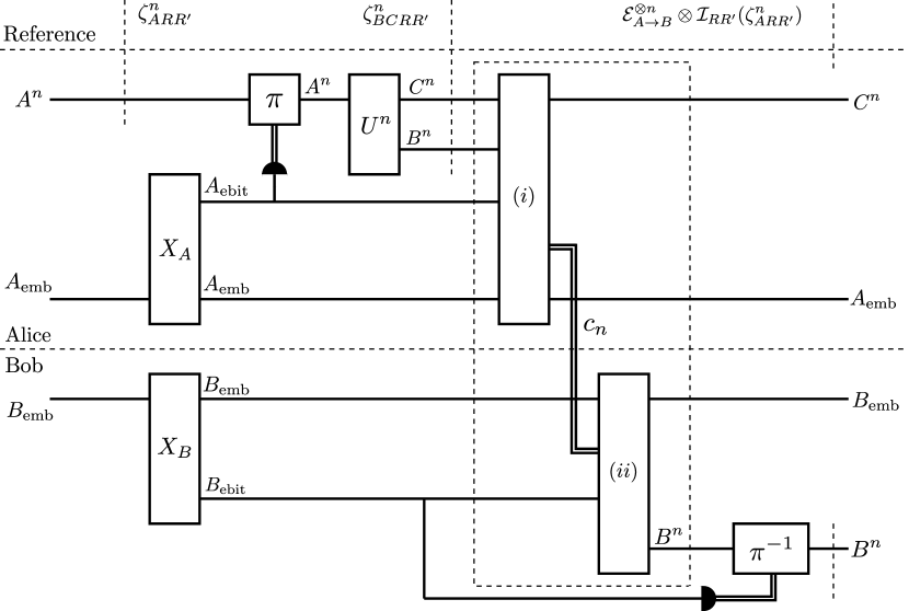
Figure 5.4: Circuit quantum reverse Shannon theorem.

A schematic description of the protocol that is used to prove the quantum reverse Shannon theorem. The channel simulation is done for the de Finetti type input state $\zeta^{n}_{ARR^{\prime}}$. Because our simulation is permutation invariant, the post-selection technique (Proposition LABEL:prop:postselect) shows that this is also sufficient for all input states. The whole simulation is called $\mathcal{P}^{n}$ in the text. (i) and (ii) denote the subroutine of quantum state splitting with embezzling states; with local operations on Alice’s and Bob’s side and a quantum communication rate of $q_{n}$.

Now we use this map as $\mathcal{P}^{n}_{A\rightarrow B}$ in (LABEL:eq:qrstpost). We obtain from the achievability of quantum state splitting with embezzling states (Theorem LABEL:thm:qssemb) that

$$P\left((\mathcal{E}_{A\rightarrow B}^{\otimes n}\otimes\mathcal{I}_{RR^{\prime}})(\zeta^{n}_{ARR^{\prime}}),(\mathcal{P}^{n}_{A\rightarrow B}\otimes\mathcal{I}_{RR^{\prime}})(\zeta^{n}_{ARR^{\prime}})\right)\leq\varepsilon+\varepsilon^{\prime}+\delta n\cdot\log|B|+|B|^{-n/2}\ ,$$ (5.68)

for a quantum communication cost

$$q_{n}\leq\frac{1}{2}\cdot I_{\max}^{\varepsilon^{\prime}}(B:RR^{\prime})_{(\mathcal{E}^{\otimes n}\otimes\mathcal{I})(\zeta^{n})}+2\log\frac{1}{\varepsilon}+4+\log n+\log\log|B|\ ,$$ (5.69)

where the last two terms on the right come from the fact that $\log\log|X_{B}|^{n}=\log n+\log\log|X_{B}|$. Because the trace distance is upper bounded by two times the purified distance (Lemma 2.3), this implies

$$\left\|\left((\mathcal{E}_{A\rightarrow B}^{\otimes n}-\mathcal{P}^{n}_{A\rightarrow B})\otimes\mathcal{I}_{RR^{\prime}})(\zeta^{n}_{ARR^{\prime}}\right)\right\|_{1}\leq 2(\varepsilon+\varepsilon^{\prime}+\delta n\cdot\log|B|+|B|^{-n/2})\ ,$$ (5.70)

and by choosing $\varepsilon=\varepsilon^{\prime}$, and $\delta=\frac{\varepsilon^{\prime}}{n\cdot\log|B|}$ we obtain

$$\|((\mathcal{E}_{A\rightarrow B}^{\otimes n}-\mathcal{P}^{n}_{A\rightarrow B})\otimes\mathcal{I}_{RR^{\prime}})(\zeta^{n}_{ARR^{\prime}})\|_{1}\leq 6\varepsilon^{\prime}+2\cdot|B|^{-n/2}\ .$$ (5.71)

Furthermore, we choose $\varepsilon^{\prime}=\frac{1}{6}\cdot\beta(n+1)^{-(|A|^{2}-1)}-\frac{1}{3}|B|^{-n/2}$ (for large enough $n$), and hence

$$\left\|\left((\mathcal{E}_{A\rightarrow B}^{\otimes n}-\mathcal{P}^{n}_{A\rightarrow B})\otimes\mathcal{I}_{RR^{\prime}})(\zeta^{n}_{ARR^{\prime}}\right)\right\|_{1}\leq\beta(n+1)^{-(|A|^{2}-1)}\ .$$ (5.72)

This is (LABEL:eq:qrstpost), and by the post-selection technique (Proposition LABEL:prop:postselect) this implies (LABEL:end).

It thus remains to show that the quantum communication rate of the resulting map is upper bounded by $Q_{E}$. Set

$$\chi=2\log\frac{1}{\varepsilon^{\prime}}+4+\log n+\log\log|B|\ ,$$ (5.73)

and it follows from (5.69) and below that the quantum communication cost of $\mathcal{P}^{n}_{A\rightarrow B}$ is quantified by

$$q_{n}\leq\frac{1}{2}\cdot I_{\max}^{\varepsilon^{\prime}}(B:RR^{\prime})_{(\mathcal{E}^{\otimes n}\otimes\mathcal{I})(\zeta^{n})}+\chi\ .$$ (5.74)

By the upper bound in Lemma LABEL:lem:maxdbound, and the fact that we can assume $|R^{\prime}|\leq(n+1)^{|A|^{2}-1}$ (Proposition LABEL:prop:postselect), we get

$$q_{n} \leq\frac{1}{2}\cdot I_{\max}^{\varepsilon^{\prime}}(B:R)_{(\mathcal{E}^{\otimes n}\otimes\mathcal{I})(\zeta^{n})}+\log|R^{\prime}|+\chi$$

$$\leq\frac{1}{2}\cdot I_{\max}^{\varepsilon^{\prime}}(B:R)_{(\mathcal{E}^{\otimes n}\otimes\mathcal{I})(\zeta^{n})}+\log\left((n+1)^{|A|^{2}-1}\right)+\chi\ .$$ (5.75)

By a corollary of Carathéodory’s theorem (Corollary LABEL:cor:cara), we can write

$$\zeta_{AR}^{n}=\sum_{i}p_{i}(\rho^{i}_{AR})^{\otimes n}\ ,$$ (5.76)

where $\rho^{i}_{AR}\in\mathcal{V}(\mathcal{H}_{AR})$, $i\in\{1,2,\ldots,(n+1)^{2|A||R|-2}\}$, and $\{p_{i}\}$ a probability distribution. Using a quasi-convexity property of the smooth max-information (Lemma LABEL:lem:imaxqconvex) we then obtain

$$q_{n} \leq\frac{1}{2}\cdot I_{\max}^{\varepsilon^{\prime}}(B:R)_{(\mathcal{E}^{\otimes n}\otimes\mathcal{I})(\sum_{i}p_{i}(\rho^{i})^{\otimes n})}+\log\left((n+1)^{|A|^{2}-1}\right)+\chi$$

$$\leq\frac{1}{2}\cdot\max_{i}I_{\max}^{\varepsilon^{\prime}}(B:R)_{\left[(\mathcal{E}\otimes\mathcal{I})(\rho^{i})\right]^{\otimes n}}+\log\left((n+1)^{|A||R|-1}\right)+\log\left((n+1)^{|A|^{2}-1}\right)+\chi$$

$$\leq\frac{1}{2}\cdot\max_{\rho}I_{\max}^{\varepsilon^{\prime}}(B:R)_{\left[(\mathcal{E}\otimes\mathcal{I})(\rho)\right]^{\otimes n}}+\log\left((n+1)^{|A||R|-1}\right)+\log\left((n+1)^{|A|^{2}-1}\right)+\chi\ ,$$ (5.77)

where the last maximum ranges over all $\rho_{AR}\in\mathcal{V}(\mathcal{H}_{AR})$. From the asymptotic equipartition property for the smooth max-information (Lemma LABEL:lem:aepimax) we obtain

$$q_{n}\leq \;n\cdot\frac{1}{2}\cdot\max_{\rho}I(B:R)_{(\mathcal{E}\otimes\mathcal{I})(\rho)}+\sqrt{n}\cdot\frac{\xi(\varepsilon^{\prime})}{2}-\log\frac{\varepsilon^{\prime 2}}{24}+\log\left((n+1)^{|A||R|-1}\right)$$

$$+\log\left((n+1)^{|A|^{2}-1}\right)+\chi\ ,$$ (5.78)

where $\xi(\varepsilon^{\prime})=8\cdot\sqrt{13-4\cdot\log\varepsilon^{\prime}}\cdot(2+\frac{1}{2}\cdot\log|A|)$. Since $\varepsilon^{\prime}=\frac{1}{6}\cdot\beta(n+1)^{-(|A|^{2}-1)}-\frac{1}{3}|B|^{-n/2}$, the quantum communication rate is then upper bounded by

$$q =\limsup_{\beta\rightarrow 0}\limsup_{n\rightarrow\infty}\frac{q_{n}}{n}\leq\frac{1}{2}\cdot\max_{\rho}I(B:R)_{(\mathcal{E}\otimes\mathcal{I})(\rho)}\ .$$ (5.79)

Thus it only remains to justify why it is sufficient that the maximally entangled states, which we used to make the protocol permutation invariant, only have finite precision. For this, it is useful to think of the channel $\mathcal{P}^{n}_{A\rightarrow B}$ that we constructed above, as in Figure LABEL:fig:emb (b). Let $\varepsilon^{\prime\prime}>0$ and assume that the entanglement is $\varepsilon^{\prime\prime}$-close to the perfect input state $\mu_{A_{\mathrm{emb}}B_{\mathrm{emb}}}\otimes\Phi^{m}_{A_{\mathrm{ebit}}B_{\mathrm{ebit}}}$. The purified distance is monotone (Lemma 2.4), and hence the corresponding imperfect output state is $\varepsilon^{\prime\prime}$-close to the state obtained under the assumption of perfect permutation invariance. Since $\varepsilon^{\prime\prime\prime}$ can be made arbitrarily small (Definition LABEL:def:emb), the channel based on the imperfect entanglement does the job. ∎

5.2.4 Discussion

Quantum Feedback Simulation.

Our main result (Theorem LABEL:thm:qrst) concerns the case of a non-feedback quantum channel simulation. But for the corresponding feedback version, we can just modify the Definitions LABEL:def:oneqrst and LABEL:def:qrstasym by exchanging the channel $\mathcal{E}_{A\rightarrow B}$ in (LABEL:eq:oneqrst) with its Stinespring dilation $U_{A\rightarrow BE}$ (where the register $E$ is at Alice’s side). It is then obvious from our proof strategy (e.g., this can be seen from (LABEL:eq:dilationidea)), that Theorem LABEL:thm:qrst also holds for the feedback case. Hence, we have the following corollary.

Corollary 5.10.

Let $\mathcal{E}_{A\rightarrow B}:\mathcal{B}(\mathcal{H}_{A})\rightarrow\mathcal{B}(\mathcal{H}_{B})$ be a channel. Then, the minimal quantum communication cost of asymptotic feedback reverse Shannon simulations for $\mathcal{E}_{A\rightarrow B}$ is equal to the entanglement assisted classical capacity of $\mathcal{E}_{A\rightarrow B}$.

Classical Communication.

The entanglement assisted classical capacity $C_{E}$ and the entanglement assisted quantum capacity $Q_{E}$ of quantum channels are equivalent by the means of quantum teleportation [Bennett93] and superdense coding [Bennett92]: $C_{E}=2\cdot Q_{E}$. By the same reasoning we also get the equivalence for the corresponding reverse capacities: $C_{\mathrm{QRST}}=2\cdot Q_{\mathrm{QRST}}$.

Without Embezzling States.

A natural follow up question is to ask for the rate trade-off between the different resources needed (classical communication, quantum communication, shared randomness, entanglement) to achieve channel simulations. We mention that some quantum channel simulation results with free entanglement in the form of maximally entangled states are discussed in [Bennett09]. A quantum communication rate of $Q_{E}$ is then not achievable, but additional communication is needed in order to deal with the problem of entanglement spread [Harrow09].

5.3 Universal Measurement Compression

The results in this section have been obtained in collaboration with Joseph Renes and Mark Wilde, and have appeared in [Berta13]. We show that quantum-classical channels, i.e., quantum measurements, can be simulated by an amount of classical communication equal to the quantum mutual information of the measurement, if sufficient shared randomness is available. Our result is a generalization of the classical reverse Shannon theorem to quantum-classical channels. In this sense, it is as a quantum reverse Shannon theorem for quantum-classical channels, but with the entanglement assistance and quantum communication replaced by shared randomness and classical communication, respectively. However, our result is also a generalization of Winter’s measurement compression theorem for fixed independent and identically distributed inputs [Winter04] to arbitrary inputs. In this spirit, we want to argue that our channel simulation result identifies the quantum mutual information of a quantum measurement as the information gained by performing it, independent of the input state on which it is performed.

5.3.1 Identifying the Information Gain of Quantum Measurements

Measurement is an integral part of quantum theory. It is the means by which we gather information about a quantum system. Although the classical notion of a measurement is rather straightforward, the quantum notion of measurement has been the subject of much thought and debate [Einstein49]. One interpretation is that the act of measurement on a quantum system causes it to abruptly jump or collapse into one of several possible states with some probability, an evolution seemingly different from the smooth, unitary transitions resulting from Schrödinger’s wave equation. Some have advocated for a measurement postulate in quantum theory [Dirac82], while others have advocated that our understanding of quantum measurement should follow from other postulates [Zurek09].

In spite of the aforementioned difficulties in understanding and interpreting quantum measurement, there is a precise question that one can formulate concerning it: how much information is gained by performing a given quantum measurement? This question has a rather long history, which to our knowledge begins with the work of Groenewold [Groenewold71]. In 1971, Groenewold argued on intuitive grounds for the following entropy reduction to quantify the information gained by performing a quantum measurement

$$H(\rho)-\sum_{x}p_{x}H(\rho_{x})\ ,$$ (5.80)

where $\rho$ is the initial state before the measurement occurs, and $\{p_{x},\rho_{x}\}$ is the post-measurement ensemble induced by the measurement. The intuition behind this measure is that it quantifies the reduction in uncertainty after performing a quantum measurement on a quantum system in state $\rho$, and its form is certainly reminiscent of a Holevo-like quantity [Holevo73], although the classical data in the above Groenewold quantity appears at the output of the process rather than at the input as in the case of the Holevo quantity. Groenewold left open the question of whether this quantity is non-negative for all measurements, and Lindblad proved that non-negativity holds whenever the measurement is of the von Neumann-Lüders kind (projecting onto an eigenspace of an observable) [Lindblad72]. Ozawa then settled the matter by proving that the above quantity is non-negative if and only if the post-measurement states are of the form

$$\rho_{x}=\frac{M_{x}\rho M_{x}^{\dagger}}{\operatorname{tr}[M_{x}^{\dagger}M_{x}\rho]}\ ,$$ (5.81)

for some operators $\{M_{x}\}$ such that $\sum_{x}M_{x}^{\dagger}M_{x}=\mathbbm{1}$ [Ozawa86]. Such measurements are termed efficient, and differ from general measurements as the latter may have several operators $M_{x,s}$ corresponding to the result $x$ [Fuchs01].

The fact that the quantity in (5.80) can become negative for some quantum measurements excludes it from being a generally appealing measure of information gain. To remedy this situation, Buscemi et al. later advocated for the following measure to characterize the information gain of a quantum measurement $\mathcal{M}$ when acting upon a particular state $\rho$ [Buscemi08, Luo10, Shirokov11, Wilde12_2],

$$I(X:R)_{(\mathcal{M}\otimes\mathcal{I})(\rho)}=H(X)_{\mathcal{M}(\rho)}+H(R)_{\rho}-H(XR)_{(\mathcal{M}\otimes\mathcal{I})(\rho)}\ ,$$ (5.82)

the quantum mutual information of the state

$$(\mathcal{M}\otimes\mathcal{I}_{R})(\rho_{AR})=\sum_{x}|x\rangle\langle x|_{X}\otimes\operatorname{tr}_{A}\big{[}(\mathcal{M}_{x}\otimes\mathcal{I}_{R})(\rho_{AR})\big{]}\ ,$$ (5.83)

where $\mathcal{M}=\{\mathcal{M}_{x}\}$, $X$ is a classical register containing the outcome of the measurement, and $\rho_{AR}$ is a purification of the initial state $\rho$ on system $A$ to a purifying system $R$. The advantages of the measure of information gain in (5.82) are as follows:

• It is non-negative.

• It reduces to Groenewold’s quantity in (5.80) for the special case of measurements of the form in (5.81) [Buscemi08].

• It characterizes the trade-off between information and disturbance in quantum measurements [Buscemi08].

• It has an operational interpretation in Winter’s measurement compression protocol as the optimal rate at which a measurement gathers information [Winter04].

This last advantage is the most compelling one from the perspective of quantum information theory; one cannot really justify a measure as an information measure unless it corresponds to a meaningful information processing task. Indeed, when reading the first few paragraphs of Groenewold’s paper [Groenewold71], it becomes evident that his original motivation was information theoretic in nature, and with this in mind, Winter’s measure in (5.82) is clearly the one Groenewold was seeking after all.

In spite of the above arguments in favor of the information measure in (5.82) as a measure of information gain, it is still lacking in one aspect: it is dependent on the state on which the quantum measurement $\mathcal{M}$ acts in addition to the measurement itself. A final requirement that one should impose for a measure of information gain by a measurement is that it should depend only on the measurement itself. A simple way to remedy this problem is to maximize the quantity in (5.82) over all possible input states, leading to the following characterization of information gain

$$I(\mathcal{M})=\max_{\rho}I(X:R)_{(\mathcal{M}\otimes\mathcal{I})(\rho)}\ ,$$ (5.84)

for $(\mathcal{M}\otimes\mathcal{I}_{R})(\rho_{AR})$ as in (5.83). The quantity above has already been identified and studied by previous authors as an important information quantity, being labeled as the purification capacity of a measurement [Jacobs03, Jacobs06] or the information capacity of a quantum observable [Holevo12]. The above quantity also admits an operational interpretation as the entanglement-assisted capacity of a quantum measurement for transmitting classical information [Bennett02, Bennett99, Holevo02, Holevo12], though it is our opinion that this particular operational interpretation is not sufficiently compelling such that we should associate the measure in (5.84) with the notion of information gain. Here, the aim is to address this issue by providing a compelling operational interpretation of the measure in (5.84), and our contribution is to show that $I(\mathcal{M})$ is the optimal rate at which a measurement gains information when many identical instances of it act on an arbitrary input state.

In more detail, let $\mathcal{H}_{A}$ denote the input for a given measurement $\mathcal{M}$. We suppose that a third party prepares an arbitrary quantum state on $\mathcal{H}_{A}^{\otimes n}$, where $n$ is a large positive number. A sender and receiver can then exploit some amount of shared random bits and classical communication to simulate the action of $n$ instances of the measurement $\mathcal{M}$ (denoted by $\mathcal{M}^{\otimes n}$) on the chosen input state, in such a way that it becomes physically impossible for the third party, to whom the receiver passes along the measurement outcomes, to distinguish between the simulation and the ideal measurement $\mathcal{M}^{\otimes n}$ as $n$ becomes large (the third party can even keep the purifying system of a purification of the chosen input state in order to help the distinguishing task). This information-theoretic task is known as channel simulation (depicted in Figure 5.5). By design, the information gained by the measurement is that relayed by the classical communication. Following [Winter04], we call this task universal measurement compression. We prove that the optimal rate of classical communication is equal to $I(\mathcal{M})$, if sufficient shared randomness is available. In our opinion, this result establishes (5.84) as the information-theoretic measure of information gain of a quantum measurement.

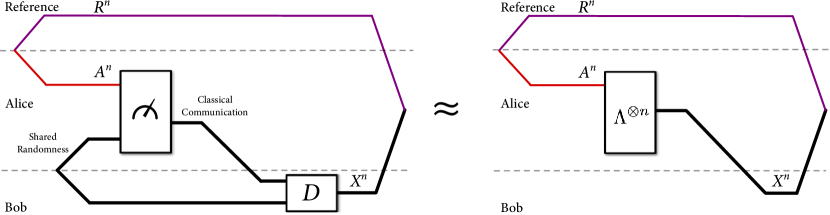
Figure 5.5: Universal measurement compression.

Simulation (left) of the measurement $\Lambda^{\otimes n}$ (right). In the simulation, Alice uses shared randomness to perform a new measurement, whose result she communicates to Bob, such that Bob can recover the actual measurement output $X^{n}$ using the message and the shared randomness. If the simulation scheme works for any input, we can associate the amount of communication with the information gained by the measurement.

We also characterize the optimal rate region consisting of the rates of shared randomness and classical communication that are both necessary and sufficient for the existence of a measurement simulation, for the feedback and the non-feedback case. Note that if sufficient shared randomness is available, and we are only interested in quantifying the rate of classical communication, then there is no advantage of a non-feedback simulation over a feedback one, the optimal rate of classical communication is given by (5.84).

5.3.2 Proof Ideas

The proof technique is the same as in our proofs of the classical and quantum reverse Shannon theorems (Sections LABEL:se:shannon and LABEL:se:qshannon). In fact, we can think of our approach here as a classicalized or dephased version of our proof of the quantum reverse Shannon theorem. In particular, the proof is also based on one-shot information theory and uses the smooth entropy formalism. In addition, we make use of the idea of classically coherent states. We say that a pure state $|{\psi}\rangle\!\langle{\psi}|_{X_{A}X_{B}R}\in\mathcal{V}(\mathcal{H}_{X_{A}X_{B}R})$ is classically coherent with respect to systems $X_{A}X_{B}$ if there is an orthonormal basis $\{|{x}\rangle\}$ such that $|{\psi}\rangle$ can be written in the form

$$|{\psi}\rangle_{X_{A}X_{B}R}=\sum_{x}\sqrt{p_{x}}\,|{xx}\rangle_{X_{A}X_{B}}\otimes|{\psi_{x}}\rangle_{R}\ ,$$ (5.85)

for some probability distribution $\{p_{x}\}$, and pure states $|{\psi_{x}}\rangle\!\langle{\psi_{x}}|_{R}\in\mathcal{V}(\mathcal{H}_{R})$. Harrow realized the importance of classically coherent states for quantum communication tasks [Harrow04], while [Dupuis12, Szehr11] recently exploited this notion in devising a decoupling approach to the Holevo-Schumacher-Westmoreland coding theorem [Holevo98, Schumacher97] that is useful for our purposes here.

We begin by establishing a protocol known as classically coherent state merging, which is a variation of the well-known state merging protocol [Horodecki05, Horodecki07] specialized to classically coherent states. For the analysis we require a strong classical min-entropy randomness extractor against quantum side information (as discussed in Section LABEL:se:cc). We then show how time-reversing this protocol and exchanging the roles of Alice and Bob leads to a protocol known as classically coherent state splitting. It suffices for our purposes for this protocol to use shared randomness and classical communication rather than entanglement and quantum communication, respectively. Generalizing this last protocol then leads to a one-shot channel simulation which is essentially optimal when acting on a single copy of a known state. Finally, we exploit the post-selection technique for quantum channels (see Appendix LABEL:ap:postselect), and the aforementioned state splitting protocol to show that it suffices to simulate many instances of a measurement on a purification of a particular de Finetti quantum input state in order to guarantee that the simulation is asymptotically perfect when acting on an arbitrary quantum state. For the non-feedback case we additionally need the idea of randomness recycling [Bennett09].

5.3.3 Classically Coherent State Merging and State Splitting

We first establish one-shot protocols for state merging and state splitting of classically coherent quantum states. The main technical ingredient for the construction of these protocols are permutation based strong classical min-entropy extractors against quantum side information. Since we only care about the optimal output size of the extractor and not about its seed size, we will just use a family of pairwise independent permutations. Proposition LABEL:prop:ccperm about the extractor properties of families of pairwise independent permutations can then be rephrased as follows.

Corollary 5.11.

Let $\varepsilon>0$, $\rho_{XR}\in\mathcal{S}_{\leq}(\mathcal{H}_{XR})$ be classical on $X$ with respect to a basis $\{|{x}\rangle\}_{x\in X}$, and $\{P_{X}^{j}\}_{j\in J}$ be a family of pairwise independent permutations. Furthermore, consider a decomposition of the system $X$ into two subsystems $X_{1}$ and $X_{2}$, and define

$$\sigma_{X_{1}R}^{j}=\operatorname{tr}_{X_{2}}\left[(P_{X}^{j}\otimes\mathbbm{1}_{R})\rho_{XR}(P_{X}^{j}\otimes\mathbbm{1}_{R})^{\dagger}\right]\ .$$ (5.86)

If we choose

$$\log|X_{1}|\leq H_{\min}(X|R)_{\rho}-2\log\frac{1}{\varepsilon}\ ,$$ (5.87)

then we have that

$$\frac{1}{|J|}\cdot\sum_{j\in J}\left\|\sigma_{X_{1}R}^{j}-\frac{\mathbbm{1}_{X_{1}}}{|X_{1}|}\otimes\rho_{R}\right\|_{1}\leq\varepsilon\ .$$ (5.88)

We mention that classical randomness extractors against quantum side information already proved useful in quantum coding theory [Dupuis12].

Definition 5.7 (State Merging for classically coherent states).

Consider a bipartite system with parties Alice and Bob. Let $\varepsilon>0$, and $\rho_{X_{A}X_{B}BR}\in\mathcal{V}_{\leq}(\mathcal{H}_{X_{A}X_{B}BR})$ be classically coherent on $X_{A}X_{B}$ with respect to the basis $\{|{x}\rangle\}_{x\in X_{A}X_{B}}$, where Alice controls $X_{A}$, Bob $X_{B}B$, and $R$ is a reference system. A quantum protocol $\mathcal{E}$ is called an $\varepsilon$-error state merging of $\rho_{X_{A}X_{B}BR}$ if it consists of applying local operations at Alice’s side, sending $q$ qubits from Alice to Bob, local operations at Bob’s side, and it outputs a state $\omega_{X_{B^{\prime}}X_{B}BRX_{A_{1}}B_{1}}=(\mathcal{E}\otimes\mathcal{I}_{R})(\rho_{X_{A}X_{B}BR})$ such that

$$\omega_{X_{B^{\prime}}X_{B}BRX_{A_{1}}B_{1}}\approx_{\varepsilon}\mathcal{I}_{X_{A}\rightarrow X_{B^{\prime}}}(\rho_{X_{A}X_{B}BR})\otimes\Phi^{E}_{X_{A_{1}}B_{1}}\ ,$$ (5.89)

where $\Phi^{E}_{X_{A_{1}}B_{1}}$ is a maximally entangled state of Schmidt rank $E$. The quantity $q$ is called quantum communication cost, and $e=\lfloor\log E\rfloor$ entanglement gain.

Lemma 5.12.

Let $\varepsilon>0$, and $\rho_{X_{A}X_{B}BR}\in\mathcal{V}_{\leq}(\mathcal{H}_{X_{A}X_{B}BR})$ be classically coherent on $X_{A}X_{B}$ with respect to the basis $\{|{x}\rangle\}_{x\in X_{A}X_{B}}$. Then, there exists an $\varepsilon$-error state merging protocol for $\rho_{X_{A}X_{B}BR}$ with quantum communication cost

$$q=\left\lceil H_{0}(X_{A})_{\rho}-H_{\min}(X_{A}|R)_{\rho}+4\log\frac{1}{\varepsilon}\right\rceil\ ,$$ (5.90)

and entanglement gain

$$e=\left\lfloor H_{\min}(X_{A}|R)_{\rho}-4\log\frac{1}{\varepsilon}\right\rfloor\ .$$ (5.91)

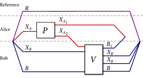
Figure 5.6: State merging of classically coherent states.

The protocol from the proof of Lemma 5.12 for state merging of a classically coherent state on systems $RX_{A}X_{B}B$. The operation $P$ is a permutation of states in the orthonormal basis $\{|{x}\rangle\}$ of $X_{A}$, and it also splits $X_{A}$ into two subsystems. The operation $V$ is an isometry guaranteed by Uhlmann’s theorem to complete the merging task, while also generating entanglement between Alice and Bob.