Standard finite elements for the numerical resolution of the elliptic Monge-Ampère equation: classical solutions

Abstract.

We propose a new variational formulation of the elliptic Monge-Ampère equation and show how classical Lagrange elements can be used for the numerical resolution of classical solutions of the equation. Error estimates are given for Lagrange elements of degree $d\geq 2$ in dimensions 2 and 3. No jump term is used in the variational formulation. We propose to solve the discrete nonlinear system of equations by a time marching method and numerical evidence is given which indicates that one approximates weak solutions in two dimensions.

1. Introduction

This paper addresses the numerical resolution of the Dirichlet problem for the Monge-Ampère equation

(1.1) $$\det D^{2}u=f\ \text{in}\ \Omega,\quad u=g\ \text{on}\ \partial\Omega.$$

A classical solution of (1.1) is a convex function $u\in C(\overline{\Omega})\cap C^{2}(\Omega)$ which satisfies (1.1). The domain $\Omega\subset\mathbb{R}^{n},n=2,3$ is assumed to be convex with (polygonal) boundary $\partial\Omega$. Here $D^{2}u=\bigg{(}\frac{\partial^{2}u}{\partial x_{i}\partial x_{j}}\bigg{)}_{i,j=1,\ldots,n}$ is the Hessian of $u$ and $f,g$ are given functions with $f\geq 0$ and $g\in C(\partial\Omega)$ with $g$ convex on any line segment in $\partial\Omega$. A smooth solution of (1.1) solves the variational problem: find $u\in W^{2,\infty}(\Omega)$ such that $u=g\ \text{on}\ \partial\Omega$ and

$$\int_{\Omega}(\det D^{2}u)v\,dx=\int_{\Omega}fv\,dx,\,\text{for all}\,v\in H^{1}_{0}(\Omega).$$

We propose to solve numerically (1.1) with standard Lagrange finite element spaces $V_{h}$ of degree $d\geq 2$ by analyzing the (nonconforming) variational problem: find $u_{h}\in V_{h}\subset H^{1}(\Omega)$ such that $u_{h}=g_{h}\ \text{on}\ \partial\Omega$ for an interpolant $g_{h}$ of $g$ and

(1.2) $$\sum_{K\in\mathcal{T}_{h}}\int_{K}(\det D^{2}u_{h})v_{h}\,dx=\int_{\Omega}fv_{h}\,dx,\forall v_{h}\in V_{h}\cap H^{1}_{0}(\Omega).$$

Here $\mathcal{T}_{h}$ denotes a quasi-uniform, simplicial and conforming triangulation of the domain. Error estimates for smooth solutions are derived. We propose to solve the discrete nonlinear system of equations by a time marching method, c.f. Theorem 3.3. Numerical evidence is given which indicates that one approximates weak solutions in two dimensions.

Closely related to this paper are [6, 5, 13]. Like the authors of these papers, we also use a fixed point argument but our approach is essentially different. No jump term is used in our variational formulation. We are able to give error estimates for Lagrange elements of degree $d\geq 2$ with no smoothness assumption on the boundary. This is achieved by a rescaling argument. The fixed point argument we use to establish the well-posedness of (1.2) also yields the theoretical convergence of the time marching iterative method.

The use of the standard Lagrange finite element spaces in connection with the numerical resolution of (1.1) also appears in mixed methods. A least squares formulation was used in [10] and recently a direct mixed formulation was presented in [12]. The latter is essentially the limiting case of the mixed method for the vanishing moment methodology, c.f. [9] and the references therein. The vanishing moment methodology is a singular perturbation approach to the Monge-Ampère equation with the perturbation a multiple of the bilaplacian. The convergence and error estimates for the methods introduced in [10] are still open problems and mixed methods typically lead to large system of equations.

In view of having numerical results for non smooth solutions, it is natural to use a time marching method, and not Newton’s method, for solving the discrete nonlinear system of equations. The numerical experiments indicate that the method may be valid for the so-called viscosity solutions. This is a fascinating and challenging issue and its resolution involves additional new ideas different from the techniques for error analysis used in this paper. We wish to address this issue in a separate work [4].

Our approach may be viewed as a variant of the method introduced in [5]. As pointed out in [5] a numerical method based on Lagrange elements and the formulation (1.2) does not work in theory in the sense it is difficult to use a fixed point argument which consists in linearization at the exact solution. The authors in [5] ingeniously added jump terms to facilitate the above approach. On the other hand, our numerical experiments indicate that the above approach works if the discrete nonlinear system of equations is solved by a time marching method. An advantage of the time marching method is that the user only needs access to a Poisson solver to implement the scheme. The main advantage however is that one has numerical evidence of convergence for non-smooth solutions. Obviously the time marching method can also be applied to the discretization proposed in [5] but we believe that in the context of non-smooth solutions the jump terms in the discretization proposed there may not be necessary. We have chosen not to treat curved boundaries for simplicity and to focus on the main ideas. The main motivation to assume that the domain is smooth and strictly convex is to guarantee the existence of a smooth solution for smooth data. One then faces the difficulty of practically imposing Dirichlet boundary conditions, a problem solved in [5] by the use of Nitsche method. Here instead we will make the assumption ubiquitous in finite element analysis of numerous problems that the solution is smooth on a polygonal domain.

We believe that the fixed point argument used in this paper and/or the strategy of rescaling the Monge-Ampère equation would prove useful in resolving other outstanding issues about the numerical analysis of Monge-Ampère type equations, see for example [3]. For another example, our fixed point-rescaling argument provides an alternative to [13] for the proof of the well-posedness of the discretization proposed in [5, 6] for quadratic finite elements. Essentially, the rescaling argument is appropriate whenever an argument can be made that a result holds for the Monge-Ampère equation provided the solution is sufficiently small. Thus, instead of describing the whole rescaling argument, one may simply prove results for the case when the exact solution is sufficiently small.

In fact the results of this paper are similar to the ones announced in the context of $C^{1}$ conforming approximations in a technical report by the author [1] but the analysis is more involved. Exploiting that similarity, pseudo transient continuation methods can be developed for (1.1) by taking appropriate nonconforming discretizations of the iterative methods proposed in [1]. We do not pursue this line of investigation in this paper. The properties of the Lagrange finite element spaces used in our analysis, namely an approximation property and inverse estimates, also hold for certain $C^{1}$ conforming approximations. Thus our error estimates hold for these as well. The error estimates hold for weaker assumptions on the exact solution, namely that $u\in W^{3,\infty}(K)$ on each element $K$, is strictly convex on each element and solves (1.2).

We organize the paper as follows. In section 2, we give the notation used and recall some facts about determinants and Lagrange finite element spaces. The properties of the finite element spaces needed for our analysis are stated as well as the requirements on the exact solution. We prove existence and uniqueness of the discrete problem (1.2) with the convergence of the time marching method in section 3. In section 4 we give the numerical results.

2. Notation and Preliminaries

Let $\mathbb{P}_{d}$ denote the space of polynomials of degree less than or equal to $d$. We use the usual notation $L^{p}(\Omega),2\leq p\leq\infty$ for the Lebesgue spaces and $W^{s,p}(\Omega),1\leq s<\infty$ for the Sobolev spaces of elements of $L^{p}(\Omega)$ with weak derivatives of order less than or equal to $s$ in $L^{p}(\Omega)$. The norms and semi-norms in $W^{s,p}(\Omega)$ are denoted by $||\,||_{s,p}$ and $|\,|_{s,p}$ respectively and when $p=2$ we will simply use $||\,||_{s}$ and $|\,|_{s}$. Thus the $L^{p}$ norm is denoted $||\,||_{0}$. We will use the simpler notation $||\ ||_{\infty}$ for the norm in $L^{\infty}(\Omega)$.

For a function defined on an element $K$ or more generally on a subdomain $S$, we will add $K$ or $S$ to the norm and semi-norm notation. We will need a broken Sobolev norm

$$||v||_{s,p,\mathcal{T}_{h}}=\bigg{(}\sum_{K\in\mathcal{T}_{h}}||v||_{s,p,K}^{p}\bigg{)}^{\frac{1}{p}},$$

with the above conventions for the case when $p=2$.

For a matrix field $A$, we define $||A||_{\infty}=\max_{i,j=1,\ldots n}||A_{ij}||_{\infty}$. We denote by $n$ the unit outward normal vector to $\partial\Omega$ and by $n_{K}$ the unit outward normal vector to $\partial K$ for an element $K$.

For two matrices $A=(A_{ij})$ and $B=(B_{ij})$, $A:B=\sum_{i,j=1}^{n}A_{ij}B_{ij}$ denotes their Frobenius inner product. The divergence of a matrix field is understood as the vector obtained by taking the divergence of each row. We use the notation $Du$ to denote the gradient vector and for a matrix $A$, $\operatorname{cof}A$ denotes the matrix of cofactors of $A$.

A quantity which is constant is simply denoted by $C$. Throughout the paper, for a discrete function $v_{h}$, the Hessian $D^{2}v_{h}$ is always computed element by element. We will assume that $0<h\leq 1$.

2.1. Computations with determinants

Lemma 2.1.

For $u,v\in C^{2}(K)$ we have

$$\det D^{2}u-\det D^{2}v=\operatorname{cof}(tD^{2}u+(1-t)D^{2}v):(D^{2}u-D^{2}v),$$

for some $t\in[0,1]$.

Proof.

The result follows from the mean value theorem and the expression of the derivative of the mapping $F:u\to\det D^{2}u$. We have $F^{\prime}(u)(v)=(\operatorname{cof}D^{2}u):D^{2}v$. First note that $\partial(\det A)/(\partial A_{ij})=(\operatorname{cof}A)_{ij}$. See for example formula (23) p. 440 of [8]. The result then follows from the chain rule. ∎

Lemma 2.2.

For $n=2$ and $n=3$, and two matrix fields $\eta$ and $\tau$

(2.1) $$||\operatorname{cof}(\eta):\tau||_{0} \leq C||\eta||_{\infty}^{n-1}||\tau||_{0}$$

(2.2) $$||\operatorname{cof}(\eta)-\operatorname{cof}(\tau)||_{0} \leq C(||t\eta+(1-t)\tau||_{\infty})^{n-2}||\eta-\tau||_{0}.$$

Proof.

The bound (2.1) is given by a direct computation. For $n=2$, we have $\operatorname{cof}(\eta)-\operatorname{cof}(\tau)=\operatorname{cof}(\eta-\tau)$ from which the result follows. For $n=3$ we use the mean value theorem. It is enough to estimate the first entry of $\operatorname{cof}(\eta)-\operatorname{cof}(\tau)$ which is equal to

$$\det\begin{pmatrix}\eta_{22}&\eta_{23}\\ \eta_{32}&\eta_{33}\end{pmatrix}-\det\begin{pmatrix}\tau_{22}&\tau_{23}\\ \tau_{32}&\tau_{33}\end{pmatrix} =\operatorname{cof}\bigg{(}t\begin{pmatrix}\eta_{22}&\eta_{23}\\ \eta_{32}&\eta_{33}\end{pmatrix}+(1-t)\begin{pmatrix}\tau_{22}&\tau_{23}\\ \tau_{32}&\tau_{33}\end{pmatrix}\bigg{)}:$$

$$\begin{pmatrix}\eta_{22}-\tau_{22}&\eta_{23}-\tau_{23}\\ \eta_{32}-\tau_{32}&\eta_{33}-\tau_{33}\end{pmatrix},$$

for some $t\in[0,1]$. Direct computation then give (2.2). ∎

2.2. Assumptions on the approximation spaces

For the discretization (1.2), one can use either the Lagrange finite element spaces or certain finite dimensional spaces of $C^{1}$ functions. To make our results applicable to other types of discretizations, we formulate our assumptions on the approximation spaces.

Assumption 2.3.

Approximation property. The finite dimensional space $V_{h}\subset H^{1}(\Omega)$ contains the Lagrange space of degree $d$

$$\{\,v_{h}\in C^{0}(\overline{\Omega}),v_{h}|_{K}\in\mathbb{P}_{d},\forall K\in\mathcal{T}_{h}\,\},$$

and there exists a linear interpolation operator $I_{h}$ mapping $C^{r}(\overline{\Omega})$ for $r=0$ or $r=1$ into $V_{h}$ and a constant $C$ such that if $w$ is in the Sobolev space $W^{l+1,p}(\Omega),1\leq p\leq\infty$, $0\leq l\leq d$

(2.3) $$||w-I_{h}w||_{k,p,\mathcal{T}_{h}}\leq C_{ap}h^{l+1-k}|w|_{l+1,p},$$

for $k=0,1,2$.

The interpolant $g_{h}$ used in (1.2) is taken as $I_{h}$ applied to a continuous extension of $g$.

When $V_{h}$ is the Lagrange finite element space, the interpolant $I_{h}$ is taken as the standard interpolation operator defined from the degrees of freedom. It is then known that Assumption 2.3 holds [7].

As a consequence of (2.3),

(2.4) $$||I_{h}w||_{k,p,\mathcal{T}_{h}}\leq(1+C_{ap})||w||_{k,p},w\in W^{k,p}(\Omega),k=0,1,2,$$

for all $p$.

Assumption 2.4.

Inverse estimates

(2.5) $$||w_{h}||_{t,p,\mathcal{T}_{h}}\leq C_{inv}h^{s-t+\min(0,\frac{n}{p}-\frac{n}{q})}||w_{h}||_{s,q,\mathcal{T}_{h}},$$

for $0\leq s\leq t,1\leq p,q\leq\infty$ and $w_{h}\in V_{h}$.

The inverse estimates hold for the Lagrange finite element spaces as a consequence of the quasi-uniformity assumption on the triangulation [7].

2.3. Assumptions on the exact solution

Let $\lambda_{1}(A)$ and $\lambda_{n}(A)$ denote the smallest and largest eigenvalues of a symmetric matrix $A$. We make the following assumption on the exact solution:

Assumption 2.5.

Local piecewise smooth and strict convexity assumption. The solution $u$ of (1.1) is in $W^{3,\infty}(\mathcal{T}_{h})\cap H^{1}(\Omega)$, strictly convex on each element $T$ and for constants $m^{\prime},M^{\prime}>0$, independent of $h$

$$m^{\prime}\leq\lambda_{1}(D^{2}u(x))\leq\lambda_{n}(D^{2}u(x))\leq M^{\prime},\forall x\in K,K\in\mathcal{T}_{h}.$$

Moreover, we require the exact solution $u$ to solve the problem: find $u\in W^{2,\infty}(\mathcal{T}_{h})$, strictly convex on each element $T$, such that $u=g\ \text{on}\ \partial\Omega$ and

(2.6) $$\sum_{K\in\mathcal{T}_{h}}\int_{K}(\det D^{2}u)v\,dx=\int_{\Omega}fv\,dx,\forall v\in V_{h}\cap H^{1}_{0}(\Omega).$$

We note that Assumption 2.5 trivially holds for a strictly convex solution $u$ in $C^{3}(\overline{\Omega})$. In that case $f\geq c_{0}>0$ for a constant $c_{0}$. The main motivation of Assumption 2.5 is our claim in [4] that the numerical approximation of the viscosity solution of (1.1) can be reduced to solving problems of this type.

3. Well-posedness of the discrete problem and error estimates

The proof of all lemmas in this section are given at the end of the section.

We first state a fundamental observation about the behavior of discrete functions near the interpolant $I_{h}u$.

Lemma 3.1.

There exists $\delta>0$ such that for $h$ sufficiently small and for all $v_{h}\in V_{h}$ with $||v_{h}-I_{h}u||_{1}<\delta/(2C_{inv})h^{1+n/2}$, $D^{2}(v_{h}|_{K})$ is positive definite with

$$\frac{m^{\prime}}{2}\leq\lambda_{1}D^{2}(v_{h}|_{K})\leq\lambda_{n}D^{2}(v_{h}|_{K})\leq\frac{3M^{\prime}}{2}$$

where $m^{\prime}$ and $M^{\prime}$ are the constants of Assumption 2.5. Thus $\operatorname{cof}D^{2}(v_{h}|_{K})$ is invertible on each element $T$.

Let

(3.1) $$\delta_{h}=\frac{\delta}{2C_{inv}}h^{1+\frac{n}{2}}.$$

By Lemma 3.1, for $v_{h}\in V_{h},||v_{h}-I_{h}u||_{1}\leq\delta_{h}$, $v_{h}$ is piecewise strictly convex with smallest eigenvalue bounded below by $m^{\prime}/2$ and above by $3M^{\prime}/2$. Put

$$X_{h}=\{\,v_{h}\in V_{h},v_{h}=g_{h}\,\text{on}\,\partial\Omega,||v_{h}-I_{h}u||_{1}<\delta_{h}\,\}.$$

As a consequence of Assumption 2.5

Lemma 3.2.

There exists constants $m,M>0$ independent of $h$ such that for all $v_{h}\in X_{h}$

$$m\leq\lambda_{1}(\operatorname{cof}D^{2}v_{h}(x))\leq\lambda_{n}(\operatorname{cof}D^{2}v_{h}(x))\leq M,\forall x\in K,K\in\mathcal{T}_{h}.$$

It follows that

(3.2) $$m|w|_{1,K}^{2}\leq\int_{K}[(\operatorname{cof}\,D^{2}v_{h}(x))Dw(x)]\cdot Dw(x)\,\,dx\leq M|w|_{1,K}^{2},w\in H^{1}(K).$$

The main result of this section is the following theorem

Theorem 3.3.

Let the finite dimensional spaces $V_{h}\subset H^{1}(\Omega)$ contain piecewise polynomials of degree $d\geq 2$. Assume that the spaces $V_{h}$ satisfy Assumption 2.3 of approximation property and Assumption 2.5 of inverse estimates. Assume also that the exact solution $u\in W^{l+1,\infty}(\mathcal{T}_{h})\cap H^{1}(\Omega),2\leq l\leq d$ satisfies Assumption 2.5 of strict convexity and solves (2.6). Then the problem (1.2) has a unique solution $u_{h}$ which is strictly convex on each element and we have the error estimates

$$||u-u_{h}||_{2,\mathcal{T}_{h}} \leq Ch^{l-1}$$

$$||u-u_{h}||_{1} \leq Ch^{l},$$

for $h$ sufficiently small. Moreover, with a sufficiently close initial guess $u_{h}^{0}$, the sequence defined by, $u_{h}^{k+1}=g_{h}$ on $\partial\Omega$

(3.3) $$\begin{split}\frac{\nu}{\alpha^{n-1}}\int_{\Omega}Du_{h}^{k+1}\cdot Dv_{h}\,dx&=\frac{\nu}{\alpha^{n-1}}\int_{\Omega}Du_{h}^{k}\cdot Dv_{h}\,dx-\int_{\Omega}fv_{h}\,dx\\ &\quad\qquad\qquad\qquad+\sum_{K\in\mathcal{T}_{h}}\int_{K}(\det D^{2}u_{h}^{k})v_{h}\,dx,\end{split}$$

$\forall v_{h}\in V_{h}\cap H_{0}^{1}(\Omega)$, converges linearly to $u_{h}$ in the $H^{1}$ norm for $\nu=(M+m)/2,\alpha=h^{3}$ and for $h$ sufficiently small.

Before we give the proof of the above theorem we will state several lemmas whose proof are given at the end of the section.

We recall that $\alpha>0$ is a small parameter which may depend on $h$. For $\rho>0$, let

$$B_{h}(\rho)=\{v_{h}\in V_{h},v_{h}=g_{h}\,\text{on}\,\partial\Omega,||v_{h}-I_{h}u||_{1}\leq\rho\},$$

where we do not indicate the dependence of $B_{h}(\rho)$ on $\alpha$ for simplicity. The ball $B_{h}(\rho)$ is nonempty as it contains $I_{h}u$.

If $v_{h}\in B_{h}(\rho),||\alpha v_{h}-\alpha I_{h}u||_{1}\leq\alpha\rho$. Thus

(3.4) $$\alpha B_{h}(\rho)\subset X_{h}\,\text{for}\,\alpha\rho\leq\frac{\delta_{h}}{2}\,\text{which holds for }\,\alpha=h^{3}\,\text{and}\,h\,\text{small enough}.$$

For a given $v_{h}\in V_{h}$, $v_{h}=g_{h}$ on $\partial\Omega$, define $T(\alpha v_{h})\in V_{h}$ as the solution of

(3.5) $$\begin{split}\nu\int_{\Omega}DT(\alpha v_{h})\cdot Dw_{h}\,dx&=\nu\int_{\Omega}D(\alpha v_{h})\cdot Dw_{h}\,dx\\ &\qquad+\alpha^{n}\sum_{K\in\mathcal{T}_{h}}\int_{K}(\det D^{2}v_{h})w_{h}\,dx\\ &\qquad\qquad-\alpha^{n}\int_{\Omega}fw_{h}\,dx,\forall w_{h}\in V_{h}\cap H_{0}^{1}(\Omega),\end{split}$$

with $\alpha v_{h}-T(\alpha v_{h})=0$ on $\partial\Omega$ and we recall that $\nu=(M+m)/2$ where $M$ and $m$ are the constants of Lemma 3.2.

We will show that $T$ has a unique fixed point $\alpha u_{h}$ with $u_{h}$ in $B_{h}(\rho)$ for $h$ sufficiently small.

The motivation to introduce the damping parameter $\alpha$ is that it allows to solve a rescaled version of (1.1). Indeed $\det D^{2}u=f$ is equivalent to $\det\alpha D^{2}u=\alpha^{n}f$. Taking $\alpha$ as a power of $h$ will play a crucial role in proving the well-posedness of (1.2) and obtaining optimal error estimates.

Lemma 3.4.

The mapping $T$ is well defined and if $\alpha u_{h}$ is a fixed point of $T$, i.e. $T(\alpha u_{h})=\alpha u_{h}$, then $u_{h}$ solves (1.2).

The next lemma says that the mapping $T$ does not move the center $I_{h}u$ of a ball $B_{h}(\rho)$ too far.

Lemma 3.5.

We have

(3.6) $$||\alpha I_{h}u-T(\alpha I_{h}u)||_{1}\leq C_{1}\alpha^{n}h^{l-1}||u||_{2,\infty}^{n-1}||u||_{l+1},$$

The next two lemmas establish the contraction mapping property of $T$ under the assumption that $d\geq 2$ and $\alpha=h^{3}$.

Lemma 3.6.

For $h$ sufficiently small, and $\rho>0$, $T$ is a strict contraction mapping in the ball $\alpha B_{h}(\rho)$,i.e. for $v_{h},w_{h}\in B_{h}(\rho)$

$$||T(\alpha v_{h})-T(\alpha w_{h})||_{1}\leq a||\alpha v_{h}-\alpha w_{h}||_{1},0<a<1.$$

Lemma 3.7.

For $h$ sufficiently small and $\rho=1/(1-a)C_{1}\alpha^{n-1}h^{l-1}||u||_{l+1,\infty}^{n}$ where $C_{1}$ is the constant in Lemma 3.5, $T$ is a strict contraction in $\alpha B_{h}(\rho)$ and maps $\alpha B_{h}(\rho)$ into itself.

The previous lemmas will readily allows us to conclude the solvability of (1.2) and derive error estimates in the $H^{1}$ norm by using the explicit expression of the radius $\rho$ of the above lemma. We can now give the proof of Theorem 3.3.

Proof of Theorem 3.3.

Since the mapping $T$ is a strict contraction which maps $\alpha B_{h}(\rho)$ into itself, the existence of a fixed point $\alpha u_{h}$ with $u_{h}\in B_{h}(\rho)$ follows from the Banach fixed point theorem. By Lemma 3.4 $u_{h}$ solves (1.2).

From the expression of $\rho$ given in Lemma 3.7 we get using the value of $\alpha=h^{3}$

$$||u-u_{h}||_{1} \leq||u-I_{h}u||_{1}+||I_{h}u-u_{h}||_{1}\leq Ch^{l}|u|_{l+1}+2C_{1}\alpha^{n-1}h^{l-1}||u||_{2,\infty}^{n-1}||u||_{l+1}$$

$$\leq Ch^{l}+2C_{1}h^{l+3n-4}||u||_{2,\infty}^{n-1}||u||_{l+1}\leq Ch^{l},$$

which proves the $H^{1}$ error estimate. By (2.3) and (2.5),

$$||u-u_{h}||_{2,\mathcal{T}_{h}} \leq||u-I_{h}u||_{2,\mathcal{T}_{h}}+||I_{h}u-u_{h}||_{2,\mathcal{T}_{h}}$$

$$\leq||u-I_{h}u||_{2,\mathcal{T}_{h}}+h^{-1}||I_{h}u-u_{h}||_{1}$$

$$\leq Ch^{l-1}|u|_{l+1}+Ch^{l+3n-5},$$

which proves that

$$||u-u_{h}||_{2,\mathcal{T}_{h}}\leq Ch^{l-1}|u|_{l+1}.$$

Finally we prove the convergence of the time marching method (3.3). Since $T$ is a strict contraction in $\alpha B_{h}(\rho)$, the sequence defined by $\alpha u_{k+1}=T(\alpha u_{k})$, $u_{k+1}=u_{k}$ on $\partial\Omega$ converges linearly to $\alpha u_{h}$. Simplifying by $\alpha^{n}$, we get the convergence of (3.3).

∎

We conclude this section with the proofs of Lemmas 3.1–3.2 and 3.4–3.7.

Proof of Lemma 3.1.

Recall that the eigenvalues of a (symmetric) matrix are continuous functions of its entries, as roots of the characteristic equation, [14] Appendix K, or [11]. Thus for all $\epsilon>0$, there exists $\delta>0$ such that for $v\in W^{2,\infty}(\Omega)$, $|v-u|_{2,\infty}\leq\delta$ implies $|\lambda_{1}(D^{2}v(x))-\lambda_{1}(D^{2}u(x))|<\epsilon$ a.e. in $\Omega$.

By Assumption 2.5 $\lambda_{1}(D^{2}u(x))\geq m^{\prime},$ a.e. in $\Omega$, and with $\epsilon=m^{\prime}/2$, we get $\lambda_{1}(D^{2}v(x))>m^{\prime}/2,$ a.e. in $\Omega$. We conclude that for $|v-u|_{2,\infty}\leq\delta$, $\lambda_{1}(D^{2}v(x))>m^{\prime}/2,$ a.e. in $\Omega$.

Now, by (2.3), $|u-I_{h}u|_{2,\infty}\leq C_{ap}h^{d-1}|u|_{d+1,\infty}$. So for $h$ sufficiently small, $|u-I_{h}u|_{2,\infty}\leq\delta/2$. Moreover by (2.5) and the assumption of the lemma

$$|v_{h}-I_{h}u|_{2,\infty}\leq C_{inv}h^{-1-\frac{n}{2}}||v_{h}-I_{h}u||_{1}\leq\frac{\delta}{2}.$$

It follows that $\lambda_{1}(D^{2}v_{h}(x))>m^{\prime}/2,$ a.e. in $\Omega$ as claimed.

If necessary by taking $\delta$ smaller, we have $|\lambda_{n}(D^{2}v_{h}(x))-\lambda_{n}(D^{2}u(x))|<M^{\prime}/2$ a.e. in $\Omega$. Thus $\lambda_{n}(D^{2}v_{h}(x))\leq\lambda_{n}(D^{2}u(x))+M^{\prime}/2\leq 3M^{\prime}/2$. This concludes the proof. ∎

Proof of Lemma 3.2.

We first note that by Lemma 3.1, there exists constants $m,M>0$ such that $m\leq\lambda_{1}(\operatorname{cof}D^{2}v_{h}(x))\leq\lambda_{n}(\operatorname{cof}D^{2}v_{h}(x))\leq M$ a.e. in $\Omega$ for $v_{h}\in X_{h}$. To prove this, recall that for an invertible matrix $A$, $\operatorname{cof}A=(\det A)(A^{-1})^{T}$. Since a matrix and its transpose have the same set of eigenvalues, the eigenvalues of $\operatorname{cof}A$ are of the form $\det A/\lambda_{i}$ where $\lambda_{i},i=1,\ldots,n$ is an eigenvalue of $A$. Applying this observation to $A=D^{2}u(x)$ and using Lemma 3.1, we obtain that the eigenvalues of $\operatorname{cof}D^{2}v_{h}(x)$ are a.e. uniformly bounded below by $m=(m^{\prime})^{n}/M^{\prime}$ and above by $M=(M^{\prime})^{n}/m$.

Since $\lambda_{1}(D^{2}v_{h}(x))$ and $\lambda_{n}(D^{2}v_{h}(x))$ are the minimum and maximum respectively of the Rayleigh quotient $[(\operatorname{cof}\,D^{2}v_{h}(x))z]\cdot z/||z||^{2}$, where $||z||$ denotes the standard Euclidean norm in $\mathbb{R}^{n}$, we have

$$m^{\prime}||z||^{2}\leq[(\operatorname{cof}\,D^{2}v_{h}(x))z]\cdot z\leq M^{\prime}||z||^{2},z\in\mathbb{R}^{n}.$$

This implies

$$m|w|_{1,K}^{2}\leq\int_{K}[(\operatorname{cof}\,D^{2}v_{h}(x))Dw(x)]\cdot Dw(x)\,\,dx\leq M|w|_{1,K}^{2},w\in H^{1}(K).$$

∎

Proof of Lemma 3.4.

The existence of $T(\alpha v_{h})$ solving (3.5) is an immediate consequence of the Lax-Milgram lemma.

If $T(\alpha u_{h})=\alpha u_{h}$, then

$$\alpha^{n}\sum_{K\in\mathcal{T}_{h}}\int_{K}(\det D^{2}u_{h})v_{h}\,dx=\alpha^{n}\int_{\Omega}fv_{h}\,dx,\forall v_{h}\in V_{h}\cap H^{1}_{0}(\Omega),$$

and thus $u_{h}$ solves (1.2). Conversely if $u_{h}$ solves (1.2), $\alpha u_{h}$ is a fixed point of $T$.

∎

Proof of Lemma 3.5.

From (2.3) and (2.4), we obtain

(3.7) $$||u-I_{h}u||_{2} \leq Ch^{l-1}|u|_{l+1}$$

(3.8) $$||I_{h}u||_{2,K} \leq C||u||_{2}.$$

Put $w_{h}=\alpha I_{h}u-T(\alpha I_{h}u)$ and note that $w_{h}\in H_{0}^{1}(\Omega)$. Since the exact solution solves (2.6), we have

$$\int_{\Omega}fw_{h}\,dx =\int_{\Omega}(\det D^{2}u)w_{h}\,dx.$$

With $v_{h}=I_{h}u$ in (3.5), we get

(3.9) $$\begin{split}\nu\int_{\Omega}D[T(\alpha v_{h})-\alpha v_{h}]\cdot Dw_{h}\,dx&=\alpha^{n}\bigg{(}\sum_{K\in\mathcal{T}_{h}}\int_{K}(\det D^{2}I_{h}u-\det D^{2}u)w_{h}\,dx\bigg{)}.\end{split}$$

Put

$$z_{h}=\det D^{2}I_{h}u-\det D^{2}u.$$

We have by Lemma 2.1

$$\begin{split}z_{h}&=(\operatorname{cof}(tD^{2}I_{h}u+(1-t)D^{2}u)):(D^{2}I_{h}u-D^{2}u),\end{split}$$

for some $t\in[0,1]$. Thus by Lemma 2.2, (3.8) and (3.7),

$$\begin{split}||z_{h}||_{0,K}&\leq C||tD^{2}I_{h}u+(1-t)D^{2}u)||_{\infty}^{n-1}||D^{2}I_{h}u-D^{2}u||_{0,K}\\ &\leq C(||I_{h}u||_{2,\infty}+||u||_{2,\infty})^{n-1}||I_{h}u-u||_{2,K}\\ &\leq C||u||_{2,\infty}^{n-1}h^{l-1}||u||_{l+1,K}\leq Ch^{l-1}||u||_{2,\infty}^{n-1}||u||_{l+1,K}.\end{split}$$

By Lemma 3.4 and (3.9), we get

$$\nu|w_{h}|_{1}^{2} \leq C\alpha^{n}\sum_{K\in\mathcal{T}_{h}}||z_{h}||_{0,K}||w_{h}||_{0,K}$$

$$\leq C\alpha^{n}h^{l-1}||u||_{2,\infty}^{n-1}||u||_{l+1}||w_{h}||_{0}\leq C\alpha^{n}h^{l-1}||u||_{2,\infty}^{n-1}||u||_{l+1}||w_{h}||_{1}.$$

The result then follows by Poincare’s inequality. ∎

Proof of Lemma 3.6.

We define

$$V_{K}=\{\,v_{h}|_{K},K\in\mathcal{T}_{h},v_{h}\in X_{h}\,\},$$

and denote by $V_{K}^{\prime}$ the space of linear continuous functionals on $V_{K}$. For $F\in V_{K}^{\prime}$, $||F||$ will denote the operator norm of $F$. We define a mapping $T_{K}:\alpha B_{h}(\rho)\to V_{K}^{\prime}$ defined by

$$\langle T_{K}(\alpha v_{h}),z_{h}\rangle =\alpha\int_{K}Dv_{h}\cdot Dz_{h}\,dx+\frac{\alpha^{n}}{\nu}\int_{K}(\det D^{2}v_{h})z_{h}\,dx-\frac{\alpha^{n}}{\nu}\int_{K}fz_{h}\,dx.$$

Note that the restriction of elements of $\alpha B_{h}(\rho)$ to $K$ are in $V_{K}$.

Step 1: We claim that for $v_{h}\in B_{h}(\rho)$ and $w_{h}\in V_{K}$, $||T_{K}^{\prime}(\alpha v_{h})(\alpha w_{h})||\leq a||w_{h}||_{1,K}$ for a constant $a$ such that $0<a<1$ and $h$ sufficiently small.

$$\begin{split}\langle T_{K}^{\prime}(\alpha v_{h})(\alpha w_{h}),z_{h}\rangle&=\alpha\int_{K}Dw_{h}\cdot Dz_{h}\,dx+\frac{\alpha^{n}}{\nu}\int_{K}[\operatorname{div}(\operatorname{cof}D^{2}v_{h})Dw_{h}]z_{h}\,dx\\ &=\alpha\int_{K}Dw_{h}\cdot Dz_{h}\,dx-\frac{\alpha^{n}}{\nu}\int_{K}[(\operatorname{cof}D^{2}v_{h})Dw_{h}]\cdot Dz_{h}\,dx\\ &\qquad\qquad+\frac{\alpha^{n}}{\nu}\int_{\partial K}z_{h}[(\operatorname{cof}D^{2}v_{h})Dw_{h}]\cdot n\,ds,\end{split}$$

and we used the expression of the derivative of the mapping $u\to\det D^{2}u$ also used in the proof of Lemma 2.1. Therefore

(3.10) $$\begin{split}\langle T_{K}^{\prime}(\alpha v_{h})(\alpha w_{h}),z_{h}\rangle&=\alpha\int_{K}[(I-\frac{1}{\nu}\operatorname{cof}D^{2}\alpha v_{h})Dw_{h}]\cdot Dz_{h}\,dx\\ &\qquad\qquad+\frac{\alpha^{n}}{\nu}\int_{\partial K}z_{h}[(\operatorname{cof}D^{2}v_{h})Dw_{h}]\cdot n\,ds,\end{split}$$

where $I$ is the $n\times n$ identity matrix. We define

$$\beta=\sup_{w_{h}\in V_{K},||w_{h}||_{1,K}=1}\bigg{|}\int_{K}[(I-\frac{1}{\nu}\operatorname{cof}D^{2}\alpha v_{h}))Dw_{h}]\cdot Dw_{h}\,dx\bigg{|}.$$

By (3.2) and (3.4), we get

$$(1-\frac{M}{\nu})|w|_{1,K}^{2}\leq\int_{K}[(I-\frac{1}{\nu}(\text{cof}\,D^{2}\alpha v_{h}))Dw]\cdot Dw\,\,dx\leq(1-\frac{m}{\nu})|w|_{1,K}^{2},$$

which gives by Poincare’s inequality

$$(1-\frac{M}{\nu})\frac{||w||_{1,K}^{2}}{C_{p}^{2}}\leq\int_{K}[(I-\frac{1}{\nu}(\text{cof}\,D^{2}\alpha v_{h}))Dw]\cdot Dw\,\,dx\leq(1-\frac{m}{\nu})||w||_{1,K}^{2}.$$

Since $\nu=(M+m)/2$, $1-M/\nu=-(M-m)/(M+m)$ and $1-m/\nu=(M-m)/(M+m)$, we conclude that $\beta\leq\max\{\,(M-m)/(M+m),1/C_{p}^{2}(M-m)/(M+m)\,\}$. We may assume that $C_{p}\geq 1$ and thus

(3.11) $$\beta\leq(M-m)/(M+m)<1.$$

Define $p_{h}=w_{h}/||w_{h}||_{1}$ and $q_{h}=z_{h}/||z_{h}||_{1}$ for $w_{h}\neq 0$ and $v_{h}\neq 0$. Then

(3.12) $$\frac{\bigg{|}\int_{K}[(I-\frac{1}{\nu}\operatorname{cof}D^{2}\alpha v_{h}))Dw_{h}]\cdot Dz_{h}\,dx\bigg{|}}{||w_{h}||_{1}||z_{h}||_{1}}=\bigg{|}\int_{K}[(I-\frac{1}{\nu}\operatorname{cof}D^{2}\alpha v_{h}))Dp_{h}]\cdot Dq_{h}\,dx\bigg{|}.$$

We can define a bilinear form on $V_{K}$ by the formula

$$(p,q) =\int_{\Omega}[(I-\frac{1}{\nu}(\text{cof}\,D^{2}\alpha v_{h}))Dp]\cdot Dq\,\,dx.$$

Then because

$$(p,q)=\frac{1}{4}((p+q,p+q)-(p-q,p-q)),$$

and using the definition of $\beta$, we get

$$|(p_{h},q_{h})|\leq\frac{\beta}{4}||p_{h}+q_{h}||_{1}^{2}+\frac{\beta}{4}||p_{h}-q_{h}||_{1}^{2}=\beta,$$

since $p_{h}$ and $q_{h}$ are unit vectors in the $||\,||_{1}$ norm. It follows from (3.12) that

(3.13) $$\frac{\bigg{|}\int_{K}[(I-\frac{1}{\nu}\operatorname{cof}D^{2}\alpha v_{h}))Dw_{h}]\cdot Dz_{h}\,dx\bigg{|}}{||w_{h}||_{1}||z_{h}||_{1}}\leq\beta.$$

Next, we bound the second term on the right of (3.10). We need the scaled trace inequality

(3.14) $$||v||_{L^{2}(\partial K)}\leq Ch_{K}^{-\frac{1}{2}}||v||_{L^{2}(K)}\,\forall v\in V_{h}.$$

We have by Schwarz inequality and (3.14)

(3.15) $$\begin{split}\int_{\partial K}z_{h}[(\operatorname{cof}D^{2}v_{h})Dw_{h}]\cdot n\,ds&\leq||(\operatorname{cof}D^{2}w_{h})Dv_{h}||_{0,K}||z_{h}||_{0,K}\\ &\leq C|w_{h}|_{2,\infty,K}^{n-1}||v_{h}||_{1,K}||z_{h}||_{0,K}\\ &\leq Ch^{-(1+\frac{n}{2})(n-1)}||w_{h}||_{1,K}||v_{h}||_{1,K}||z_{h}||_{1,K}.\end{split}$$

By (3.13) and (3.15),

$$\frac{|\langle T_{K}^{\prime}(\alpha v_{h})(\alpha w_{h}),z_{h}\rangle|}{||w_{h}||_{1,K}||z_{h}||_{1,K}}\leq\alpha(\beta+C\alpha^{n-1}h^{-(1+\frac{n}{2})(n-1)}||v_{h}||_{1,K}).$$

We conclude using the expression of $\alpha=h^{3}$ and assuming $\rho\leq 1$ that

$$||T_{K}^{\prime}(\alpha v_{h})(\alpha w_{h})|| =\sup_{z_{h}\neq 0}\frac{|\langle T_{K}^{\prime}(\alpha v_{h})(\alpha w_{h}),z_{h}\rangle|}{||z_{h}||_{1,K}}$$

$$\leq\alpha(\beta+Ch^{(2-\frac{n}{2})(n-1)}||v_{h}||_{1,K})||w_{h}||_{1,K}$$

$$\leq\alpha(\beta+Ch^{(2-\frac{n}{2})(n-1)}||v_{h}-I_{h}u||_{1,K}+Ch^{(2-\frac{n}{2})(n-1)}||I_{h}u||_{1,K})||w_{h}||_{1,K}$$

$$\leq\alpha(\beta+Ch^{(2-\frac{n}{2})(n-1)}\rho+Ch^{(2-\frac{n}{2})(n-1)}||u||_{1})||w_{h}||_{1,K}$$

$$\leq(\beta+Ch^{\frac{1}{2}}\rho+Ch^{\frac{1}{2}}||u||_{1})||\alpha w_{h}||_{1,K},$$

and we recall that $n=2,3$ allowing us to treat the two cases in a unifying fashion.

Since $\beta<1$, for $h$ sufficiently small $a=\beta+Ch^{\frac{1}{2}}\rho+Ch^{\frac{1}{2}}||u||_{1}<1$. This proves the result.

Step 2: The mapping $T_{K}$ is a strict contraction, i.e. for $v_{h},w_{h}\in B_{h}(\rho)$, $||T_{K}(\alpha v_{h})-T_{K}(\alpha w_{h})||\leq a||\alpha v_{h}-\alpha w_{h}||_{1,K}$, $0<a<1$.

Using the mean value theorem

$$||T_{K}(\alpha v_{h})-T_{K}(\alpha w_{h})|| =||\int_{0}^{1}T_{K}^{\prime}(\alpha v_{h}+t(\alpha w_{h}-\alpha v_{h}))(\alpha w_{h}-\alpha v_{h})\,dt||$$

$$\leq\int_{0}^{1}||T_{K}^{\prime}(\alpha v_{h}+t(\alpha w_{h}-\alpha v_{h}))(\alpha w_{h}-\alpha v_{h})||\,dt.$$

Since $B_{h}(\rho)$ is convex, $v_{h}+t(w_{h}-v_{h})\in B_{h}(\rho),t\in[0,1]$, and by the result established in step 1,

$$||T_{K}(\alpha v_{h})-T_{K}(\alpha w_{h})|| \leq\int_{0}^{1}a||\alpha w_{h}-\alpha v_{h}||_{1,K}\,dt=a||\alpha w_{h}-\alpha v_{h}||_{1,K}.$$

Step 3: The mapping $T$ is a strict contraction in $\alpha B_{h}(\rho)$.

$$\int_{\Omega}D(T(\alpha v_{h})-T(\alpha w_{h}))\cdot D\psi_{h}\,dx =\alpha\int_{\Omega}D(v_{h}-w_{h})\cdot D\psi_{h}\,dx$$

$$\ +\frac{\alpha^{n}}{\nu}\sum_{K\in\mathcal{T}_{h}}\int_{K}(\det D^{2}v_{h}-\det D^{2}w_{h})\psi_{h}\,dx$$

$$=\sum_{K\in\mathcal{T}_{h}}\langle T_{K}(\alpha v_{h})-T_{K}(\alpha w_{h}),\psi_{h}\rangle.$$

With $\psi_{h}=T(\alpha v_{h})-T(\alpha w_{h})$, we obtain using the result from step 2.

$$|T(\alpha v_{h})-T(\alpha w_{h})|_{1}^{2} \leq\sum_{K\in\mathcal{T}_{h}}||T_{K}(\alpha v_{h})-T_{K}(\alpha w_{h})||||\psi_{h}||_{1,K}$$

$$\leq aC_{p}\sum_{K\in\mathcal{T}_{h}}||\alpha v_{h}-\alpha w_{h}||_{1,K}|\psi_{h}|_{1,K}$$

$$\leq aC_{p}||\alpha v_{h}-\alpha w_{h}||_{1}|\psi_{h}|_{1},$$

where $C_{p}$ is the constant in the Poincare’s inequality. It follows that $||T(\alpha v_{h})-T(\alpha w_{h})||_{1}\leq a||\alpha v_{h}-\alpha w_{h}||_{1}$.

∎

Proof of Lemma 3.7.

Let $v_{h}\in B_{h}(\rho)$. Then by Lemma 3.5

$$||T(\alpha v_{h})-\alpha I_{h}u||_{1} \leq||T(\alpha v_{h})-T(\alpha I_{h}u)||_{1}+||T(\alpha I_{h}u)-\alpha I_{h}u||_{1}$$

$$\leq a||\alpha v_{h}-\alpha I_{h}u||_{1}+C_{1}\alpha^{n}h^{l-1}||u||_{l+1,\infty}^{n}$$

$$=a||\alpha v_{h}-\alpha I_{h}u||_{1}+(1-a)\alpha\rho$$

$$\leq a\alpha\rho+(1-a)\alpha\rho$$

$$\leq\alpha\rho,$$

and we conclude that

$$||T(\alpha v_{h})-\alpha I_{h}u||_{1}\leq\alpha\rho.$$

This proves the result. ∎

Remark 3.8.

Let us assume that (1.2) has a strictly convex solution $u_{h}$ (independently of the smoothness of $u$). If in addition, its eigenvalues are bounded below and above by constants independent of $h$, then using again the continuity of the eigenvalues of a matrix as a function of its entries, we obtain the existence of $\delta^{\prime}>0$ such that for $v_{h}$ in

$$Y^{h}=\{\,v_{h}\in V_{h},v_{h}=g_{h}\,\text{on}\,\partial\Omega,||v_{h}-u_{h}||_{1}<C\delta^{\prime}h^{1+\frac{n}{2}}\,\},$$

$v_{h}$ is convex. It is not difficult to see that the mapping $T$ is also a strict contraction in $Y^{h}$ for $h$ sufficiently small. One obtains the linear convergence of the iterative method (3.3) to $u_{h}$ as follows:

$$||\alpha u^{k+1}_{h}-\alpha u_{h}||_{1} =||T(\alpha u^{k}_{h})-T(\alpha u_{h})||_{1}\leq a||\alpha u^{k}_{h}-\alpha u_{h}||_{1},0<a<1.$$

Simplifying by $\alpha$ proves the claim.

4. Numerical Results

The implementation is done in Matlab. The computational domain is the unit square $[0,1]^{2}$ which is first divided into squares of side length $h$. Then each square is divided into two triangles by the diagonal with positive slope. We use standard test functions for numerical convergence to viscosity solutions of non degenerate Monge-Ampère equations, i.e. for $f>0$ in $\Omega$.

Test 1: $u(x,y)=e^{(x^{2}+y^{2})/2}$ with corresponding $f$ and $g$. This solution is infinitely differentiable.

Test 2: $u(x,y)=-\sqrt{2-x^{2}-y^{2}}$ with corresponding $f$ and $g$. This solution is not in $H^{2}(\Omega)$.

Test 3: $g(x,y)=0$ and $f(x,y)=1$. No exact solution is known in this case.

For the test function in Test 1 which is a smooth function and the one in Test 3, we used the iterative method of Theorem 3.3 with $\alpha=1$. For the non smooth solution of Test 2, we found the following truncated version more efficient. For $m=1,2,\ldots$, we consider truncating functions $\chi_{m}(x)$ defined by $\chi_{m}(x)=-m$ for $x<-m$, $\chi_{m}(x)=x$ for $-m\leq x\leq m$ and $\chi_{m}(x)=m$ for $x>m$ and the sequence of problems

$$\nu\int_{\Omega}Du^{k+1,m}_{h}\cdot Dv_{h}\,dx=\nu\int_{\Omega}Du^{k,m}_{h}\cdot Dv_{h}\,dx+\sum_{K\in\mathcal{T}_{h}}\int_{K}\chi_{m}(\det D^{2}u^{k,m}_{h}-f)v_{h}\,dx,$$

with $\ u^{k+1,m}_{h}=g_{h}\ \mathrm{on}\ \partial\Omega$. Also we use a broken $H^{1}$ norm in Table 2.

Compared with $C^{1}$ conforming approximations or mixed methods, the standard finite element method is less able to capture convex solutions. However we note the unusual high order convergence rate in the $L^{2}$ norm for the non smooth solution of Test 2. The optimal convergence rate of Theorem 3.3 is an asymptotic convergence rate. For higher order elements, better numerical convergence rates are obtained with the iterative methods discussed in [2]. In summary the method proposed in this paper is efficient for non smooth solutions and quadratic elements.

$h$	$||u-u_{h}||_{L^{2}}$	rate	$||u-u_{h}||_{H^{1}}$	rate
$1/2$	4.38 $10^{-2}$		2.05 $10^{-1}$
$1/4$	2.18 $10^{-2}$	1.00	1.04 $10^{-1}$	0.98
$1/8$	9.00 $10^{-3}$	1.28	4.19 $10^{-2}$	1.31
$1/16$	2.76 $10^{-3}$	1.70	1.28 $10^{-2}$	1.71
$1/32$	7.35 $10^{-4}$	1.91	3.40 $10^{-3}$	1.91
$1/64$	1.86 $10^{-4}$	1.98	8.65 $10^{-4}$	1.97

Table 1. Test 1 $d=2,\nu=50$

$h$	$||u-u_{h}||_{L^{2}}$	rate	$||u-u_{h}||_{H^{1}_{h}}$	rate
$1/16$	1.79 $10^{-1}$		1.1718
$1/32$	6.54 $10^{-2}$	1.45	5.47 $10^{-1}$	1.10
$1/64$	1.24 $10^{-2}$	2.40	1.52 $10^{-1}$	1.85
$1/128$	2.10 $10^{-3}$	2.56	6.00 $10^{-2}$	1.34
$1/256$	4.91 $10^{-4}$	2.09	4.27 $10^{-2}$	0.49
$1/512$	1.29 $10^{-4}$	1.93	3.34 $10^{-2}$	0.35

Table 2. Test 2 $d=2,\nu=150,m=250$

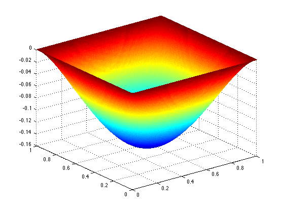
Figure 1. Test 3 $d=2,h=1/2^{7},\nu=50$

References

- [1] Awanou, G.: Pseudo transient continuation and time marching methods for Monge-Ampère type equations. http://arxiv.org/abs/1301.5891
- [2] Awanou, G.: Spline element method for the Monge-Ampère equation. http://arxiv.org/abs/1012.1775
- [3] Awanou, G.: Mixed finite element approximation of the Aleksandrov solution of the Monge-Ampère equation (In preparation)
- [4] Awanou, G.: Standard finite elements for the numerical resolution of the elliptic Monge-Ampère equation: Aleksandrov solutions (Manuscript)
- [5] Brenner, S.C., Gudi, T., Neilan, M., Sung, L.Y.: penalty methods for the fully nonlinear Monge-Ampère equation. Math. Comp. 80(276), 1979–1995 (2011)
- [6] Brenner, S.C., Neilan, M.: Finite element approximations of the three dimensional Monge-Ampère equation. ESAIM Math. Model. Numer. Anal. 46(5), 979–1001 (2012)
- [7] Brenner, S.C., Scott, L.R.: The mathematical theory of finite element methods, Texts in Applied Mathematics, vol. 15, second edn. Springer-Verlag, New York (2002)
- [8] Evans, L.C.: Partial differential equations, Graduate Studies in Mathematics, vol. 19. American Mathematical Society, Providence, RI (1998)
- [9] Feng, X., Neilan, M.: Error analysis for mixed finite element approximations of the fully nonlinear Monge-Ampère equation based on the vanishing moment method. SIAM J. Numer. Anal. 47(2), 1226–1250 (2009)
- [10] Glowinski, R.: Numerical methods for fully nonlinear elliptic equations. In: ICIAM 07—6th International Congress on Industrial and Applied Mathematics, pp. 155–192. Eur. Math. Soc., Zürich (2009)
- [11] Harris, G., Martin, C.: The roots of a polynomial vary continuously as a function of the coefficients. Proc. Amer. Math. Soc. 100(2), 390–392 (1987)
- [12] Lakkis, O., Pryer, T.: A finite element method for second order nonvariational elliptic problems. SIAM J. Sci. Comput. 33, 786–801 (2011)
- [13] Neilan, M.: Quadratic Finite Element Approximations of the Monge-Ampère Equation. J. Sci. Comput. 54(1), 200–226 (2013)
- [14] Ostrowski, A.M.: Solution of equations and systems of equations. Pure and Applied Mathematics, Vol. IX. Academic Press, New York-London (1960)