Simulation with Fluctuating and Singular Rates

Abstract

In this paper we present a method to generate independent samples for a general random variable, either continuous or discrete. The algorithm is an extension of the acceptance-rejection method, and it is particularly useful for kinetic simulation in which the rates are fluctuating in time and have singular limits, as occurs for example in simulation of recombination interactions in a plasma. Although it depends on some additional requirements, the new method is easy to implement and rejects less samples than the acceptance-rejection method.

1 Introduction

Kinetic transport for a gas or plasma involves particle interactions such as collisions, excitation/deexcitation and ionization/recombination. Simulation of these interactions is most often performed using the Direct Simulation Monte Carlo (DSMC) method [1] or one of its variants, in which the actual particle distribution is represented by a relatively small number of numerical particles, each of which is characterized by state variables, such as position $x$ and energy $E$. Interactions between the numerical particles are performed by random selection of the interacting particles and the interaction parameters, depending on the interaction rates. Correctly sampling these interactions involves several computational challenges: First the number $N$ of particles can be large (e.g., $N=10^{6}$) and the number of possible interaction events can be even larger (e.g., $N^{k}$ for $k=2$ or $3$). Second, the interaction probabilities vary throughout the simulation since interactions change the state of the interacting particles. These two difficulties are routinely overcome using acceptance-rejection sampling. Third, the interaction rates can be nearly singular, for example in a recombination event between an ion and two electrons (described in more detail in Section 5). This creates a wide range of interaction rates that makes acceptance-rejection computationally intractable. Figure 1 illustrates these challenges and how different methods can handle them. The sampling method presented here, which we call Reduced Rejection, was developed to overcome the challenges of a large number of interaction events with fluctuating and singular rates.

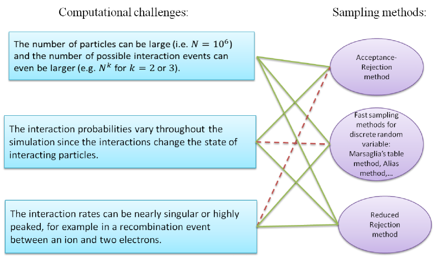
Figure 1: This figure illustrates the computational challenges involved in sampling interactions of numerical particles, and how different methods can handle them. Broken line represents challenges for which the method becomes computationally inefficient, whereas, the solid line represents the challenges for which the method is still computationally efficient.

Simulation of kinetics requires sampling methods that generate independent samples. This rules out Markov Chain Monte Carlo schemes, such as Metropolis–Hastings, Gibbs sampling, and Slice sampling. Although these methods are very powerful and are used very often, this paper focuses on sampling methods that generate independent samples.

There are several efficient algorithms for simulation of discrete random variables, notably Marsaglia’s table method [11] and the Alias method [19, 20]. However, these methods require pre-processing time and, therefore, are not efficient for sampling from a random variable whose probability function changes during the simulation. For continuous random variables there are several different algorithms; nevertheless, each of these algorithms has its own constraints. For example, Inverse Transform Sampling method requires knowledge of the cumulative distribution function and evaluation of its inverse, Box-Muller only applies to a normal distribution, and Ziggurat algorithm [12] can be used for random variables that have monotone decreasing (or symmetric unimodal) density function.

The algorithm of choice for general (both continuous and discrete) random variables that generates independent samples and does not require preprocessing time is acceptance-rejection method (see for example [3]). Let $q(x)$ be a real-valued function on the sample space. Let $I[q]$ denote the expectation of function $q(x)$. By sampling according to function $q(x)$ we mean to sample using the probability distribution function $q(x)/I[q]$. We say function $q(x)$ encloses function $p(x)$ if $p(x)\leq q(x)$ for all $x$ in the sample space. The idea of acceptance-rejection method is to find a proposal function $q(x)$ that encloses function $p(x)$. Suppose we already have a mechanism to sample according to $q(x)$, then acceptance-rejection algorithm enables us to sample according to $p(x)$. In most cases the constant function is used as the proposal function $q(x)$. The main drawback of acceptance-rejection method is that it might reject many samples. Indeed the ratio of the number of rejected samples to the number of accepted samples is approximately equal to the ratio of the area between curves $q(x)$ and $p(x)$ to the area under the curve $p(x)$.

For many given distributions, finding a good proposal function that encloses it without leading to many rejected samples is difficult. One extension to acceptance-rejection method is Adaptive Rejection Sampling [8]. The basic idea of Adaptive Rejection Sampling is to construct proposal function $q(x)$ that encloses the given distribution by concatenating segments of one or more exponential distributions. As the algorithm proceeds, it successively updates the proposal function $q(x)$ to correspond more closely to the given distribution. Another extension to Acceptance-rejection method is economical method [5]. This method is basically a generalization of Alias method for continuous distributions. In this method, one needs to define a specific transformation that maps $\{x:p(x)>q(x)\}$ to $\{x:p(x)\leq q(x)\}$. Although this method produces no rejection, finding the required transformation is difficult in general.

In the Reduced Rejection method we sample according to a given function $p(x)$ based on a proposal function $q(x)$. In contrast to the acceptance-rejection method, Reduced Rejection sampling does not require $q(x)$ to enclose $p(x)$ (i.e. it allows $p(x)>q(x)$ for some $x$). On the other hand, Reduced Rejection sampling requires some extra knowledge about the functions $p(x)$ and $q(x)$.

The Reduced Rejection sampling method can be applied to a wide range of sampling problems (for both continuous and discrete random variables) and in many examples is more efficient than customary methods (three examples are provided in sections 4, 5 and 6). In particular, Reduced Rejection sampling requires no pre-processing time and consequently is suitable for simulations in which $p(x)$ is changing constantly (see section 3 for an elaboration on this point and sections 5 and 6 for examples of simulations with fluctuating $p(x)$). Also in situations where $p(x)$ has singularities or is highly peaked in certain regions, Reduced Rejection sampling can be very efficient.

The next section describes the Reduced Rejection sampling and proves its validity. Section 3 compares Reduced Rejection sampling to other methods (including other generalizations of acceptance-rejection), highlights advantages of Reduced Rejection sampling in comparison to other methods, and points out some of the challenges in applying Reduced Rejection sampling. In section 4, Reduced Rejection sampling is demonstrated on a simple example. In section 5, Reduced Rejection sampling is applied to an example motivated from plasma physics, for which other sampling methods cannot be used efficiently. In section 6, we make some comments on how to apply Reduced Rejection in the context of stochastic chemical kinetics. In the appendix, we provide flow charts for the Reduced Rejection algorithm.

2 Reduced Rejection sampling

Consider a sample space $\Omega$ with Lebesgue measure $\mu$ on $\Omega$, and two functions $q,p:\Omega\rightarrow\mathbb{R}$. Denote

$$I[q]=\int_{\Omega}q(x)d\mu(x),\qquad I[p]=\int_{\Omega}p(x)d\mu(s).$$

By sampling from $\Omega$ according to $p(x)$ we mean sampling from $\Omega$ using probability distribution function $p(x)/I[p]$. Partition sample space $\Omega$ into two sets ${\it\mathcal{S}}$ and ${\it\mathcal{L}}$:

$$\mathcal{L}=\{x\in\Omega:p(x)>q(x)\},\qquad\mathcal{S}=\{x\in\Omega:p(x)\leq q(x)\}.$$

Reduced Rejection sampling is a method for sampling from $\Omega$ according to $p(x)$ using an auxiliary function $q(x)$. It depends on the following:

• The values of $I[q]$, $I[p]$ and $\int_{\mathcal{L}}(p(x)-q(x))d\mu(x)$. Note that the last value is needed only for “Algorithm II”, see subsection 2.1.

• A mechanism to sample from $\Omega$ according to $q(x)$.

• A mechanism to sample from $\mathcal{L}$ according to $p(x)-q(x)$.

Whereas the acceptance-rejection method for sampling from $p(x)$ requires a function $q(x)$ that encloses $p(x)$ (i.e., $0\leq p(x)\leq q(x)$ for all $x\in\Omega$), the Reduced Rejection sampling algorithm is a generalization of the acceptance-rejection method, that allows $p(x)>q(x)$ for some $x$. The Reduced Rejection sampling algorithm is detailed in Section 2.1, and its validity as a method for sampling from $\Omega$ according to $p(x)$ is demonstrated in Section 2.2.

2.1 The Reduced Rejection sampling algorithm

The Reduced Rejection sampling method consists of two algorithms (i.e., two different algorithms) depending on the relative values of $I[p]$ and $I[q]$. The outcome of each algorithm is a value $z$ that is an independent sample from $\Omega$ according to $p(x)$.

Algorithm I: $\mathbf{I[p]\geq I[q]}$.

Perform the following steps:

• With probability $(I[p]-I[q])/I[p]$, sample $x_{0}$ from $\mathcal{L}$ according to $p(x)-q(x)$ and accept $z=x_{0}$.

• Otherwise (with probability $(I[q]/I[p]$), sample $x_{0}$ from $\Omega$ according to $q(x)$.

  1. If $x_{0}\in\mathcal{L}$, accept $z=x_{0}$.

  2. If $x_{0}\in\mathcal{S}$, accept $z=x_{0}$ with probability $p(x_{0})/q(x_{0})$.

• If $x_{0}$ was not accepted, then sample a new value of $x_{1}$ from $\mathcal{L}$ according to $p(x)-q(x)$ and accept $z=x_{1}$.

Algorithm II: $\mathbf{I[p]<I[q]}$.

Perform the following steps until a value $z$ is accepted:

• Sample $x_{0}$ from $\Omega$ according to $q(x)$.

• If $x_{0}\in\mathcal{L}$, accept $z=x_{0}$.

• If $x_{0}\in\mathcal{S}$, accept $z=x_{0}$ with probability $p_{a}=p(x_{0})/q(x_{0})$,

• If $x_{0}$ was not accepted, then

  1. With probability $p_{a}$ select $x_{1}$ from $\mathcal{L}$ according to $p(x)-q(x)$ and accept $z=x_{1}$, in which

     $$p_{a} = \frac{\int_{\mathcal{L}}(p(x)-q(x))d\mu(x)}{\int_{\mathcal{S}}(q(x)-p(x))d\mu(x)}$$ (1)

     $$= \frac{\int_{\mathcal{L}}(p(x)-q(x))d\mu(x)}{I[q]-I[p]+\int_{\mathcal{L}}(p(x)-q(x))d\mu(x)}.$$

  2. Otherwise (i.e., with probability $1-p_{a}$), return to (i) without accepting a value of $z$.

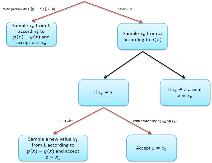
Figure 5: Flow chart of Algorithm I of the Reduced Rejection sampling method attributing to the case $I[p]\geq I[q]$.

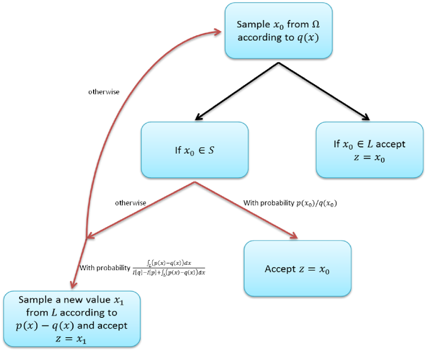
Figure 6: Flow chart of Algorithm II of the Reduced Rejection sampling method attributing to the case $I[p]<I[q]$.

Figures 5 and 6 in appendix A, illustrate flow charts of Algorithms I and II.

As described in Algorithms I and II, Reduced Rejection samples from $p$ through the following steps: On $\mathcal{L}$, treat $p$ as a mixture $p=q+(p-q)$ and sample from $q$ and $p-q$ with the correct probabilities; and on $\mathcal{S}$, sample from $p$ by sampling from $q$ and accepting the sample with probability $p/q$. Rejected samples in $\mathcal{S}$ correspond to the region $B$ in figure 2, and the region $A$ is where $q$ does not enclose $p$. If $|A|>|B|$ (i.e., Algorithm I) then all of the rejected samples can be replaced by samples from $A$; if $|A|<|B|$ (i.e., Algorithm II) then a portion of the rejected samples can be replaced by samples from $A$, and for the remainder, the algorithm is repeated as in Acceptance-Rejection.

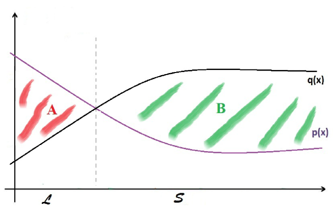
Figure 2: This figure illustrates the Reduced Rejection method. Region $A$ is where $q$ does not enclose $p$, and region $B$ is where samples are rejected. Rejected samples from region $B$ can be replaced by samples from region $A$ if $|A|>|B|$; otherwise (if $|A|<|B|$), some of the rejected samples lead to repetition of the algorithm.

2.2 Validity of Reduced Rejection Sampling

In this subsection we show the correctness of the Reduced Rejection sampling method. As the method is different for Algorithms I and II, we prove the correctness for each algorithm separately.

Proof for Algorithm I: For each $z\in\Omega$, show that the algorithm of Algorithm I returns $z$ with probability $p(z)d\mu(z)/I[p]$.

If $z\in\mathcal{S}$, then part (ii) must have been selected, $z$ must have been sampled in (ii) and it must have been accepted in case (ii.b). Therefore, the probability of returning $z$ is

$${\hbox{Pr}}[\hbox{(ii) selected}]\ {\hbox{Pr}}[z\hbox{ sampled in (ii)}]\ {\hbox{Pr}}[z\hbox{ accepted in (ii.b)}] = \frac{I[q]}{I[p]}\times\frac{q(z)d\mu(z)}{I[q]}\times\frac{p(z)}{q(z)}$$ (2)

$$= \frac{p(z)d\mu(z)}{I[p]}.$$

Also note that for every $x_{0}\in\mathcal{S}$, after $x_{0}$ is selected in (ii.b) with probability $\frac{q(x)}{I[q]}d\mu(x)$, the probability of reaching (iii) is $\frac{q(x_{0})-p(x_{0})}{q(x_{0})}$. Thus the total probability of reaching (iii) after selecting (ii) is

$${\hbox{Pr}}[\hbox{reaching (iii) $|$ (ii) selected}]=\int_{\mathcal{S}}\frac{q(x)-p(x)}{q(x)}\frac{q(x)}{I[q]}d\mu(x)=\frac{\int_{\mathcal{S}}(q(x)-p(x))d\mu(x)}{I[q]}.$$ (3)

Next suppose that $z\in\mathcal{L}$. The probability that $z$ is returned from (i) is

$${\hbox{Pr}}[z\hbox{ returned from (i)}]= {\hbox{Pr}}[\hbox{(i) selected}]\ {\hbox{Pr}}[z\hbox{ sampled in (i)}]$$

$$= \frac{(I[p]-I[q])}{I[p]}\times\frac{(p(z)-q(z))d\mu(z)}{\int_{\mathcal{L}}(p(x)-q(x))d\mu(x)}.$$ (4)

The probability that $z$ was returned from (ii.a) is

$${\hbox{Pr}}[z\hbox{ returned from (ii.a)}]= {\hbox{Pr}}[\hbox{(ii) selected}]\ {\hbox{Pr}}[z\hbox{ sampled in (ii.a)}]$$

$$= \frac{I[q]}{I[p]}\times\frac{q(z)d\mu(z)}{I[q]}$$

$$= \frac{q(z)d\mu(z)}{I[p]}.$$ (5)

Also, using equation (3), the probability that $z$ was returned from (iii) is

$${\hbox{Pr}}[z \hbox{ returned from (iii)}]$$

$$= {\hbox{Pr}}[\hbox{(ii) selected}]\ {\hbox{Pr}}[\hbox{reaching (iii) $|$ (ii) selected}]\ {\hbox{Pr}}[z\hbox{ sampled from $\mathcal{L}$ in (iii)}]$$

$$= \frac{I[q]}{I[p]}\times\left(\frac{\int_{\mathcal{S}}(q(x)-p(x))d\mu(x)}{I[q]}\right)\times\frac{(p(z)-q(z))d\mu(z)}{\int_{\mathcal{L}}(p(x)-q(x))d\mu(x)}$$

$$= \frac{\int_{\mathcal{S}}(q(x)-p(x))d\mu(x)}{I[p]}\frac{(p(z)-q(z))d\mu(z)}{\int_{\mathcal{L}}(p(x)-q(x))d\mu(x)}.$$ (6)

Finally, using equations (4), (5), and (6), the probability of returning $z$ is

$${\hbox{Pr}}[z \hbox{ returned from (i)}]+{\hbox{Pr}}[z\hbox{ returned from (ii.a)}]+{\hbox{Pr}}[z\hbox{ returned from (iii)}]$$

$$= \frac{(I[p]-I[q])}{I[p]}\frac{(p(z)-q(z))d\mu(z)}{\int_{\mathcal{L}}(p(x)-q(x))d\mu(x)}+\frac{q(z)d\mu(z)}{I[p]}+\frac{(p(z)-q(z))d\mu(z)}{\int_{\mathcal{L}}(p(x)-q(x))d\mu(x)}\frac{\int_{\mathcal{S}}(q(x)-p(x))d\mu(x)}{I[p]}$$

$$= \frac{(p(z)-q(z))d\mu(z)}{I[p]\int_{\mathcal{L}}(p(x)-q(x))d\mu(x)}\left(I[p]-I[q]+\int_{\mathcal{S}}(q(x)-p(x))d\mu(x)\right)+\frac{q(z)d\mu(z)}{I[p]}$$

$$= \frac{(p(z)-q(z))d\mu(z)}{I[p]\int_{\mathcal{L}}(p(x)-q(x))d\mu(x)}\left(\int_{\mathcal{L}}(p(x)-q(x))d\mu(x)\right)+\frac{q(z)d\mu(z)}{I[p]}$$

$$= \frac{p(z)d\mu(z)}{I[p]}.$$ (7)

Hence, by (2) and (7), whether $z\in\mathcal{S}$ or $z\in\mathcal{L}$, the probability of returning $z$ is equal to $p(z)d\mu(z)/I[p]$. This completes the proof for Algorithm I.  

Proof for Algorithm II: For each $z\in\Omega$, show that the algorithm in Algorithm II returns $z$ with probability $p(z)d\mu(z)/I[p]$. The algorithm consists of some number of cycles, each consisting of steps (i)-(iv), until a value $z$ is accepted. We first calculate the probability that $z$ is accepted within one of the cycles.

Suppose that $z\in\mathcal{S}$. Then $z$ must be sampled in (i) and accepted in (iii). Thus, the probability of returning $z$ in (iii) is

$${\hbox{Pr}}[z\hbox{ returned from (iii)}]= {\hbox{Pr}}[z\hbox{ sampled in (i)}]\ {\hbox{Pr}}[z\hbox{ accepted in (iii)}]$$

$$= \frac{q(z)d\mu(z)}{I[q]}\times\frac{p(z)}{q(z)}$$

$$= \frac{p(z)d\mu(z)}{I[q]}.$$ (8)

Also note that for every $x_{0}\in\mathcal{S}$,which is chosen with probability $\frac{q(x_{0})d\mu(x_{0})}{I[q]}$, the probability that it is not accepted in (iii) is $\frac{q(x_{0})-p(x_{0})}{q(x_{0})}$. Thus the total probability of not returning an element of $\mathcal{S}$ in (iii), which is the same as the probability of reaching (iv), is

$${\hbox{Pr}}[\hbox{reaching (iv)}]=\int_{\mathcal{S}}\frac{q(x)-p(x)}{q(x)}\frac{q(x)}{I[q]}d\mu(x)=\int_{\mathcal{S}}\frac{q(x)-p(x)}{I[q]}d\mu(x).$$ (9)

Next suppose that $z\in\mathcal{L}$. The probability that $z$ is accepted in (ii) is

$${\hbox{Pr}}[z\hbox{ returned from (ii)}]=\frac{q(z)d\mu(z)}{I[q]}.$$ (10)

For $z$ to be returned from (iv.a), the algorithm must reach (iv), then go to (iv.a) and then select $z$ in (iv.a). This has probability

$${\hbox{Pr}}[z \hbox{ returned from (iv.a)}]$$

$$= {\hbox{Pr}}[\hbox{reach (iv)}]\ {\hbox{Pr}}[\hbox{go to (iv.a)}]\ {\hbox{Pr}}[\hbox{z sampled in (iv.a)}]$$

$$= \left(\int_{\mathcal{S}}\frac{q(x)-p(x)}{I[q]}d\mu(x)\right)\times\frac{\int_{\mathcal{L}}(p(x)-q(x))d\mu(x)}{\int_{\mathcal{S}}(q(x)-p(x))d\mu(x)}\times\frac{(p(z)-q(z))d\mu(z)}{\int_{\mathcal{L}}(p(x)-q(x))d\mu(x)}$$

$$= \frac{(p(z)-q(z))d\mu(z)}{I[q]}.$$ (11)

Now using equations (10) and (11), the probability of returning $z$ in a cycle is

$${\hbox{Pr}}[z\hbox{ returned}]= {\hbox{Pr}}[z\hbox{ returned from (ii)}]+{\hbox{Pr}}[z\hbox{ returned from (iv.a)}]$$

$$= \frac{q(z)d\mu(z)}{I[q]}+\frac{(p(z)-q(z))d\mu(z)}{I[q]}$$

$$= \frac{p(z)d\mu(z)}{I[q]}.$$ (12)

Equations (8) and (12) imply that, whether $z\in\mathcal{S}$ or $z\in\mathcal{L}$, the probability that $z$ is returned in a cycle is $p(z)d\mu(z)/I[q]$. Integrating over all the samples in $\Omega$, we deduce that the probability that a sample is returned in a cycle is $I[p]/I[q]$. Consequently, probability that no sample point is returned in a cycle is $1-I[p]/I[q]$. Because the cycle is repeated until a sample point is returned, we conclude that the probability that the algorithm returns $z$ is equal to

$$\sum_{k=1}^{\infty}(1-\frac{I[p]}{I[q]})^{k-1}\frac{p(z)d\mu(z)}{I[q]}=\frac{p(z)d\mu(z)}{I[p]}.$$

This completes the proof for Algorithm II.  

Note that the efficiency of Algorithm II is nominally the same as acceptance rejection, i.e. the probability of a rejection is $1-I[p]/I[q]$. Actually it can be significantly better because $I[q]$ can be smaller, since $q<p$ is allowed. Also, note that if $I[p]=I[q]$, then Algorithms I and II are the same.

3 Comparison of Reduced Rejection and Other Sampling Methods

One of the important features of Reduced Rejection sampling is that it requires no preprocessing time. This is particularly useful for dynamic simulation; i.e., simulation in which the probability distribution function $p(x)$ may change after each sample (see section 5 for an example from plasma physics). For dynamic simulation, fast discrete sampling methods such as Marsaglia’s table method or the Alias method, are not suitable as they require preprocessing time after each change in $p(x)$. Although, the acceptance-rejection method requires no preprocessing time and can be used for dynamic simulation, it may require changes in $q(x)$ if $p(x)$ changes, which is usually not difficult, and it becomes very inefficient when the ratio of the area under function $p(x)$ to the area under proposal function $q(x)$ is small. Moreover, adaptive rejection sampling is not efficient, because the process of adapting $q(x)$ to $p(x)$ starts over whenever $p(x)$ changes.

The Reduced Rejection sampling method can be thought as an extension of the acceptance-rejection method. In particular when the proposal function $q(x)$ encloses $p(x)$ (i.e., $q(x)\geq p(x)\hbox{ for all }x\in\Omega$ so that $\mathcal{L}=\emptyset$) the Reduced Rejection sampling method reduces to acceptance-rejection method. The advantage of Reduced Rejection sampling over acceptance-rejection method is that the proposal function $q(x)$ does not need to enclose function $p(x)$; i.e., it allows $q(x)<p(x)$ for some $x$. This is very useful in dynamic simulation as it can accommodate changes in $p(x)$ without requiring changes in $q(x)$. Moreover, Reduced Rejection sampling may result in less unwanted samples than acceptance-rejection does, especially if $p(x)$ has singularities or is highly peaked.

There are several challenges in implementing the Reduced Rejection sampling method. The main challenge is the need to sample from set $\Omega$ according to $q(x)$ and from set $\mathcal{L}$ according to $p(x)-q(x)$, which can be performed by various sampling methods. Another challenge in using Reduced Rejection sampling is the need to know the values of $I[q]$, $I[p]$ and $\int_{\mathcal{L}}(p(x)-q(x))d\mu(x)$ (but note that the last value is only for Algorithm II). In many situations, these values are readily available or can be calculated during the simulation.

4 Example 1: Reduced Rejection Sampling for a Random Variable with Singular Density

In this section, Reduced Rejection sampling method is applied to a simple problem. Let $\Omega=(0,1)$ and sample according to

$$p(x)=\frac{1}{\sqrt{x}}+\frac{1}{\sqrt[5]{1-x}}$$ (13)

which has singularities at 0 and 1. Using inverse transform sampling, it is easy to sample according to $1/\sqrt{x}$ or $1/\sqrt[5]{1-x}$, but inverse transform cannot be easily applied to (13) as it requires finding the root of a eighth degree polynomial. We apply Reduced Rejection sampling to this problem by setting $q(x)=1/\sqrt{x}$. Observe that $\mathcal{L}=\Omega=(0,1)$. As mentioned earlier, inverse transform sampling is easily used to sample according to $q(x)$ and according to $p(x)-q(x)$. The Reduced Rejection sampling is very fast and yields no unwanted sample points. This example is equivalent to sampling from a mixture and can be extended to sampling from a probability density $p(x)$ that is a sum $p=p_{1}+p_{2}+\ldots+p_{n}$, if there is a method for sampling from each $p_{k}$ separately and the integrals $I[p_{k}]$ are all known.

5 Example 2: Reduced Rejection Sampling for a Stochastic Process with Fluctuating and Singular Rates

In this section, we apply Reduced Rejection sampling to an idealized problem motivated by plasma physics. As discussed in subsection 5.5, the unique features of this problem makes other sampling methods inefficient to use.

5.1 Statement of the Stochastic Process and the Simulation Algorithm

The example presented here is a simplified version of simulation for recombination by impact of two electrons with an ion, in which one of the electrons is absorbed into the atom and the other electron is scattered. For incident electron energies $E_{1}$ and $E_{2}$, the recombination rate is proportional to $(E_{1}E_{2})^{-1/2}$ [15, 21], which can become singular if electrons of low energy are present. This is an obstacle to kinetic simulation of recombination by electron impact in a plasma.

Our goal is to simulate the evolution of the following system: Consider $N$ particles labeled $1,\ldots,N$. To each particle $i$ we associate a number $x_{i}\in(0,1)$, called the state of particle $i$ (and corresponding to electron energy in the recombination problem). Occasionally, where it does not cause confusion, we use $x_{i}$ to refer to particle $i$. We refer to the set $\Gamma=\{x_{1},\ldots,x_{n}\}$ as the configuration of the system. For every pair of states $x_{i}$ and $x_{j}$, $T_{i,j}$ is a random variable with an exponential distribution with parameter $(x_{i}x_{j})^{\alpha}$, in which $\alpha$ is a fixed constant between 0 and 1. $T_{i,j}$ is the time for interaction between particle $i$ and $j$ which randomly occurs with rate $1/(x_{i}x_{j})^{\alpha}$. After an interaction occurs, say for the pair $\{k,l\}$, the values of states $x_{k}$ and $x_{l}$ are replaced by new values $x^{\prime}_{k}$ and $x^{\prime}_{l}$; consequently, the distribution of $T_{i,j}$ changes if either of $i$ and $j$ is equal to $k$ or $l$.

We will consider a simple updating mechanisms for the states after each interaction. In the simulations presented below, the updated values of $x^{\prime}_{k}$ and $x^{\prime}_{l}$ are chosen independently and uniformly at random from $(0,1)$, without dependence on $x_{k}$ and $x_{l}$. This choice has been made for simplicity and because the stationary distribution can be calculated for this choice (see section 5.2), but we expect that Reduced Rejection sampling would work equally well for more complex interaction rules. Indeed the algorithm 5.1 described below and the more detailed algorithm presented in section 5.4 do not depend on the interaction rules.

First we make some notation and observations. Set $s_{i}=1/x_{i}^{\alpha}$ and $s=\sum_{i}s_{i}$. Let $T(\lambda)$ denotes an exponential random variable with parameter $\lambda$ (with rate $1/\lambda$); then $T(\lambda)=\mu T(\mu\lambda)$ for any scalar $\mu$. We will use

$$\frac{s_{i}}{s}\frac{s_{j}}{s}T(1/s^{2})=T(1/(s_{i}s_{j}))$$

in the following algorithm, which is a variant of the Kinetic Monte Carlo (KMC) algorithm (also known as the residence-time algorithm or the n-fold way or the Bortz-Kalos-Lebowitz (BKL) algorithm [2]), that simulates the system described above. This algorithm chooses interactions, by choosing two particles separately out of the $N$ number of particles, rather than choosing a pair of particles out of the $N^{2}$ number of pairs.

Algorithm 5.1

1. Start from $t=0.$

2. Choose time $\Delta t$ by sampling from an exponential distribution with rate $s^{2}$.

3. Choose index $k$ with probability $s_{k}/s$.

4. Choose index $l$ with probability $s_{l}/s$.

5. At time $t+\Delta t$ interaction between particles $k$ and $l$ occurs.

6. Update states $x_{k}$ and $x_{l}$ according to the updating mechanism and the update value of $s$.

7. Set $t=t+\Delta t$ and start over from 2.

We use Reduced Rejection sampling in subsection 5.5 to perform steps 3 and 4 in the above algorithm. We also explain why other methods of sampling would be inefficient in this circumstances. To verify that our simulation is working properly, we perform the following test.

Let $g(x_{1},\ldots,x_{N})$ be a real-valued function on configuration space, with expectation $E[g]$ of $g$ over configurations of the system. For a simple interaction rule and some functions $g$ we can find the value of $E[g]$ analytically, as shown in subsection 5.2. Consequently, the difference between the numerical and analytic results provides a measure of the accuracy of the simulation as discussed at the end of subsection 5.5.

5.2 Theoretical results

Think of the system’s evolution as a random walk over the configurations of the system. Suppose the updating process is that if states $x_{k}$ and $x_{l}$ interact, then states $x^{\prime}_{k}$ and $x^{\prime}_{l}$ are chosen, independently, uniformly at random from $(0,1)$. In this section, we find the stationary distribution for this random walk and the value of $E[g]$ for two functions $g$.

Let $P(\Gamma^{\prime}|\Gamma)$ denote the probability of going from configuration $\Gamma$ to configuration $\Gamma^{\prime}$, and $P(x^{\prime}_{k},x^{\prime}_{l}|x_{k},x_{l})$ as the probability of going from values $x_{k},x_{l}$ to values $x^{\prime}_{k},x^{\prime}_{l}$ in an interaction. These satisfy

$$P(x^{\prime}_{k},x^{\prime}_{l}|x_{k},x_{l})=P(x_{k},x_{l}|x^{\prime}_{k},x^{\prime}_{l}),$$ (14)

that is, the probability of getting $x^{\prime}_{k}$ and $x^{\prime}_{l}$ after $x_{k}$ and $x_{l}$ interact, is the same as probability of getting $x_{k}$ and $x_{l}$ after $x^{\prime}_{k}$ and $x^{\prime}_{l}$ interact. Furthermore, for this updating mechanism, the random walk is completely mixing; that is, it can go from any configuration to any other configuration (If for example the updating mechanism had additional constraints, such as ${x^{\prime}_{k}}+{x^{\prime}_{l}}=x_{k}+x_{l}$, then we would not have a mixing random walk since we could reach only those configurations that have the same sum of states as the starting configuration).

For every configuration $\Gamma=\{x_{1}\ldots,x_{N}\}$, set

$$\pi_{\Gamma}:=\frac{(x_{1}\cdots x_{N})^{\alpha}}{Z}\left(\sum_{i,j}\frac{1}{(x_{i}x_{j})^{\alpha}}\right),$$

where $Z$ is the normalizing constant so that $\sum_{\Gamma}\pi_{\Gamma}=1$.

Suppose the current configuration of the system is $\Gamma=\{x_{1},\ldots,x_{N}\}$. According to steps 3 and 4 in algorithm 5.1, the probability of interaction occurring between states $x_{k}$ and $x_{l}$ is proportional to $s_{k}s_{l}=1/(x_{k}x_{l})^{\alpha}$. Let $\Gamma^{\prime}=\{x^{\prime}_{k},x^{\prime}_{l}\}\cup\Gamma\setminus\{x_{k},x_{l}\}$. Then

$$P(\Gamma^{\prime}|\Gamma)=\frac{1/(x_{k}x_{l})^{\alpha}}{\sum_{i,j}1/(x_{i}x_{j})^{\alpha}}P(x^{\prime}_{k},x^{\prime}_{l}|x_{k},x_{l}).$$

For the ease of explanation, relabel the states of $\Gamma^{\prime}$ so that $\Gamma^{\prime}=\{x^{\prime}_{1},\ldots,x^{\prime}_{N}\}$ where $x^{\prime}_{i}=x_{i}$ for $i\neq k,l$. Similarly,

$$\pi_{\Gamma^{\prime}}=\frac{(x^{\prime}_{1}\cdots x^{\prime}_{N})^{\alpha}}{Z}\left(\sum_{i,j}\frac{1}{(x^{\prime}_{i}x^{\prime}_{j})^{\alpha}}\right),\quad\hbox{ and }\quad P(\Gamma|\Gamma^{\prime})=\frac{1/(x^{\prime}_{k}x^{\prime}_{l})^{\alpha}}{\sum_{i,j}1/(x^{\prime}_{i}x^{\prime}_{j})^{\alpha}}P(x_{k},x_{l}|x^{\prime}_{k},x^{\prime}_{l}).$$

Because of (14) and since $x^{\prime}_{i}=x_{i}$, for $i\neq k,l$, it is straightforward to verify the detailed balance equation

$$\pi_{\Gamma}P(\Gamma^{\prime}|\Gamma)=\pi_{\Gamma^{\prime}}P(\Gamma|\Gamma^{\prime}).$$

Therefore, $\pi_{\Gamma}$ is the (unique) stationary distribution of the random walk. Since the updating mechanism is completely mixing, the normalizing constant $Z$ for distribution $\pi_{\Gamma}$ is the integral

$$Z=\int_{(0,1)^{N}}(x_{1}\cdots x_{N})^{\alpha}\left(\sum_{i,j}\frac{1}{(x_{i}x_{j})^{\alpha}}\right)dx_{1}\cdots dx_{N}=\frac{\binom{N}{2}}{(\alpha+1)^{N-2}}.$$

Hence for any function $g(x_{1},\ldots,x_{N})$,

$$E[g]=\frac{(\alpha+1)^{N-2}}{\binom{N}{2}}\int_{(0,1)^{N}}g(x_{1},\ldots,x_{N})(x_{1}\cdots x_{N})^{\alpha}\left(\sum_{i,j}\frac{1}{(x_{i}x_{j})^{\alpha}}\right)dx_{1}\cdots dx_{N}.$$

Some tedious algebra leads to the following proposition:

Proposition 5.2

Using the above notations and assumptions:

• $E[g]=\frac{\alpha+1}{\alpha+2}(N-2)+1$ when $g(x_{1},\ldots,x_{N})=x_{1}+\cdots+x_{N}$.

• $E[g]=\frac{\alpha+1}{\alpha+3}(N-2)+\frac{2}{3}$ when $g(x_{1},\ldots,x_{N})=x^{2}_{1}+\cdots+x^{2}_{N}$.

5.3 Simulation issues

In this section we make some remarks about the challenges involved in simulating this system.

The main challenge of sampling in this dynamic simulation is that the $s_{i}$’s are changing after each interaction. Consequently, the sampling method should require small or zero preprocessing time. For this reason, discrete sampling methods such as Marsaglia’s table method or the Alias method are not very efficient for this problem.

Next consider using acceptance-rejection method based on uniform sampling from $1$ to $n$ for the proposal distribution (i.e., $q$ constant). As mentioned earlier, the changing distribution property of the problem is not very detrimental for acceptance-rejection. On the other hand, the singularity in the rates at $x_{i}=0$ can lead to a large constant for $q$, for which there will be many rejected samples, so that the method is inefficient. Moreover, there seems to be no other clear choice for the proposal distribution $q$ other than a constant. Note that the sampling is from a discrete set of probabilities $s_{i}/s$ with little control over their values; for example the $s_{i}$’s are not monotonically ordered. This is quite different from sampling a single random variable from the density $p(x)=x^{-\alpha}$.

5.4 Use of the Reduced Rejection algorithm

In this section we explain how to use Reduced Rejection Sampling to perform steps 3 and 4 in algorithm 5.1. Reduced Rejection sampling can be readily used in this dynamic simulation. Even though the values of the $s_{i}$’s change after each interaction, they do not change drastically; in each interaction at most two of the $s_{i}$’s change. Starting at time $0$, we set $q_{i}=p_{i}=s_{i}$. After each interaction, we update the values of $p_{i}$’s to $p_{i}=s_{i}$, but do not change the values of $q_{i}$’s. Note that we can easily update the value of $I[p]$ after each interaction and keep track of set $\mathcal{L}=\{i:p_{i}>q_{i}\}$ by comparing the updated values of $p_{i}$’s to their corresponding values of $q_{i}$’s. Moreover, the size of set $\mathcal{L}$ changes by at most 2 after each interaction (but it can also decrease after some interactions).

We use Marsaglia’s table method to sample according to $q_{i}$’s. Since we do not update $q_{i}$’s after each interaction, the preprocessing time in Marsaglia’s table method is only required for the first sampling and not for the subsequent samplings. To sample from set $\mathcal{L}$ according to $p_{i}-q_{i}$, we use acceptance-rejection with uniform distribution for the proposal distribution. As long as the size of set $\mathcal{L}$ is not too big, the sampling from $\mathcal{L}$ is not very time consuming. To prevent $\mathcal{L}$ from getting too large, we reset the values of $q_{i}$’s to $q_{i}=p_{i}=s_{i}$, which sets $\mathcal{L}$ to be empty, whenever the size of $\mathcal{L}$ exceeds a predetermined number $M$.

The size of $M$ is important for the performance of the algorithm. If $M$ is too small, then there are many updates of the $q_{i}$’s, each of which requires preprocessing time for Marsaglia’s table method. On the other hand, if $M$ is too big, then $\mathcal{L}$ is large and costly to sample from by acceptance-rejection. Our computational experience shows that setting $M$ equal to a multiple of $\sqrt{N}$ is a good choice. It might be better for the reinitialization criterion to be based on the efficiency of the sampling from $\mathcal{L}$ (i.e., the fraction of rejected samples when using acceptance rejection on $\mathcal{L}$), rather than the size of $\mathcal{L}$.

5.5 Numerical result

We simulated the evolution of the system under the conditions outlined in subsection 5.2 with $N=10^{4}$, and $\alpha=0.5$. We start with a random configuration at time $t=0$. The simulation is based the Reduced Rejection sampling method, using Marsaglia’s table method and the acceptance-rejection method as described above. After each interaction, we evaluate function $g(x_{1},\ldots,x_{N})=x_{1}+\cdots+x_{N}$ and take the average to get an estimate for $E[g]$. Each result is produced by taking an average of five independent runs. Figure 3 compares the results for $E[g]$ from Reduced Rejection sampling with those from the acceptance-rejection method. The results of figure 3 show excellent agreement between the values of $E[g]$ as a function of the number of interactions from the two methods, which provides a validity check for Reduced Rejection sampling.

The advantage of Reduced Rejection sampling is demonstrated in figure 4 which shows a log-log plot of the processing time, as a function of the number of interactions, for Reduced Rejection sampling and acceptance-rejection. The results show that Reduced Rejection sampling is much faster than the acceptance-rejection method. In fact, for $n$ interactions, the computational time scales like $O(n)$ for Reduced Rejection sampling, and like $O(n^{3/2})$ for acceptance-rejection, in the range $10^{4}\leq n\leq 10^{6}$. For small values of $n$, the initial pre-processing step of Marsaglia’s table method dominates the computational time. For $n>10^{4}$, however, the pre-processing time (including the multiple pre-processing steps due to reinitialization) is not a significant part of the computational time. The average number of reinitializations for Reduced Rejection sampling is $(0,0,0,3.7,53.1)$ for $n=(10^{2},10^{3},10^{4},10^{5},10^{6})$, respectively. Another interesting advantage of the Reduced Rejection sampling is that the variance of the processing time for independent runs is much smaller in the Reduced Rejection sampling than it is in the acceptance-rejection method.

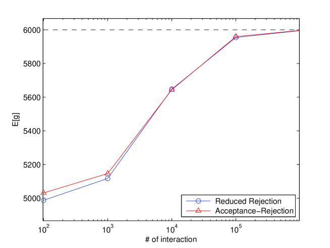
Figure 3: Theoretical (dashed line) and estimated values (solid lines) of $E[g]$ using different number of interactions. Here $g(x_{1},\ldots,x_{N})=x_{1}+\cdots+x_{N}$, $N=10^{4}$, and $\alpha=0.5$. Also $M=4000$ for the Reduced Rejection sampling. The theoretical value of $E[g]$ is 5999.8. The estimated value of $E[g]$ after $10^{6}$ interactions using Reduced Rejection sampling and acceptance-rejection methods were, respectively, 5994.59 and 5996.35. The reported result is the average of 5 independent runs.

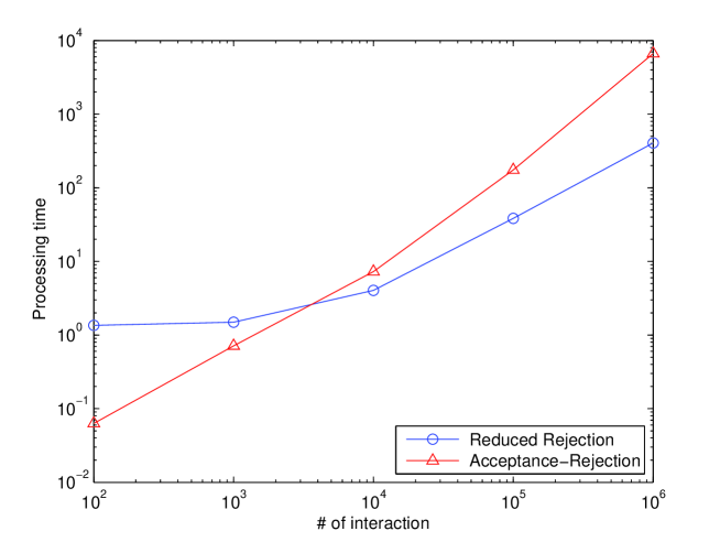
Figure 4: Loglog plot of the processing time for acceptance-rejection and Reduced Rejection sampling. Here $g(x_{1},\ldots,x_{N})=x_{1}+\cdots+x_{N}$, $N=10^{4}$ and $\alpha=0.5$. Also $M=4000$ for the Reduced Rejection sampling. The reported processing time is the average of 5 independent runs.

6 Example 3: Stochastic Simulation of Chemical Kinetics

In this section we describe how we can use Reduced Rejection in the context of stochastic chemical kinetics. Stochastic simulation in chemical kinetics is a Monte Carlo procedure to numerically simulate the time evolution of a well-stirred chemically reacting system. The first Stochastic Simulation Algorithm, called the Direct Method, was presented in [10]. The Direct Method is computationally expensive and there have been many adaptations of this algorithm to achieve greater speed in simulation. The first-reaction method, also in [10], is an equivalent formulation of the Direct Method. The next-reaction method [6] is an improvement over the first-reaction method, using a binary-tree structure to store the reaction times. The Modified Direct Method [4] and Sorting Direct Method [14] speed up the Direct Method by indexing the reactions in such a way that reactions with larger propensity function tend to have a lower index value. Recently, some new Stochastic Simulation Algorithms, called partial-propensity methods, were introduced that work only for elementary chemical reactions (i.e. reactions with at most two different reactants) (see [16, 17, 18]). Nevertheless, note that it is possible to decompose any non-elementary reaction into combination of elementary reactions. There are also approximate Stochastic Simulation Algorithms, such as tau-leaping and slow-scale, that provide better computational efficiency in exchange for sacrificing some of the exactness in the Direct Method (see [9] and the references therein for more details).

Next we give a brief review of stochastic simulation in chemical kinetics. An excellent reference with more detailed explanation is [9]. Using the same notation and terminology as in [9], consider a well-stirred system of molecules of $N$ chemical species $\{S_{1},\ldots,S_{N}\}$, which interact through $M$ chemical reactions $\{R_{1},\ldots,R_{M}\}$. Let $X_{i}(t)$ denote the number of molecules of species $S_{i}$ in the system at time $t$. The goal is to estimate the state vector ${\bf{X}}(t)\equiv(X_{1}(t),\ldots,X_{N}(t))$ given the system is initially in state ${\bf{X}}(0)={\bf{x}}_{0}$.

Similar to section 5, when the system is in state ${\bf{x}}$, the time for reaction $R_{j}$ to occur is given by an exponential distribution whose rate is the propensity function $a_{j}({\bf{x}})$. When reaction $R_{j}$ occurs, the state of the system changes from ${\bf{x}}$ to ${\bf{x}}+(v_{1j},\ldots,v_{Nj})$, where $v_{ij}$ is the change in the number of $S_{i}$ molecules when one reaction $R_{j}$ occurs.

Estimating the propensity functions in general is not an easy task. As noted, the value of the propensity functions depend on the state of the system. For example, if $R_{i}$ and $R_{j}$ are, respectively, the unimolecular reaction $S_{1}\rightarrow product(s)$ and bimolecular reaction $S_{1}+S_{2}\rightarrow product(s)$, then $a_{i}({\bf{x}})=c_{i}x_{1}$ and $a_{j}({\bf{x}})=c_{j}x_{1}x_{2}$ for some constants $c_{i}$ and $c_{j}$. Therefore, the propensity functions of the reactions are changing throughout the simulation. Moreover, if for some chemical species the magnitude of their population differ drastically from others, we expect the value of propensity functions to be very non-uniform.

For every state ${\bf{x}}$, define

$$a({\bf{x}})=\sum_{i=1}^{M}a_{i}({\bf{x}}).$$

To simulate the chemical kinetics of the system the following algorithm is used, which resembles algorithm 5.1 in section 5.

Algorithm 6.1

1. Start from time $t=0$ and state ${\bf{x}}={\bf{x}}_{0}$.

2. Choose time $\Delta t$ by sampling from an exponential distribution with rate $a({\bf{x}})$.

3. Choose index $k$ with probability $a_{k}({\bf{x}})/a({\bf{x}})$.

4. At time $t+\Delta t$ reaction $R_{k}$ occurs.

5. Update time $t=t+\Delta t$, state ${\bf{x}}={\bf{x}}+(v_{1k},\ldots,v_{Nk})$ and start over from 2.

In the original Direct Method [10] step 3 in the above algorithm 6.1 is performed by choosing number $r$ uniformly at random in the unit interval and setting

$$k=\hbox{ the smallest integer satisfying }\sum_{i=1}^{k}a_{i}({\bf{x}})>ra({\bf{x}}).$$ (15)

However, when we have many reactions with a wide range of propensity function values presented in the system, a scenario that is very common in biological models, the above procedure of using partial sums becomes computationally expensive. As noted earlier, some methods, such as the Modified Direct Method [4] and Sorting Direct Method [14], index the reactions in a smart way so that they can save on the average number of terms summed in equation (15) and consequently achieve computational efficiency.

We propose a different approach to performing step 3 in algorithm 6.1 using the acceptance-rejection or Reduced Rejection method. The approach is very similar to what was done in section 5. To be specific, we can use acceptance-rejection for step 3 in the following way: let

$$\bar{a}({\bf{x}})=\max_{i}a_{i}({\bf{x}}).$$

Until an index is accepted, select index $k$ uniformly at random from $\{1,\ldots,N\}$ and accept it with probability $a_{k}({\bf{x}})/\bar{a}({\bf{x}})$; otherwise, discard $k$ and repeat. When an index is accepted step 3 in algorithm 6.1 is completed. Typically for chemical reactions $R_{j}$, most of $v_{ij}$’s are zero; therefore, we can efficiently update the value of $\bar{a}({\bf{x}})$ at each iteration of algorithm 6.1.

However, as in section 5, if the values of $a_{i}({\bf{x}})$’s are very non-uniform (for example, when the population of some chemical species differ drastically from that of other species in the system) the acceptance-rejection method becomes inefficient due to rejection of many samples. In these circumstances, the Reduced Rejection algorithm can be readily used in a very similar way as it was used in section 5. We expect that the use of the Reduced Rejection algorithm in these circumstances would greatly improve the computational efficiency of the exact Stochastic Simulation Algorithms.

7 Conclusions and Future Directions

In this paper we introduce a new Reduced Rejection sampling method that can be used to generate independent samples for a discrete or continuous random variable. The strength of this algorithm is most evident for applications in which acceptance-rejection method is inefficient; namely, the probability distribution of the random variable is highly peaked in certain regions or has singularities. It is also useful when the probabilities are fluctuating, so that discrete methods that requiring preprocessing are inefficient. In particular, the Reduced Rejection sampling method is expected to perform well on kinetic simulation of electron-impact recombination in a plasma, which is difficult to simulate by other methods.

The preliminary examples in this paper are meant to illustrate these advantages of the Reduced Rejection sampling method. They provide evidence of improvement in computation time using the Reduced Rejection sampling versus acceptance-rejection method. These examples also provide some insights on implementation of the method.

One possible direction for future research is the nested use of Reduced Rejection sampling methods. For the most difficult step - sampling from $\mathcal{L}$ according to $p(x)-q(x)$ - we propose to apply the Reduced Rejection sampling method again using a new proposal function. In essence, this would use one Reduced Rejection sampling method inside another Reduced Rejection sampling method.

Appendix A Flow Charts of the Reduced Rejection Algorithm

References

- [1] G. A. Bird, Molecular Gas Dynamics and the Direct Simulation of Gas Flows, Claredon, Oxford (1994)
- [2] A.B. Bortz, M.H. Kalos, and J.L. Lebowitz. “A new algorithm for Monte Carlo simulation of Ising spin systems”, J. Comp. Phys. 17 (1975), 10-18.
- [3] R.E. Caflisch. “Monte Carlo and Quasi-Monte Carlo Methods”, Acta Numerica (1998), 1–49.
- [4] Y. Cao, H. Li, L.R. Petzold, “Efficient formulation of the stochastic simulation algorithm for chemically reacting systems”, J. Chem. Phys., 121, (2004), 4059–4067.
- [5] I. Deak. “An Economical Method for Random Number Generation and a Normal Generator”, Computing 27 (1981), 113–121.
- [6] M.A. Gibson, J. Bruck, “ Exact stochastic simulation of chemical systems with many species and many channels”, J. Phys. Chem., 105, (2000), 1876–1889.
- [7] W. R. Gilks, N. G. Best, and K. K. C. Tan, “Adaptive rejection Metropolis sampling”, Applied Statistics, 44, (1995), 455–472.
- [8] W. R. Gilks and P. Wild, “Adaptive rejection sampling for Gibbs sampling”, Applied Statistics, 41, (1992), 337–348.
- [9] D.T. Gillespie, “Stochastic Simulation of Chemical Kinetics”, Annu. Rev. Phys. Chem., 58, (2007), 35–55.
- [10] D.T. Gillespie, “A general method for numerically simulating the stochastic time evolution of coupled chemical reactions”, J. Comput. Phys., 22, (1976), 403–434.
- [11] G. Marsaglia, W. W. Tsang, and J. Wang, “Fast Generation of Discrete Random Variables”, Journal of Statistical Software, 11, 3 (2004).
- [12] G. Marsaglia and W. W. Tsang, “A fast, easily implemented method for sampling from decreasing or symmetric unimodal density functions”, SIAM Journ. Scient. and Statis. Computing, 5, 2 (1984), 349–359.
- [13] G. Marsaglia, “Xorshift RNGs”, Journal of Statistical Software, 8, 14 (2003).
- [14] J.M. McCollum, G.D. Peterson, C.D. Cox, M.L. Simpson, N.F. Samatova, “The sorting direct method for stochastic simulation of biochemical systems with varying reaction execution behavior”, Comput. Bio. Chem., 30, (2006), 39–49.
- [15] J.T. Oxenius, Kinetic Theory of Particles and Photons (1986) Springer-Verlag, Berlin.
- [16] R. Ramaswamy, N. Gonzalez-Segredo, I. F. Sbalzarini, “A new class of highly efficient exact stochastic simulation algorithms for chemical reaction networks”, J. Chem. Phys., 130, 244104, (2009).
- [17] R. Ramaswamy, I. F. Sbalzarini, “A partial-propensity variant of the composition-rejection stochastic simulation algorithm for chemical reaction networks”, J. Chem. Phys., 132, 044102, (2010).
- [18] R. Ramaswamy, I. F. Sbalzarini, “A partial-propensity formulation of the stochastic simulation algorithm for chemical reaction networks with delays”, J. Chem. Phys., 134, 014106, (2011).
- [19] M. D. Vose, “A Linear Algorithm For Generating Random Numbers With a Given Distribution”, IEEE Transaction and Software Engineering, 17, 9 (1991), 972–975.
- [20] A. J. Walker. “An efficient method for generating discrete random variables with general distributions”, ACM TOMS 3 (1977), 253–256.
- [21] Y.B. Zeldovich and Y.P. Raizer, Physics of Shock Waves and High-Temperature Hydrodynamic Phenomena (2002) Dover, Mineola, NY.