Measuring Metallicities with HST/WFC3 photometry

Abstract

We quantified and calibrated the metallicity and temperature sensitivities of colors derived from nine Wide Field Camera 3 (WFC3) filters aboard the Hubble Space Telescope (HST) using Dartmouth isochrones and Kurucz atmospheres models. The theoretical isochrone colors were tested and calibrated against observations of five well studied galactic clusters: M92, NGC 6752, NGC 104, NGC 5927, and NGC 6791, all of which have spectroscopically determined metallicities spanning $-2.30<$ [Fe/H] $<+0.4$. We found empirical corrections to the Dartmouth isochrone grid for each of the following color magnitude diagrams (CMD) (F555W–F814W, F814W), (F336W–F555W, F814W), (F390M–F555W, F814W) and (F390W–F555W, F814W). Using the empirical corrections we tested the accuracy and spread of the photometric metallicities assigned from CMDs and color-color diagrams (which are necessary to break the age-metallicity degeneracy). Testing three color-color diagrams [(F336W–F555W),(F390M–F555W),(F390W–F555W), vs (F555W–F814W)], we found the colors (F390M–F555W) and (F390W–F555W), to be the best suited to measure photometric metallicities. The color (F390W–F555W) requires much less integration time, but generally produces wider metallicity distributions, and, at very-low metallicity, the MDF from (F390W–F555W) is $\sim$60$\%$ wider than that from (F390M–F555W). Using the calibrated isochrones we recovered the overall cluster metallicity to within $\sim$ 0.1 dex in [Fe/H] when using CMDs (i.e. when the distance, reddening and ages are approximately known). The measured metallicity distribution function (MDF) from color-color diagrams show this method measures metallicities of stellar clusters of unknown age and metallicity with an accuracy of $\sim$ 0.2 - 0.5 dex using F336W–F555W, $\sim$0.15 - 0.25 dex using F390M–F555W, and $\sim$0.2 - 0.4 dex with F390W–F555W, with the larger uncertainty pertaining to the lowest metallicity range.

1. Introduction

Metallicity, age and mass are fundamental characteristics of a stellar population. Metallicity distributions, in conjunction with chemical evolution models, provide evolutionary information about both enrichment and gas inflow and outflow in the form of galactic winds. While in recent years measuring large numbers of spectroscopic metallicities has become more feasible with multiobject spectrographs (Kirby et al., 2011), it is still challenging to observe samples large enough to find rare objects or substructure in metallicity distribution functions, or to observe faint enough to build up large samples in nearby galaxies. Photometric metallicities, though not as accurate as spectra, provide measurements for every star in the field, including those with fainter magnitudes than can be reached spectroscopically.

The general technique to assign photometric metallicities relates color to metallicity. For instance, in a color magnitude diagram (CMD) fiducial ridgelines from several clusters with similar age, and a range of known metallicities can be interpolated to estimate the metallicity of an unmeasured cluster based upon the location of its ridgeline, provided that the cluster is also of similar age (e.g., Saviane et al. 2000; Da Costa et al. 2000,2002). Fiducial ridgelines have been used to derive empirical relations between color and metallicity at a given absolute magnitude (Da Costa & Armandroff, 1990; Calamida et al., 2007). Alternatively, one can use theoretical isochrones, however, the isochrones need to be empirically calibrated to match observed sequences (e.g., Brown et al. 2005; Lianou et al. 2011).

An issue with deriving metallicities from color arises because a giant can be redder either because it is older, or because it is more metal rich. One method to break the age-metallicity degeneracy uses a color-color diagram, where one color is constructed using a metallicity sensitive filter, and the other color is constructed from a pair of filters that provide a temperature estimate with minimal dependence on metallicity.

There is a long history in astronomy of using specifically designed filters to isolate stellar characteristics such as metallicity. Strömgren (1966) proposed photometric indices as a means of stellar classification. The $m_{1}=(v-b)-(b-y)$ index estimates the stellar metallicity of horizontal branch, red giant branch and main sequence stars when used in conjunction with a temperature-sensitive index such as $(b-y)$. The Washington system was developed to measure photometric metallicities, temperatures and the amount of CN line blanketing for giant G and K stars (Canterna, 1976).

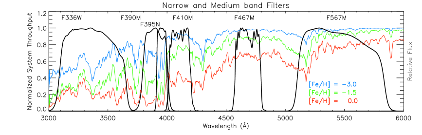
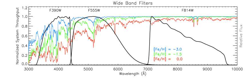
Figure 1.— UVIS filter transmission curves overlaid with Kurucz model stellar spectra of typical giant branch stars from log g = 1.5, T = 4000 and [Fe/H] = 0.0, -1.5, $\&$ -3.0. (A color version of this figure is available in the online journal.)

Another consideration with photometric metallicities is that medium and broad band colors lose nearly all sensitivity at low metallicity. The Caby system, developed in the 1990’s, modified the Strömgren system, replacing the v filter with a filter centered on the Ca H $\&$ K lines. The Caby system measures stellar metallicities 3 times more accurately, especially at low metallicity where the m₁ index loses sensitivity (Anthony-Twarog et al., 1991).

Several filters on the HST/WFC3 were designed to provide information on the metallicities of resolved populations. Our WFC3 calibration program (11729, PI Holtzman) was designed to collect images of clusters with well established spectroscopic metallicities in order to map WFC3 colors to metallicity. Another program designed to study the galactic bulge (11664, PI Brown) imaged the same clusters with different filters, also as a calibration. This paper utilizes observations from both programs to present a broad range of calibrating filters and their metallicity sensitivities. Observations were obtained of M92, NGC 6752, NGC 104, NGC 5927, and NGC 6791. The five calibration clusters are well studied spectroscopically, and span a wide range of metallicity: $-2.3<$ [Fe/H] $<+0.4$.

Individual stars can be observed throughout the Local Group, opening up possibilities for studying populations within the Milky Way, as well as Local Group galaxies. Our primary interest is in using these calibrations to measure metallicity distribution functions in several Local Group dwarf galaxies (Holtzman, 2009) where we only have sufficient accuracy to measure giants, but the calibrations presented here may have broader applicability. As will be shown, photometric indices that measure metallicity also have a sensitivity to surface gravity, but for objects outside the Milky Way, it is trivial to separate giants from dwarfs based on their observed brightness.

We structure the paper as follows: in Section 2 we use model atmospheres and isochrones to explore the capacity of various filter combinations to measure metallicity; in Section 3 we present the observations of the stellar clusters. Section 4 describes how we calibrate a set of isochrones to the observed sequences, and demonstrate how well these can be used to recover metallicities. In Section 5 we summarize our conclusions.

2. Deriving Metallicity

2.1. WFC3 filters

HST WFC3 observations were obtained in the following filters: F336W, F390M, F390W, F395N, F410M, F467M, F547M, F555W, F814W, F110W and F160W. Information on the filter widths and system throughputs are listed in Table 1. The system responses for the UVIS filters are shown in Figure 1, along with Kurucz model stellar spectra of typical giant branch stars with log g = 1.5, T = 4000 K and three different metallicities, [Fe/H] $=0.0$, $-1.5$ and $-3.0$.

Table 1Filter data

Filter	Description	Width	Peak system	Rfilter
		(nm)	Throughput
F336W	u, Strömgren	51.1	0.20	5.04
F390W	C, Washington	89.6	0.25	4.47
F390M	Ca II continuum	20.4	0.22	4.63
F395N	Ca II, 3933/3968	8.5	0.22	4.58
F410M	v, Strömgren	17.2	0.27	4.42
F467M	b, Strömgren	20.1	0.28	3.79
F547M	y, Strömgren	65.0	0.26	3.12
F555W	WFPC2 V	156.2	0.28	3.16
F814W	WFPC2 Wide I	153.6	0.23	1.83
F110W	Wide YJ	443.0	0.56	1.02
F160W	WFC3 H	268.3	0.56	0.63

Note. — Widths and throughputs were taken from the WFC3 Instrument Handbook. Widths listed are passband rectangular width, defined as the equivalent width divided by the maximum throughput within the filter bandpass, $\int$[T($\lambda$)d$\lambda$/max(T($\lambda$))]. Calulations of R_filter are described in Section 3.4.

Many of these filters are comparable to those from well established systems. For example, F336W, F410M, F467M and F547M are analogous to Strömgren u, v, b and y, respectively. While designed for measuring the Balmer decrement, the F336W and F410M filters both cover spectral regions with many absorption features from metals. The other two Strömgren filters, F467M and F547M, sample regions mostly clear of spectral features; historically F467M–F547M (i.e. b–y) has been used as a temperature indicator.

Filters F390M and F395N cover the Ca H $\&$ K spectral features. The F395N filter is narrow (85 Å) while the F390M filter is broader, leading to a higher throughput, but also including a CN feature at $\lambda$ $\approx$ 3885 Å.

The F390W filter has a wide bandpass (896 Å), and is similar to the ground-based Washington C filter. The Washington C filter was designed to evaluate the total effects of line blanketing by CN (bands at 3595, 3883 and 4215 Å) as well as the CH molecular transition at 4304 Å, commonly known as the G band (Canterna, 1976).

F555W and F814W are wide band filters designed to cover the same spectral regions as the WFPC2 and ACS filters of the same name; they are similar to, but broader than, Johnson-Cousins V and I. The F555W and F814W filters measure mostly continuum; one notable exception is the MgH feature at $\sim$ 5100 Å  in the F555W bandpass.

As part of the observation campaign images in two near IR filters, F110W and F160W, were obtained in an effort to explore reddening free indices (Brown et al., 2009). However, we found that the photometric uncertainties from a two color reddening free index seemed to be too large to significantly add to our present analysis.

2.2. Age - Metallicity Degeneracy

Stellar colors are a function of gravity, metallicity and effective temperature. For a given star, increasing the metallicity lowers the effective temperature and enhances line blanketing effects at a given mass, both of which cause redder color. For populations of comparable age the color is directly related to the metallicity. This relation has been used extensively in older stellar populations, e.g., globular clusters (Da Costa & Armandroff, 1990; Saviane et al., 2000), to determine metallicities.

For an old population, we calculate the metallicity sensitivity of CMD colors using Dartmouth stellar isochrones (Dotter et al., 2008). These cover the metallicity range $-2.5<$ [Fe/H] $<0.5$. Since we wish to understand sensitivity to metallicity at lower metallicities, we extend these down to [Fe/H] $=-5$ by assuming that stars with [Fe/H] $<-2.5$ have the same effective temperatures and luminosities as those with [Fe/H] $=-2.5$, while adopting the colors from a grid of model atmospheres (Castelli & Kurucz, 2004) that extends down to [Fe/H] $=-5$.

In Table 2, we report metallicity sensitivity for RGB stars, in units of dex of [Fe/H] per 0.01 mag of color change, for a range of different color choices, including most of the wideband UVIS WFC3 filters. In these units, small numbers represent higher sensitivity to metallicity. These sensitivities were computed for stars at M${}_{F814W}=-1$; for more luminous giants, the sensitivity is better, while for fainter ones, it is worse. Sensitivities are reported for several different ranges in metallicity, demonstrating the smaller color sensitivity at lower metallicity.

Generally, sensitivity increases as the wavelength separation of the filters increases. However, each filter has different photometric precision for a fixed exposure time. The second to last column in Table 2 gives the relative color errors (normalized to $\sigma_{F555W-F814W}$), estimated using the exposure time calculator (ETC) on the WFC3 online data handbook for a K5 III giant and a fixed exposure time. The last column of Table 2 lists the sensitivity, over the metallicity range $-1.5<$ [Fe/H] $<-0.5$, scaled by the relative photometric error.

The implication is that ideal filter choices rely on both the color sensitivity to metallicity and the precision to which the color can be measured. The most metallicity sensitive colors will not be the optimum choice when observing time and errors are considered. However, if you use a color that only changes minimally with metallicity, no amount of increased photometric accuracy will improve the metallicity determination.

The last column of Table 2 suggests that F475W–F814W is the optimal color for maximum metallicity sensitivity, and this has been adopted by many studies (e.g., Gallart 2008); although this choice does depend to some extent on the color of the target stars. Other commonly used metallicity sensitive colors are F390W–F814W and F555W–F814W. As pointed out in the last paragraph there is a trade off between metallicity sensitivity and photometric accuracy (from a reasonable amount of integration time). The sensitivities in Table 2 show that these wide band colors have simultaneously greater throughput and less metallicity sensitivity than the medium and narrow band filters listed in Table 2. Additionaly, at very-low metallicity, these broad-band colors have little sensitivity ($>0.65$ and $>1$ dex, respectively, per 0.01 mag of color change), and since it is challenging to reduce photometric errors below 0.01 mag, this leads to a fundamental limit on the accuracy of derived metallicities. For some colors, at low metallicity the color change from metallicity becomes smaller than the typical photometric accuracy of 0.01 mag. In Table 2 we report this as $>$ 1 dex of [Fe/H] /0.01 mag color change. The narrower filters, such as F395N and F390M, retain sufficient sensitivity ($<0.15$ dex per 0.01 mag of color change) to provide useful metallicity estimates even at very-low metallicity.

Table 2CMD sensitivity: metallicity per 0.01 magnitude color change

	Sensitivities
Color	-4.5 $<$	-3.5 $<$	-2.5 $<$	-1.5 $<$	-0.5 $<$	normalized	[Fe/H] /
	[Fe/H]	[Fe/H]	[Fe/H]	[Fe/H]	[Fe/H]	$\sigma_{color}$	(0.01 mag /
	$<-3.5$	$<-2.5$	$<-1.5$	$<-0.5$	$<0.5$		$\sigma_{color}$ )
	(dex [Fe/H]/0.01 mag of color change)
F336W–F814W	0.270	0.100	0.021	0.007	0.005	44.2	0.31
F390W–F814W	0.667	0.185	0.036	0.012	0.009	4.5	0.05
F390M–F814W	0.454	0.133	0.028	0.008	0.007	31.3	0.26
F395N–F814W	0.333	0.094	0.027	0.010	0.007	69.7	0.72
F410M–F814W	$>$1	0.476	0.060	0.014	0.009	11.6	0.17
F438W–F814W	$>$1	0.400	0.053	0.020	0.013	2.9	0.06
F467W–F814W	$>$1	$>$1	0.149	0.038	0.017	3.6	0.13
F475W–F814W	$>$1	$>$1	0.097	0.031	0.017	1.3	0.04
F547M–F814W	$>$1	$>$1	0.198	0.050	0.023	1.4	0.07
F555W–F814W	$>$1	$>$1	0.182	0.048	0.022	1.0	0.05
F606W–F814W	$>$1	$>$1	0.284	0.075	0.027	0.79	0.06
F625W–F814W	$>$1	$>$1	0.402	0.114	0.033	0.90	0.10
F775W–F814W	$>$1	$>$1	$>$1	0.741	0.270	0.94	0.70

Note. — This table presents the various CMD color sensitivities to metallicity. The color difference is measured at $M_{F814W}$ = -1 for metallicity spacing 1 dex of [Fe/H]. Sensitivity is defined here as dex of [Fe/H] / 0.01 mag of color spanned. The $\sigma_{color}$ photometric errors were estimated using the WFC3 ETC and normalized and to $\sigma_{(F555W-F814W)}$. The last column reports the [Fe/H] dex /(0.01 mag/$\sigma$) for the metallicity range $-1.5<$ [Fe/H] $<-0.5$. At extremely low metallicities some of the color changes are beyond typical photometric accuracy, i.e. greater than a dex of color / 0.01 mag of color change.

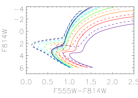
Figure 2.— The age-metallicity degeneracy is shown here with isochrones of different ages covering a range of metallicity: $-2.5<$ [Fe/H] $<+0.5$, black represents the most metal poor, purple the most metal rich, with each color in between representing a 0.5 increment in [Fe/H]; solid lines represent an age of 12.5 Gyr and the dashed lines represent 4 Gyr.
(A color version of this figure is available in the online journal.)

For a population of mixed age, the color-metallicity relation breaks down because younger giants, which are more massive, are hotter than older giants of the same metallicity. The color changes due to age and metallicity are demonstrated in Figure 2, for two different ages (12.5 and 4 Gyr, solid and dashed lines, respectively), and for a range of metallicities (different colors). The effect is quantitatively shown in Figure 3, where color as a function of metallicity is plotted for several ages (2, 7 and 12 Gyr) for a giant branch star with a $M_{F814W}$ = $-1.0$ (with comparable results along the entire giant branch). At higher metallicity this leads to an uncertainty in derived metallicity of a few tenths of a dex, but the uncertainty can be significantly larger at lower metallicity. The uncertainties in metallicity also become greater with younger populations; as Figure 3 shows, the color difference between 2 and 7 Gyr is almost double that between 7 and 12 Gyr.

Figure 3.— Shown above are the giant branch (F555W–F814W) colors at fixed magnitude of F814W $=-1$ for populations of different ages (2, 7, and 12 Gyr) as a function of metallicity. This plot quantitatively demonstrates that small relative changes of color at low metallicity can lead to large changes in metallicity, and the effect is larger in older populations.

2.3. Separating atmospheric parameters using photometric colors

The key to breaking the age-metallicity degeneracy is separating the color effects of metallicity and temperature. Two color indices have the potential to break the degeneracy because one color can measure a metallicity dependent feature in the spectrum, while the other can control for the temperature. The more the two color’s sensitivities to metallicity and temperature differ, the more effective the color combination will be at measureing metallicity.

We examine the temperature and metallicity sensitivity for all the filter combinations by using Kurucz stellar atmosphere models of metallicity ranging from $-5>$ [Fe/H] $>+1$. We integrate the WFC3 transmission curve for each filter over the synthetic spectra with parameters of typical giant branch stars (log g = 2.5 and T_eff = 4500 K). We compute the color change with temperature ($\Delta$ color/$\Delta$ T_e) and metallicity ($\Delta$ color / $\Delta$ [Fe/H]), at a range of metallicities. The ratio of the two gives the relative sensitivity to temperature and metallicity at equal color difference, where small values of $\Delta$ T_e/$\Delta$ [Fe/H] indicate a smaller dependence on metallicity than temperature. The relative sensitivity of temperature to metallicity ($\Delta$ T_e/$\Delta$ [Fe/H]) for all colors is plotted in Figure 4. As expected, the colors whose bandpasses contain fewer metal-features (e.g F555W–F814W and F467M–F547M) are the ones that are least sensitive to metallicity.

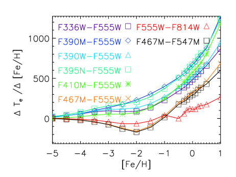
Figure 4.— Relative color change from temperature compared to color change from metallicity, as a function of metallicity, i.e. ($\Delta$ color / $\Delta$ [Fe/H]) / ($\Delta$ color/$\Delta$ T_e) ), measured from Kurucz atmospheric models. (A color version of this figure is available in the online journal.)

Figure 4 shows that the F467M–F547M and F555W–F814W colors have comparably smaller sensitivities to metallicity. However, the relative color error for F467M–F547M is over 3.5 times larger than F555W–F814W for a fixed exposure time. F555W–F814W stands out as the optimal temperature index, considering minimal metallicity sensitivity and photometric accuracy. While F555W–F814W certainly changes with metallicity (cf. its use as a metallicity indicator in clusters at fixed age as discussed in the previous section) it has the largest relative sensitivity of temperature to metallicity of all the filters compared in this section (see Figure 4).

Figure 5 demonstrates the age independence and metallicity separation of a color-color diagram. The plot includes isochrones of two different ages, 12.5 and 4 Gyr, as solid and dashed lines respectively, for a range of metallicities in steps of 0.5 dex. The solid and dashed lines closely follow each other throughout the color-color diagram. The bifurcation of the isochrones at cooler temperatures (especially seen at higher metallicity with the dashed and solid purple lines) is due to dwarf and giant stars colors showing increased gravity sensitivity at higher metallicity. The gravity sensitivity causes the metallicity-sensitive color of dwarfs to be bluer than giants at the same value of the temperature-sensitive color, however, for targets at a common distance, apparent magnitude can be used to separate the evolutionary stage. Based upon the color sensitivities shown in Figure 4, we selected the more metallicity-sensitive colors to use with the temperature-sensitive color (F555W–F814W) in color-color diagrams.

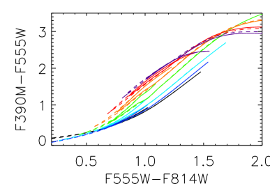
Figure 5.— The color-color diagram breaks the age-metallicity degeneracy. Isochrones cover a range of metallicity: $-2.5<$ [Fe/H] $<+0.5$, the lowest (black) line represents the most metal poor, highest (purple) line the most metal rich, with each line in between representing a 0.5 increment in [Fe/H]; solid lines represent an age of 12.5 Gyr and the dashed lines represent 4 Gyr. (A color version of this figure is available in the online journal.)

Figure 6 shows giant branch isochrones in color-color diagrams for five metallicity sensitive colors: F336W–F555W, F390M–F555W, F390W–F555W, F395N–F555W and F410M–F555W. The effectiveness of these color combinations to determine metallicity are quantified in Table 3 by the color separation due to metallicity predicted from stellar isochrones in color-color diagrams, using units of dex of [Fe/H]/0.01 mag of color change. While all the filter sets have similar sensitivity around solar metallicity ($+0.5>$ [Fe/H] $>-0.5$) this breaks down at lower metallicities.

Table 3Color-Color diagram sensitivity: Metallicity per 0.01 magnitude color change

		Sensitivities
Color	@F555W–	$-4.5<$	$-3.5<$	$-2.5<$	$-1.5<$	$-0.5<$	normalized	[Fe/H] /
	F814W=	[Fe/H]	[Fe/H]	[Fe/H]	[Fe/H]	[Fe/H]	$\sigma_{color}$	(0.01 mag /
		$<-3.5$	$<-2.5$	$<-1.5$	$<-0.5$	$<0.5$		$\sigma_{color}$)
		(dex [Fe/H]/0.01 mag of color change)
F336W–F555W	0.9	0.427	0.143	0.047	0.023	0.026	9.8	0.24
	1.0	0.290	0.107	0.045	0.023	0.024	9.8	0.23
	1.1	0.236	0.087	0.051	0.023	0.024	9.8	0.23
F390W–F555W	0.9	0.943	0.287	0.098	0.041	0.049	1.0	0.04
	1.0	0.704	0.199	0.090	0.038	0.046	1.0	0.04
	1.1	0.541	0.149	0.084	0.038	0.043	1.0	0.04
F390M–F555W	0.9	0.667	0.206	0.074	0.027	0.036	6.9	0.19
	1.0	0.493	0.146	0.062	0.024	0.035	6.9	0.16
	1.1	0.370	0.110	0.052	0.023	0.034	6.9	0.16
F395N–F555W	0.9	0.515	0.151	0.066	0.036	0.049	15.4	0.56
	1.0	0.369	0.104	0.057	0.037	0.047	15.4	0.56
	1.1	0.277	0.079	0.052	0.038	0.047	15.4	0.60
F410M–F555W	0.9	$>$ 1	0.820	0.254	0.090	0.063	2.6	0.23
	1.0	$>$ 1	0.510	0.288	0.070	0.051	2.6	0.16
	1.1	$>$ 1	0.364	0.350	0.063	0.044	2.6	0.16

Note. — Quantified color spans between isochrones 1 dex [Fe/H] apart in the color-color diagrams shown in Figure 6. All numbers are listed in dex of [Fe/H] /0.01 mag of color change. The $\sigma_{color}$ is estimated using the online WFC3 ETC and normalized to $\sigma_{(F390W--F555W)}$. The last column reports the [Fe/H] dex /(0.01 mag/$\sigma$) for the metallicity range $-1.5<$ [Fe/H] $<-0.5$. At extremely low metallicities some of the color changes are beyond typical photometric accuracy, i.e. greater than a dex of color / 0.01 mag of color change.

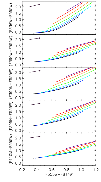
Figure 6.— We show the metallicity sensitivity for different filter combinations using color-color plots of Dartmouth Isochrones above the MSTO. The lines span $-2.5<$ [Fe/H] $<+0.5$, lowest (black) line being the most metal poor, the highest (purple) line the most metal rich. Reddening vectors are indicated with arrows. (A color version of this figure is available in the online journal.)

Weighting the metallicity sensitivity by the relative uncertainty (last column of Table 3) shows that F390W–F555W is the most sensitive for a fixed exposure time. Below [Fe/H] $<-1.5$ the color separation for F395N–F555W, F390M–F555W and F336W–F555W are the most sensitive to metallicity. Although the F395N–F555W color retains sensitivity it also requires 2 to 3 times more exposure time to get comparable accuracy, making it prohibitive to use. At extremely low metallicity the most sensitive color is F395N–F555W, with sensitivity decreasing respectively for the colors: F336W–F555W, F390M–F555W and F390W–F555W.

Based upon the metallicity sensitivity and photometric efficiency we find that the most promising metallicity indicating filters are the F390W, F390M and F336W filters. In the remainder of the paper we will focus our analysis on these filters.

2.4. Reddening Effects

Reddening adds uncertainty to any photometric metallicity derivation, especially when the uncertainty in reddening is large, or if there is differential reddening throughout the field. In a color-color plot uncorrected reddening will be confused with a change in metallicity if the reddening vector is in the direction of the metallicity separation. For the majority of the color-color diagrams the reddening vectors are predominantly in the same direction as the isochrones, mitigating the influence of reddening. However, for (F336W–F555W, F555W–F814W) the reddening vector is $\sim$ 40^∘ shallower than the isochrones, which increases the uncertainty in derived metallicities when there is differential reddening or if the uncertainty in the reddening is large. Reddening vectors are indicated in Figure 6 for E(B–V) = 0.1. The vector is defined by the reddening of the colors along the X and Y axes. For a given color, the reddening E(Filter₁–Filter₂) = $A_{Filter1}-A_{Filter2}$, where A_Filter1 = R_Filter1 E(B–V), and the R_Filter values are listed in Table 1.

To get an estimate of the effect of reddening on metallicities we consider an uncertainty of $\sigma_{E(B-V)}$ = 0.02, as might be appropriate in a low reddening target. At shorter wavelengths, where all of our metallicity sensitive filters are located, the uncertainty in reddening will have an increased effect due to the UV extinction law increasing as wavelength decreases. In this case the $\sigma_{E(B-V)}$ adds a systematic color uncertainty of $\sim$0.1 mag to all of the metallicity sensitive colors. However, the color change from reddening will be along the reddening vector, and because the angles between the isochrones and reddening vectors vary (e.g. Figure 6) and the colors have different sensitivity to metallicity (e.g. Table 3), this leads to metallicity uncertainties ranging from a tenth to a few tenths of a dex. The resulting systematic uncertainties in [Fe/H] are reported in Table 4. As expected, larger uncertainties are found at lower metallicities.

Historically, reddening-free indices have been proposed as a means to correct colors for extinction. A reddening-free index, Q, is defined as:

$$Q=(m_{1}-m_{2})-\frac{E(m_{1}-m_{2})}{E(m_{2}-m_{3})}(m_{2}-m_{3})$$ (1)

where E$(m_{1}-m_{2})$ is the color excess for the color $(m_{1}-m_{2})$ (Johnson & Morgan, 1953). However, making our metallicity indicator reddening-free still leaves the problem that the temperature indicator is affected by reddening. To completely remove reddening effects from the color-color diagram, both indices need to be reddening-free. Brown et al. (2009) suggest using two reddening-free indices (5 total filters, including two in the IR) to predict metallicity. We looked into using these additional filters and found that with our low reddening targets the additional filters do not significantly add to the metallicity resolution.

Table 4Metallicity errors from Reddening

	Metallicity Errors
Color	-2.5 $<$	-1.5 $<$	-0.5 $<$
	[Fe/H]	[Fe/H]	[Fe/H]
	$<$ -1.5	$<$ -0.5	$<$ 0.5
F336W–F555W	0.30	0.14	0.15
F390M–F555W	0.20	0.09	0.13
F390W–F555W	0.23	0.11	0.12
F395N–F555W	0.10	0.07	0.09
F410M–F555W	0.33	0.12	0.08

Note. — Metallicity uncertainties for each color is based on the metallicity sensitivity, the angle between the reddening vector and isochrone sequence, and $\sigma_{\rm{E(B-V)}}=\pm$ 0.02.

2.5. Abundance Ratio Variations

While [Fe/H] is commonly used as a proxy for the overall stellar metallicity, elements do not vary in lockstep from star to star. Variations in abundance ratios can alter spectral features within a bandpass, changing the stellar color and causing the overall photometric metallicity to be misinterpreted if fixed abundance ratios are assumed.

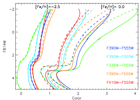
Figure 7.— Color changes due to shifts in $\alpha$ at a low and high metallicity, for 5 metallicity-sensitive colors listed. Solid and dashed lines represent [$\alpha$/Fe] = $+0.4$ and 0.0, at [Fe/H] = $-2.5$, and [$\alpha$/Fe] = $+0.2$ and $-0.2$ at [Fe/H] $=0.0$.
(A color version of this figure is available in the online journal.)

A common abundance variation is $\alpha$ element enhancement (e.g. Ne, Mg, Si, S, Ar, Ca, and Ti), often present at low metallicity in globular clusters (see Tolstoy et al. (2009); McWilliam (2010) and references there in). The CMD of an $\alpha$-enhanced population resembles a CMD of higher [Fe/H] with solar abundance ratios. Figure 7 shows how $\alpha$ enhancements affect different colors at low and high metallicity. Different combinations of [Fe/H] and [$\alpha$/Fe] can give the same colors.

Using Dartmouth isochrones, we compute the relative color change from $\alpha$ abundances ($\Delta$ color/ $\Delta$ [$\alpha$/Fe]) and metallicity ($\Delta$ color/ $\Delta$ [Fe/H]), to find the relative sensitivity of various colors to [Fe/H] and $\alpha$ enhancement. The ratio of the two as a function of metallicity is presented in Table 5; unsurprisingly the colors with the most $\alpha$ sensitivity are the the two colors (F395N–F555W and F390M–F555W) whose bandpasses are dominated by the Ca H $\&$ K lines.

Metallicities assigned assuming solar abundance ratios can be considered as a metallicity indicator that is a combination of the actual [Fe/H] and [$\alpha$/Fe], following the relation:

$$\textrm{[m/H]}_{phot}=\textrm{[Fe/H]}+\left(\frac{\Delta\textrm{[Fe/H]}}{\Delta[\alpha/\textrm{Fe}]}\right)[\alpha/\textrm{Fe}]$$ (2)

where the amount of relative color change due to $\alpha$ enhancements (listed in Table 5) can be used to get the relation.

The differing sensitivity of ($\Delta$[Fe/H]/$\Delta$[$\alpha$/Fe]) in different colors implies that $\alpha$ abundance can be separated with photometry using similar techniques described in Section 2.3. However, additional colors with differing sensitivities would be necessary to isolate the $\alpha$ abundance, such as F395N–F555W and F410M–F555W or F390M–F555W and F390W–F555W.

We should note that the majority of globular clusters show large star-to-star variations in light elements (Li to Si) (for a review see Gratton et al. 2012, and references therein). Additionally there are cluster-to-cluster abundance variations (Carretta et al., 2009), which also have the potential to affect the stellar colors. VandenBerg et al. (2012) found that abundance enhancements of Mg, Si, and to some extent Ca, will change the color and thus location of the giant branch, while variations in oxygen will affect the height of the subgiant branch and the luminosity of the MS turnoff. Of particular interest in this study, C and N enhancements can affect the stellar colors measured with F390M and F390W, since a few CN and CH bands fall in the same spectral region covered by these filter bandpasses; see Section 2.1 for details. Since we cannot explicitily measure any of these abundance variation in this study due to the limited resolution of photometric metallicities, any such variations could affect the stellar colors and our inferred metallicities.

Table 5Relative sensitivity of [Fe/H] to [$\alpha$/Fe]

	$\Delta$[Fe/H] / $\Delta$ [$\alpha$/Fe]
Color	$-2.5<$	$-1.5<$	$-0.5<$
	[Fe/H]	[Fe/H]	[Fe/H]
	$<-1.5$	$<-0.5$	$<0.5$
F336W–F555W	0.27	0.39	0.64
F390W–F555W	0.22	0.19	0.09
F390M–F555W	0.65	0.37	0.34
F395N–F555W	0.88	0.84	0.79
F410M–F555W	0.09	0.17	-0.09

Note. — The relative sensitivity of metallicity compared to $\alpha$ enhancement

3. Testing the method: Observations of calibration clusters

WFC3 images were obtained of five clusters during cycle 17 as part of the calibration program 11729, (PI Holtzman). Additional images of the five clusters come from the calibration portion of the program 11664 (PI Brown). The five clusters were chosen because they are well studied and span a range of [Fe/H]; 5 of the 6 clusters are discussed by Brown et al. (2005) for ACS calibration.

Table 6Exposure Times

WFC3	Exposure Time (sec)
Filter	M 92	NGC 6752	NGC 104	NGC 5927	NGC 6791
F336W	850, 30	1000, 30	1160, 30	950, 30	800, 30
F390M	1400, 50	1400, 50	1400, 50	1400, 50	1400, 50
F390W	2290, 10	2460, 10	2596, 10	2376, 10	2250, 10
F395N	1930, 90	2100, 90	2240, 90	1015, 90	1850, 90
F410M	1530, 40	1600, 40	1600, 40	1600, 40	1490, 40
F467M	700, 40	800, 40	900, 40	730, 40	700, 40
F547M	445	445	445	445	445
F555W	1360.5	1360.5	1360.48	1381	1360.5
F814W	860.5	1020.5	1160.48	961	810.5
F160W	1245, 8.3	1245, 12.5	1245, 16.7	1245, 12.5	1245, 4.2
F110W	1245, 8.3	1245, 12.5	1245, 16.7	1245, 12.5	1245, 4.2

3.1. The Observations

We present data for four globular clusters, M92 (NGC 6341), NGC 6752, NGC 104 (47 Tuc), NGC 5927, and one open cluster NGC 6791. Exposure times are listed in Table 6, and include short and long exposures to increase the dynamic range of the photometry.

3.2. Photometry

Reduced images were obtained from the HST archive using its on-the-fly processing. A deep image was created by summing all of the exposures in F467M, and stars were identified on this image. For each individual frame, a pixel area correction was applied to account for the modification in fluxes by flat fielding, and an astrometric solution was derived relative to the reference frame. Aperture photometry was done on all of the stars using aperture radii of 0.12, 0.25, 0.375, and 0.5 arcsec. Using this initial aperture photometry and model PSFs calculated using TinyTim, photometry was redone on each individual star after subtracting off all neighbors; this process was iterated twice.

3.3. Cluster parameters

To adopt isochrones for the clusters we search the literature for well established cluster parameters. The distance modulus and the reddening are needed to get the absolute magnitudes of the cluster stars. Additionally we use the age, metallicity, and $\alpha$ enhancement to select isochrones for our study. We have compiled a sampling of the reported cluster parameters, and list the literature values adopted in this study in Table 7.

M92 is the only very metal-poor cluster in our sample. Spectroscopic metallicity measurements include those by Zinn & West (1984), [Fe/H] $=-2.24\pm 0.08$, Carretta & Gratton (1997), [Fe/H] $=-2.16\pm 0.02$, and Kraft & Ivans (2003),$\langle$ [Fe/H]_II$\rangle=-2.38\pm 0.02$ and $\langle$ [Fe/H]_I$\rangle=-2.50\pm 0.12$.. We average the spectroscopic metallicities, and adopt [Fe/H] $=-2.30$. Isochrone studies by VandenBerg & Clem (2003) and di Cecco et al. (2010) both found $\alpha$ enhancements of [$\alpha$/Fe] $=+0.3$, however our isochrone grid is in steps of 0.2, so we adopt [$\alpha$/Fe]$=0.4$. We adopt the age, and reddening found by VandenBerg & Clem (2003), 13.5 Gyr and E(B–V) $=0.023$. After adopting these isochrone parameters we adjust the distance modulus to be fully consistent with our isochrone models, by assuming (m–M)${}_{\rm{V}}=14.60$, which is consistent with the values used by VandenBerg & Clem (2003).

NGC 6752. Gratton et al. (2005) measured spectra of seven stars for an overall metallicity [Fe/H] $=-1.48\pm 0.02$, and [$\alpha$/Fe] $=+0.27$ $\pm$0.01. Carretta et al. (2009) measured [Fe/H] $=-1.555\pm 0.07$ from high resolution spectra of 14 stars, they also measured multiple $\alpha$ elments for an average [$\alpha$/Fe] $=+0.35$. In a previous study, Gratton et al. (2003) found [Fe/H] $=-1.43\pm 0.04$. Other spectroscopic metallicity measurements include those by Zinn & West (1984), [Fe/H] $=-1.54\pm 0.09$, Carretta & Gratton (1997), [Fe/H] $=-1.42\pm 0.08$, Kraft & Ivans (2003), $\langle$ [Fe/H]_II$\rangle=-1.50\pm 0.02$. We average the spectroscopic [Fe/H] and adopt a [Fe/H] $=-1.45$, which is slightly lower than the average but is consistent with the larger [$\alpha$/Fe] adopted to fit our isochrone grid, [$\alpha$/Fe]$=0.4$.

We assume a reddening of E(B–V) $=0.046\pm 0.005$ as measured by Gratton et al. (2005) from 118 stars. We adopt an age of 12.5 Gyr, reported by VandenBerg (2000), and also by Marín-Franch et al. (2009) in a study of comparative ages of globular clusters. From these adopted isochrone prameters we adjust our distance modulus to (m–M)${}_{\rm{V}}=13.20$, which is consistent with the distance to NGC 6752 measured by Renzini et al. (1996) using the white dwarf cooling sequence; (m–M)_V= 13.17.

47 Tuc. Spectroscopic measurement include those by Zinn & West (1984), [Fe/H] $=-0.71\pm 0.08$, Carretta & Gratton (1997) who found [Fe/H] $=-0.70\pm 0.07$, Kraft & Ivans (2003), $\langle$ [Fe/H]_II $\rangle=-0.70\pm 0.05$, Wylie et al. (2006) found [Fe/H] $=-0.60\pm 0.2$ based on seven RGB stars, and Carretta et al. (2009) measured [Fe/H] $=-0.74\pm 0.02$ from the medium resolution spectra of 147 stars and [Fe/H] $=-0.77\pm 0.03$ from the high resolution spectra of 11 stars, and measured an [$\alpha$/Fe]$=0.44$. We average the [Fe/H] adopting values of [Fe/H] $=-0.70$ and [$\alpha$/Fe] = 0.4.

We use the E(B–V) $=0.024$ reported by Gratton et al. (2003). VandenBerg & Clem (2003) found an age of 12 Gyr, Zoccali et al. (2001) derived an age of 12.9 Gyr using diffusive models, which we average for an adopted age of 12.5 Gyr. Based upon the adopted isochrone parameters we adjust the distance modulus to (m–M)${}_{\rm{V}}=13.20$ which is smaller than the values measured by Woodley et al. (2012) and Zoccali et al. (2001) who both measured the distance modulus (13.36 and 13.27, respectively) to 47 Tuc using white dwarf cooling models.

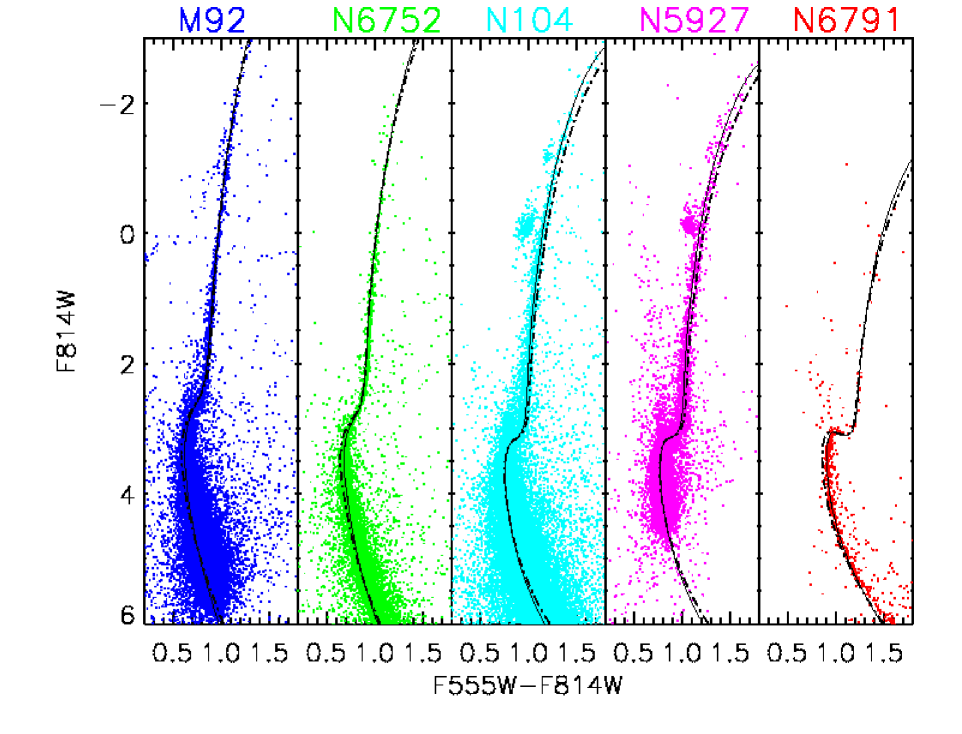
Figure 8.— CMD of (F555W–F814W, F814W), and Dartmouth isochrones of literature value (dashed lines) as listed in Table 7. Empirically corrected isochrones shown as solid lines, corrections listed in Table 8. (A color version of this figure is available in the online journal.)

NGC 5927 is more complicated to study photometrically due to the high differential reddening within the cluster ( $\Delta$ E(V-I)=0.27 measured by Heitsch & Richtler (1999) and $\delta$(E(B–V)=0.169 measured by Bonatto et al. 2013). Zinn & West (1984) found [Fe/H] $=-0.30\pm 0.09$; Armandroff & Zinn (1988) measured [Fe/H] $=-0.31$, while Kraft & Ivans (2003) found [Fe/H] $=-0.67$. We adopt a [Fe/H] of $-0.40$ and [$\alpha$/Fe] of +0.2.

Harris (1996) found the reddening to be E(B–V)= 0.45. De Angeli et al. (2005) did a study on the relative ages of GC’s and found the age to be $\approx$ 10 Gyr, while the relative GC age study by Marín-Franch et al. (2009) determined an age of $\sim$ 11.3 Gyr, we assume an age of 11.5 Gyr. Based upon the adopted isochrone parameters we adjust the distance modulus to (m–M)${}_{\rm{V}}=15.78$.

NGC 6791, unlike the rest of our calibrating clusters, is an open cluster (although recent work by Geisler et al. (2012) suggests that NGC 6791 might be the remains of a stripped globular cluster). Grundahl et al. (2008) determined a metallicity of [Fe/H] $=+0.37$. Origlia et al. (2006) used infrared spectroscopy of 6 stars to measure a [Fe/H] = $+0.35\pm$0.02 and solar $\alpha$ abundance ratio. Chaboyer et al. (1999) found a [Fe/H] $=+0.4$. We average the spectroscopic metallicities and round to the nearest isochrone grid spacing and adopt [Fe/H] $=+0.4$ and [$\alpha$/Fe]=0.0.

We assume the reddening found by Chaboyer et al. (1999), E(B–V) = 0.10${}^{+0.03}_{-0.02}$. We use the age found by both Chaboyer et al. (1999) and Carraro et al. (2006) of 8 Gyr. Brogaard et al. (2012) found an age of $\sim$8.3 Gyr, and García-Berro et al. (2013) also reported a consistent age of 8 Gyr between the white dwarf cooling sequence and the MSTO age. From this we find a distance modulus of (m–M)${}_{\rm{V}}=13.45$, which is consisten with Grundahl et al. (2008) who used an eclipsing binary to determine (m–M)_V = 13.46$\pm$ 0.1, and with Chaboyer et al. (1999), who found (m–M)${}_{\rm{v}}=13.45^{+0.03}_{-0.12}$.

As previously stated the adopted [Fe/H] and [$\alpha$/Fe] are not perfectly matched to the literature values but are rounded to the spacing within the isochrone grid (in steps of 0.05 of [Fe/H] and 0.2 of [$\alpha$/Fe]). When adjusting the metallicity to our grid we note that the [Fe/H] adjustment for a change in [$\alpha$/Fe] varied for each color according to equation (2) and Table 5; therefore we made an average metallicity adjustment that best fit all colors simultaneously.

Table 7Cluster data

Cluster	RA	Dec	E(B–V)	(m–M)v	[Fe/H]	[$\alpha$/Fe]	Age
M 92	17 17 07.05	+43 07 58.2	0.023	14.60	–2.50, –2.14 (–2.30)	+0.30 (+0.4)	13.5
NGC 6752	19 10 54.86	–59 59 11.2	0.046	13.20	–1.54, –1.43 (–1.45)	+0.27 (+0.4)	12.5
NGC 104	00 24 15.26	–72 05 47.9	0.024	13.20	–0.77, –0.60 (–0.70)	+0.44 (+0.4)	12.5
NGC 5927	15 28 00.20	–50 40 26.2	0.45	15.78	–0.67, –0.30 (–0.40)	. . . (+0.2)	11.5
NGC 6791	19 20 53.00	+37 46 30.0	0.10	13.45	+0.35, 0.40 ($+0.40$)	0.0 ( 0.0)	8.0

Note. — The cluster parameters adopted for this study including the reddening, metallicity, and ages from peer reviewed sources discussed and cited in section 3.3. The distance moduli adopted for this study were adjusted to self consistently fit the MSTO and subgiant branchs for each cluster to the adopted isochrones. See Section 3.3 for more details.

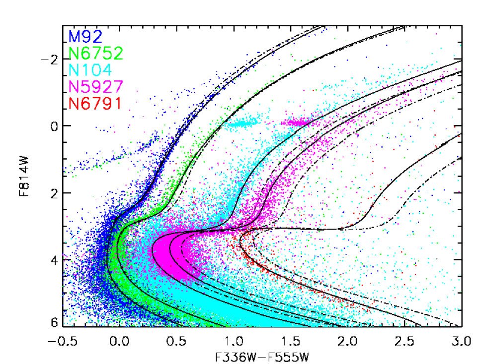
Figure 9.— CMD of (F336W–F555W, F814W) and Dartmouth isochrones of literature value (dashed lines) as listed in Table 7. Empirically corrected isochrones shown as solid lines, corrections listed in Table 8. (A color version of this figure is available in the online journal.)

3.4. Absolute Magnitudes

From the reported reddening, and distance modulus we calculate the Absolute magnitudes for each filter. All magnitudes reported are in the Vegamag system with zeropoints taken from the WFC3 handbook. The absolute magnitudes for each filter were calculated using: M${}_{(filter)}=$ m_observed - ((m–M)_v - A_v) - A_filter. The distance modulus, (m–M)_v, as reported in Table 7, was corrected for the V band extinction, $A_{\rm{v}}$ = 3.1E(B–V), and addtionally corrected for the extinction within the given filter A_(filter) = R_(filter)E(B–V). The ratio of total to selective extinction, R_(filter) as listed in Table 1, was calculated by taking the integral over the stellar atmosphere SED convolved with the filter transmission curve, divided by the integral over the same atmosphere and filter convolved with the galactic extinction curve. We used an atmosphere with [Fe/H] $=-1.5$, temperature of 5000, and log g = 2.0.

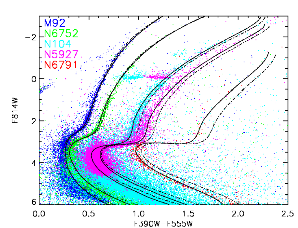
Figure 10.— CMD of F390W–F555W vs. F814W,and Dartmouth isochrones of literature value (dashed lines) as listed in Table 7. Empirically corrected isochrones shown as solid lines, corrections listed in Table 8. (A color version of this figure is available in the online journal.)

4. Cluster Isochrone comparison

It is well known that theoretical isochrone models do not perfectly match observed colors due to a combination of uncertainties from stellar evolution models, model atmospheres, and instrumental systematics. When comparing the isochrone of the mean spectroscopic value to the CMDs the models often did not match the shape of the cluster ridgelines. However, it should be noted that uncertainties in distance, age, reddening and composition complicate the fitting process. The cluster CMDs are shown in Figures 8 - 11, where dashed lines represent the literature valued isochrones adopted for each cluster as reported in Table 7.

In order to improve the metallicity determinations we derived an empirical correction to the isochrones using the five cluster CMDs as benchmarks. For small steps in magnitude along the giant branch, we found the distance between the theoretical isochrone colors and the cluster ridgeline, then squared and summed the distances. Using the canonical metallicities we found the empirical corrections with the smallest summed distance between the corrected isochrone and the cluster. These corrections lead to consistent cluster metallicities across all CMDs. All isochrone corrections were based on color, gravity and metallicity adjustments. The various filter combinations require different functional forms of the generic equation:

Equation (3) was modifed by inspection of the various CMDs. The (F555W–F814W, F814W) CMD in Figure 8 shows the uncorrected literature valued isochrones falling redward of the cluster ridgelines to varying degrees depending on the magnitude and metallicity of the isochrone. The most metal-poor cluster was especially discrepant, with larger deviations along the lower giant branch than the upper. For this CMD the first order color correction includes a dependence on metallicity, which allows for larger corrections at lower metallicity. The first order color dependent term shifts and changes the shape of the isochrone, while the second order metallicity dependent term adds the same shift to a given isochrone without changing the shape. The additional gravity dependent term corrects the bend of the giant branch (where log g $<$ 3.4), with more bend required as metallicity decreases.

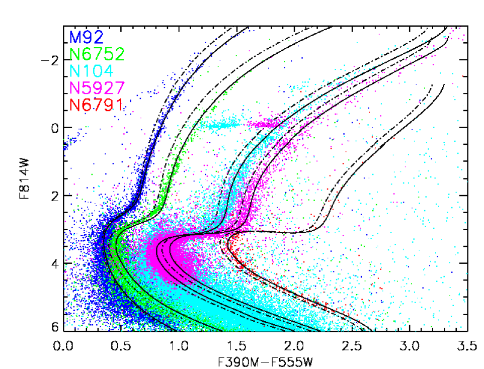
Figure 11.— CMD of (F390M–F555W, F814W), and Dartmouth isochrones of literature value (dashed lines) as listed in Table 7. Empirically corrected isochrones shown as solid lines, corrections listed in Table 8. (A color version of this figure is available in the online journal.)

In Figure 9 the (F336W–F555W, F814W) CMD shows the uncorrected isochrones redward of the cluster ridgelines, except for M92 where the isochrone along the giant branch falls blueward. This CMDs shows the largest difference between the clusters and the models. The bend of the isochrone along the giant branch (where log g $<$ 3.4) is corrected with a gravity and metallicity dependent term, with increasing tilt as metallicity decreases. In this CMD the corrected isochrone for 47 Tuc (NGC 104) falls $\sim$0.03 mag redward of the cluster ridgeline, while all of the other clusters are within $\sim$0.01 mag of their ridgelines. We believe this slight offset to be an artifact of rounding the average spectroscopic metallicity to fit the grid spacing. This color offset is smaller than the color difference between a isochrones of [Fe/H] $=-0.70$ and$-0.75$, therefore we do not force and overcorrection which would potentially lead to distorted MDFs.

In Figure 10 the uncorrected isochrones in the (F390W–F555W, F814W) CMDs are the least discrepant of the CMDs we examined. However a few corrections are still needed to improve the fits, including a metallicity dependent gravity term, with smaller corrections required for lower metallicities.

Table 9Cluster MDF Parameters from CMD fitting

CMD	Cluster	Peak	$\sigma$	$\#$ of
		[Fe/H]		stars
(F336W–F555W, F814W)	M92	-2.28	0.114	937
. . . . . . . . . . . . . . . .	N6752	-1.45	0.073	481
. . . . . . . . . . . . . . . .	N104	-0.74	0.059	2096
. . . . . . . . . . . . . . . .	N5927	-0.37	0.067	1518
. . . . . . . . . . . . . . . .	N6791	0.39	0.079	320
(F390M–F555W, F814W)	M92	-2.32	0.089	899
. . . . . . . . . . . . . . . .	N6752	-1.43	0.087	468
. . . . . . . . . . . . . . . .	N104	-0.68	0.066	2071
. . . . . . . . . . . . . . . .	N5927	-0.42	0.108	1504
. . . . . . . . . . . . . . . .	N6791	0.40	0.098	311
(F390W–F555W, F814W)	M92	-2.33	0.092	906
. . . . . . . . . . . . . . . .	N6752	-1.39	0.060	462
. . . . . . . . . . . . . . . .	N104	-0.66	0.060	2067
. . . . . . . . . . . . . . . .	N5927	-0.46	0.124	1443
. . . . . . . . . . . . . . . .	N6791	0.39	0.082	297

Note. —

The (F390M–F555W, F814W) CMDs presented in Figure 11 shows the uncorrected isochrones blueward of the clusters. Additionally the isochrone curve along the giant branch is too steep to match the shape of the clusters. We applied a first order color term that has an additional metallicity dependence, making the color coefficient greater for lower metallicities.

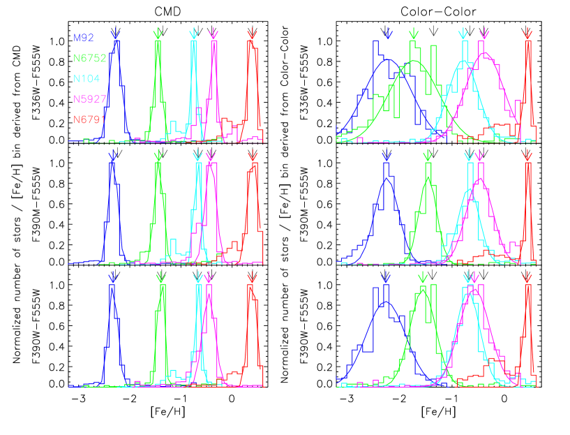
Figure 12.— The MDFs for M92, NGC 6752, NGC 104, NGC 5927 and NGC 6791 (from left to right in each panel) as measured from CMDs and color-color diagrams. The left panels show the normalized distributions of metallicities measured by matching corrected isochrones to stellar colors from CMDs of F336W-F555W, F390M–F555W and F390W–F555W vs. F814W respectively. The right panels show the metallicities measured using corrected isochrones in color-color diagrams of the same colors vs. F555W–F814W. Colored arrows indicate the mean of the distribution, black arrows indicate the metallicities from literature listed in Table 7 with the [Fe/H] adjusted for the adopted [$\alpha$/Fe] compared to the literature values, adjustments were small $\lesssim$ 0.05 dex. (A color version of this figure is available in the online journal.)

The isochrone corrections for all CMDs are listed in Table 8. Finding a single correction to align all five isochrones to the clusters gives us reasonable confidence to interpolate our corrections. Smoothly changing corrections can be applied to the entire set of isochrones, then fit to an unknown population, although caution must be taken when extending beyond our calibrating clusters, i.e. M92 at [Fe/H] $=-2.3$, and NGC 6791 at [Fe/H] $=+0.40$. For the majority of cluster CMDs the empirical corrections improve the isochrone-ridgeline alignment such that the average difference between the two is $\lesssim$ 0.01 mag along the giant branch. In Figures 8 - 11 the dash-dot lines represent the uncorrected isochrones, while the solid lines are the empirically corrected isochrones.

All the color corrections listed in Table 8 are shown to [Fe/H] $=-2.5$. Below this metallicity we replace all of the metallicity dependent terms with the value of the term when [Fe/H] $=-2.5$ keeping the corrections constant where the color change is small and we are unable to verify the corrections.

4.1. Metallicity Determinations

We tested the empirical isochrone corrections by re-deriving the cluster metallicities. We assign photometric metallicities to stars in the CMDs by searching isochrone grids with spacing in [Fe/H] of 0.05 dex; each star was assigned the metallicity of the closest isochrone. We adopted [$\alpha$/Fe] $=0.0$ since we cannot separate the color effects due to $\alpha$ and [Fe/H] with only three filters. We selected giant branch stars with errors $<$0.03 mag in all filters.

4.1.1 Metallicities From CMDs

The photometric metallicities adopted from (F336W–F555W, F814W), (F390M–F555W, F814W) and (F390W–F555W, F814W) were used to create MDFs for every cluster, which are shown on the left side of Figure 12. For all the clusters the MDF peaks are within $\pm$ 0.06 dex of the spectroscopically derived values. The recovered peaks, widths and the number of stars measured are listed in Table 9.

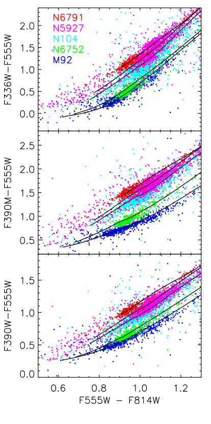
Figure 13.— Shown above are the (F336W–F555W, F555W–F814W), (F390M–F555W, F555W–F814W), and (F390W–F555W, F555W–F814W) color-color diagrams of the five clusters with corrected literature valued isochrones overlaid in black. The corrected isochrones are available in the online version of Table 10. (A color version of this figure is available in the online journal.)

The MDF dispersion within each cluster does not vary much across the metallicity range, although we do see slightly larger numbers for the differentially reddened NGC 5927 and for the lowest metallicity cluster, M92, reflecting the diminished accuracy expected at low metallicity, as discussed in Section 2.2. Additionally for NGC 104 and NGC 5927 the horizontal branch stars are clearly seen as small shoulders left of the MDF peak. The horizontal branch metallicities are systematically lower than the true metallicities because we only use the isochrone colors along the giant branch to assign metallicity, so horizontal branch stars were incorrectly matched to GB stars. Overall, the average MDF dispersion for all clusters is $\sim$0.10 dex and is consistent with what is expected from photometric errors. We simulated this by creating synthetic CMDs based on the IMF and photometric errors within our data set. At each magnitude along the GB ridgeline we used the measured photometric errors to randomly distribute the relative number of stars found at each magnitude. The synthetic CMD was then put through the same isochrone matching processes to get photometric metallicities and a MDF for each cluster.

In order to determine the systematic effect of using uncorrected isochrones to assign photometric metallicities we compared the spectroscopically determined metallicities to those adopted using the uncorrected isochrone grid to assign metallicities. Consistent cluster metallicities could not be found across the various CMDs. For a given CMD the peak of the metallicity distribution varied by $\pm$ 0.4 dex from the canonical values, with the larger discrepancies occurring at low metallicity.

Table 10Corrected isochrone sequence in Color-Color Diagrams

[Fe/H]	(F555W–	(F336W–	(F390M–	(F390W–
	F814W)	F555W)	F555W)	F555W)
-2.30	0.6208	-0.0853	0.3473	0.2647
-2.30	0.6212	-0.0839	0.3476	0.2651
-2.30	0.6217	-0.0825	0.3480	0.2657
. . . .	. . . .	. . . .	. . . .	. . . .
-1.45	0.6804	-0.0160	0.4533	0.3075
-1.45	0.6807	-0.0149	0.4534	0.3077
-1.45	0.6809	-0.0137	0.4536	0.3080
. . . .	. . . .	. . . .	. . . .	. . . .
-0.70	0.7542	0.3142	0.8049	0.5268
-0.70	0.7545	0.3152	0.8052	0.5270
-0.70	0.7550	0.3165	0.8058	0.5276
. . . .	. . . .	. . . .	. . . .	. . . .
-0.40	0.7740	0.4647	0.9201	0.6125
-0.40	0.7743	0.4656	0.9203	0.6129
-0.40	0.7746	0.4668	0.9209	0.6133
. . . .	. . . .	. . . .	. . . .	. . . .
+0.40	0.9087	1.0424	1.4213	0.9728
+0.40	0.9089	1.0435	1.4217	0.9731
+0.40	0.9094	1.0451	1.4223	0.9737

Note. — Table 10 is published in its entirety in the electronic edition of AJ. A portion is shown here for guidance regarding its form and content.

4.1.2 Metallicities From Color-Color Diagrams

To test our metallicity recovery without using age as a known parameter, we apply the empirical corrections to isochrones in color-color diagrams (Figure 13) then adopt metallicities. For each star we found the closest isochrone in the grid (spaced by 0.05 dex in [Fe/H] with the [$\alpha$/Fe] held constant at solar) and assigned the corresponding metallicity. The corrected fiducial isochrone colors shown as black lines in the color-color diagram of Figure 13 are available in the online version in Table 10. The MDFs derived from color-color diagrams are shown on the right side of Figure 12. The recovered peaks, widths and the number of stars measured are listed in Table 11. We selected the same giant branch stars as before, i.e. stars with photometry better than 0.03 mag in all filters. We exclude poorly fit stars, e.g. stars more than 0.25 mag outside of the color range covered by the isochrone grid. This additional constraint accounts for the varying number of stars measured for different color-color diagrams in the last column of Table 11, though the variation is $\sim 1\%$.

For four of the five clusters, only the giant branch stars are used to adopt metallicities in the color-color plots. For the fifth cluster, NGC 6791, there are not enough prominent giant branch stars, necessitating that we additionally use the sub-giant branch and main sequence stars. Theoretically the different evolutionary states should not affect the metallicity determination because we selected the corresponding portion of the isochrone to match the less evolved stars.

The MDFs from color-color diagrams, as compared to those from CMDs, tend to have slightly larger offsets from the spectroscopically derived values, and systematically larger MDF dispersions. However, these metallicities were adopted without any age information, which is necessary for measuring metallicities for a population of mixed ages. The MDFs from the (F390M–F555W) color-color diagrams have mean metallicities within $\pm$ 0.07 dex for all clusters. The MDFs from the (F390W–F555W) color-color diagrams produces mean metallicities within $\pm$ 0.05 dex for M92, NGC 104 (47Tuc) and NGC 6791, and peaks within $\sim$ 0.2 dex for NGC 6752 and the differentially reddened NGC 5927. The MDFs from the (F336W–F555W) color-color diagram finds mean metallicities of $\sim$0.05 dex for most clusters, with the exception of NGC 104 which is discrepant by 0.1 dex.

The larger MDF widths from the color-color diagrams as opposed to the CMD are a natural consequence of using color on the y-axis as opposed to magnitude. The change in color for the total range in metallicity is generally smaller than that for magnitude (see Section 2), thus there is decreased resolution when using color-color diagrams; additionally, the errors for colors are larger than for magnitudes. Together, the decreased color span and the increased errors both add to the uncertainty in the photometric metallicities adopted from color-color diagrams widening the MDFs. The derived MDF widths are consistent with what is expected based upon the photometric errors.

Table 11Cluster MDF Parameters from CC diagrams

Color Color	Cluster	Peak	$\sigma$	$\#$ of
Diagram		[Fe/H]		stars
(F336W–F555W,	M92	-2.22	0.471	879
F555W–F814W)	N6752	-1.73	0.484	454
. . . . . . . . . .	N104	-0.79	0.285	2067
. . . . . . . . . .	N5927	-0.38	0.365	1147
. . . . . . . . . .	N6791	0.37	0.075	320
(F390M–F555W,	M92	-2.25	0.244	906
F555W–F814W)	N6752	-1.46	0.172	448
. . . . . . . . . .	N104	-0.68	0.201	2110
. . . . . . . . . .	N5927	-0.47	0.264	1322
. . . . . . . . . .	N6791	0.37	0.061	314
(F390W–F555W,	M92	-2.27	0.396	891
F555W–F814W)	N6752	-1.57	0.250	447
. . . . . . . . . .	N104	-0.70	0.232	2107
. . . . . . . . . .	N5927	-0.58	0.296	1298
. . . . . . . . . .	N6791	0.36	0.073	303

Of the three color-color diagrams tested to assign metallicity the (F336W–F555W, F555W–F814W) diagram does the worst. For NGC 104 the peak metallicity is off by 0.09 dex and the MDF dispersions are twice to three times the dispersions from (F390M–F555W, F555W–F814W) depending on the cluster. F336W, while predicted to remain sensitive at low metallicity, does not show this in practice, as seen from the wide dispersions for the clusters. The overestimate of the sensitivity could be due to the fact that the color separation, as seen from the clusters, is smaller than predicted from the isochrones, both of which are shown in Figure 9.

The (F390M–F555W, F555W–F814W) color-color diagram generally does the best job deriving metallicities of all the colors. The MDFs have peaks within $\pm$ 0.07 dex of the spectroscopically determined metallicities for all clusters. The MDF dispersions are $\lesssim$ 0.2 dex, except for the very-low metallicity M92 at 0.24 dex and the differentially reddened NGC 5927 at 0.26 dex. The MDFs derived using the (F390M–F555W) color are better than those from (F390W–F555W) and (F336W–F555W). In particular the MDF dispersion in the very-metal poor regime is the narrowest of all the MDFs from color-color diagrams by almost a factor of two. The greater accuracy in photometric metallicities below [Fe/H] $<-1.0$ when using the F390M makes this filter the most useful when working in the very-low metallicity regime.

The (F390W–F555W, F555W–F814W) color-color diagram recovers peaks within $\pm$ 0.2 dex of the spectroscopically determined metallicities. The MDF dispersions are $\sim$ 0.25 dex, except for M92, the very-low metallicity cluster, where the dispersion is 0.4 dex. However, F390W is very economical in terms of integration time, and accurate to $\sim$0.25 dex above [Fe/H] $>-2.0$, therefore this filter is most useful when working in the more metal rich regimes.

In order to determine the systematic effect of using uncorrected isochrones to assign photometric metallicities we compared the spectroscopically determined metallicities to those adopted using the uncorrected isochrone grid in color-color diagrams to assign metallicities. In the MDFs from the color-color diagrams of (F336W–F555W, F555W–F814W) and (F390W–F555W, F555W–F814W) the adopted cluster metallicities were within $\sim$0.2 dex of the spectroscopically derived values for the clusters with metallicities between $-1.5<$ [Fe/H] $<0$, while the very metal poor and metal rich cluster are 3 to 4 times more discrepant. In the color-color diagram of (F390M–F555W, F555W–F814W) the metallicities are all systematically higher by 0.4 to 0.8 dex, again, with more disparate values for very metal poor and metal rich clusters.

5. Conclusion

We explored the metallicity and temperature sensitivities of colors created from nine WFC3/UVIS filters aboard the HST using Dartmouth isochrones and Kurucz atmospheres models. The theoretical isochrone colors were tested and calibrated against observations of five well studied clusters.

We found that (F390W–F555W), and (F390M–F555W), are the most promising colors in terms of metallicity sensitivity. For almost all of the clusters F390M has slightly better metallicity sensitivity, and narrower MDF dispersions, although the F390W filter requires much less integration time. Additionally, at low metallicity the photometric metallicities from (F390M–F555W) are nearly twice as accurate as those from (F390W–F555W).

Using photometry of M92, NGC 6752, NGC 104, NGC 5927 and NGC 6791, all of which have spectroscopically determined metallicities spanning $-2.30<$ [Fe/H] $<+0.4$, we found empirical corrections to the Dartmouth isochrone grid for each of the following CMDs (F555W–F814W, F814W), (F336W–F555W, F814W), (F390M–F555W, F814W) and (F390W–F555W, F814W).

Using the empirical corrections we tested the accuracy and spread of the photometric metallicities adopted from CMDs and color-color diagrams. From the color-color diagrams we were able to recover the spectroscopic metallicities independent from any assumptions about cluster ages, which allows us to apply the color-color diagram method of determining metallicities to complex stellar populations with confidence that the method breaks the age-metallicity degeneracy.

When using color-color diagrams to assign metallicity, we found the (F390M–F555W) color to have the greatest accuracy and consistency across the entire metallicity range, with the main advantage being the increased sensitivity at low metallicity, while (F336W–F555W) and (F390W–F555W) both lose accuracy in this range. We showed that by using the calibrated isochrones we could assign the overall cluster metallicity to within $\sim$ 0.1 dex in [Fe/H] when using CMDs (i.e when the distance, reddening and ages are approximately known). The measured MDFs from color-color diagrams show this method measures metallicities of stellar clusters of unknown age and metallicity with an accuracy of $\sim$ 0.2 - 0.58 dex using F336W, $\sim$0.15 - 0.3 dex using F390M, and $\sim$0.2 - 0.52 dex with F390W, with the larger uncertainty pertaining to lowest metallicity range.

6. Acknowledgements

Support for program 11729 was provided by NASA through a grant from the Space Telescope Science Institute, which is operated by the Association of Universities for Research in Astronomy, Inc., under NASA contract NAS 5-26555.

Table 8Empirical corrections for isochrone colors

Correction	Conditions
$\rm{(F555W-F814W)}_{n}=(0.89+0.028\rm{\textrm{[Fe/H]}})\rm{(F555W-F814W)}_{o}+0.136$	log g $>$ 3.4, $\&$ -2.5 $\leq$ [Fe/H]$<$ -1.4
$\rm{(F555W-F814W)}_{n}=(0.89+0.028\rm{\textrm{[Fe/H]}})\rm{(F555W-F814W)}_{o}+0.136-(0.015\rm{\textrm{[Fe/H]}})(3.4-\log{g})$	log g $<$ 3.4, $\&$ -2.5 $\leq$ [Fe/H]$<$ -1.4
$\rm{(F555W-F814W)}_{n}=(0.89+0.028\rm{\textrm{[Fe/H]}})\rm{(F555W-F814W)}_{o}+0.05(\rm{\textrm{[Fe/H]}}+0.55)^{2}+0.10$	log g $>$ 3.4, $\&$ -1.4 $\leq$ [Fe/H]$<$ 0.5
$\rm{(F555W-F814W)}_{n}=(0.89+0.028\rm{\textrm{[Fe/H]}})\rm{(F555W-F814W)}_{o}+0.05(\rm{\textrm{[Fe/H]}}+0.55)^{2}+0.10-(0.015\rm{\textrm{[Fe/H]}})(3.4-\log{g})$	log g $<$ 3.4, $\&$ -1.4 $\leq$ [Fe/H]$<$ 0.5
$\rm{(F336W-F555W)}_{n}=0.88\rm{(F336W-F555W)}_{o}-0.009$	log g $>$ 3.4, $\&$ -2.5 $<$ [Fe/H]$\leq$ -1.65
$\rm{(F336W-F555W)}_{n}=0.88\rm{(F336W-F555W)}_{o}-0.009+(0.015-0.036\rm{\textrm{[Fe/H]}})(3.4-\log{g})$	log g $<$ 3.4, $\&$ -2.5 $<$ [Fe/H]$\leq$ -1.65
$\rm{(F336W-F555W)}_{n}=0.88\rm{(F336W-F555W)}_{o}+0.04(\rm{\textrm{[Fe/H]}}+0.80)^{2}-0.02$	log g $>$ 3.4, $\&$ -1.65$<$[Fe/H] $\leq$ 0.05
$\rm{(F336W-F555W)}_{n}=0.88\rm{(F336W-F555W)}_{o}+0.04(\rm{\textrm{[Fe/H]}}+0.80)^{2}-0.02+(0.015-0.036\rm{\textrm{[Fe/H]}}(3.4-\log{g})$	log g $<$ 3.4, $\&$ -1.65$<$[Fe/H] $\leq$ 0.05
$\rm{(F336W-F555W)}_{n}=0.88\rm{(F336W-F555W)}_{o}-0.009$	log g $>$ 3.4, $\&$ 0.05$<$[Fe/H] $\leq$ 0.5
$\rm{(F336W-F555W)}_{n}=0.88\rm{(F336W-F555W)}_{o}-0.009+(0.015-0.036\rm{\textrm{[Fe/H]}})(3.4-\log{g})$	log g $<$ 3.4, $\&$ 0.05$<$[Fe/H] $\leq$ 0.5
$\rm{(F390W-F555W)}_{n}=(0.89+0.012\rm{\textrm{[Fe/H]}})\rm{(F390W-F555W)}_{o}+0.01(\rm{\textrm{[Fe/H]}}+2.5)^{2}+0.05$	log g $>$ 3.3, $\&$ -2.5 $<$ [Fe/H] $<$ 1.65
$\rm{(F390W-F555W)}_{n}=(0.89+0.012\rm{\textrm{[Fe/H]}})\rm{(F390W-F555W)}_{o}+0.01(\rm{\textrm{[Fe/H]}}+2.5)^{2}+0.05+(0.07+0.006\rm{\textrm{[Fe/H]}})(3.3-\log{g})$	log g $<$ 3.3, $\&$ -2.5 $<$ [Fe/H] $<$ 1.65
$\rm{(F390W-F555W)}_{n}=(0.89+0.012\rm{\textrm{[Fe/H]}})\rm{(F390W-F555W)}_{o}+0.057$	log g $>$ 3.3, $\&$ -1.65 $<$ [Fe/H] $<$ +0.5
$\rm{(F390W-F555W)}_{n}=(0.89+0.012\rm{\textrm{[Fe/H]}})\rm{(F390W-F555W)}_{o}+0.057+(0.07+0.006\rm{\textrm{[Fe/H]}})(3.3-\log{g})$	log g $<$ 3.3, $\&$ -1.65 $<$ [Fe/H] $<$ 0.5
$\rm{(F390M-F555W)}_{n}=(1.01-0.005\rm{\textrm{[Fe/H]}})\rm{(F390M-F555W)}_{o}+0.07(\rm{\textrm{[Fe/H]}}+2.50)^{2}+0.005$	log g $>$ 3.2, $\&$ -2.5 $<$ [Fe/H]$<$ -1.65
$\rm{(F390M-F555W)}_{n}=(1.01-0.005\rm{\textrm{[Fe/H]}})\rm{(F390M-F555W)}_{o}+0.07(\rm{\textrm{[Fe/H]}}+2.50)^{2}+0.005+(0.018-0.011\rm{\textrm{[Fe/H]}})(3.2-\log{g})$	log g $<$ 3.2, $\&$ -2.5 $<$ [Fe/H]$<$ -1.65
$\rm{(F390M-F555W)}_{n}=(1.01-0.005\rm{\textrm{[Fe/H]}})\rm{(F390M-F555W)}_{o}+0.056$	log g $>$ 3.2, $\&$ -1.65 $<$ [Fe/H]$<$ +0.5
$\rm{(F390M-F555W)}_{n}=(1.01-0.005\rm{\textrm{[Fe/H]}})\rm{(F390M-F555W)}_{o}+0.056+(0.018-0.011\rm{\textrm{[Fe/H]}})(3.2-\log{g})$	log g $<$ 3.2, $\&$ -1.65 $<$ [Fe/H]$<$+0.5

Note. — Derived isochrone corrections.

References

- Anthony-Twarog et al. (1991) Anthony-Twarog, B. J., Twarog, B. A., Laird, J. B., & Payne, D. 1991, AJ, 101, 1902
- Armandroff & Zinn (1988) Armandroff, T. E., & Zinn, R. 1988, AJ, 96, 92
- Bonatto et al. (2013) Bonatto, C., Campos, F., & Kepler, S. O. 2013, Mem. Soc. Astron. Italiana, 84, 187
- Brogaard et al. (2012) Brogaard, K., VandenBerg, D. A., Bruntt, H., et al. 2012, A&A, 543, A106
- Brown (2008) Brown, T. 2008, in HST Proposal, 11664
- Brown et al. (2005) Brown, T. M., Ferguson, H. C., Smith, E., et al. 2005, AJ, 130, 1693
- Brown et al. (2009) Brown, T. M., Sahu, K., Zoccali, M., et al. 2009, AJ, 137, 3172
- Calamida et al. (2007) Calamida, A., Bono, G., Stetson, P. B., et al. 2007, ApJ, 670, 400
- Canterna (1976) Canterna, R. 1976, AJ, 81, 228
- Carraro et al. (2006) Carraro, G., Villanova, S., Demarque, P., et al. 2006, ApJ, 643, 1151
- Carretta et al. (2009) Carretta, E., Bragaglia, A., Gratton, R., D’Orazi, V., & Lucatello, S. 2009, A&A, 508, 695
- Carretta & Gratton (1997) Carretta, E., & Gratton, R. G. 1997, A&AS, 121, 95
- Castelli & Kurucz (2004) Castelli, F., & Kurucz, R. L. 2004, ArXiv Astrophysics e-prints
- Chaboyer et al. (1999) Chaboyer, B., Green, E. M., & Liebert, J. 1999, AJ, 117, 1360
- Da Costa & Armandroff (1990) Da Costa, G. S., & Armandroff, T. E. 1990, AJ, 100, 162
- Da Costa et al. (2002) Da Costa, G. S., Armandroff, T. E., & Caldwell, N. 2002, AJ, 124, 332
- Da Costa et al. (2000) Da Costa, G. S., Armandroff, T. E., Caldwell, N., & Seitzer, P. 2000, AJ, 119, 705
- De Angeli et al. (2005) De Angeli, F., Piotto, G., Cassisi, S., et al. 2005, AJ, 130, 116
- di Cecco et al. (2010) di Cecco, A., Becucci, R., Bono, G., et al. 2010, PASP, 122, 991
- Dotter et al. (2008) Dotter, A., Chaboyer, B., Jevremović, D., et al. 2008, ApJS, 178, 89
- Gallart (2008) Gallart, C. 2008, in Astronomical Society of the Pacific Conference Series, Vol. 390, Pathways Through an Eclectic Universe, ed. J. H. Knapen, T. J. Mahoney, & A. Vazdekis, 278
- García-Berro et al. (2013) García-Berro, E., Torres, S., Isern, J., et al. 2013, in European Physical Journal Web of Conferences, Vol. 43, European Physical Journal Web of Conferences, 5003
- Geisler et al. (2012) Geisler, D., Villanova, S., Carraro, G., et al. 2012, ArXiv e-prints
- Gratton et al. (2003) Gratton, R. G., Bragaglia, A., Carretta, E., et al. 2003, A&A, 408, 529
- Gratton et al. (2005) —. 2005, A&A, 440, 901
- Gratton et al. (2012) Gratton, R. G., Carretta, E., & Bragaglia, A. 2012, A&A Rev., 20, 50
- Grundahl et al. (2008) Grundahl, F., Clausen, J. V., Hardis, S., & Frandsen, S. 2008, A&A, 492, 171
- Harris (1996) Harris, W. E. 1996, AJ, 112, 1487
- Heitsch & Richtler (1999) Heitsch, F., & Richtler, T. 1999, A&A, 347, 455
- Holtzman (2008) Holtzman, J. 2008, in HST Proposal, 11729
- Holtzman (2009) Holtzman, J. 2009, in HST Proposal, 12304
- Johnson & Morgan (1953) Johnson, H. L., & Morgan, W. W. 1953, ApJ, 117, 313
- Kirby et al. (2011) Kirby, E. N., Lanfranchi, G. A., Simon, J. D., Cohen, J. G., & Guhathakurta, P. 2011, ApJ, 727, 78
- Kraft & Ivans (2003) Kraft, R. P., & Ivans, I. I. 2003, PASP, 115, 143
- Lianou et al. (2011) Lianou, S., Grebel, E. K., & Koch, A. 2011, A&A, 531, A152
- Marín-Franch et al. (2009) Marín-Franch, A., Aparicio, A., Piotto, G., et al. 2009, ApJ, 694, 1498
- McWilliam (2010) McWilliam, A. 2010, in Nuclei in the Cosmos
- Origlia et al. (2006) Origlia, L., Valenti, E., Rich, R. M., & Ferraro, F. R. 2006, ApJ, 646, 499
- Renzini et al. (1996) Renzini, A., Bragaglia, A., Ferraro, F. R., et al. 1996, ApJ, 465, L23
- Saviane et al. (2000) Saviane, I., Rosenberg, A., Piotto, G., & Aparicio, A. 2000, A&A, 355, 966
- Strömgren (1966) Strömgren, B. 1966, ARA&A, 4, 433
- Tolstoy et al. (2009) Tolstoy, E., Hill, V., & Tosi, M. 2009, ARA&A, 47, 371
- VandenBerg (2000) VandenBerg, D. A. 2000, ApJS, 129, 315
- VandenBerg et al. (2012) VandenBerg, D. A., Bergbusch, P. A., Dotter, A., et al. 2012, ApJ, 755, 15
- VandenBerg & Clem (2003) VandenBerg, D. A., & Clem, J. L. 2003, AJ, 126, 778
- Woodley et al. (2012) Woodley, K. A., Goldsbury, R., Kalirai, J. S., et al. 2012, AJ, 143, 50
- Wylie et al. (2006) Wylie, E. C., Cottrell, P. L., Sneden, C. A., & Lattanzio, J. C. 2006, ApJ, 649, 248
- Zinn & West (1984) Zinn, R., & West, M. J. 1984, ApJS, 55, 45
- Zoccali et al. (2001) Zoccali, M., Renzini, A., Ortolani, S., et al. 2001, ApJ, 553, 733