KIAS-P13059
EFI-13-28

Exact Partition Functions on $\mathbb{RP}^{2}$ and Orientifolds

Heeyeon Kim^†, Sungjay Lee^⋄, and Piljin Yi^‡

^†Department of Physics and Astronomy, Seoul National University,
Seoul 151-147, Korea ^⋄Enrico Fermi Institute and Department of Physics University of Chicago
5620 Ellis Av., Chicago Illinois 60637, USA ^‡School of Physics, Korea Institute for Advanced Study, Seoul 130-722, Korea

We consider gauged linear sigma models (GLSM) on $\mathbb{RP}^{2}$, obtained from a parity projection of $S^{2}$. The theories admit squashing deformation, much like GLSM on $S^{2}$, which allows us to interpret the partition function as the overlap amplitude between the vacuum state and crosscap states. From these, we extract the central charge of Orientifold planes, and observe that the Gamma class makes a prominent appearance as in the recent D-brane counterpart. We also repeat the computation for the mirror Landau-Ginzburg theory, which naturally brings out the $\theta$-dependence as a relative sign between two holonomy sectors on $\mathbb{RP}^{2}$. We also show how our results are consistent with known topological properties of D-brane and Orientifold plane world-volumes, and discuss what part of the wrapped D-brane/Orientifold central charge should be attributed to the quantum volumes.

1 Introduction and Summary

The two-dimensional (2,2) gauged linear sigma model (GLSM) is a very useful tool for studying conformal field theories of Calabi-Yau manifolds [1]. It allows us to understand how the large volume limit is smoothly connected to Landau-Ginzburg descriptions, and provides an intuitive and straightforward proof of the mirror symmetry.

The most notable development involving GLSM in recent years, by far, is the formulation of GLSM on $S^{2}$ and on squashed $S^{2}$, and the computation of the partition function thereof. As conjectured initially in Ref. [2] and argued from the squashed $S^{2}$ versions in Ref. [3], this leads to a new way to compute exact geometry of Kähler moduli space, without referring to the mirror symmetry dual. The conjectured relationship to the A-model $tt^{*}$-amplitude with Kähler parameters, or the complexified FI parameters $\tau$, is

$$e^{-{\cal K}(\tau,\bar{\tau})}={}_{R}\langle 0|\bar{0}\rangle_{R}=Z_{S^{2}}(\tau,\bar{\tau})\ ,$$ (1.1)

where ${}_{R}\langle 0|$ is a canonical ground state of the Ramond sector [4], $Z_{S^{2}}$ is a two-sphere partition function of (2,2) GLSM which was calculated exactly using supersymmetric localization at [5, 6]. This provides a direct method of computing Gromov-Witten invariants, i.e., the world-sheet instanton contribution to the above quantity, in a manner that obviates the mirror B-model.

This in turn leads to another natural question of how boundary state amplitudes are computed in this new approach. Refs. [7, 8, 9] extended the above to a hemisphere partition function. Interestingly, the supersymmetry that survives the squashing of $S^{2}$ is such that it is naturally A-twisted (anti-A-twisted) at the poles but at the same time B-twisted at the equator. Thus, the boundary states one can attach to the hemisphere are holomorphic cycles wrapped by D-branes. Along the same logic as above, the hemisphere partition function then computes the overlap amplitude between the canonical vacuum and the boundary states in question,

$$\Pi_{B}^{0}(\tau)={}_{R}\langle 0|B\rangle_{R}=Z_{D^{2}}(B,\tau)\ ,$$ (1.2)

which is nothing but the central charge of the D-brane.

One of more interesting results from this can be seen from the large volume limit. Explicit results for simple hypersurface examples, say that the central charge in the large volume limit is

$$\int_{\cal X}e^{-B-iJ}\wedge ch({\cal F})\wedge\hat{\Gamma}_{c}({\cal T})\ ,$$ (1.3)

where $\hat{\Gamma}_{c}({{\cal T}})$ is a multiplicative characteristic class defined by

$$\hat{\Gamma}_{c}({{\cal T}})=\prod_{i=1}^{d}\Gamma\left(1+\frac{x_{i}}{2\pi i}\right)\ ,$$ (1.4)

and ${\cal T}$ is the (holomorphic) tangent bundle of the Calabi-Yau. Most notably, this corrects the conventional form of the central charge as

$$\sqrt{{\cal A}({\cal T})}\quad\rightarrow\quad\hat{\Gamma}_{c}({{\cal T}})\ .$$ (1.5)

This appearance of $\hat{\Gamma}_{c}$ class has been foretold from various explicit computations via mirror symmetry [10, 11, 12, 13].

In this note, we initiate extending these works to the presence of Orientifold planes. The simplest quantity one can compute is the vacuum-to-crosscap amplitude,

$${}_{R}\langle 0|{{\cal C}}\rangle_{R}\ .$$ (1.6)

Pictorially, this is computed by a cigar-like geometry with the identity operator at the tip and a crosscap at the other end. There are two possible choices for the crosscap, say, A-type and B-type. The former corresponds to Orientifold planes wrapping Lagrange subcycles. In this note, we are led to consider B-type parity for GLSM, for much the same reason as in Ref. [14], which corresponds to Orientifold planes wrapping the holomorphic cycles. Topologically the world-sheet is that of $\mathbb{RP}^{2}$, and the same squashing deformation as in Ref. [3] is allowed, the partition function of GLSM on $S^{2}/Z_{2}=\mathbb{RP}^{2}$ is expected to compute the vacuum-to-crosscap amplitude,

$${}_{R}\langle 0|{\cal C}\rangle_{R}=Z_{\mathbb{RP}^{2}}(O,\tau)\ .$$ (1.7)

In the convention of Brunner-Hori [14], the relevant parity action for our purpose here is of type B, which leads to, generally, holomorphically embedded Orientifold planes. Computation of the partition function follows easily from the $S^{2}$ partition function computation, and the result is expressed in terms of a product of the Gamma functions. See section 3 for the complete expressions.

For Orientifold plane that wraps the Calabi-Yau ${\cal X}$ entirely, we also take the large volume limit of the central charge. Conventionally, Orientifold planes, $O^{\pm}$, have ${\cal L}^{1/2}$ class as the counterpart of D-branes’ ${\cal A}^{1/2}$ class. Here we find that one must also replace

$$\sqrt{{\cal L}({\cal T}/4)}\quad\rightarrow\quad\frac{{\cal A}({\cal T}/2)}{\hat{\Gamma}_{c}(-{\cal T})}\ .$$ (1.8)

The parity action on $S^{2}$ can be augmented by additional $Z_{2}$ action on the chiral fields, which induces various combinations of $O_{2(d-s)}$ planes, say wrapping a submanifold ${\cal M}$. For these cases, we must also replace

$$\sqrt{\frac{{\cal L}({\cal T}/4)}{{\cal L}({\cal N}/4)}}\quad\rightarrow\quad\frac{{\cal A}({\cal T}/2)}{\hat{\Gamma}_{c}(-{\cal T})}\wedge\frac{\hat{\Gamma}_{c}({\cal N})}{{\cal A}({\cal N}/2)}\ ,$$ (1.9)

with the normal bundle ${\cal N}$ and the tangent bundle ${\cal T}$ of holomorphically embedded ${\cal M}$ in the Calabi-Yau ${\cal X}$. For more complete expression for the large volume limit, see section 5.

The results found here should be consistent with the hemisphere computation of the D-brane central charges. Among those issues discussed are anomaly inflow and a twist that is known to be present when the world-volume wraps a Spin^c (rather than Spin, i.e.) submanifold. Also, one outfall from having both D-brane and Orientifold plane central charges available is the interpretation of exactly what the Gamma class corrects. The central charge does not by itself tells us whether the correction goes to the RR-charge or the vacuum expectation values of spacetime scalars, or equivalently the quantum volumes. Our conclusion is that the correction should be attributed entirely to the $\alpha^{\prime}$ correction of volumes.

This note is organized as follows. Section 2 outlines GLSM on $\mathbb{RP}^{2}$ as a type B-parity projection of that on $S^{2}$, and briefly discusses squashing deformation of $\mathbb{RP}^{2}$ to motivate the interpretation of the $\mathbb{RP}^{2}$ partition functions as vacuum-to-crosscap amplitudes. Section 3 computes the partition function exactly: We start with identification of two saddle points, of even and odd holonomy respectively, and compute the relevant 1-loop determinants of chiral and vector multiplets. The parity action can be accompanied by $Z_{2}$ flavor rotations, which correspond to Orientifold planes of even co-dimensions. In section 4, we turn to the mirror Landau-Ginzburg description and recover the results of section 3. Here we also learn how the two possible values of $\theta$ angle, i.e. $\theta=0,\pi$, affect the partition functions and sometimes distinguish the (relative) type of Orientifolds from different holonomy sectors.

Section 5 specializes the result to the case of Calabi-Yau hypersurface ${\cal X}$ in $\mathbb{CP}^{N-1}$, and various Orientifolds thereof, and extracts the perturbative contribution. This gives the large volume expression of the central charge, where the $\hat{\Gamma}_{c}$ class makes appearance as in (1.8) and (1.9). Section 6 will consider subtleties and make some consistency checks, from the simple tadpole condition to anomaly inflow. The latter in particular suggests that topological content of D-branes and Orientifold planes remain unchanged despite the changes in the central charges. We point out that, in all central charge expressions from the hemisphere and $\mathbb{RP}^{2}$ partition functions, the multiplicative shift due to the appearance of $\hat{\Gamma}_{c}$ class must be understood as quantum shift of $e^{-iJ}$, such that the RR-charges and the Chern-Simon couplings remain unchanged.

In the Appendices, we outline some technical aspects of the computation but also address a well-known subtlety when ${\cal M}$ is a proper submanifold of Spin^c structure. Invoking tachyon condensation, we motivate natural R-charge and gauge charge assignment for the boundary Hilbert space, how an extra factor $e^{-c_{1}({\cal N})/2}$ emerges for D-branes when ${\cal M}$ is a proper and Spin^c submanifold.

2 GLSM on $\mathbb{RP}^{2}$ and Squashing

In this section, we start with a brief review on general aspects of parity symmetries in 2d (2,2) theory on $\mathbb{R}^{1+1}$, which were thoroughly studied in Ref. [14]. To begin with, the parity action on the 2-dimensional superspace $(x^{\pm}=x^{0}\pm x^{1},\theta^{\pm},\bar{\theta}^{\pm})$ is $x^{1}\rightarrow-x^{1}$, accompanied by the proper action in the fermionic coordinates. Depending on the latter there are two distinct possibilities,

$$\Omega_{A} : (x^{\pm},\theta^{\pm},\bar{\theta}^{\pm})\rightarrow(x^{\mp},-\bar{\theta}^{\mp},-\theta^{\mp})\ ,$$

$$\Omega_{B} : (x^{\pm},\theta^{\pm},\bar{\theta}^{\pm})\rightarrow(x^{\mp},\theta^{\mp},\bar{\theta}^{\mp})\ ,$$ (2.1)

which we will call A and B-parity respectively. Under this action, the four supercharges transform as

$$A : Q_{\pm}\rightarrow\bar{Q}_{\mp},~{}~{}\bar{Q}_{\pm}\rightarrow Q_{\mp},$$

$$D_{\pm}\rightarrow\bar{D}_{\mp},~{}~{}\bar{D}_{\pm}\rightarrow D_{\mp},$$

$$B : Q_{\pm}\rightarrow Q_{\mp},~{}~{}\bar{Q}_{\pm}\rightarrow\bar{Q}_{\mp},$$ (2.2)

$$D_{\pm}\rightarrow D_{\mp},~{}~{}\bar{D}_{\pm}\rightarrow\bar{D}_{\mp}\ .$$

Hence, under the A-parity action, half of the supersymmetry is broken, leaving $Q_{A}\equiv Q_{+}+\bar{Q}_{-}$ and $Q_{A}^{\dagger}$ invariant. Under B-parity, and $Q_{B}\equiv\bar{Q}_{+}+\bar{Q}_{-}$ and $Q_{B}^{\dagger}$ survive.

Furthermore, the simplest transformation rule for a chiral field $(\phi,\psi,F)$ is

$$A : \phi(x)\rightarrow\bar{\phi}(x^{\prime})\ ,$$ (2.3)

$$\psi_{\pm}(x)\rightarrow\bar{\psi}_{\mp}(x^{\prime})\ ,$$

$$F(x)\rightarrow\bar{F}(x^{\prime})\ ,$$

$$B : \phi(x)\rightarrow\phi(x^{\prime})\ ,$$ (2.4)

$$\psi_{\pm}(x)\rightarrow\psi_{\mp}(x^{\prime})\ ,$$

$$F(x)\rightarrow-F(x^{\prime})\ ,$$

and one can check that these leave the kinetic lagrangian of the chiral multiplet invariant. For a twisted chiral multiplet, transformation rules under A and B-parities are exchanged.

For each parity projection, we can associate a crosscap state denoted by $|{\cal C}_{A,B}\rangle$. Then we can think of the overlap between this state and a (twisted) chiral ring element, such as

$$\langle a|{\cal C}_{B}\rangle\ .$$ (2.5)

We naturally expect that this quantity calculates the Orientifold analogue of the D-brane central charge. Among these overlaps, there are distinguished element $\langle 0|{\cal C}_{B}\rangle$ that no chiral field is inserted at the tip of the hemisphere. The path integral can be done by doubling of the hemisphere by gluing its mirror image. Topology of the world-sheet is that of a two sphere with antipodal points identified, i.e., $\mathbb{RP}^{2}$.

2.1 GLSM on $\mathbb{RP}^{2}$

The supersymmetric Lagrangian we are considering is the same as that used in [5, 6];

$${\cal L}={\cal L}_{vector}+{\cal L}_{chiral}+{\cal L}_{W}+{\cal L}_{FI}\ ,$$ (2.6)

where the kinetic terms for the vector and the charged chiral multiplets are, respectively,

$${\cal L}_{vector}= \ \frac{1}{2g^{2}}\mathrm{Tr}\left[\left(F_{12}+\frac{\sigma_{1}}{r}\right)^{2}+(D_{\mu}\sigma_{1})^{2}+(D_{\mu}\sigma_{2})^{2}-[\sigma_{1},\sigma_{2}]^{2}+D^{2}\right.$$

$$+i\bar{\lambda}\gamma^{\mu}D_{\mu}\lambda+i\bar{\lambda}[\sigma_{1},\lambda]+i\bar{\lambda}\gamma^{3}[\sigma_{2},\lambda]\Bigg{]}\ ,$$ (2.7)

$${\cal L}_{chiral}= \ \bar{\phi}\left(-D^{\mu}D_{\mu}+\sigma_{1}^{2}+\sigma_{2}^{2}+iD+i\frac{q-1}{r}\sigma_{2}+\frac{q(2-q)}{4r^{2}}\right)\phi+\bar{F}F$$

$$-i\bar{\psi}\left(\gamma^{\mu}D_{\mu}-\sigma_{1}-i\gamma^{3}\sigma_{2}+\frac{q}{2r}\gamma^{3}\right)\psi+i\bar{\psi}\lambda\phi-i\bar{\phi}\bar{\lambda}\psi\ ,$$ (2.8)

and the potential terms take the following form,

$${\cal L}_{\cal W}=\sum_{i}\frac{\partial{\cal W}}{\partial\phi^{i}}F^{i}-\frac{1}{2}\sum_{i,j}\frac{\partial^{2}{\cal W}}{\partial\phi^{i}\partial\phi^{j}}\psi^{i}\psi^{j}+\text{c.c.}\ .$$ (2.9)

Finally the Fayet-Illiopoulos (FI) coupling and the two-dimensional topological term are

$${\cal L}_{FI}=-\frac{\tau}{2}\text{Tr}\Big{[}D-\frac{\sigma_{2}}{r}+iF_{12}\Big{]}+\frac{\bar{\tau}}{2}\text{Tr}\Big{[}D-\frac{\sigma_{2}}{r}-iF_{12}\Big{]}\ ,$$ (2.10)

where $\tau=i\xi+\frac{\theta}{2\pi}$, ($\xi\in\mathbb{R}$, $\theta\in[0,2\pi]$). Note that the superpotential ${\cal W}(\phi)$ should carry $R$-charge two to preserve the supersymmetry on $\mathbb{RP}^{2}$.

The Lagrangian is invariant under the supersymmetry transformation rules,

$$\delta\lambda= (iV_{1}\gamma^{1}+iV_{2}\gamma^{2}+iV_{3}\gamma^{3}-{\rm D})\epsilon\ ,$$

$$\delta\bar{\lambda}= (i\bar{V}_{1}\gamma^{1}+i\bar{V}_{2}\gamma^{2}+i\bar{V}_{3}\gamma^{3}+{\rm D})\bar{\epsilon}\ ,$$

$$\delta A_{i}= -\frac{i}{2}\Big{(}\bar{\epsilon}\gamma_{i}\lambda-\bar{\lambda}\gamma_{i}\epsilon\Big{)}\ ,$$

$$\delta\sigma_{1}= \frac{1}{2}\Big{(}\bar{\epsilon}\lambda-\bar{\lambda}\epsilon\Big{)}\ ,$$

$$\delta\sigma_{2}= -\frac{i}{2}\Big{(}\bar{\epsilon}\gamma_{3}\lambda-\bar{\lambda}\gamma_{3}\epsilon\Big{)}\ ,$$

$$\delta D= -\frac{i}{2}\bar{\epsilon}\gamma^{\mu}D_{\mu}\lambda-\frac{i}{2}\big{[}\sigma_{1},\bar{\epsilon}\lambda\big{]}-\frac{1}{2}\big{[}\sigma_{2},\bar{\epsilon}\gamma^{3}\lambda\big{]}\ ,$$

$$+\frac{i}{2}\epsilon\gamma^{\mu}D_{\mu}\bar{\lambda}-\frac{i}{2}\big{[}\sigma_{1},\bar{\lambda}\epsilon\big{]}-\frac{1}{2}\big{[}\sigma_{2},\bar{\lambda}\gamma^{3}\epsilon\big{]}\ ,$$ (2.11)

with

$$\vec{V}\equiv \Big{(}+D_{1}\sigma_{1}+D_{2}\sigma_{2},\ +D_{2}\sigma_{1}-D_{1}\sigma_{2},\ F_{12}+i[\sigma_{1},\sigma_{2}]+\frac{1}{r}\sigma_{1}\Big{)}\ ,$$

$$\vec{\bar{V}}\equiv \Big{(}-D_{1}\sigma_{1}+D_{2}\sigma_{2},\ -D_{2}\sigma_{1}-D_{1}\sigma_{2},\ F_{12}-i[\sigma_{1},\sigma_{2}]+\frac{1}{r}\sigma_{1}\Big{)}\ ,$$ (2.12)

and

$$\delta\phi= \bar{\epsilon}\psi\ \ ,$$

$$\delta\bar{\phi}= \epsilon\bar{\psi}\ ,$$

$$\delta\psi= i\gamma^{\mu}\epsilon D_{\mu}\phi+i\epsilon\sigma_{1}\phi+\gamma^{3}\epsilon\sigma_{2}\phi+i\frac{q}{2r}\gamma_{3}\epsilon\phi+\bar{\epsilon}F\ \ ,$$

$$\delta\bar{\psi}= i\gamma^{\mu}\bar{\epsilon}D_{\mu}\bar{\phi}+i\bar{\epsilon}\bar{\phi}\sigma_{1}-\gamma^{3}\bar{\epsilon}\bar{\phi}\sigma_{2}-i\frac{q}{2r}\gamma_{3}\bar{\epsilon}\bar{\phi}+\epsilon\bar{F}\ \ ,$$

$$\delta F= \epsilon\Big{(}i\gamma^{i}D_{i}\psi-i\sigma_{1}\psi+\gamma^{3}\sigma_{2}\psi-i\lambda\phi\Big{)}-i\frac{q}{2}\psi\gamma^{i}D_{i}\epsilon\ \ ,$$

$$\delta\bar{F}= \bar{\epsilon}\Big{(}i\gamma^{i}D_{i}\bar{\psi}-i\bar{\psi}\sigma_{1}-\gamma^{3}\bar{\psi}\sigma_{2}+i\bar{\phi}\lambda\Big{)}-i\frac{q}{2}\bar{\psi}\gamma^{i}D_{i}\bar{\epsilon}\ .$$ (2.13)

Here the spinors $\epsilon$ and $\bar{\epsilon}$ are given by

$$\epsilon=e^{i\varphi/2}\left(\begin{array}[]{c}\cos\theta/2\\ \sin\theta/2\end{array}\right)\ ,\qquad\bar{\epsilon}=e^{-i\varphi/2}\left(\begin{array}[]{c}\sin\theta/2\\ \cos\theta/2\end{array}\right)\ ,$$ (2.18)

satisfying the Killing spinor equations

$$\nabla_{\mu}\epsilon=\frac{1}{2r}\gamma_{\mu}\gamma^{3}\epsilon\ ,\qquad\nabla_{\mu}\bar{\epsilon}=-\frac{1}{2r}\gamma_{\mu}\gamma^{3}\bar{\epsilon}\ .$$ (2.19)

Note that the surviving supersymmetry (2.18) becomes A-type and B-type supersymmetry at the pole ($\theta=0$) and the equator ($\theta=\pi/2$), respectively.

In order to define the theory on $\mathbb{RP}^{2}$, we further impose a suitable parity projection condition on the dynamical fields so that the Lagrangian is invariant under the parity. Particularly, one has to consider the type B-parity in the following discussion. This is because the Killing spinors (2.18) transform as

$$\epsilon_{\pm}\rightarrow i\epsilon_{\mp}\ ,\qquad\bar{\epsilon}_{\pm}\rightarrow-i\bar{\epsilon}_{\mp}\ ,$$ (2.20)

under the parity action $(\theta,\varphi)\rightarrow(\pi-\theta,\varphi+\pi)$. It implies that the B-type Orientifold plane can be naturally placed at the equator $\theta=\pi/2$.

We remark here that, as in the case of the $S^{2}$, the Lagrangian except ${\cal L}_{FI}$ can be made $Q$-exact with the supersymmetry chosen by (2.18). For instance,

$${\cal L}_{vector}=\frac{1}{g^{2}}\delta_{\epsilon}\delta_{\bar{\epsilon}}\text{Tr}\Big{[}\frac{1}{2}\bar{\lambda}\gamma^{3}\lambda-2iD\sigma_{2}+\frac{i}{r}\sigma_{2}^{2}\Big{]}\ ,$$ (2.21)

and

$${\cal L}_{chiral}=-\delta_{\epsilon}\delta_{\bar{\epsilon}}\Big{[}\bar{\psi}\gamma^{3}\psi-2\bar{\phi}(\sigma_{2}+i\frac{q}{2r})\phi+\frac{i}{r}\bar{\phi}\phi\Big{]}\ .$$ (2.22)

Consequently, the partition function on $\mathbb{RP}^{2}$ contains only the A-model data.

2.2 Squashed $\mathbb{RP}^{2}$ and Crosscap Amplitudes

We propose that the partition function of ${\cal N}=(2,2)$ GLSM on $\mathbb{RP}^{2}$ computes the overlap between the supersymmetric ground state and the type B-crosscap state in the Ramond sector

$$Z_{\mathbb{RP}^{2}}=~{}_{R}\langle 0|{\cal C}_{B}\rangle_{R}\ ,$$ (2.23)

which is the central charge of the Orientifold plane. To understand the above proposal, it is useful to consider a squashed $\mathbb{RP}^{2}$, denoted by $\mathbb{RP}^{2}_{b}$, where the Hilbert space interpretation of the results in section 3 becomes clear.

The squashed $\mathbb{RP}^{2}$ can be described by

$$\frac{x_{1}^{2}+x_{2}^{2}}{l^{2}}+\frac{x_{3}^{2}}{\tilde{l}^{2}}=1$$ (2.24)

with $Z_{2}$ identification below

$$Z_{2}\ :\ \left(x_{1},x_{2},x_{3}\right)\ \to\ \left(-x_{1},-x_{2},-x_{3}\right)\ .$$ (2.25)

The metric on this space is

$$ds^{2}=f^{2}(\theta)d\theta^{2}+l^{2}\sin^{2}\theta d\varphi^{2}\ ,$$ (2.26)

where $f^{2}(\theta)=\tilde{l}^{2}\sin^{2}\theta+l^{2}\cos^{2}\theta$. The world-sheet parity $Z_{2}$ acts on the polar coordinates as follows

$$Z_{2}\ :\ \left(\theta,\varphi\right)\ \to\left(\pi-\theta,\pi+\varphi\right)\ .$$ (2.27)

An Orientifold plane is placed at the equator $\theta=\pi/2$. By turning on a suitable background gauge field coupled to the $U(1)_{V}$ current,

$$V=\frac{1}{2}\left(1-\frac{l}{f(\theta)}\right)d\varphi\ ,$$ (2.28)

valid in the region $0<\theta<\pi$, one can show the Killing spinors (2.18) on the squashed $\mathbb{RP}^{2}$ satisfying the generalized Killing spinor equations

$$D_{m}\epsilon=\frac{1}{2f}\gamma_{m}\gamma^{3}\epsilon\ ,\qquad D_{m}\bar{\epsilon}=-\frac{1}{2f}\gamma_{m}\gamma^{3}\bar{\epsilon}\ ,$$ (2.29)

where the covariant derivative denotes $D_{m}=\partial_{m}-iV_{m}$. Here we normalize the $R$-charge so that the Killing spinor $\epsilon$ ($\bar{\epsilon}$) carries $+1$ ($-1$) $R$-charge.

As in Ref. [3], one can show that the partition function is invariant no matter how much we squash the space $\mathbb{RP}^{2}$, i.e., it is independent of the squashing parameter $b=l/\tilde{l}$. Appendix B shows detailed computations for this. In the limit $b\to 0$, we have an infinitely stretched cigar-like geometry where the type B-crosscap state $|{\cal C}_{B}\rangle$ is prepared at $\theta=\pi/2$. Near $\theta\simeq{\pi}/{2}$, all the fields can be made periodic along the circle $S^{1}$ due to the background gauge field $V\simeq\frac{1}{2}d\varphi$, which implies that the theory is in the Ramond sector near $\theta\simeq\pi/2$. Moreover, as mentioned earlier, the partition function on the squashed $\mathbb{RP}^{2}$ contains only the A-model data.

Combining all these facts, we can identify the partition function on $\mathbb{RP}^{2}_{b}$ as the overlap in the Ramond sector between A-model ground state corresponding to the identity operator at the tip and the B-type crosscap state defined by an appropriate projection condition we discuss soon,

$$Z_{\mathbb{RP}^{2}}=Z_{\mathbb{RP}^{2}_{b}}\overset{b\to 0}{=}~{}_{R}\langle 0|{\cal C}_{B}\rangle_{R}\ .$$ (2.30)

3 Exact $\mathbb{RP}^{2}$ Partition Function

In this section, we compute the partition function of GLSM on $\mathbb{RP}^{2}$ exactly, via the localization technique. The analysis is parallel to the computation of the two-sphere partition function [5, 6].

As we will be working with the Coulomb phase saddle points, the gauge group is effectively reduced to the Cartan subgroup $U(1)^{r_{G}}$, whose scalar partners will be collectively denoted by $\sigma$. The relevant gauge charges are expressed via weights and roots. For chiral multiplets in the $G$-representation $\mathbf{R}$, these $U(1)^{r_{G}}$ gauge charges will be denoted collectively as $w$, so the 1-loop determinant of a chiral multiplet with weight $w$ is a function of $w\cdot\sigma$. When the gauge group is Abelian as in sections 4, 5, and 6, we also use the notation $Q$ for the gauge charges, so $w\cdot\sigma$ is written as $Q\cdot\sigma$. Similarly, contribution from each massive “off-diagonal” vector multiplet is determined entirely by its charge under the unbroken $U(1)^{r_{G}}$; the determinant is then written in terms of $\alpha\cdot\sigma$. In the end, we take a product over all the weights, $w$, and all the roots, $\alpha$.

3.1 Saddle Points

To apply the localization technique, we choose the kinetic terms ${\cal L}_{vector}$ and ${\cal L}_{chiral}$ as the $Q$-exact deformation and scale them up to infinitely. The path-integral then localizes at the supersymmetric saddle points satisfying the equations

$$F_{12}=-\frac{\sigma_{1}}{r}=\frac{B}{2r^{2}},~{}~{}D_{\mu}\sigma_{1}=D_{\mu}\sigma_{2}=[\sigma_{1},\sigma_{2}]=0,~{}~{}D+\frac{\sigma_{2}}{r}=0\ ,$$ (3.1)

with all the other fields vanishing. Among these saddle configurations, the only one invariant under the B-type Orientifold projection is

$$F_{12}=0,~{}~{}\sigma_{1}=0,~{}~{}D_{\mu}\sigma_{2}=0,~{}~{}D+\frac{\sigma_{2}}{r}=0\ .$$ (3.2)

However, since $\mathbb{RP}^{2}$ has a non-contractible loop $C$ which connects two antipodal points in the equator, $F_{12}=0$ is solved by a flat connection with a discrete $Z_{2}$ holonomy

$${\cal P}\exp\left[i\int_{C}A\right]\in Z_{2}\ .$$ (3.3)

Hence there are two kinds of saddle points, which we call even and odd holonomy. Near the odd holonomy, fields effectively satisfy twisted boundary condition that picks up additional sign along the loop.

Finally, using $U(N)$ gauge transformation, we can make $A_{\mu}$ holonomy and constant mode of $\sigma_{2}$ both diagonal, as the two must commute with each other. Then the saddle point configurations all reduce to

$$\sigma_{2}=\sigma,~{}~{}D=-\frac{\sigma}{r}\ ,$$ (3.4)

where $\sigma$ is arbitrary constant element in the Cartan subalgebra. The classical action at the saddle points is,

$$Z_{classical}=e^{-i2\pi r\xi\sigma}.$$ (3.5)

3.2 Chiral Multiplets

In this section, we calculate one-loop determinants of chiral multiplets, say, in the representation $\mathbf{R}$ of the gauge group $G$. To compute the one-loop determinant, we truncate the regulator action up to quadratic order in small fluctuation, around each saddle point

$$S_{chiral}=S_{chiral}^{b}+S_{chiral}^{f}$$

with

$$S_{chiral}^{b}=\int d^{2}x\sqrt{g}\ \bar{\phi}\Big{[}-D_{\mu}^{2}+\sigma^{2}+i\frac{q-1}{r}\sigma+\frac{q(2-q)}{4r^{2}}\Big{]}\phi\ ,$$ (3.6)

and

$$S_{chiral}^{f}=\int d^{2}x\sqrt{g}\ \bar{\psi}\gamma^{3}\Big{[}-i\gamma^{3}\gamma^{\mu}D_{\mu}-\left(\sigma+i\frac{q}{2r}\right)\Big{]}\psi\ .$$ (3.7)

We refer readers to Appendix A for properties of the relevant spherical harmonics.

Even Holonomy

First, we will calculate the contribution near the first saddle point, where the holonomy is trivial. For this, we impose the B-type Orientifold projection,

$$\phi(\pi-\theta,\pi+\varphi)= +\phi(\theta,\varphi)\ ,$$

$$\psi_{\pm}(\pi-\theta,\pi+\varphi)= -i\psi_{\mp}(\theta,\varphi)\ ,$$

$$\bar{\psi}_{\pm}(\pi-\theta,\pi+\varphi)= +i\bar{\psi}_{\mp}(\theta,\varphi)\ ,$$

$$F(\pi-\theta,\pi+\varphi)= +F(\theta,\varphi)\ .$$ (3.8)

For simplicity, let us first consider a single chiral multiplet of charge $+1$ under a $U(1)$ gauge group. Thanks to the property, with our gauge choice,

$$Y_{\mathbf{q},jm}(\pi-\theta,\pi+\varphi)= (-1)^{j}e^{-i\pi|\mathbf{q}|}Y_{-\mathbf{q},jm}(\theta,\varphi)\ ,$$ (3.9)

we can write scalar fluctuations that survive under the projection (3.8) as

$$\phi(\theta,\varphi)=\sum_{\begin{subarray}{c}j=2k\\ k\geq 0\end{subarray}}\sum_{m=-j}^{j}\phi_{jm}Y_{jm}\ .$$ (3.10)

The bosonic part of the quadratic action then becomes

$$S_{chiral}^{b}=\frac{1}{2}\sum_{\begin{subarray}{c}j=2k\\ k\geq 0\end{subarray}}\sum_{m=-j}^{j}\bar{\phi}_{jm}\Big{[}\left(j+\frac{q}{2}-ir\sigma\right)\left(j+1-\frac{q}{2}+ir\sigma\right)\Big{]}\phi_{jm}\ ,$$ (3.11)

which leads to

$$\mathrm{Det}_{\phi}=\prod_{k\geq 0}\left(2k+\frac{q}{2}-ir\sigma\right)^{4k+1}\left(2k+1-\frac{q}{2}+ir\sigma\right)^{4k+1}\ .$$ (3.12)

Next, the mode expansion of the fermion fluctuation invariant under the projection (3.8) takes the form

$$\psi= \sum_{\begin{subarray}{c}j=2k+1/2\\ k\geq 0\end{subarray}}\sum_{m=-j}^{j}\psi^{+}_{jm}\Psi^{+}_{jm}+\sum_{\begin{subarray}{c}j=2k+3/2\\ k\geq 0\end{subarray}}\sum_{m=-j}^{j}\psi^{-}_{jm}\Psi^{-}_{jm}\ ,$$

$$\bar{\psi}= \sum_{\begin{subarray}{c}j=2k+1/2\\ k\geq 0\end{subarray}}\sum_{m=-j}^{j}\bar{\psi}^{+}_{jm}\bar{\Psi}^{+}_{jm}+\sum_{\begin{subarray}{c}j=2k+3/2\\ k\geq 0\end{subarray}}\sum_{m=-j}^{j}\bar{\psi}^{-}_{jm}\bar{\Psi}^{-}_{jm}\ ,$$ (3.13)

where the spinor harmonics $\Psi^{\pm}_{j,m}$ are

$$\Psi^{\pm}_{jm}=\begin{pmatrix}Y_{-\frac{1}{2},jm}\\ \pm Y_{\frac{1}{2},jm}\end{pmatrix}\ ,\qquad\bar{\Psi}^{\pm}_{jm}=\begin{pmatrix}Y^{*}_{\frac{1}{2},jm}\\ \pm Y^{*}_{-\frac{1}{2},jm}\end{pmatrix}\ .$$ (3.14)

In terms of the mode variables, the fermionic part of the quadratic action can be expressed as

$$S_{chiral}^{f}= +i\sum_{\begin{subarray}{c}j=2k+1/2\\ k\geq 0\end{subarray}}\sum_{m=-j}^{j}\bar{\psi}^{+}_{jm}\Big{[}j+\frac{1}{2}-\frac{q}{2}+ir\sigma\Big{]}\psi^{+}_{jm}$$

$$-i\sum_{\begin{subarray}{c}j=2k+3/2\\ k\geq 0\end{subarray}}\sum_{m=-j}^{j}\bar{\psi}^{-}_{jm}\Big{[}j+\frac{1}{2}+\frac{q}{2}-ir\sigma\Big{]}\bar{\psi}^{-}_{jm}\ .$$ (3.15)

As a consequence, the determinant for the fermion modes equals to

$$\mathrm{Det}_{\psi}=\prod_{k\geq 0}\left(2k+1-\frac{q}{2}+ir\sigma\right)^{4k+2}\left(2k+\frac{q}{2}-ir\sigma\right)^{4k}\ .$$ (3.16)

One can easily generalize the above results for a chiral multiplet of weight $w$ under $G$ by the replacement $\sigma\to w\cdot\sigma$.

Combining these two expressions, we find that the one-loop contribution from a chiral multiplet in the representation $\mathbf{R}$ under the gauge group $G$ is

$$Z_{\text{1-loop}}^{chiral}=\frac{\mathrm{Det}_{\phi}}{\mathrm{Det}_{\psi}}=\prod_{w\in\mathbf{R}}\prod_{k\geq 0}\frac{2k+1-\frac{q}{2}+irw\cdot\sigma}{2k+\frac{q}{2}-irw\cdot\sigma}\ .$$ (3.17)

This can be regularized with Gamma function representation

$$\Gamma(a)=\lim_{n_{max}\rightarrow\infty}\frac{n_{max}!(n_{max})^{a}}{\prod_{n=0}^{n_{max}}(a+n)}\ ,$$ (3.18)

where we should take care to introduce the UV cutoff $\Lambda$ via $r\Lambda\simeq 2k_{max}$ since $(2k+\cdots)/r$ are the physical eigenvalues. Then,

$$Z_{\text{1-loop}}^{chiral} = \prod_{w\in\mathbf{R}}\lim_{k_{max}\rightarrow\infty}(k_{max})^{{}^{\frac{1}{2}-\frac{q}{2}+irw\cdot\sigma}}\cdot\frac{\Gamma\left(\frac{q}{4}-irw\cdot\sigma/2\right)}{\Gamma\left(\frac{1}{2}-\frac{q}{4}+irw\cdot\sigma/2\right)}$$ (3.19)

$$= \prod_{w\in\mathbf{R}}e^{\left[\frac{1-q}{2}+irw\cdot\sigma\right]\log(r\Lambda/2)}\cdot\frac{\Gamma\left(\frac{q}{4}-irw\cdot\sigma/2\right)}{\Gamma\left(\frac{1}{2}-\frac{q}{4}+irw\cdot\sigma/2\right)}\cdot\frac{\Gamma\left(-\frac{q}{4}+irw\cdot\sigma/2\right)}{\Gamma\left(-\frac{q}{4}+irw\cdot\sigma/2\right)}$$

$$= \prod_{w\in\mathbf{R}}\frac{1}{2\sqrt{2\pi}}\cdot e^{\left[\frac{1-q}{2}+irw\cdot\sigma\right]\log(r\Lambda)}\frac{\Gamma\left(\frac{q}{4}-\frac{irw\cdot\sigma}{2}\right)\cdot\Gamma\left(-\frac{q}{4}+\frac{irw\cdot\sigma}{2}\right)}{\Gamma\left(-\frac{q}{2}+irw\cdot\sigma\right)}\ ,$$

where we used

$$\Gamma\left(\frac{1}{2}+x\right)\Gamma(x)=2^{1-2x}\sqrt{\pi}~{}\Gamma(2x)\ ,$$ (3.20)

for the last equality. The exponential factor which diverges when $\Lambda\rightarrow\infty$ is understood to be one-loop running of the FI-parameter and appearance of central charge defined as $c\equiv 3(\sum_{i}(1-q_{i})-d_{G})$ when combined with vector multiplet contribution.

Odd Holonomy

Let us now in turn consider the fluctuation near the second saddle point with nontrivial holonomy. At the odd holonomy fixed point, the boundary condition for charged field must be twisted by $e^{iw\cdot h}=\pm 1$, where $e^{ih\cdot H}$ is the $Z_{2}$ holonomy with unit-normalized Cartan generators $H$. The chiral fields can then be classified into two classes, with even charge $w_{e}$ and with odd charge $w_{o}$, respectively, depending on the above sign. For even ones, $w_{e}$, one-loop determinant is unchanged from the even holonomy case, so we focus on a chiral multiplet with odd charge $w_{o}$

$$\text{exp}\Big{[}i\int_{C}w_{o}\cdot A\Big{]}=-1\ .$$ (3.21)

Effectively, we impose the twisted projection condition on those carrying odd charges $w_{o}$ as

$$\phi(\pi-\theta,\pi+\varphi)= -\phi(\theta,\varphi)\ ,$$

$$\psi_{\pm}(\pi-\theta,\pi+\varphi)= +i\psi_{\mp}(\theta,\varphi)\ ,$$

$$\bar{\psi}_{\pm}(\pi-\theta,\pi+\varphi)= -i\bar{\psi}_{\mp}(\theta,\varphi)\ ,$$

$$F(\pi-\theta,\pi+\varphi)= -F(\theta,\varphi)\ ,$$ (3.22)

without a background gauge field. Thus the spectral analysis is parallel to the previous one except the twisted projection picks exactly opposite eigenvalues, which were projected out under the original B-type parity action. Therefore, one obtains

$$\mathrm{Det}_{\phi}=\left[\prod_{k\geq 0}\left(2k+1+\frac{q}{2}-irw_{o}\cdot\sigma\right)^{4k+3}\prod_{k\geq 1}\left(2k-\frac{q}{2}+irw_{o}\cdot\sigma\right)^{4k-1}\right]\ ,$$ (3.23)

for bosons, and

$$\mathrm{Det}_{\psi}=\prod_{k\geq 0}\left(2k-\frac{q}{2}+irw_{o}\cdot\sigma\right)^{4k}\left(2k+1+\frac{q}{2}-irw_{o}\cdot\sigma\right)^{4k+2}\ ,$$ (3.24)

for fermions. Hence the one-loop determinant at this saddle point becomes

$$Z_{\text{1-loop}}^{chiral}=\prod_{w_{o}\in\mathbf{R}}\prod_{k\geq 0}\frac{2k+2-\frac{q}{2}+irw_{o}\cdot\sigma}{2k+1+\frac{q}{2}-irw_{o}\cdot\sigma}\ .$$ (3.25)

With the same procedure, we can further simplify this expression as

$$Z_{\text{1-loop}}^{chiral} = \prod_{w_{o}\in\mathbf{R}}\lim_{k_{max}\rightarrow\infty}(k_{max})^{\frac{1}{2}-\frac{q}{2}+irw_{o}\cdot\sigma}\frac{\Gamma\left(\frac{1}{2}+\frac{q}{4}-\frac{irw_{o}\cdot\sigma}{2}\right)}{\Gamma\left(1-\frac{q}{4}+\frac{irw_{o}\cdot\sigma}{2}\right)}$$

$$= \prod_{w_{o}\in\mathbf{R}}2\sqrt{2\pi}\cdot e^{\left[\frac{1-q}{2}+irw_{o}\cdot\sigma\right]\log(r\Lambda)}\frac{\Gamma\left(\frac{q}{2}-irw_{o}\cdot\sigma\right)}{\Gamma\left(-\frac{q}{4}+\frac{irw_{o}\cdot\sigma}{2}\right)\Gamma\left(\frac{q}{4}-\frac{irw_{o}\cdot\sigma}{2}\right)}\cdot\frac{1}{-\frac{q}{2}+irw_{0}\cdot\sigma}\ .$$

3.3 Parity Accompanied by Flavor Rotations

For theories with non-trivial flavor symmetry, we can enrich the $Z_{2}$ projection by combination with flavor rotations, i.e.,

$$\phi^{i}(x) \rightarrow {M^{i}}_{j}\phi^{j}(x^{\prime})\ ,$$

$$\psi^{i}_{\pm}(x) \rightarrow {M^{i}}_{j}\psi_{\mp}^{j}(x^{\prime})\ ,$$ (3.27)

where ${M^{i}}_{j}$ is a flavor rotation which squares to the identity. Let us consider the simplest example where ${M^{i}}_{j}$ exchanges two chiral multiplets $\Phi^{1}(x)\leftrightarrow\Phi^{2}(x^{\prime})$. The contribution of these modes to the 1-loop determinant is easily obtained, by noting that fluctuations of one of $\Phi^{1,2}$ is completely determined by that of the other in the opposite hemisphere. Hence, these two effectively contribute as one chiral multiplet without $Z_{2}$ projection, i.e., that of the full two-sphere partition function

$$\prod_{w\in\mathbf{R}}e^{[1-q+2irw\cdot\sigma]\log(r\Lambda)}\cdot\frac{\Gamma\left(\frac{q}{2}-irw\cdot\sigma\right)}{\Gamma\left(1-\frac{q}{2}+irw\cdot\sigma\right)}\ ,$$ (3.28)

calculated in Ref. [5, 6].

All other $Z_{2}$ flavor transformations are generated by combination of the above rotation and a gauge transformation. For example, we can consider a projection of type $\Phi^{1}(x)\rightarrow-\Phi^{1}(x^{\prime})$, when the superpotential respects such symmetry. The result of this sign flip is the same as in (3.25), so we find

$$\prod_{w\in\mathbf{R}}2\sqrt{2\pi}\cdot e^{\left[\frac{1-q}{2}+irw\cdot\sigma\right]\log(r\Lambda)}\cdot\frac{\Gamma\left(\frac{q}{2}-irw\cdot\sigma\right)}{\Gamma\left(-\frac{q}{4}+\frac{irw\cdot\sigma}{2}\right)\Gamma\left(\frac{q}{4}-\frac{irw\cdot\sigma}{2}\right)}\cdot\frac{1}{-\frac{q}{2}+irw\cdot\sigma}\ .$$ (3.29)

These observations will be useful in the next section where we consider lower-dimensional Orientifold planes embedded as a hypersurface in the Calabi-Yau ambient space.

3.4 Vector Multiplets

Finally, we come to the vector multiplets. We follow the Fadeev-Popov method to deal with the gauge symmetry, and introduce ghost fields $c,\bar{c}$. Up to the quadratic order, the action around the saddle point is

$$S_{vector}=S^{b}_{vector}+S^{f}_{vector}+S^{FP}_{vector}\ ,$$ (3.30)

where

$$S^{b}_{vec}= \int\frac{1}{2}\text{Tr}\Big{[}Da\wedge\ast Da-\big{[}\sigma,a\big{]}\wedge\big{[}\sigma,\ast a\big{]}+D\sigma_{1}\wedge\ast D\sigma_{1}-\big{[}\sigma,\sigma_{1}\big{]}\wedge\big{[}\sigma,\ast\sigma_{1}\big{]}$$

$$+\frac{1}{r^{2}}\sigma_{1}\wedge\ast\sigma_{1}+D\varphi\wedge\ast D\varphi+\frac{2}{r}Da\wedge\sigma_{1}+iD\varphi\wedge\big{[}\sigma,\ast a\big{]}+i\big{[}\sigma,a\big{]}\wedge\ast D\varphi\Big{]}\ ,$$

$$S^{f}_{vec}= \int d^{2}x\sqrt{g}\ \frac{1}{2}\text{Tr}\Big{[}\bar{\lambda}\gamma^{3}\left(i\gamma^{3}\gamma^{i}D_{i}\lambda+\big{[}\sigma,\lambda\big{]}\right)\Big{]}\ ,$$

$$S^{FP}_{vec}= \int d^{2}x\sqrt{g}\ \text{Tr}\Big{[}D_{\mu}\bar{c}D_{\mu}c+\frac{1}{2}f\wedge\ast f\Big{]}\ ,$$ (3.31)

with the gauge fixing functional

$$f=\ast D\ast a\ .$$ (3.32)

Here $a$ and $\varphi$ are the small fluctuation part of the gauge field and of the scalar field $\sigma_{2}$, respectively,

$$A=A_{\text{flat}}+a\ ,\qquad\sigma_{2}=\sigma+\varphi\ .$$ (3.33)

Even Holonomy

When the holonomy is trivial, we impose the ordinary type B projection condition

$$A(\pi-\theta,\pi+\varphi)= +A(\theta,\varphi)\ ,$$

$$\sigma_{1}(\pi-\theta,\pi+\varphi)= -\sigma_{1}(\theta,\varphi)\ ,$$

$$\sigma_{2}(\pi-\theta,\pi+\varphi)= +\sigma_{2}(\theta,\varphi)\ ,$$

$$\lambda_{\pm}(\pi-\theta,\pi+\varphi)= +i\lambda_{\mp}(\theta,\varphi)\ ,$$

$$\bar{\lambda}_{\pm}(\pi-\theta,\pi+\varphi)= -i\bar{\lambda}_{\mp}(\theta,\varphi)\ ,$$

$$D(\pi-\theta,\pi+\varphi)= +D(\theta,\varphi)\ .$$ (3.34)

First, decompose all the fluctuation fields into Cartan-Weyl basis, and then consider the off-diagonal modes carrying the charge $\alpha$, a root of $G$. In terms of the one-form and the scalar spherical harmonics $C_{jm}^{\lambda}$, $Y_{jm}$, one can expand the bosonic fluctuations $a^{\alpha}$, $\varphi^{\alpha}$, and $\sigma_{1}^{\alpha}$ as

$$a= \sum_{\begin{subarray}{c}j=2k\\ k\geq 1\end{subarray}}\sum_{m=-j}^{j}a_{jm}^{1}C_{jm}^{1}+\sum_{\begin{subarray}{c}j=2k+1\\ k\geq 0\end{subarray}}\sum_{m=-j}^{j}a_{jm}^{2}C_{jm}^{2}\ ,$$

$$\sigma_{1}= \sum_{\begin{subarray}{c}j=2k+1\\ k\geq 0\end{subarray}}\sum_{m=-j}^{j}\sigma^{1}_{jm}Y_{jm}\ ,$$

$$\varphi= \sum_{\begin{subarray}{c}j=2k\\ k\geq 0\end{subarray}}\sum_{m=-j}^{j}\varphi_{jm}Y_{jm}\ ,$$ (3.35)

under the projection condition (3.34). From now on, the superscript $\alpha$ is suppressed unless it causes any confusion. The Laplacian operator ${\cal O}_{b}^{(1)}$ acting on $(a^{2}_{jm},\sigma^{1}_{jm})$ can be summarized into

$${\cal O}_{b}^{(1)}\doteq\begin{pmatrix}j(j+1)+(\sigma\cdot\alpha)^{2}&\sqrt{j(j+1)}\\ \sqrt{j(j+1)}&j(j+1)+(\sigma\cdot\alpha)^{2}+1\end{pmatrix}\ ,$$ (3.36)

with $j=2k+1$ ($k\geq 0$). The determinant of this operator is therefore,

$$\sqrt{\det{\cal O}_{b}^{(1)}}= \prod_{k\geq 0}\Big{[}(2k+1)(2k+2)\Big{]}^{(4k+3)r_{G}}$$

$$\times\prod_{\alpha\in\Delta_{+}}\prod_{k\geq 0}\Big{[}\left((2k+1)^{2}+(\alpha\cdot\sigma)^{2}\right)\left((2k+2)^{2}+(\alpha\cdot\sigma)^{2}\right)\Big{]}^{4k+3}\ ,$$ (3.37)

where $r_{G}$ is rank of the gauge group. The operator ${\cal O}_{b}^{(2)}$ acting on the modes $(a^{1}_{jm},\varphi_{jm})$ with $j=2k$ ($k\geq 1$) can be read from (3.31),

$${\cal O}_{b}^{(2)}\doteq\begin{pmatrix}j(j+1)+(\sigma\cdot\alpha)^{2}&i\sqrt{j(j+1)}(\sigma\cdot\alpha)\\ -i\sqrt{j(j+1)}(\sigma\cdot\alpha)&j(j+1)\end{pmatrix}\ .$$ (3.38)

When $j=0$, the operator has a vanishing eigenvalue that corresponds to the shift of the saddle point $\sigma_{2}=\sigma$. The determinant of this operator is therefore

$$\sqrt{\det{}^{\prime}{\cal O}_{b}^{(2)}}=\prod_{k=1}\Big{[}2k(2k+1)\Big{]}^{(4k+1)d_{G}}\ ,$$ (3.39)

where $d_{G}$ is dimension of the gauge group $G$, and the prime in $\det{}^{\prime}$ denotes the fact that the zero mode of $\sigma_{2}$ is removed. For the ghosts, we require the same projection condition as $\varphi,\bar{\varphi}$, and find

$$\det{\cal O}_{FP}=\prod_{k=1}\Big{[}2k(2k+1)\Big{]}^{d_{G}(4j+1)}\ ,$$ (3.40)

which cancels with ${\cal O}_{b}^{(2)}$ determinant exactly. For fermions, the structure of determinants are essentially the same as that of the adjoint chiral multiplet with the twisted projection condition. Therefore, gaugino with root $\alpha$ contributes

$$\det{\cal O}_{\lambda}= \prod_{k\geq 0}\Big{[}(2k+1)(2k+2)\Big{]}^{r_{G}(4k+2)}$$

$$\times\prod_{\alpha\in\Delta_{+}}\prod_{k\geq 0}\Big{[}\left((2k+1)^{2}+(\alpha\cdot\sigma)^{2}\right)\left((2k+2)^{2}+(\alpha\cdot\sigma)^{2}\right)\Big{]}^{4k+2}\ .$$ (3.41)

Let us combine all these contributions from vector multiplets together. The Cartan part of the vector multiplets contributes,

$$\prod_{j=0}\left(\frac{2j+2}{2j+3}\right)^{r_{G}}=\left[\frac{\Gamma\left(\frac{3}{2}\right)}{\Gamma(1)}\cdot e^{-\frac{1}{2}\log(r\Lambda/2)}\right]^{r_{G}}=\left(\frac{\pi}{2}\right)^{\frac{r_{G}}{2}}e^{-\frac{r_{G}}{2}\log(r\Lambda)}\ .$$ (3.42)

while the “off-diagonal part” regularize to

$$\prod_{\alpha\in\Delta_{+}}\prod_{k=0}\frac{(2k)^{2}+(\alpha\cdot\sigma)^{2}}{(2k+1)^{2}+(\alpha\cdot\sigma)^{2}}\cdot\frac{1}{(\alpha\cdot\sigma)^{2}}$$

$$= e^{-\frac{1}{2}(d_{G}-r_{G})\log(r\Lambda/2)}\prod_{\alpha\in\Delta_{+}}\frac{\Gamma\left(\frac{1}{2}+\frac{i\alpha\cdot\sigma}{2}\right)\Gamma\left(\frac{1}{2}-\frac{i\alpha\cdot\sigma}{2}\right)}{4\cdot\Gamma\left(1+\frac{i\alpha\cdot\sigma}{2}\right)\Gamma\left(1-\frac{i\alpha\cdot\sigma}{2}\right)}$$

$$= e^{-\frac{1}{2}(d_{G}-r_{G})\log(r\Lambda/2)}\prod_{\alpha\in\Delta_{+}}\frac{2\pi\sin\left[\frac{\pi\alpha\cdot\sigma}{2}\right]}{\sin\pi\alpha\cdot\sigma}\cdot\frac{\sin\left[\frac{\pi\alpha\cdot\sigma}{2}\right]}{2\pi\alpha\cdot\sigma}$$

$$= e^{-\frac{1}{2}(d_{G}-r_{G})\log(r\Lambda)}\prod_{\alpha\in\Delta_{+}}\frac{1}{\alpha\cdot\sigma}\cdot\tan\left(\frac{\pi\alpha\cdot\sigma}{2}\right)\ .$$ (3.44)

As the zero mode part contributes

$$\frac{1}{|W_{G}|}\int d^{r_{G}}\sigma\prod_{\alpha\cdot\sigma>0}(\alpha\cdot\sigma)^{2}\ ,$$ (3.45)

with the Vandermonde determinant and the Weyl factor, we obtain the even holonomy part of the partition function, where the vector multiplet contributions in the even holonomy sector can be displayed explicitly as

$$Z^{even} = \frac{1}{|W_{G}|}\int d^{r_{G}}\sigma\left(\frac{\pi}{2}\right)^{\frac{r_{G}}{2}}\cdot e^{-\frac{d_{G}}{2}\log(r\Lambda)}$$ (3.47)

$$\hskip 28.45274pt\times\prod_{\alpha\in\Delta_{+}}\alpha\cdot\sigma\tan\left(\frac{\pi\alpha\cdot\sigma}{2}\right)\times\cdots\ ,$$

where the ellipsis reminds us that for the GLSM partition function, we need to insert, multiplicatively, the 1-loop contributions from the chiral multiplets in the integrand.

Odd Holonomy

At the odd holonomy fixed point, the boundary condition for the vector multiplet fluctuation must be twisted by $e^{i\alpha\cdot h}=\pm 1$, where, as before, $e^{ih\cdot H}$ is the $Z_{2}$ holonomy with the Cartan generators $H$. Thus, we only need to modify, in Eq. (3.47), as

$$\tan\left(\frac{\pi\alpha\cdot\sigma}{2}\right)\quad\rightarrow\quad\cot\left(\frac{\pi\alpha\cdot\sigma}{2}\right)\ ,$$ (3.48)

for each and every root with $e^{i\alpha\cdot h}=-1$. So, splitting the positive root space $\Delta_{+}$ into the even part $\Delta_{+}^{e}$ and the odd part $\Delta_{+}^{e}$, relative to the holonomy $e^{ih\cdot H}$, we find that the odd holonomy sector contributes additively to the partition function

$$Z^{odd} = \frac{\eta}{|W_{G}|}\int d^{r_{G}}\sigma\left(\frac{\pi}{2}\right)^{\frac{r_{G}}{2}}\cdot e^{-\frac{d_{G}}{2}\log(r\Lambda)}$$

$$\hskip 28.45274pt\times\prod_{\alpha_{e}\in\Delta_{+}^{e}}\alpha_{e}\cdot\sigma\tan\left(\frac{\pi\alpha_{e}\cdot\sigma}{2}\right)\prod_{\alpha_{o}\in\Delta_{+}^{o}}\alpha_{o}\cdot\sigma\cot\left(\frac{\pi\alpha_{o}\cdot\sigma}{2}\right)\times\cdots\ ,$$

where, again, the ellipsis in the integrand denotes multiplicative contributions from the chiral multiplet 1-loop determinants.

The numerical factor $\eta=\pm 1$ represents our ignorance regarding fermion determinants. As with any determinant computation involving fermions, the signs of various 1-loop factors are difficult to fix. Among such, $\eta$ which is the relative sign between the two additive contributions, from the even holonomy and the odd holonomy sectors, is an important physical quantity but is not accessible from the Coulomb-phase GLSM computation. For this reason, and also as a consistency check, we make a short excursion to the mirror LG computation for the Abelian GLSM, in next section, which will teach about how this relative sign may be fixed.

4 Landau-Ginzburg Model and Mirror Symmetry

Before we consider examples and the large volume limit, let us make a brief look at the mirror pair of the Abelian GLSM. In particular, we consider $U(1)$ theory with chiral multiplets $\Phi_{a}$ with gauge charges $Q_{a}$. As shown by Hori and Vafa [15], the mirror theory is a Landau-Ginzburg (LG) type with twisted chiral multiplet $Y_{a}$’s and the twisted superpotential $W(Y_{a})$, generated by the vortex instantons. On $\mathbb{RP}^{2}$, the supersymmetric Lagrangian of a LG model with twisted chiral multiplets takes the following form

$${\cal L}={\cal L}_{twisted}+{\cal L}_{W}\ ,$$ (4.1)

with

$${\cal L}_{twisted}=D^{\mu}\bar{Y}D_{\mu}Y+i\bar{\chi}\gamma^{m}D_{m}\chi+\bar{G}G\ ,$$ (4.2)

and the twisted superpotential terms,

$${\cal L}_{W}= +\Big{[}-iW^{\prime}(Y)G-W^{\prime\prime}(Y)\bar{\chi}\gamma_{-}\chi+\frac{i}{r}W(Y)\Big{]}$$

$$+\Big{[}-i\bar{W}^{\prime}(\bar{Y})\bar{G}+\bar{W}^{\prime\prime}(\bar{Y})\bar{\chi}\gamma_{+}\chi+\frac{i}{r}\bar{W}(\bar{Y})\Big{]}\ ,$$ (4.3)

where $\gamma_{\pm}=\frac{1+\gamma^{3}}{2}$. One can show that the above Lagrangian is invariant under the supersymmetric variation rules given by

$$\delta Y= +i\bar{\epsilon}\gamma_{-}\chi-i\epsilon\gamma_{+}\bar{\chi}\ ,$$

$$\delta\overline{Y}= -i\bar{\epsilon}\gamma_{+}\chi+i\epsilon\gamma_{-}\bar{\chi}\ ,$$

$$\delta\chi= +\gamma^{\mu}\gamma_{+}\epsilon D_{\mu}Y-\gamma^{\mu}\gamma_{-}\epsilon D_{\mu}\overline{Y}-\gamma_{+}\epsilon\bar{G}-\gamma_{-}\epsilon G\ ,$$

$$\delta\bar{\chi}= +\gamma^{\mu}\gamma_{+}\bar{\epsilon}D_{\mu}\overline{Y}-\gamma^{\mu}\gamma_{-}\bar{\epsilon}D_{\mu}Y+\gamma_{+}\bar{\epsilon}G+\gamma_{-}\bar{\epsilon}\bar{G}\ ,$$

$$\delta G= -i\bar{\epsilon}\gamma^{\mu}\gamma_{-}D_{\mu}\chi+i\epsilon\gamma^{\mu}\gamma_{+}D_{\mu}\bar{\chi}\ ,$$

$$\delta\bar{G}= -i\bar{\epsilon}\gamma^{\mu}\gamma_{+}D_{\mu}\chi+i\epsilon\gamma^{\mu}\gamma_{-}D_{\mu}\bar{\chi}\ ,$$ (4.4)

where $\epsilon$ and $\bar{\epsilon}$ are the Killing spinors (2.18). The kinetic terms are again Q-exact [3, 16],

$${\cal L}_{\text{twisted}}=\delta_{\epsilon}\delta_{\bar{\epsilon}}\Big{[}\frac{i}{r}\bar{Y}Y-i\bar{G}Y-i\bar{Y}G\Big{]}\ .$$ (4.5)

Type B-parity action on the twisted chiral fields resembles the type A-parity on the chiral fields, naturally, which we first outline. One important fact, perhaps not too obvious immediately, is that the parity action which flips $Y$ to $\bar{Y}$ should be accompanied by a half-shift of the imaginary part, in order to preserve the action. Due to this, the fixed submanifolds are spanned by

$$Y=x+in\frac{\pi}{2}\ ,$$ (4.6)

with $n=\pm 1$.

On this mirror side, the role of $\theta$ angle becomes more visible. From the equation of motion for the vector multiplet, we learn allowed values of $n$’s have to be such that

$$\frac{1}{2}\sum_{a}Q_{a}n^{a}=\frac{\theta}{\pi}\quad{\rm mod}\ Z_{2}\ ,$$ (4.7)

which restricts the sum over $n^{a}=\pm 1$ into two disjoint sets, depending on the value of $\theta$. Recall that the GLSM localization procedure was unable to see the distinction between these two values. Instead, one finds ambiguity in the sign of the determiants, especially, relative sign between different holonomy sectors. The two such sectors are topologically distinct, so one can introduce this relative sign as a parameter of the theory, which we called $\eta$ in (3.4), which will be presently related to $\theta$.

4.1 Parity on the Mirror

Under the type B-parity (2.20), one can show that the projection conditions are

$$Y(\pi-\theta,\pi+\varphi)=\bar{Y}(\theta,\varphi)+\text{constant}\ ,$$ (4.8)

and

$$\chi_{\pm}(\pi-\theta,\pi+\varphi)= +i\chi_{\mp}(\theta,\varphi)\ ,$$

$$\bar{\chi}_{\pm}(\pi-\theta,\pi+\varphi)= -i\bar{\chi}_{\mp}(\theta,\varphi)\ ,$$

$$G(\pi-\theta,\pi+\varphi)= +\bar{G}(\theta,\varphi)\$$ (4.9)

are consistent to the SUSY variation rules, for free theories. In order to fix the constant term in (4.8), we need to consider interactions such as twisted superpotential terms.

First, recall that the gauge multiplet can be written as a twisted chiral $\Sigma$, where

$$Y=\sigma_{2}+i\sigma_{1}\ ,\qquad G=D+i\left(F_{12}+\frac{\sigma_{1}}{r}\right)\ ,$$

$$\chi=\lambda\ ,\qquad\bar{\chi}=\bar{\lambda}\ .$$ (4.10)

As discussed above, we impose the projection conditions

$$\sigma_{1}(\pi-\theta,\pi+\varphi)= -\sigma_{1}(\theta,\varphi)\ ,$$

$$\sigma_{2}(\pi-\theta,\pi+\varphi)= +\sigma_{2}(\theta,\varphi)\ ,$$ (4.11)

in order to introduce a minimal coupling of a charged chiral multiplet. It implies that

$$\Sigma(\pi-\theta,\pi+\varphi)=\bar{\Sigma}(\theta,\varphi)\ .$$ (4.12)

Note also that $\Sigma$ enters the tree-level twisted superpotential linearly as

$$W=-\frac{i}{2}\tau\Sigma\ ,$$ (4.13)

with $\tau=i\xi+\frac{\theta}{2\pi}$, which leads to the FI coupling and 2d topological term

$${\cal L}_{W}+{\cal L}_{\bar{W}}=-i\xi\left(D-\frac{\sigma_{2}}{r}\right)-i\frac{\theta}{2\pi}F_{12}\ .$$ (4.14)

Note that the complexified FI parameter is periodic $\tau\simeq\tau+n$ ($n\in\mathbb{Z}$). In order to make the interaction invariant under the type B Orientifold action, the parameter $\tau$ has to satisfy the following condition,

$$\tau+\bar{\tau}=n\ ,\qquad n\in\mathbb{Z}\ .$$ (4.15)

In other words, the allowed value for the two-dimensional theta angle is either

$$\theta=0~{}\text{ or }\ \pi\ .$$ (4.16)

Second, let us consider a simple example mirror to the $U(1)$ GLSM with $n$ chiral multiplets of gauge charge $Q_{a}$ where $a$ runs from $1$ to $n$. The chiral multiplets also carry $U(1)_{V}$ $R$-charges $q^{a}$ so that the superpotential ${\cal W}$ carries the $R$-charge two. The mirror Landau-Ginzburg model involves $n$ neutral twisted chiral multiplets $Y^{a}$ with period $2\pi i$. The dual description also comes with the following twisted superpotential

$$W=-\frac{1}{4\pi}\Big{[}\Sigma\left(\sum_{a=1}^{n}Q_{a}Y^{a}+2\pi i\tau\right)+\frac{i}{r}\sum_{a=1}^{n}e^{-Y^{a}}\Big{]}\ .$$ (4.17)

At low-energy, the field-strength multiplet $\Sigma$ is effectively a Lagrange multiplier, leading to the constraint:

$$\sum_{a=1}^{n}Q_{a}Y^{a}=-2\pi i\tau\ .$$ (4.18)

To make these Toda-like interaction terms invariant under the type B-parity, one has to fix the constant piece in (4.8) by $i\pi$. That is,

$$Y(\pi-\theta,\pi+\varphi)=\bar{Y}(\theta,\varphi)+i\pi\ .$$ (4.19)

4.2 Partition Function on $\mathbb{RP}^{2}$

Choosing the kinetic terms ${\cal L}_{twisted}$ as Q-exact deformation terms, one can show that the path-integral localizes onto

$$Y=x+iy\ ,$$ (4.20)

where $x$ and $y$ are real constants [3]. To obey the projection conditions (4.12) and (4.19), the supersymmetric saddle points are

$$\sigma_{2}=\sigma\ ,\qquad\sigma_{1}=0\ ,\qquad F_{12}=0\ ,$$ (4.21)

and

$$Y^{a}=x^{a}+\frac{i\pi}{2}n^{a}\ ,$$ (4.22)

where $x^{a}$ and $\sigma$ are real constants over $\mathbb{RP}^{2}$. Here $n^{a}=\pm 1$ obeying the constraint, for $\theta=0$,

$$\frac{1}{2}\sum_{a}Q_{a}n^{a}=2m\ ,\qquad m\in\mathbb{Z}\ ,$$ (4.23)

and for $\theta=\pi$,

$$\frac{1}{2}\sum_{a}Q_{a}n^{a}=2m+1\ ,\qquad m\in\mathbb{Z}\ ,$$ (4.24)

obeying the constraint

$$\sum_{a}Q_{a}Y^{a}=-2\pi i\tau\ .$$ (4.25)

$\mathbb{RP}^{2}$ Partition Function

It is easy to show that one-loop determinants around the above supersymmetric saddle points are trivial in a sense that they are independent of $\sigma$ and $x^{a}$. One can show that the partition function of the mirror LG model with the twisted superpotential (4.17) on $\mathbb{RP}^{2}$ reduces to an ordinary contour integral,

$$Z_{\text{LG}}\simeq \ \int_{-\infty}^{\infty}d\sigma\prod_{a}\left[\int_{-\infty}^{\infty}dx^{a}e^{-\frac{q_{a}}{2}x^{a}}\right]\ \sum_{n^{a}=\pm 1}\frac{1}{2}\left(1\pm e^{i\pi Q_{a}n^{a}/2}\right)\cdot e^{ir\sigma(Q_{a}x^{a}-2\pi\xi)}\cdot e^{ie^{-x^{a}}\sin(\pi n_{a}/2)}$$

$$= \ \int_{-\infty}^{\infty}d\sigma e^{-2i\pi r\sigma\xi}\bigg{\{}\prod_{a}\cos\Big{[}\frac{\pi}{2}\left(\frac{q_{a}}{2}-irQ_{a}\sigma\right)\Big{]}\Gamma\Big{[}\frac{q_{a}}{2}-irQ_{a}\sigma\Big{]}$$

$$\qquad\qquad\qquad\quad\pm\ \prod_{b}\cos\Big{[}\frac{\pi}{2}\left(\frac{q_{b}}{2}-irQ_{b}\sigma\right)-\frac{\pi}{2}Q_{b}\Big{]}\Gamma\Big{[}\frac{q_{b}}{2}-irQ_{b}\sigma\Big{]}\bigg{\}}\ ,$$ (4.26)

where “$\simeq$” symbol in the first line reflects our ignorance of the overall numerical normalization of the integration measure. Here the factors $e^{-\frac{q_{a}}{2}x^{a}}$ reflect the important fact that the proper variables describing the mirror LG model are $X^{a}=e^{-\frac{q_{a}}{2}Y^{a}}$ rather than $Y^{a}$ [3]. Below, we compare to the GLSM side up to this normalization issue. The signs $\pm$ are for $\theta=0$ and $\theta=\pi$ respectively.

The parity projection that leads to Eq. (4.2) assumes no specific flavor symmetry in the original GLSM, and thus must be the mirror of the spacetime-filling case of section 3.2. In the trivial holonomy sector, we start with the last line of Eq. (3.19) and use the identities

$$\Gamma\left(\frac{1}{2}+x\right)\Gamma(x)=2^{1-2x}\sqrt{\pi}\Gamma(2x)\ ,\qquad\Gamma\big{(}1-x\big{)}\Gamma\big{(}x\big{)}=\frac{\pi}{\sin{\pi x}}\ ,$$ (4.27)

to massage the one-loop determinant into

$$Z_{\text{1-loop}}^{\text{trivial}}=\Gamma\Big{[}\frac{q}{2}-iQ\sigma\Big{]}\cos\left[\frac{\pi}{2}\left(\frac{q}{2}-iQ\sigma\right)\right]\times\sqrt{\frac{2}{\pi}}e^{\left[\frac{1-q}{2}+iQ\sigma\right]\log(r\Lambda)}\ .$$ (4.28)

In the nontrivial holonomy, a chiral multiplet carrying the even charge $Q_{a}=Q_{e}$, the same result holds,

$$Z_{\text{1-loop},Q_{e}}^{\text{nontrivial}}=\Gamma\left[\frac{q}{2}-iQ_{e}\sigma\right]\cos\left[\frac{\pi}{2}\left(\frac{q}{2}-iQ_{e}\sigma\right)\right]\times\sqrt{\frac{2}{\pi}}e^{\left[\frac{1-q}{2}+iQ\sigma\right]\log(r\Lambda)}\ ,$$ (4.29)

while for the odd charge, $Q_{a}=Q_{o}$, the partition function becomes

$$Z_{\text{1-loop},Q_{o}}^{\text{nontrivial}}= \ \prod_{k\geq 0}\frac{2k+2-\frac{q}{2}+iQ_{o}\sigma}{2k+1-\frac{q}{2}+iQ_{o}\sigma}$$

$$= \ \frac{\Gamma\big{(}\frac{1}{2}+\frac{q}{4}-\frac{iQ_{o}\sigma}{2}\big{)}}{\Gamma\big{(}1-\frac{q}{4}+\frac{iQ_{o}\sigma}{2}\big{)}}\times e^{\left[\frac{1-q}{2}+iQ_{o}\sigma\right]\log(r\Lambda/2)}$$

$$= \ \Gamma\left[\frac{q}{2}-iQ_{o}\sigma\right]\sin\left[\frac{\pi}{2}\left(\frac{q}{2}-iQ_{o}\sigma\right)\right]\times\sqrt{\frac{2}{\pi}}e^{\left[\frac{1-q}{2}+iQ\sigma\right]\log(r\Lambda)}\ .$$ (4.30)

Thus one can conclude that the first term in the final expression (4.2) of the LG partition function corresponds to the partition function of GLSM with the even holonomy, while the second term corresponds to the partition function with the odd holonomy.

After interpreting the exponentiated log piece as the renormalization of $\xi$, we learn two additional facts. First, the common overall normalization $\sqrt{2/\pi}$ should be incorporated into the measure on the mirror LG side. Second, an additional relative sign $\eta\equiv\pm\prod_{a}(-1)^{[Q_{a}/2]}$ (for $\theta=0,\pi$, respectively) should sit between the trivial and the nontrivial holonomy contributions in the GLSM side, and tells us how the discrete $\theta$ angles must be understood from the localization computation: It dictates how the contributions from topologically distinct holonomy sectors should be summed. When the Orientifold projection produces more than one Orientifold planes, which we will see in examples of next section, this sign $\eta$ also distinguishes relative $O^{\pm}$ type of these Orientifold planes.

5 Orientifolds in Calabi-Yau Hypersurface

In this section, we consider the Orientifolds for a prototype Calabi-Yau manifold ${\cal X}$, i.e., a degree $N$ hypersurface of ${CP}^{N-1}$. At the level of GLSM, the chiral field contents are

$$\begin{array}[]{c|cc}&U(1)_{G}&U(1)_{V}\\ \hline\cr X_{i=1,\cdots N}&1&q\\ P&-N&2-Nq\end{array}$$ (5.1)

where we displayed the gauge and the vector $R$-charges. As usual, the superpotential takes the form $P\cdot G_{N}(X)$ with degree $N$ homogeneous polynomial $G_{N}$. For simplicity, we will call $\epsilon=q/2-ir\sigma$ below, and assume $N$ odd. For $N=$ even, the $P$ multiplet contributions from even and odd holonomy are exchanged. The number $q$ is in principle arbitrary as it can be shifted by mixing $U(1)_{G}$ and $U(1)_{V}$, but we restrict it to be in the range $0<q<2/N$ [3].

The main goal of this section is to extract the large volume expressions for the central charges of Orientifold planes. Traditionally, the latter were expressed in terms of the $\sqrt{{\cal L}}$ class, but just as with D-brane central charge, we will see that $\hat{\Gamma}_{c}$ class enters and corrects the expression. $\hat{\Gamma}_{c}$ is a multiplicative class associated with the function [7, 10, 11, 12, 13]

$$\Gamma\left(1+\frac{x}{2\pi i}\right)\ ,$$ (5.2)

so that, for any holomorphic bundle ${\cal F}$, an important identity

$$\hat{\Gamma}_{c}({\cal F})\hat{\Gamma}_{c}(-{\cal F})={\cal A}({\cal F})$$ (5.3)

holds. In terms of the Chern characters, it can be expanded as

$$\hat{\Gamma}_{c}({{\cal F}}) = \exp\left[\frac{i\gamma}{2\pi}ch_{1}({\cal F})+\sum_{k\geq 2}\left(\frac{i}{2\pi}\right)^{k}(k-1)!\zeta(k)ch_{k}({\cal F})\right]\ ,$$ (5.4)

where $\gamma=0.577...$ is the Euler-Mascheroni constant, and $\zeta(k)$ is the Riemann zeta function.

The results from this hypersurface examples suggest that, for a general Orientifold plane that wraps a cycle ${\cal M}$ in the Calabi-Yau ${\cal X}$, with the tangent bundle ${\cal T}{\cal M}$ and the normal bundle ${\cal N}{\cal M}$ with respect to ${\cal X}$, we must correct the characteristic class that appear in the central charge as

$$\frac{\sqrt{{\cal L}({\cal T}{\cal M}/4)}}{\sqrt{{\cal L}({\cal N}{\cal M}/4)}}\quad\rightarrow\quad\frac{{\cal A}({\cal T}{\cal M}/2)}{\hat{\Gamma}_{c}(-{\cal T}{\cal M})}\wedge\frac{\hat{\Gamma}_{c}({\cal N}{\cal M})}{{\cal A}({\cal N}{\cal M}/2)}\ .$$ (5.5)

We devote the rest of this section to derivation of this, by isolating the perturbative contributions for Orientifolds wrapping (partially) Calabi-Yau hypersurfaces in $\mathbb{CP}^{N-1}$.

5.1 Spacetime-Filling Orientifolds

First, let us consider the case where the Orientifold plane wraps ${\cal X}$ entirely, i.e., no flavor symmetry action is mixed with the B-parity projection. With the classical contribution

$$Z_{classical}=e^{-i2\pi r\xi\sigma}=e^{-2\pi\xi(q/2-\epsilon)},$$ (5.6)

we find

$$Z_{\mathbb{RP}^{2}} = \int_{q/2-i\infty}^{q/2+i\infty}\frac{d\epsilon}{2\pi i}~{}~{}\Bigg{(}\beta_{1}\cdot e^{2\pi\xi\epsilon}\left[\frac{\Gamma\left(\frac{\epsilon}{2}\right)\Gamma\left(-\frac{\epsilon}{2}\right)}{\Gamma(-\epsilon)}\right]^{N}\cdot\left[\frac{\Gamma\left(\frac{1-N\epsilon}{2}\right)\Gamma\left(-\frac{1-N\epsilon}{2}\right)}{\Gamma(-1+N\epsilon)}\right]$$ (5.7)

$$\hskip 28.45274pt+\eta\cdot\beta_{2}\cdot e^{2\pi\xi\epsilon}\left[\frac{\Gamma(\epsilon)/\epsilon}{\Gamma\left(\frac{\epsilon}{2}\right)\Gamma\left(-\frac{\epsilon}{2}\right)}\right]^{N}\cdot\left[\frac{\Gamma(1-N\epsilon)/(1-N\epsilon)}{\Gamma\left(\frac{1-N\epsilon}{2}\right)\Gamma\left(-\frac{1-N\epsilon}{2}\right)}\right]\Bigg{)}\ ,$$

where the constants $\beta_{1,2}$ are

$$\beta_{1} = e^{-\pi\xi q}\cdot(2\pi)^{-N/2+1}\cdot 2^{-(N+2)}\cdot e^{\frac{c}{6}\cdot\log(r\Lambda)}\ ,$$

$$\beta_{2} = e^{-\pi\xi q}\cdot(2\pi)^{N/2+2}\cdot 2^{N}\cdot e^{\frac{c}{6}\log(r\Lambda)}\ ,$$ (5.8)

with $\eta=\pm\prod_{a}(-1)^{[Q_{a}/2]}$ (for $\theta=0,\pi$, respectively). Strictly speaking, there is also an overall sign ambiguity, which together with $\eta$ affect $O^{\pm}$ type of Orientifolds that reside in the each holonomy sector. Recall that the two lines are, respectively, contributions from the even and the odd holonomy sector. Another common factor in $\beta_{1,2}$, $e^{\frac{c}{6}\log(r\Lambda)}$, renormalizes the partition function. Because ${\cal X}$ is Calabi-Yau, $\xi$ is not renormalized but the partition function itself is multiplicatively renormalized with the exponent $c/6=(N-2)/2$ for this model.

The first factor in $\beta_{1,2}$, i.e., $e^{-\pi\xi q}$, with an explicit dependence on the $R$-charge assignment, looks a little strange as $q$ is not uniquely defined. Note that $q\rightarrow q+\delta$ is a shift of $R$-charges by the gauge charges. Something similar happens for hemisphere and also for $S^{2}$, where, for the latter, the partition function having been identified with $e^{-K}$, the shift is understood to be a Kähler transformation. On the other hand, $S^{2}$ partition function can be built from a pair of hemisphere partition functions and a cylinder, so it is to be expected that the hemisphere partition function should be a section rather than a function. Along the same line of thinking, then, the crosscap amplitudes should be no different from boundary state amplitudes. With this in mind, we choose to set $q\rightarrow 0^{+}$ from this point on as the canonical choice, following Ref. [7]. Note that the integral converges only when $q$ is positive real [3].

When $\xi>0$, the GLSM flows to the geometric phase in IR and we should close the contour to the left infinity. For the even holonomy sector, the relevant poles are those of $\Gamma(\epsilon/2)$ at $\epsilon=-2k~{}(k=0,1,2,\cdots)$. For the odd holonomy sector, the relevant poles are those of $\Gamma(\epsilon)/\Gamma(\epsilon/2)$ at $\epsilon=-(2k+1)~{}(k=0,1,2,\cdots)$. Poles of other factors either cancel out among themselves or are located outside of the contour. Of these, poles at $\epsilon<0$ capture the world-sheet instanton contributions, which are suppressed exponentially in the large volume limit $\xi\gg 1$.

The perturbative part of the partition function, appropriate for the large volume limit, comes entirely from the pole at $\epsilon=0$. With (5.7), therefore, only the even holonomy sector contributes, giving us

$$Z_{\mathbb{RP}^{2}}^{pert.} = \beta_{1}\oint_{\epsilon=0}\frac{d\epsilon}{2\pi i}~{}~{}e^{2\pi\xi\epsilon}\left[\frac{\Gamma\left(\frac{\epsilon}{2}\right)\Gamma\left(-\frac{\epsilon}{2}\right)}{\Gamma(-\epsilon)}\right]^{N}\cdot\left[\frac{\Gamma\left(\frac{1-N\epsilon}{2}\right)\Gamma\left(-\frac{1-N\epsilon}{2}\right)}{\Gamma(-1+N\epsilon)}\right]\ .$$ (5.9)

We first invoke the identity

$$\Gamma\left(\frac{1}{2}+x\right)\Gamma(x)=2^{1-2x}\sqrt{\pi}~{}\Gamma(2x)\ .$$ (5.10)

to rewrite this as

$$Z_{\mathbb{RP}^{2}}^{pert.} = 8\pi\beta_{1}\oint_{\epsilon=0}\frac{d\epsilon}{2\pi i}~{}e^{2\pi\xi\epsilon}\left[\frac{\Gamma\left(\frac{\epsilon}{2}\right)\Gamma\left(-\frac{\epsilon}{2}\right)}{\Gamma(-\epsilon)}\right]^{N}\Bigg{/}\left[\frac{\Gamma\left(\frac{N\epsilon}{2}\right)\Gamma\left(-\frac{N\epsilon}{2}\right)}{\Gamma(-N\epsilon)}\right]$$ (5.12)

$$= 8\pi\beta_{1}\cdot 2^{2(N-1)}\oint_{\epsilon=0}\frac{d\epsilon}{2\pi i}~{}e^{2\pi\xi\epsilon}\frac{N}{\epsilon^{N-1}}$$

$$\qquad\qquad\qquad\times\left[\frac{\Gamma\left(1+\frac{\epsilon}{2}\right)\Gamma\left(1-\frac{\epsilon}{2}\right)}{\Gamma(1-\epsilon)}\right]^{N}\Biggl{/}\left[\frac{\Gamma\left(1+\frac{N\epsilon}{2}\right)\Gamma\left(1-\frac{N\epsilon}{2}\right)}{\Gamma(1-N\epsilon)}\right]\ .$$

This can be further rewritten as an integral over ${\cal X}$, with $H$ the hyperplane class of $\mathbb{CP}^{N-1}$,

$$Z_{\mathbb{RP}^{2}}^{pert.}=C_{0}\int_{\cal X}e^{-i\xi H}\left[\frac{\Gamma\left(1+\frac{H}{4\pi i}\right)\Gamma\left(1-\frac{H}{4\pi i}\right)}{\Gamma(1-\frac{H}{2\pi i})}\right]^{N}\Bigg{/}\left[\frac{\Gamma\left(1+\frac{NH}{4\pi i}\right)\Gamma\left(1-\frac{NH}{4\pi i}\right)}{\Gamma(1-\frac{NH}{2\pi i})}\right]\ ,$$ (5.13)

with $C_{0}=i^{N-2}(2\pi)^{N/2}2^{N-2}(\Lambda r)^{c/6}$. We used $\int_{\cal X}H^{N-2}=N\int_{\mathbb{CP}^{N-1}}H^{N-1}=N$.

Since ${\cal X}$ is a Calabi-Yau hypersurface embedded in $\mathbb{CP}^{N-1}$, we may also write

$$\hat{\Gamma}_{c}({\cal T}{\cal X})=\frac{\hat{\Gamma}_{c}({\cal T}\mathbb{CP}^{N-1})}{\hat{\Gamma}_{c}({\cal N}{\cal X})}\ ,$$ (5.14)

so that

$$Z_{\mathbb{RP}^{2}}^{pert.} = C_{0}\int_{\cal X}e^{-iJ}~{}\frac{\hat{\Gamma}_{c}\left(\frac{{\cal T}{\cal X}}{2}\right)\hat{\Gamma}_{c}\left(-\frac{{\cal T}{\cal X}}{2}\right)}{\hat{\Gamma}_{c}(-{\cal T}{\cal X})}$$ (5.15)

$$= C_{0}\int_{\cal X}e^{-iJ}~{}\frac{{\cal A}\left(\frac{{\cal T}{\cal X}}{2}\right)}{\hat{\Gamma}_{c}(-{\cal T}{\cal X})}\ ,$$

where ${\cal A}$ is the $\hat{A}$ class. This shows that in the large volume limit, the conventional overlap amplitude between RR-ground state and a crosscap state (see e.g., [14]) are corrected by replacing

$$\sqrt{{\cal L}({\cal T}{\cal X}/4)}\quad\rightarrow\quad\frac{{\cal A}\left({{\cal T}{\cal X}}/{2}\right)}{\hat{\Gamma}_{c}(-{\cal T}{\cal X})}\ .$$ (5.16)

In section 6, we will come back to this expression and explore the consequences.

5.2 Orientifolds with a Normal Bundle

Lower dimensional Orientifold planes, from B-parity projection, may wrap a holomorphically embedded surface ${\cal M}$ in the ambient Calabi-Yau ${\cal X}$, if ${\cal X}$ admits $Z_{2}$ discrete symmetries. At the level of GLSM, this is achieved by combining the parity projection with such a flavor symmetry, as we considered in section 3.3.

For example, the simplest such Calabi-Yau has a superpotential $P\cdot G_{N}=P\cdot\sum_{a=1}^{N}X_{i}^{N}$ which is invariant under exchange of $X$’s among themselves. Exchanging a pair of chiral fields $X^{1}\leftrightarrow X^{2}$ gives rise to a fixed locus defined by $X^{1}+X^{2}=0$, a complex co-dimension one hypersurface as well as a complex co-dimension $(N-2)$ subspace, i.e., a point at $X^{3}=\cdots=X^{N}=0$. We can do the similar analysis for the symmetry exchanging $X^{1}\leftrightarrow X^{2}$ and $X^{3}\leftrightarrow X^{4}$ simultaneously. This action gives complex co-dimension 2 fixed locus defined as $(X^{1},\cdots X^{N})=(X,X,Y,Y,X^{5},\cdots,X^{N})$, and co-dimension $(N-3)$ fixed locus, $(X^{1},\cdots X^{N})=(X,-X,Y,-Y,0,\cdots,0)$. For the quintic, both of these correspond to $O5$ planes. These results are summarized in the following table [14].

$$\begin{array}[]{|c|c|}\hline\cr(X_{1},X_{2},X_{3},X_{4},X_{5})\rightarrow(X_{1},X_{2},X_{3},X_{4},X_{5})&O9~{}(\mathrm{spacetime~{}filling})\\ \hline\cr(X_{1},X_{2},X_{3},X_{4},X_{5})\rightarrow(X_{2},X_{1},X_{3},X_{4},X_{5})&\begin{array}[]{c}O7~{}\mathrm{at}~{}(X,X,X_{3},X_{4},X_{5})\\ O3~{}\mathrm{at}~{}(X,-X,0,0,0)\end{array}\\ \hline\cr(X_{1},X_{2},X_{3},X_{4},X_{5})\rightarrow(X_{2},X_{1},X_{4},X_{3},X_{5})&\begin{array}[]{c}O5~{}\mathrm{at}~{}(X,X,Y,Y,X_{5})\\ O5~{}\mathrm{at}~{}(X,-X,Y,-Y,0)\end{array}\\ \hline\cr\end{array}$$ (5.17)

As this shows, we generically end up with more than one Orientifold planes, given a parity projection. The central charges must be all present in the $\mathbb{RP}^{2}$ partition function, so the latter must be in general composed of more than one additive terms. What allows this is the holonomy sectors we encountered in section 3. For a GLSM gauge group $U(n)$, for example, one has $n+1$ such distinct holonomy sectors, and can accommodate several Orientifold planes. For the current example of $U(1)$ GLSM, we have exactly two such holonomy sectors, and thus up to two Orientifolds planes.

In the end, our examples below, combined with the spacetime-filling case above, will suggest a universal formula for the large volume central charge

$$Z_{\mathbb{RP}_{2}}^{pert.} = C_{-s}\int_{\cal X}e^{-iJ}~{}\frac{{\cal A}({\cal T}{\cal M}/2)}{\hat{\Gamma}_{c}(-{\cal T}{\cal M})}\wedge\frac{\hat{\Gamma}_{c}({\cal N}{\cal M})}{{\cal A}({\cal N}{\cal M}/2)}\wedge e({\cal N}{\cal M})$$ (5.18)

$$= C_{-s}\int_{\cal M}e^{-iJ}\wedge\frac{{\cal A}({\cal T}{\cal M}/2)}{\hat{\Gamma}_{c}(-{\cal T}{\cal M})}\wedge\frac{\hat{\Gamma}_{c}({\cal N}{\cal M})}{{\cal A}({\cal N}{\cal M}/2)}\ ,$$ (5.19)

for an Orientifold plane ${\cal M}$ of real co-dimension $2s$ in a Calabi-Yau $d$-fold $X$, with $C_{-s}=i^{d-s}2^{d-2s}~{}(2\pi)^{(d+2)/2}~{}(r\Lambda)^{c/6}$.

5.2.1 Orientifold Planes of Complex Co-Dimensions $1$ & $N-2$

Let us consider the projection involving $X^{1}\leftrightarrow X^{2}$. As the table above shows, this produces two different fixed planes; An hyperplane with $X^{1}=X^{2}$ and an isolated point at $X^{3}=\cdots=X^{N}=0$. Thus, we expect to recover additive contributions from these two planes, for which existence of the two holonomy sectors is crucial.

As we are considering the ambient Calabi-Yau ${\cal X}$ as a hypersurface embedded in $\mathbb{CP}^{N-1}$, the results of section 3.3 reads

$$(2\pi)^{-N/2+2}~{}2^{-N}~{}(r\Lambda)^{c/6}~{}\mathrm{res}_{\epsilon=0}\frac{\Gamma(\epsilon)}{\Gamma\left(1-\epsilon\right)}\cdot\left[\frac{\Gamma\left(\frac{\epsilon}{2}\right)\Gamma\left(-\frac{\epsilon}{2}\right)}{\Gamma(-\epsilon)}\right]^{N-2}\cdot\left[\frac{\Gamma\left(\frac{1-N\epsilon}{2}\right)\Gamma\left(-\frac{1-N\epsilon}{2}\right)}{\Gamma(-1+N\epsilon)}\right]\ ,$$ (5.20)

from the even holonomy sector,

$$(2\pi)^{N/2+1}~{}2^{N-2}~{}(r\Lambda)^{c/6}~{}\mathrm{res}_{\epsilon=0}\frac{\Gamma(\epsilon)}{\Gamma\left(1-\epsilon\right)}\cdot\left[\frac{\Gamma(\epsilon)/\epsilon}{\Gamma\left(\frac{\epsilon}{2}\right)\Gamma\left(-\frac{\epsilon}{2}\right)}\right]^{N-2}\cdot\left[\frac{\Gamma(1-N\epsilon)/(1-N\epsilon)}{\Gamma\left(\frac{1-N\epsilon}{2}\right)\Gamma\left(-\frac{1-N\epsilon}{2}\right)}\right]\ ,$$ (5.21)

from the odd holonomy sector. Note that, for this case, both sectors contribute to the residue at $\epsilon=0$.

First, let us consider the even holonomy sector contribution. With (5.10), we may write (5.20) as

$$-(2\pi)^{-N/2+3}~{}2^{-N+2}~{}(r\Lambda)^{c/6}~{}\mathrm{res}_{\epsilon=0}~{}\frac{1}{\epsilon}\cdot\frac{\Gamma(\epsilon)}{\Gamma\left(\frac{\epsilon}{2}\right)\Gamma\left(-\frac{\epsilon}{2}\right)}$$

$$\phantom{aaaaaaaaaaaaaaaaaaaaaaa}\times\left[\frac{\Gamma\left(\frac{\epsilon}{2}\right)\Gamma\left(-\frac{\epsilon}{2}\right)}{\Gamma(-\epsilon)}\right]^{N-1}\frac{\Gamma(-N\epsilon)}{\Gamma\left(\frac{N\epsilon}{2}\right)\Gamma\left(-\frac{N\epsilon}{2}\right)}$$

$$= (2\pi)^{-N/2+3}~{}2^{N-4}~{}(r\Lambda)^{c/6}~{}\mathrm{res}_{\epsilon=0}~{}\frac{N}{\epsilon^{N-2}}\cdot\frac{\Gamma(1+\epsilon)}{\Gamma\left(1+\frac{\epsilon}{2}\right)\Gamma\left(1-\frac{\epsilon}{2}\right)}$$

$$\phantom{aaaaaaaaaaaaaaaaaaaaaaa}\times\left[\frac{\Gamma\left(1+\frac{\epsilon}{2}\right)\Gamma\left(1-\frac{\epsilon}{2}\right)}{\Gamma(1-\epsilon)}\right]^{N-1}\frac{\Gamma(1-N\epsilon)}{\Gamma\left(1+\frac{N\epsilon}{2}\right)\Gamma\left(1-\frac{N\epsilon}{2}\right)}\ .$$

Expressing the residue integral at $\epsilon=0$ via an integral over $CX$ with the hyperplane class $H$, we find

$$Z_{\mathbb{RP}_{2}}^{pert.,~{}even} = C_{-1}\int_{\cal X}e^{-i\xi H}\wedge H\wedge\left[\frac{\Gamma(1+\frac{H}{2\pi i})}{\Gamma\left(1+\frac{H}{4\pi i}\right)\Gamma\left(1-\frac{H}{4\pi i}\right)}\right]$$

$$\qquad\wedge\left[\frac{\Gamma\left(1+\frac{H}{4\pi i}\right)\Gamma\left(1-\frac{H}{4\pi i}\right)}{\Gamma(1-\frac{H}{2\pi i})}\right]^{N-1}\Biggl{/}\left[\frac{\Gamma\left(1+\frac{NH}{4\pi i}\right)\Gamma\left(1-\frac{NH}{4\pi i}\right)}{\Gamma(1-\frac{NH}{2\pi i})}\right]\ ,$$

with $C_{-1}=i^{N-3}(2\pi)^{N/2}2^{N-4}(r\Lambda)^{c/6}$. Note that, again in terms of the ${\cal A}$ and $\hat{\Gamma}_{c}$ classes, this formula can be organized as

$$Z_{\mathbb{RP}_{2}}^{pert.,~{}even}=C_{-1}\int_{{\cal M}_{-1}}e^{-iJ}\wedge\frac{{\cal A}({\cal T}{\cal M}_{-1}/2)}{\hat{\Gamma}_{c}(-{\cal T}{\cal M}_{-1})}\wedge\frac{\hat{\Gamma}_{c}({\cal N}{\cal M}_{-1})}{{\cal A}({\cal N}{\cal M}_{-1}/2)}\ ,$$ (5.24)

where ${\cal M}_{-1}$ denotes for a complex co-dimension 1 fixed locus, parameterized by $(X^{1},\cdots X^{N})=(X,X,X^{3},\cdots X^{N})$.

Contribution from the odd holonomy sector can be similarly written as

$$(-1)^{N-1}2^{-N+2}~{}(2\pi)^{N/2}~{}(r\Lambda)^{c/6}~{}\mathrm{res}_{\epsilon=0}\frac{1}{\epsilon}\cdot\frac{\Gamma\left(1+\frac{\epsilon}{2}\right)\Gamma\left(1-\frac{\epsilon}{2}\right)}{\Gamma(1-\epsilon)}$$ (5.25)

(5.26)

$$\phantom{aaaaaaaaaaaaaaaaaaaaaaa}\times\left[\frac{\Gamma(1+\epsilon)}{\Gamma\left(1+\frac{\epsilon}{2}\right)\Gamma\left(1-\frac{\epsilon}{2}\right)}\right]^{N-1}\cdot\frac{\Gamma\left(1+\frac{N\epsilon}{2}\right)\Gamma\left(1-\frac{N\epsilon}{2}\right)}{\Gamma\left(1+N\epsilon\right)}\ ,$$

which is equivalent to

$$Z_{\mathbb{RP}_{2}}^{pert.,~{}odd} = C_{-(N-2)}\int_{\cal X}e^{-iJ}\wedge\frac{H^{N-2}}{N}\wedge\frac{\Gamma\left(1+\frac{H}{4\pi i}\right)\Gamma\left(1-\frac{H}{4\pi i}\right)}{\Gamma(1-\frac{H}{2\pi i})}$$

$$\wedge \left[\frac{\Gamma(1+\frac{H}{2\pi i})}{\Gamma\left(1+\frac{H}{4\pi i}\right)\Gamma\left(1-\frac{H}{4\pi i}\right)}\right]^{N-1}\Biggl{/}\left[\frac{\Gamma\left(1+\frac{NH}{2\pi i}\right)}{\Gamma\left(1+\frac{NH}{4\pi i}\right)\Gamma\left(1-\frac{NH}{4\pi i}\right)}\right]\ ,$$

where $C_{-(N-2)}=(-1)^{N-1}2^{-N+2}~{}(2\pi)^{N/2}~{}(r\Lambda)^{c/6}$. Again we may rewrite this as an integral

$$Z_{\mathbb{RP}_{2}}^{pert.,~{}odd}=C_{-(N-2)}\int_{{\cal M}_{-(N-2)}}e^{-iJ}~{}\frac{{\cal A}({\cal T}{\cal M}_{-(N-2)}/2)}{\hat{\Gamma}_{c}(-{\cal T}{\cal M}_{-(N-2)})}\wedge\frac{\hat{\Gamma}_{c}({\cal N}{\cal M}_{-(N-2)})}{{\cal A}({\cal N}{\cal M}_{-(N-2)}/2)}\ ,$$ (5.28)

over ${\cal M}_{N-2}$ which, in this case, is actually evaluation at the fixed point at $(X^{1},\cdots X^{N})=(X,-X,0,\cdots,0)$.

5.2.2 Orientifold Planes of Complex Co-Dimensions $2$ & $N-3$

Next, we consider the B-parity action that exchanges $X^{1}\leftrightarrow X^{2}$ and $X^{3}\leftrightarrow X^{4}$ simultaneously. Similarly, from the even holonomy sector, we have

$$(2\pi)^{-N/2+3}~{}2^{-N+2}~{}(r\Lambda)^{c/6}~{}\mathrm{res}_{\epsilon=0}\left[\frac{\Gamma(\epsilon)}{\Gamma\left(1-\epsilon\right)}\right]^{2}\left[\frac{\Gamma\left(\frac{\epsilon}{2}\right)\Gamma\left(-\frac{\epsilon}{2}\right)}{\Gamma(-\epsilon)}\right]^{N-4}\left[\frac{\Gamma\left(\frac{1-N\epsilon}{2}\right)\Gamma\left(-\frac{1-N\epsilon}{2}\right)}{\Gamma(-1+N\epsilon)}\right]\ ,$$ (5.29)

and from the odd holonomy sector,

$$(2\pi)^{N/2}~{}2^{N-4}~{}(r\Lambda)^{c/6}~{}\mathrm{res}_{\epsilon=0}\left[\frac{\Gamma(\epsilon)}{\Gamma\left(1-\epsilon\right)}\right]^{2}\left[\frac{\Gamma(\epsilon)/\epsilon}{\Gamma\left(\frac{\epsilon}{2}\right)\Gamma\left(-\frac{\epsilon}{2}\right)}\right]^{N-4}\left[\frac{\Gamma(1-N\epsilon)/(1-N\epsilon)}{\Gamma\left(\frac{1-N\epsilon}{2}\right)\Gamma\left(-\frac{1-N\epsilon}{2}\right)}\right]\ .$$ (5.30)

Again, both holonomy sectors contribute for the residue at $\epsilon=0$.

For the even holonomy sector, a similar procedure gives

$$Z_{\mathbb{RP}_{2}}^{pert.,~{}even} = C_{-2}\int_{\cal X}e^{-i\xi H}\wedge H^{2}\wedge\left[\frac{\Gamma(1+\frac{H}{2\pi i})}{\Gamma\left(1+\frac{H}{4\pi i}\right)\Gamma\left(1-\frac{H}{4\pi i}\right)}\right]^{2}$$

$$\qquad\wedge\left[\frac{\Gamma\left(1+\frac{H}{4\pi i}\right)\Gamma\left(1-\frac{H}{4\pi i}\right)}{\Gamma(1-\frac{H}{2\pi i})}\right]^{N-2}\Biggl{/}\left[\frac{\Gamma\left(1+\frac{NH}{4\pi i}\right)\Gamma\left(1-\frac{NH}{4\pi i}\right)}{\Gamma(1-\frac{NH}{2\pi i})}\right]\ .$$

where $C_{-2}=i^{N-4}(2\pi)^{N/2}2^{N-6}(r\Lambda)^{c/6}$. In terms of the characteristic classes, we rewrite this

$$Z_{\mathbb{RP}_{2}}^{pert.,~{}even}=C_{-2}\int_{{\cal M}_{-2}}e^{-iJ}\wedge\frac{{\cal A}({\cal T}{\cal M}_{-2}/2)}{\hat{\Gamma}_{c}(-{\cal T}{\cal M}_{-2})}\wedge\frac{\hat{\Gamma}_{c}({\cal N}{\cal M}_{-2})}{{\cal A}({\cal N}{\cal M}_{-2}/2)}\ ,$$ (5.32)

with ${\cal M}_{-2}$ is complex co-dimension 2 fixed locus, $(X_{1},\cdots X_{N})=(X,X,Y,Y,X_{5},\cdots X_{N})$.

Finally, from the odd holonomy sector, we have

$$Z_{\mathbb{RP}_{2}}^{pert.,~{}odd} = C_{-(N-3)}\int_{\cal X}e^{-i\xi H}\wedge\frac{H^{N-3}}{N}\wedge\left[\frac{\Gamma\left(1+\frac{H}{4\pi i}\right)\Gamma\left(1-\frac{H}{4\pi i}\right)}{\Gamma(1-\frac{H}{2\pi i})}\right]^{2}$$ (5.33)

$$\wedge \left[\frac{\Gamma(1+\frac{H}{2\pi i})}{\Gamma\left(1+\frac{H}{4\pi i}\right)\Gamma\left(1-\frac{H}{4\pi i}\right)}\right]^{N-2}\Biggl{/}\left[\frac{\Gamma\left(1+\frac{NH}{2\pi i}\right)}{\Gamma\left(1+\frac{NH}{4\pi i}\right)\Gamma\left(1-\frac{NH}{4\pi i}\right)}\right]\ ,$$

where $C_{-(N-3)}=i(-1)^{N-1}(2\pi)^{N/2}~{}2^{-N+4}$. This again can be summarized as

$$Z_{\mathbb{RP}_{2}}^{pert.,~{}odd}=C_{-(N-3)}\int_{{\cal M}_{-(N-3)}}e^{-iJ}\wedge\frac{{\cal A}({\cal T}{\cal M}_{-(N-3)}/2)}{\hat{\Gamma}_{c}(-{\cal T}{\cal M}_{-(N-3)})}\wedge\frac{\hat{\Gamma}_{c}({\cal N}{\cal M}_{-(N-3)})}{{\cal A}({\cal N}{\cal M}_{-(N-3)}/2)}\ ,$$ (5.34)

where ${\cal M}_{-(N-3)}$ is a co-dimension $N-3$ locus spanned by $(X,-X,Y,-Y,0,\cdots,0)$.

6 Consistency Checks and Subtleties

In this last section, we explore the disk amplitudes ${}_{R}\langle 0|{\cal B}\rangle_{R}$ and the crosscap amplitudes ${}_{R}\langle 0|{\cal C}\rangle_{R}$ further. The most immediate question is whether these two types of amplitudes, or equivalently the central charges, come out with the correct relative normalization, for which we kept the overall coefficients carefully in the above. We will then ask subtler questions of what should happen when ${\cal M}$ is not Spin but only Spin^c, for which we can only offer a guess for the final expression but not a derivation.

We then move on to the anomaly inflow and also how we should extract, from the computed central charge, the RR-tensor Chern-Simons coupling. Having both ${}_{R}\langle 0|{\cal B}\rangle_{R}$ and ${}_{R}\langle 0|{\cal C}\rangle_{R}$ explicitly is most telling in this regard, whereby we discover that the difference between the conventional central charges and the newly computed ones is universal; the extra multiplicative factor due to $\hat{\Gamma}_{c}$ class is common for both D-branes and Orientifold planes and the same again makes appearance in $S^{2}$ partition function as well. This strongly suggests that the change should be attributed to the quantum volume of the cycles in ${\cal X}$, rather than to the characteristic class that appears in the world-volume Chern-Simons coupling to the spacetime RR tensor fields.

6.1 Tadpole

The simplest consistency check comes from the tadpole cancelation condition of the RR ground states, which can be written as [19, 20]

$${}_{R}\langle 0|{\cal C}\rangle_{R}+{}_{R}\langle 0|{\cal B}\rangle_{R}=0\ ,$$ (6.1)

and demand the boundary state be constrained to satisfy this equality. From the spacetime viewpoint, this is the Gauss constraint for the RR-tensor fields, integrated over the compact Calabi-Yau manifold. Recall that the RR-charge of a single D$p$-brane and that of an $Op^{\pm}$ Orientifold plane must have a relative weight of

$$\pm 2^{p-4}$$ (6.2)

in the covering space. Obviously, the same numerical factor must appear in the central charges.

For this numerical factor, we start with Hori and Romo [7], and consider tachyon condensation to obtain the disk partition function for a D-brane wrapping ${\cal M}$ in ${\cal X}$

$$Z_{D^{2}}=(r\Lambda)^{c/6}~{}(2\pi)^{(d+2)/2}\int_{\cal M}e^{-B-iJ}\wedge ch({\cal E})\wedge\frac{\hat{\Gamma}_{c}({\cal T})}{\hat{\Gamma}_{c}(-{\cal N})}\wedge e^{-c_{1}({\cal N})/2}\ ,$$ (6.3)

where $d$ is the complex dimension of the Calabi-Yau ${\cal X}$. See Appendix C for details of this procedure. On the other hand, the result of section 5 can be written as

$$Z_{\mathbb{RP}^{2}}=~{}2^{d-2s}(r\Lambda)^{c/6}(2\pi)^{(d+2)/2}\int_{\cal M}e^{-iJ}\wedge\frac{{\cal A}({\cal T}/2)}{\hat{\Gamma}_{c}(-{\cal T})}\wedge\frac{\hat{\Gamma}_{c}({\cal N})}{{\cal A}({\cal N}/2)}\ ,$$ (6.4)

where the complex co-dimension of ${\cal M}$ is denoted by $s$. The last factor in (6.3) and its apparent absence in (6.4) is the subject of the next subsection; for tadpole issue, it suffices to know that the 0-form part of the two expressions differ by the numerical factor of rank(${\cal E}$), prior to the projection, and also by $2^{d-2s}$. For the familiar Ramond-Ramond tadpole cancelation condition to emerge correctly, therefore, $2^{d-2s}$ must equal $2^{p-4}$. For ten-dimensional spacetime, $d=10/2=5$ and $p=9-2s$, so $d-2s=p-4$, precisely as needed.

6.2 A Subtlety with Spin^c Structure

A well-known subtlety with D-branes occurs when they wrap a manifold ${\cal M}$ which is not Spin. This causes a global anomaly in 2D boundary CFT, whereby the world-sheet fermion determinant has an ill-defined sign. As pointed out by Freed and Witten [21] this ambiguity is cancelable by additional phase factor, provided that ${\cal M}$ is Spin^c,

$$\exp\left({i\int_{\partial\Sigma}\hat{A}}\right)\ ,$$ (6.5)

with some world-volume Abelian “gauge field” $\hat{A}$. The latter is equally ill-defined, precisely such that the sign flip due to the world-sheet global anomaly is canceled by the sign ambiguity of the latter.

A related observation is that spacetime spinor is ill-defined on a Spin^c manifold, which is nevertheless correctable if we think of the spinor as a section of $\hat{L}^{1/2}\,\otimes\,{\cal S}({\cal T}{\cal M})$, where $\hat{A}$ is the “connection” on the ill-defined bundle $\hat{L}^{1/2}$. This implies that the Dirac index on ${\cal M}$ is equally ill-defined unless we twist the Dirac operator by $\hat{L}^{1/2}$ and once this is done we have an index theorem,

$$\int_{{\cal M}}e^{\hat{F}/2\pi}\wedge{\cal A}({\cal T}{\cal M})\wedge\cdots$$ (6.6)

with $\hat{F}=d\hat{A}$, where the ellipsis denotes contributions from the well-defined part of the gauge bundle. A little experiment with this index formula suggests that a good de Rham cohomology representative for $\hat{F}/2\pi$ is $c_{1}({\cal M})/2$. One can understand this from the fact that it is $c_{1}({\cal M})$, or more precisely the 2nd Stiefel-Whitney class

$$w_{2}({\cal M})\quad=\quad c_{1}({\cal M})\;\;\hbox{mod}\;\;Z_{2}$$

that determines whether the manifold is Spin. With $w_{3}({\cal M})=0$, therefore, $c_{1}({\cal M})/2$ determines whether the manifold is Spin or Spin^c.

For ${\cal M}$ embedded in an Calabi-Yau ambient ${\cal X}$ so that $c_{1}({\cal T})+c_{1}({\cal N})=0$, this implies an additional factor

$$e^{\hat{F}/2\pi}=e^{-c_{1}({\cal N})/2}$$ (6.7)

in the central charge (and in the RR-charge) of the D-brane, whose presence was argued by Minasian and Moore [23]: the correct central charge must have this extra factor,

$$Z_{D^{2}}\sim\int_{\cal M}e^{-B-iJ}\wedge ch({\cal E})\wedge\cdots\wedge e^{-c_{1}({\cal N})/2}\ .$$ (6.8)

In view of its origin as the “half line bundle” $\hat{L}^{1/2}$, it makes more sense to think of it as part of the “gauge bundle” ${\cal E}\rightarrow{\cal E}\otimes\hat{L}^{1/2}$.

When ${\cal M}$ is Spin, however, this is a mere redefinition of ${\cal E}$ since $\hat{L}^{1/2}$ is a proper line bundle when $\hat{F}/2\pi=c_{1}({\cal M})/2$ is integral. The D-brane spectra is, as expected, not affected by such factor when ${\cal M}$ is Spin. For this reason (and also because the Orientifold cannot admit gauge bundles), the right thing to do is to keep this factor explicitly only when ${\cal M}$ is Spin^c. With this in mind, we will write, instead

$$Z_{D^{2}}\sim\int_{\cal M}e^{-B-iJ}\wedge ch({\cal E})\wedge\cdots\wedge e^{d({\cal M})/2}\ ,$$ (6.9)

where

$$d({\cal M})=\left\{\begin{array}[]{ll}0&{\cal M}\;\hbox{ is Spin}\\ c_{1}({\cal T}{\cal M})=-c_{1}({\cal N}{\cal M})&{\cal M}\;\hbox{ is Spin}^{c}\end{array}\right\}\ ,$$

again by redefinition of the gauge bundle ${\cal E}$.

For D-branes, Appendix C outlines how one can compute the hemisphere partition functions, starting with the result in [7, 9], via the tachyon condensation. In this approach, one does find the factor $e^{-c_{1}({\cal N})/2}$, where the key point lies with charge assignment for the Hilbert space vacua [24, 7, 9] associated with the boundary degrees of freedom. With “correct” choice of the charges, we find Eq. (6.3). In view of the global anomaly, this result is quite natural. Since the original Calabi-Yau manifold is always Spin and thus free of the global anomaly, the lower dimensional D-brane induced from it must be equipped with the necessary twist to countermand the potential anomaly on the induced D-brane, as it must flow to a well-defined boundary CFT again.

However, if one imposes the Dirichlet boundary condition from the outset, to obtain lower dimensional D-branes in the hemisphere partition function [7], the origin of such a factor is at best subtle. The naive computation from imposing the Dirichlet boundary condition, in contrast to the tachyon condensation above, does not seem to generate the factor in question. Again, we refer the readers to Appendix C for discussion on the matter.

The global anomaly and the resulting subtlety with Spin^c manifold must also exist for Orientifold planes. Distler, Freed, and Moore [25, 26] have stated that a similar global anomaly is present but canceled by the sign ambiguity of the factor

$$\exp\left({i\int_{\Sigma}B}\right)\ ,$$ (6.10)

although, because one works with non-orientable manifolds, even the definition of this expression requires more work. An important evidence that favors the same extra factor on Orientifolds is the anomaly inflow onto D-branes and I-branes. See next subsection for how such a coupling on D-brane world-volume basically demands the same factor to appear on the Orientifold world-volume.

Its origin for the Orientifolds is however even less clear than the D-brane case. For one thing, the tachyon condensation does not yield Orientifold planes. There must be subtleties with $B$ field coupling that should be responsible for this, which we are yet to understand properly. In the next subsection, we will see how simultaneous restoration of this factor on both D-branes and Orientifold planes is consistent with anomaly inflow need to cancel world-volume anomaly. For large volume central charges with Calabi-Yau ${\cal X}$ , this involves multiplying a factor $e^{d({\cal M})/2}$ on the right hand sides of Eqs. (5.18), (5.24), (5.28), (5.32), (5.34), and (6.4).

6.3 Anomaly Inflow and Indices

Let $|a\rangle_{RR}$ denote one of the crosscap or boundary states in the Ramond-Ramond sector. Then one can naturally define the Witten index as

$$I(a,b)=\lim_{T\rightarrow\infty}~{}{}_{RR}\langle a|e^{-TH}|b\rangle_{RR}\ ,$$ (6.11)

which calculates the indices of open strings attached between D-branes and Orientifold planes. Following figures are three distinguished topologies which give rise to the indices for brane-brane, brane-plane, and plane-plane respectively.

Due to the Riemann bilinear identity, these indices can be expressed in terms of the partition functions as follows [14].

$$I({\cal B}_{E},{\cal B}_{F}) = \sum_{ij}\langle{\cal B}_{E}|i\rangle\eta^{ij}\langle j|{\cal B}_{F}\rangle\ ,$$ (6.12)

$$I({\cal B}_{E},{\cal C}) = \sum_{ij}\langle{\cal B}_{E}|i\rangle\eta^{ij}\langle j|{\cal C}\rangle\ ,$$ (6.13)

$$I({\cal C},{\cal C}) = \sum_{ij}\langle{\cal C}|i\rangle\eta^{ij}\langle j|{\cal C}\rangle\ ,$$ (6.14)

where all the states are in the Ramond-Ramond sector, and $\eta^{ij}$ is the topological metric of the chiral ring elements. Since the overlap between the RR ground states and the boundary/crosscap states measures the coupling to the RR gauge fields, this formula can be thought of as inflow mechanism which cancels the one-loop anomaly from each open string sector. Since the expression for these indices in the geometric limit are well-known in the literature, we can check whether our results generate expected indices, and consistency with the original inflow mechanism [27, 28, 23].

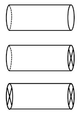
Figure 6.1: Two dimensional topologies where indices are defined. The first one denotes for a cylinder with two boundaries at the ends, and the second one corresponds to the Möbius strip with one boundary and one crosscap. The last one is the Klein bottle, with two crosscap states at the ends.

Following the discussion of the previous subsection, here we assume that an extra factor $e^{d({\cal M})/2}$ is present not only on the world-volumes of D-branes but also on the world-volumes of Orientifold planes. Otherwise, amplitudes involving boundary states only and amplitude involving a boundary state and a crosscap cannot be summed up; this would lead to net world-volume anomaly and make the spacetime theory inconsistent. Because we assume ${\cal X}$ itself to be Spin, $d({\cal M})/2$ is always expressed as a sum over $-c_{1}/2$ of the normal bundles of the world-volumes. As we have not demonstrated the GLSM origin of this factor for Orientifolds, the readers may wish to regard the following with the assumption of $d=0$, that is, only for Spin ${\cal M}$’s.

Cylinder

Index on the cylinder and relation to the disk partition function were studied in [7] and [9].

We start with Eq. (6.3) and use the relation (6.12) to calculate the open string index stretched between two branes with $({\cal E}_{1},{\cal M}_{1})$ and $({\cal E}_{2},{\cal M}_{2})$ as

$$I({\cal B}_{{\cal E}_{1}},{\cal B}_{{\cal E}_{2}})$$

$$\sim \int_{{\cal M}_{1}\cap{\cal M}_{2}}e^{-B-iJ}\wedge ch({\cal E}_{1})\wedge\frac{\hat{\Gamma}_{c}({\cal T}_{1})}{\hat{\Gamma}_{c}(-{\cal N}_{1})}\wedge e^{d({\cal M}_{1})/2}$$

$$\phantom{qqqqqqq}\wedge e^{B+iJ}\wedge ch(-{\cal E}_{2})\wedge\frac{\hat{\Gamma}_{c}(-{\cal T}_{2})}{\hat{\Gamma}_{c}({\cal N}_{2})}\wedge e^{-d({\cal M}_{2})/2}\wedge e({\cal N}_{12})$$

$$= \int_{{\cal M}_{1}\cap{\cal M}_{2}}ch({\cal E}_{1})\wedge ch(-{\cal E}_{2})\wedge\frac{{\cal A}({\cal T}({\cal M}_{1}\cap{\cal M}_{2}))}{{\cal A}({\cal N}({\cal M}_{1}\cap{\cal M}_{2}))}\wedge e^{\left(d({\cal M}_{1})-d({\cal M}_{2})\right)/2}\wedge e({\cal N}_{12})\ ,$$

where ${\cal T}_{i}$ and ${\cal N}_{i}$ denote for tangent and normal bundles of ${\cal M}_{i}$ and ${\cal N}_{12}\equiv{\cal N}_{1}\cap{\cal N}_{2}$. From the first to the second line, we used

$$\frac{\hat{\Gamma}_{c}({\cal T}_{1})\wedge\hat{\Gamma}_{c}(-{\cal T}_{2})}{\hat{\Gamma}_{c}(-{\cal N}_{1})\wedge\hat{\Gamma}_{c}({\cal N}_{2})}=\frac{\hat{\Gamma}_{c}({\cal T}_{1}\cap{\cal T}_{2})\hat{\Gamma}_{c}(-{\cal T}_{1}\cap{\cal T}_{2})}{\hat{\Gamma}_{c}(-{\cal N}_{1}\cap{\cal N}_{2})\hat{\Gamma}_{c}({\cal N}_{1}\cap{\cal N}_{2})}=\frac{{\cal A}({\cal T}_{1}\cap{\cal T}_{2})}{{\cal A}({\cal N}_{1}\cap{\cal N}_{2})}\ ,$$ (6.16)

since

$${\cal T}_{1}\backslash({\cal T}_{1}\cap{\cal T}_{2})={\cal N}_{2}\backslash({\cal N}_{1}\cap{\cal N}_{2})\ .$$ (6.17)

Note that, for the first equality, complex conjugation of the normal bundle in the denominator of Eq. (6.3) is essential.

The factor $e^{\left(d({\cal M}_{1})-d({\cal M}_{2})\right)/2}$ in (6.3) can be understood from the fact that the I-brane fermions on ${\cal M}_{1}\cap{\cal M}_{2}$ are naturally sections of ${\cal S}({\cal T}_{1}\cap{\cal T}_{2}\oplus{\cal N}_{1}\cap{\cal N}_{2})$. When the latter fails to be Spin, the 2nd Stiefel-Whitney class that measures this failure is

$$w_{2}({\cal T}_{1}\cap{\cal T}_{2}\oplus{\cal N}_{1}\cap{\cal N}_{2})=w_{2}({\cal T}_{1})-w_{2}({\cal T}_{2})\ ,$$

where the equality follows from the assumption that the ambient ${\cal X}$ is Spin. Since $w_{2}=c_{1}$ mod $Z_{2}$, the relevant correcting factor for the Spin^c case is $e^{(c_{1}({\cal T}_{1})-c_{1}({\cal T}_{2}))/2}$. Note that this factor reduces to 1 when ${\cal M}_{1}$ and ${\cal M}_{2}$ are coincident, which is expected since ${\cal T}\oplus{\cal N}={\cal T}{\cal X}$ is Spin. Next, we show how this extends to amplitudes involving Orientifold planes.

Möbius strip

Similarly, the index on the Möbius strip can be obtained via the relation (6.13). If we let ${\cal M}_{1}$ and ${\cal M}_{2}$ are locus where D-branes and Orientifolds exist, we have

$$I({\cal B}_{\cal E},{\cal C}) \sim 2^{p-4}\int_{{\cal M}_{1}\cap{\cal M}_{2}}ch_{2k}({\cal F})\wedge\frac{\hat{\Gamma}({{\cal T}_{1}})}{\hat{\Gamma}(-{{\cal N}_{1}})}\wedge\frac{{\cal A}({{\cal T}_{2}}/2)\hat{\Gamma}(-{{\cal N}_{2}})}{{\cal A}({{\cal N}_{2}}/2)\hat{\Gamma}({{\cal T}_{2}})}\wedge e^{\left(d({\cal M}_{1})-d({\cal M}_{2})\right)/2}\wedge e({\cal N}_{12})$$ (6.18)

$$= 2^{p-4}\int_{{\cal M}_{1}\cap{\cal M}_{2}}ch_{2k}({\cal F})\wedge\sqrt{\frac{{\cal A}({\cal T}_{1}){\cal L}({\cal T}_{2}/4)}{{\cal A}({\cal N}_{1}){\cal L}({\cal N}_{2}/4)}}\wedge e^{\left(d({\cal M}_{1})-d({\cal M}_{2})\right)/2}\wedge e({\cal N}_{12})\ ,$$

which exactly reproduce the index formula of the Möbius strip calculated at the level of non-linear sigma model [29, 14]. Here, $p+1$ is the dimension of the Orientifold plane.

When D$p$-branes are on the top of an O$p$-plane, in particular, we can read off $p+3$-form from $I({\cal B}_{E},{\cal C})+I({\cal C},{\cal B}_{E})$, which gives anomaly inflow on the $p+1$ dimensional world-volume as

$$\pm~{}2^{p-4}\cdot[ch_{2k}({\cal F})+ch_{\overline{2k}}({\cal F})]\wedge\frac{\hat{\Gamma}({\cal T})}{\hat{\Gamma}(-{\cal N})}\wedge\frac{{\cal A}({\cal T}/2)\hat{\Gamma}(-{\cal N})}{{\cal A}({\cal N}/2)\hat{\Gamma}({\cal T})}\wedge e({\cal N})~{}\Bigg{|}_{p+3}$$ (6.19)

$$= \pm~{}2^{p-4}\cdot\left[ch_{2k}({\cal F})+ch_{\overline{2k}}({\cal F})\right]\wedge\frac{{\cal A}({\cal T}/2)}{{\cal A}({\cal N}/2)}\wedge e({\cal N})~{}\Bigg{|}_{p+3}$$

$$= \pm~{}ch_{2k}(2{\cal F})\wedge\frac{{\cal A}({\cal T})}{{\cal A}({\cal N})}\wedge e({\cal N})~{}\Bigg{|}_{p+3}\ .$$

Note that, since $U(k)$ gauge group is enhanced to $SO(2k)$ or $Sp(k)$ group, we used the relation $ch_{2k}({\cal F})=ch_{\overline{2k}}({\cal F})$. Adding two contributions from the cylinder and the Möbius indices, we recover the open string Witten index, i.e., anomaly inflow for the $SO(2N)$ or $Sp(N)$ gauge group according to the sign of (6.19),

$$I_{SO(2k),Sp(k)} = [ch_{2k\otimes 2k}({\cal F})\pm ch_{2k}(2{\cal F})]\wedge\frac{{\cal A}({\cal T})}{{\cal A}({\cal N})}\wedge e({\cal N})\Bigg{|}_{p+3}$$ (6.20)

$$= 2\cdot ch_{\frac{1}{2}2k(2k\pm 1)}\wedge\frac{{\cal A}({\cal T})}{{\cal A}({\cal N})}\wedge e({\cal N})\Bigg{|}_{p+3}\ .$$

Klein bottle

Finally, if there are two crosscap states as in the last diagram of the figure, we have topology of the Klein bottle whose index is given by the relation (6.14). Substituting our formula for the crosscap overlap into this identity, we have

$$I({\cal C},{\cal C}) \sim 2^{p_{1}+p_{2}-8}\int_{{\cal M}_{1}\cap{\cal M}_{2}}\frac{{\cal A}({\cal T}_{1}/2)\hat{\Gamma}({\cal N}_{1})}{{\cal A}({\cal N}_{1}/2)\hat{\Gamma}(-{\cal T}_{1})}\wedge\frac{{\cal A}({\cal T}_{2}/2)\hat{\Gamma}(-{\cal N}_{2})}{{\cal A}({\cal N}_{2}/2)\hat{\Gamma}({\cal T}_{2})}\wedge e^{\left(d({\cal M}_{1})-d({\cal N}_{2})\right)/2}\wedge e({\cal N}_{12})$$ (6.21)

$$= 2^{p_{1}+p_{2}-8}\int_{{\cal M}_{1}\cap{\cal M}_{2}}\left(\frac{{\cal A}({\cal T}_{1}\cap{\cal T}_{2}/2)}{{\cal A}({\cal N}_{1}\cap{\cal N}_{2}/2)}\right)^{2}\wedge\frac{{\cal A}({\cal N}_{1}\cap{\cal N}_{2})}{{\cal A}({\cal T}_{1}\cap{\cal T}_{2})}\wedge e^{\left(d({\cal M}_{1})-d({\cal M}_{2})\right)/2}\wedge e({\cal N}_{12})$$

$$= 2^{p_{1}+p_{2}-8}\int_{{\cal M}_{1}\cap{\cal M}_{2}}\frac{{\cal L}({\cal T}_{1}\cap{\cal T}_{2}/4)}{{\cal L}({\cal N}_{1}\cap{\cal N}_{2}/4)}\wedge e^{\left(d({\cal M}_{1})-d({\cal M}_{2})\right)/2}\wedge e({\cal N}_{12})\ .$$

This again gives the well-known formula for the Klein bottle index calculated in non-linear sigma model. Since the B-type parity action corresponds to the Hodge star operation of the target space, it reproduces the Hirzebruch signature theorem [14]. Obviously, this index is independent of the open string degrees of freedom, or the types of planes [32]. For type-I string theory, this inflow precisely cancels the one-loop anomaly of supergravity multiplet.

6.4 RR-Charges and Quantum Volumes

This brings us, finally, to a natural question of what part of the central charge should be attributed to the RR-charges. Recall that the conventional RR-charges, or the Chern-Simons coupling to RR-tensors, was deduced indirectly via anomaly inflow. For instance, for the simplest case of the spacetime-filling D-brane, the relevant anomaly polynomial is ${\cal A}({\cal T})$, the $\hat{A}$ class, which is then reconstructed via inflow as

$$\Omega({\cal T})\wedge\Omega(-{\cal T})={\cal A}({\cal T})\ ,$$ (6.22)

where $\Omega$ is the characteristic class that appears in the Chern-Simons coupling. With an implicit assumption that $\log\Omega$ is “even,” i.e., includes $4k$-forms only, this leads to $\Omega={\cal A}^{1/2}$ [27, 28, 23]. Some of early literatures were casual about distinction between $\Omega({\cal T})$ and $\Omega(-{\cal T})$, although more careful computations show the conjugation has to occur for one of the two factors [28, 32]. Thus, in hindsight, the anomaly cancelation argument fixes only “even” part of $\log\Omega$.

As was noted previously, $\Omega=\hat{\Gamma}_{c}$ is one multiplicative class that is consistent with the anomaly inflow ${\cal A}$ in the above sense. This happens precisely because “even” part of $\log\hat{\Gamma}_{c}$ coincides exactly with $\log{\cal A}^{1/2}$. Our discussion in the previous section demonstrated that replacements like

$${\cal A}^{1/2}({\cal T})\rightarrow\hat{\Gamma}_{c}({\cal T}),\qquad{\cal L}^{1/2}({\cal T}/4)\rightarrow{\cal A}({\cal T}/2)/\hat{\Gamma}_{c}(-{\cal T})\ ,$$ (6.23)

for D-branes and Orientifold planes, respectively, would be still consistent with anomaly inflow. However, since the central charge is made from RR-charges and quantum volumes of various cycles, it is hardly clear whether such a change in the central charge should be attributed to the RR-charge or not.

More generally, for a D-brane wrapping a cycle ${\cal M}$ in Calabi-Yau ${\cal X}$, the gravitational curvature contribution to the central charge is

$$\frac{\hat{\Gamma}_{c}({\cal T})}{\hat{\Gamma}_{c}(-{\cal N})}=\sqrt{\frac{{\cal A}({\cal T})}{{\cal A}({\cal N})}}\wedge\exp\left(\,i\,\sum_{k\geq 1}\frac{(-1)^{k}(2k)!\zeta(2k+1)}{(2\pi)^{2k}}ch_{2k+1}({\cal X})\right)\ ,$$ (6.24)

so the deviation depends only on ${\cal X}$. As shown in the present work, something quite similar happens for the Orientifold planes,

$$\frac{{\cal A}({\cal T}/2)}{\hat{\Gamma}_{c}(-{\cal T})}\frac{\hat{\Gamma}_{c}({\cal N})}{{\cal A}({\cal N}/2)}=\sqrt{\frac{{\cal L}({\cal T}/4)}{{\cal L}({\cal N}/4)}}\wedge\exp\left(\,i\,\sum_{k\geq 1}\frac{(-1)^{k}(2k)!\zeta(2k+1)}{(2\pi)^{2k}}ch_{2k+1}({\cal X})\right)\ ,$$ (6.25)

where the deviation is identical to its D-brane counterpart. So the difference between the new central charges and the conventional ones can be expressed by a universal factor, determined by ${\cal X}$ only, is independent of the choice of the cycle ${\cal M}$, and its logarithm is purely imaginary.

These properties all suggest that this factor should be interpreted as a $\alpha^{\prime}$ modification of volumes, in the sense,

$$\exp(-iJ)\quad\rightarrow\quad\exp\left(-iJ+\,i\,\sum_{k\geq 1}\frac{(-1)^{k}(2k)!\zeta(2k+1)}{(2\pi)^{2k}}ch_{2k+1}({\cal X})\right)\ ,$$ (6.26)

rather than as a shift of RR-charges, or the Chern-Simons couplings, themselves. In fact, this is precisely the same shift of $J$ that appears in $S^{2}$ partition function, or its large volume expression,

$$Z_{S^{2}} \sim \int_{\cal X}e^{-2iJ}\wedge\frac{\hat{\Gamma}_{c}({\cal T}{\cal X})}{\hat{\Gamma}_{c}(-{\cal T}{\cal X})}$$ (6.27)

$$= \int_{\cal X}\;\exp\left(-2iJ+\,2i\,\sum_{k\geq 1}\frac{(-1)^{k}(2k)!\zeta(2k+1)}{(2\pi)^{2k}}ch_{2k+1}({\cal X})\right)\ .$$ (6.28)

Here, the “even” part of the two Gamma classes cancel out completely, suggesting that they, but not “odd” parts, carry RR-charge information. For Calabi-Yau 3-fold, the piece $\int_{\cal X}ch_{3}({\cal X})$ is proportional to the Euler number and represents exactly the quantum shift of the volume that has been seen in the mirror map [2, 13]. This viewpoint also conforms with the fact that there is no modification for Calabi-Yau 2-fold (times remaining flat directions), for which the ten-dimensional spacetime theory has as many as 16 supercharges.

The ambiguity in determining RR-charge from the anomaly inflow remains, as the D-brane and the I-brane inflow mechanisms always conjugate one of the two factors as in (6.22). However, once we accept (6.26) as the quantum version of the exponentiated Kähler class, this ambiguity is lifted, and we come back to the same old Chern-Simons coupling to spacetime RR-tensors for D-branes and Orientifold planes [23, 27, 28, 29, 30, 31, 32].

Acknowledgement

We benefited from discussions and communications with Dongmin Gang, Jaume Gomis, Jeff Harvey, Kentaro Hori, Emil Martinec, Takuya Okuda, and Savdeep Sethi. S.L. thanks the Perimeter Institute for hospitality where part of this work has been done. This work is supported in part (H.K.) by NRF(National Research Foundation of Korea) Grant funded by the Korean Government (NRF-2011-Global Ph.D. Fellowship Program), and also (S.L.) by the Ernest Rutherford fellowship of the Science and Technology Facilities Council ST/J003549/1.

Appendix

Appendix A Spherical Harmonics

We summarize basic facts about the (monopole) spherical harmonics. In order to discuss the projection condition under the parity, it is convenient to choose a gauge where the monopole background vector field takes the following form

$$A=-\frac{B}{2}\cos\theta d\varphi\ ,$$ (A.1)

valid in the region $0<\theta<\pi$. In addition, we also need to choose a gauge for the spin connection, as it affects the harmonics for spinors and vectors. Our choice,

$$w^{\hat{\theta}}_{\;\;\hat{\phi}}=-\cos\theta d\varphi\ ,$$ (A.2)

is such that spinor spherical harmonics are antiperiodic along $\phi\rightarrow\phi+2\pi$.

The scalar monopole harmonics $Y_{\mathbf{q},jm}$ with $\mathbf{q}=\frac{B}{2}Q$ satisfy

$$-D_{m}^{2}Y_{\mathbf{q},jm}=j(j+1)-\mathbf{q}^{2}\ ,\qquad j=l+|\mathbf{q}|\ (l=0,1,2,..)\ ,$$ (A.3)

where the covariant derivative denotes

$$D=d-iQA\ .$$ (A.4)

For later convenience, we present an explicit expression of the scalar monopole harmonics below,

$$Y_{\mathbf{q},jm}(\theta,\varphi)=M_{\mathbf{q},jm}(1-x)^{\alpha/2}(1+x)^{\beta/2}P_{n}^{\alpha\beta}(x)e^{im\varphi}\ ,$$ (A.5)

with

$$x=\cos\theta\ ,\ \alpha=-\mathbf{q}-m\ ,\ \beta=\mathbf{q}-m\ ,\ n=j+m\ ,$$ (A.6)

and

$$M_{\mathbf{q},jm}=2^{m}\sqrt{\frac{2j+1}{4\pi}\frac{(j-m)!(j+m)!}{(j-\mathbf{q})!(j+\mathbf{q})!}}\ .$$ (A.7)

Here the Jacobi polynomial $P_{n}^{\alpha\beta}(x)$ is defined by

$$P_{n}^{\alpha\beta}(x)=\frac{(-1)^{n}}{2^{n}n!}(1-x)^{-\alpha}(1+x)^{-\beta}\frac{d^{n}}{dx^{n}}\Big{[}(1-x)^{\alpha+n}(1+x)^{\beta+n}\Big{]}\ .$$ (A.8)

Using the fact that

$$P_{n}^{\alpha\beta}(-x)=(-1)^{n}P_{n}^{\beta\alpha}(x)\ ,$$ (A.9)

it is straightforward to show that, for $0<\theta<\pi$,

$$Y_{\mathbf{q},jm}(\pi-\theta,\pi+\varphi)= (-1)^{n}e^{i\pi m}\,Y_{-\mathbf{q},jm}(\theta,\varphi)$$

$$= (-1)^{l}e^{-i\pi|\mathbf{q}|}\,Y_{-\mathbf{q},jm}(\theta,\varphi)\ .$$ (A.10)

For instance,

$$Y_{\pm\frac{1}{2},jm}(\pi-\theta,\pi+\varphi)=(-i)(-1)^{l}Y_{\mp\frac{1}{2},jm}(\theta,\varphi)\ \text{for }j=l+\frac{1}{2}\ .$$ (A.11)

The complex conjugate of the monopole harmonics satisfy the following two relations,

$$Y_{\mathbf{q},jm}^{*}(\theta,\varphi)=(-1)^{\mathbf{q}+m}Y_{-\mathbf{q},j(-m)}(\theta,\varphi)\ ,$$ (A.12)

and

$$\int_{S^{2}}\ Y_{\mathbf{q},jm}^{*}(\theta,\varphi)Y_{\mathbf{q^{\prime}},j^{\prime}m^{\prime}}(\theta,\varphi)=\delta_{qq^{\prime}}\delta_{jj^{\prime}}\delta_{mm^{\prime}}\ .$$ (A.13)

We now move on to the spinor monopole harmonics. It is useful to consider the eigenmodes $\Psi^{\pm}_{\mathbf{q},jm}$ of a modified Dirac operator

$$-i\gamma^{3}\gamma^{m}D_{m}\Psi^{\pm}_{\mathbf{q},jm}=i\lambda_{\pm}\Psi^{\pm}_{\mathbf{q},jm}\ ,\qquad\lambda_{\pm}=\pm\sqrt{\left(j+\frac{1}{2}\right)^{2}-\mathbf{q}^{2}}\ ,$$ (A.14)

where

$$\Psi^{\pm}_{\mathbf{q},jm}=\begin{pmatrix}Y_{\mathbf{q}-\frac{1}{2},jm}\\ \pm Y_{\mathbf{q}+\frac{1}{2},jm}\end{pmatrix}\ .$$ (A.15)

Here the covariant derivative is

$$D=d-iQA+\frac{1}{4}\omega_{ab}\gamma^{ab}\ .$$ (A.16)

Using the property of the monopole harmonics (A.11), one can show

$$\Psi_{\mathbf{q}=0,jm}^{\pm}(\pi-\theta,\pi+\varphi)=\mp i(-1)^{l}\begin{pmatrix}\pm Y_{\frac{1}{2},jm}(\theta,\varphi)\\ Y_{-\frac{1}{2},jm}(\theta,\varphi)\end{pmatrix}\ ,$$ (A.17)

with $0<\theta<\pi$.

Finally let us discuss about the one-form spherical harmonics defined by

$$C^{1}_{jm}= +\frac{1}{\sqrt{j(j+1)}}dY_{lm}\ ,$$

$$C^{2}_{jm}= -\frac{1}{\sqrt{j(j+1)}}\ast dY_{jm}\ ,$$ (A.18)

where $j\geq 1$. Useful properties of the vector spherical harmonics can be summarized as follow,

$$\ast C^{2}_{jm}=C^{1}_{jm}\ ,\qquad\ast dC^{2}_{jm}=\sqrt{j(j+1)}Y_{lm}\ ,\qquad\ast dC^{1}_{jm}=0\ ,$$ (A.19)

which lead to

$$\ast d\ast dC^{2}_{jm}= -j(j+1)C^{2}_{jm}\ ,$$

$$\ast d\ast dC^{1}_{jm}= \ 0\ .$$ (A.20)

Under the parity action, they transform as

$$C^{1}_{jm}(\pi-\theta,\pi+\varphi)= \ (-1)^{j}C^{1}_{jm}(\theta,\varphi)\ ,$$

$$C^{2}_{jm}(\pi-\theta,\pi+\varphi)= \ (-1)^{j+1}C^{2}_{jm}(\theta,\varphi)\ .$$ (A.21)

Appendix B One-Loop Determinant on $\mathbb{RP}^{2}_{b}$

We will show that the partition function on the squashed real projective space $\mathbb{RP}^{2}_{b}$ is independent of the squashing parameter $b$. This section largely relies on the discussion in [3]. For details, please refer to Appendix A of the reference.

To compute the one-loop determinant around the SUSY saddle points, it is not necessary to know all the eigenmodes of boson and fermion kinetic operators. This is because, as we see in section 3, the huge cancelation between boson and fermion eigenmodes occurs. It is therefore sufficient to understand how the boson and fermion eigenmodes are paired by the supersymmetry.

B.1 Chiral multiplet

We start with a chiral multiplet of unit $U(1)$ gauge charge. To simplify the computation, we choose a ${\cal Q}$-exact regulator

$${\cal L}_{\text{reg}}=-\delta_{\epsilon}\delta_{\bar{\epsilon}}\Big{[}\bar{\psi}\gamma^{3}\psi-2\bar{\phi}\sigma_{2}\phi\Big{]}\ ,$$ (B.1)

different to the one used in the main context. The above choice leads to the kinetic operators around the saddle points (3.1), (3.2)

$$\Delta_{b}= -D_{m}^{2}+\sigma^{2}+\frac{q}{4}{\cal R}+\frac{q-1}{f}v^{m}D_{m}++\frac{q^{2}-2q}{4f^{2}}\ ,$$

$$\Delta_{f}= -i\gamma^{m}D_{m}-\sigma\gamma^{3}-i\frac{1}{2f}\gamma^{3}+i\frac{q-1}{2f}v_{m}\gamma^{m}+i\frac{q-1}{2f}w\ ,$$ (B.2)

where the covariant derivative involves the background gauge field $V$ given in (2.28),

$$D_{m}\phi= \left(\partial_{m}-iA_{m}+iqV_{m}\right)\phi\ ,$$

$$D_{m}\psi= \left(\partial_{m}-iA_{m}+\frac{1}{4}w_{ab}\gamma^{ab}+i(q-1)V_{m}\right)\psi\ ,$$ (B.3)

and

$$v^{m}=\bar{\epsilon}\gamma^{m}\epsilon\ ,\qquad w=\bar{\epsilon}\epsilon\ .$$ (B.4)

Here ${\cal R}$ denotes the scalar curvature of $\mathbb{RP}^{2}$. As in section 3, it is convenient to consider spinor eigenmodes for an operator $\gamma^{3}\Delta_{f}$ instead of $\Delta_{f}$.

One can show that there is a pair between a scalar eigenmode for $\Delta_{b}\doteq-M(M+2\sigma)$ and two spinor eigenmodes for $\gamma^{3}\Delta_{f}\doteq M,-(M+2\sigma)$, subject to either (3.8) or (3.22) projection conditions. The precise map which pairs the scalar and spinor eigenmodes is the following; Given a spinor eigenmode $\Psi$ for $\gamma^{3}\Delta_{f}\doteq M$, one can show that

$$\bar{\epsilon}\Psi$$ (B.5)

is a scalar eigenmode for $\Delta_{b}\doteq-M(M+2\sigma)$. On the other hand, one can define a pair of spinors

$$\Psi_{1}=\gamma^{3}\epsilon\Phi\ ,\qquad\Psi_{2}=i\gamma^{m}\epsilon D_{m}\Phi+\gamma^{3}\epsilon\left(\sigma\Phi+i\frac{q}{2f}\right)\Phi\ ,$$ (B.6)

where $\Phi$ is a scalar eigenmode for $\Delta_{b}\doteq-M(M+2\sigma)$. One can show that

$$M\Psi_{1}+\Psi_{2}\ ,\qquad-(M+2\sigma)\Psi_{1}+\Psi_{2}$$ (B.7)

are the eigenmodes for $\gamma^{3}\Delta_{f}\doteq M$ and $\gamma^{3}\Delta_{f}\doteq-(M+2\sigma)$ respectively.

Any modes in such a pair can not contribute to the one-loop determinant due to the cancelation. As a consequence, the nontrivial contributions arise from the eigenmodes where either the map (B.5) or the map (B.7) becomes ill-defined.

Unpaired spinor eigenmode

If a spinor eigenmode vanishes when contracted with $\bar{\epsilon}$, there is no scalar partner. Such an unpaired spinor eigenmode takes the following form

$$\Psi=e^{-iJ\varphi}h(\theta)\bar{\epsilon}\ ,$$ (B.8)

where

$$iJ=\left(Ml+\sigma l+i\frac{q-2}{2}\right)\ ,$$ (B.9)

and

$$\frac{1}{f}\partial_{\theta}h=\tan\theta\left(\frac{J}{l}-\frac{q-2}{2l}+i\frac{q-2}{2f}\right)h\ .$$ (B.10)

For the normalizability, one has to require $J$ to be non-negative. Note that the function $h(\theta)$ is even under the parity, i.e., $h(\theta)=h(\pi-\theta)$. One can show that $J$ should be further restricted to be even (odd) to satisfy the projection conditions in the even (odd) holonomy, i.e.,

$$Ml= i\left(2k+1+i\sigma l-\frac{q}{2}\right)\text{ for even holonomy}\ ,$$

$$Ml= i\left(2k+2+i\sigma l-\frac{q}{2}\right)\text{ for odd holonomy}\ ,$$ (B.11)

with $k\geq 0$.

Missing spinor eigenmode

Suppose that a scalar eigenmode $\Phi$ for $\Delta_{b}\doteq-M(M+2\sigma)$ fails to provide two independent spinor eigenmodes via the map (B.7). It happens when

$$\Psi_{2}=-M\Psi_{1}\ ,$$ (B.12)

which leads to a missing spinor eigenmode for $\gamma^{3}\Delta_{f}\doteq M$. One can verify that such a scalar eigenmode $\Phi$ missing a spinor eigenmode takes the following form

$$\Phi=e^{iJ\varphi}\chi(\theta)\ ,$$ (B.13)

where

$$iJ=-\left(Ml+\sigma l+i\frac{q}{2}\right)\ ,$$ (B.14)

with $J\geq 0$ for the normalizability, and

$$\frac{1}{f}\partial_{\theta}\chi=\tan\theta\left(\frac{J}{l}+\frac{q}{2l}-\frac{q}{2f}\right)\chi\ .$$ (B.15)

To satisfy the projection condition in the even (odd) holonomy, one can show that

$$Ml= -i\left(2k-i\sigma l+\frac{q}{2}\right)\text{ for even holonomy }\ ,$$

$$Ml= -i\left(2k+1-i\sigma l+\frac{q}{2}\right)\text{ for odd holonomy }\ ,$$ (B.16)

with $k\geq 0$.

One-loop determinant

Combining all the results (B.11) and (B.16), one can show

$$\frac{\det\Delta_{f}}{\det\Delta_{b}}\simeq \frac{\det\gamma^{3}\Delta_{f}}{\det\Delta_{b}}\simeq\left\{\begin{array}[]{cc}\prod_{k\geq 0}\frac{2k+1+i\sigma l-\frac{q}{2}}{2k-i\sigma l+\frac{q}{2}}&\text{for even holonomy}\\ \prod_{k\geq 0}\frac{2k+2+i\sigma l-\frac{q}{2}}{2k+1-i\sigma l+\frac{q}{2}}&\text{for odd holonomy}\end{array}\right.\ ,$$ (B.19)

where the symbol $\simeq$ represents the equality up to a sign independent of $\sigma$. From the comparison to the results in section 3, one can fix the sign factor by the unity. These results are in perfect agreement to those for $\mathbb{RP}^{2}$.

B.2 Vector multiplet

We now in turn compute the one-loop determinant from the vector multiplet. Denoting the various fluctuation fields as follows

$$A=A_{\text{flat}}+a\ ,\qquad\sigma_{1}=\zeta\ ,\qquad\sigma_{2}=\sigma+\eta\ ,$$ (B.20)

let us decompose all the adjoint fields $(a,\zeta,\eta)$ into Cartan-Weyl basis. From now on, we focus on the W-boson of charge $\alpha$, a root of $G$, and its super partners. The kinetic Lagrangian for the vector multiplet is chosen as a ${\cal Q}$-exact regulator.

As explained in [6] and [3] that the four bosonic modes contain two longitudinal modes with $a\sim D\eta$ that correspond to a gauge rotation and the volume of the gauge group $G$. Using the standard Fadeev-Popov method, one can argue that these longitudinal modes can not contribute to the one-loop determinant. Thus we need to find how two transverse modes with $\ast D\ast a=0$ can be paired with spinor eigenmodes.

The kinetic operators of our interest are

$$\Delta_{b}= \begin{pmatrix}-\ast d\ast d+(\alpha\cdot\sigma)^{2}&-\ast d\frac{1}{f}\\ +\frac{1}{f}\ast d&-\ast d\ast d+\frac{1}{f^{2}}+(\alpha\cdot\sigma)^{2}\end{pmatrix}\ ,$$

$$\Delta_{f}= i\gamma^{m}D_{m}+(\alpha\cdot\sigma)\gamma^{3}\ ,$$ (B.21)

with the gauge choice $\ast d\ast a=0$. The operator $\Delta_{b}$ acts on the fluctuation fields $(a,\zeta)$ subject to the projection conditions (3.34) for the even holonomy and the twisted projection conditions for the odd holonomy. Instead of $\Delta_{b}$, it is convenient to consider the following operator

$$\delta_{b}\equiv\begin{pmatrix}i\alpha\cdot\sigma&-\ast d\\ \ast d&\frac{1}{f}+i\alpha\cdot\sigma\end{pmatrix}\ .$$ (B.22)

One can show that the operator $\delta_{b}$ satisfies the relation $\delta_{b}^{2}=\Delta_{b}+2i(\alpha\cdot\sigma)\delta_{b}$, or equivalently,

$$\delta_{b}\doteq-iM\ ,+i(M+2\alpha\cdot\sigma)\ \leftrightarrow\ \Delta_{b}\doteq-M(M+2\alpha\cdot\sigma)\ .$$ (B.23)

Let $({\cal A},\Sigma)$ and $\Lambda$ be bosonic eigenmodes for $\delta_{b}\doteq-iM$ and fermionic eigenmodes for $\gamma^{3}\Delta_{f}\doteq-M$. They can be shown to be mapped to each other by

$${\cal A}=-i\left(M+\alpha\cdot\sigma\right)\bar{\epsilon}\gamma_{m}\Lambda e^{m}-d\left(\bar{\epsilon}\gamma^{3}\Lambda\right)\ ,\qquad\Sigma=(M+\alpha\cdot\sigma)\bar{\epsilon}\Lambda\ ,$$ (B.24)

and

$$\Lambda=\left(\gamma^{3}\gamma^{m}{\cal A}_{m}+i\Sigma\gamma^{3}\right)\epsilon\ .$$ (B.25)

Again, one can have nontrivial contribution to the one-loop determinant from either unpaired or missing spinor eigenmodes.

Unpaired spinor eigenmodes

An unpaired spinor eigenmode, annihilated by the map (B.24), takes the following form

$$\Lambda=e^{-iJ\varphi}h(\theta)\bar{\epsilon}\ ,$$ (B.26)

where

$$i\left(J+1\right)=Ml+\alpha\cdot\sigma l\ ,$$ (B.27)

with $J\geq 0$ due to the normalizability, and

$$\frac{1}{f}\partial_{\theta}h+\tan\theta\left(\frac{1}{f}-\frac{J+1}{l}\right)h=0\ .$$ (B.28)

Note that the function $h(\theta)$ is even under the parity, $h(\pi-\theta)=h(\theta)$. In order to satisfy the projection conditions in the even (odd) holonomy, the non-negative integer $J$ should be further constrained to be odd (even), i.e.,

$$Ml= i\left(2k+2+i\alpha\cdot\sigma\right)\text{ for even holonomy}\ ,$$

$$Ml= i\left(2k+1+i\alpha\cdot\sigma\right)\text{ for odd holonomy}\ ,$$ (B.29)

with $k\geq 0$.

Missing spinor eigenmodes

One can show from the map (B.25) that a bosonic eigenmode with missing spinor partner can take the following form

$${\cal A}=e^{i(J+1)\varphi}\chi(\theta)\left(e^{1}+i\cos\theta\epsilon^{2}\right)\ ,\qquad\Sigma=ie^{i(J+1)\varphi}\chi(\theta)\sin\theta\ ,$$ (B.30)

where $e^{m}$ denotes the vielbein of $\mathbb{RP}^{2}_{b}$, and

$$i(J+1)=-\left(Ml+\alpha\cdot\sigma l\right)\ ,$$ (B.31)

and

$$\frac{1}{f}\partial_{\theta}\chi+\tan\theta\left(\frac{1}{f}-\frac{J+1}{l}\right)\chi=0\ .$$ (B.32)

The normalizability requires $J$ to be non-negative. The projection conditions in even (odd) holonomy are satisfied if $J$ are even (odd), i.e.,

$$Ml= -i\left(2k+1-i\alpha\cdot\sigma\right)\text{ for even holonomy}\ ,$$

$$Ml= -i\left(2k+2-i\alpha\cdot\sigma\right)\text{ for odd holonomy}\ ,$$ (B.33)

with $k\geq 0$.

One-loop determinant

Collecting all the results (B.29) and (B.33), the one-loop determinant from the vector multiplet becomes

$$\frac{\det\Delta_{f}}{\sqrt{\det\Delta_{b}}}\simeq\frac{\det\gamma^{3}\Delta_{f}}{\det\delta_{b}}\simeq \left\{\begin{array}[]{cc}\prod_{\alpha\in\Delta}\prod_{k\geq 0}\frac{2k+2+i\alpha\cdot\sigma}{2k+1-i\alpha\cdot\sigma}&\text{for even holonomy}\\ \prod_{\alpha\in\Delta}\prod_{k\geq 0}\frac{2k+1+i\alpha\cdot\sigma}{2k+2-i\alpha\cdot\sigma}&\text{for odd holonomy}\end{array}\ .\right.$$ (B.36)

By comparing the results to those in section 3, one can fix the sign factor by the unity. Again, these results perfectly agree with those for $\mathbb{RP}^{2}$.

Appendix C Spin^c Structure and Tachyon Condensation

The central charge of the D-branes is recently revisited from the exact hemisphere partition function computation [7, 9], which shows that $\hat{\Gamma}_{c}$ class replaces the ${\cal A}^{1/2}$ class. In this note, we computed central charges of Orientifold planes and show how $L^{1/2}$ class in the traditional central charge formula must be similarly modified in terms of ${\cal A}$ class and $\hat{\Gamma}_{c}$ class. The original formulae for the RR-charges and the central charges were motivated by anomaly inflow, which can potentially miss some of $(4k+2)$-form pieces in the exponent.

An odd fact is that the partition function computations, with Dirichlet condition explicitly imposed, also seem to miss a factor $e^{-c_{1}({\cal N})/2}$ that is necessary when ${\cal M}$ is a proper submanifold of ${\cal X}$ and is not Spin but only Spin^c. Here, we will outline how this factor re-emerges, at least, from the viewpoint of tachyon condensation. After presenting results in Refs. [7, 9], we compute the central charge of a lower-dimensional D-brane wrapping a hypersurface in the Calabi-Yau space, with careful consideration given to charge assignment of the vacua. From this computation, the subtle factor $e^{-c_{1}({\cal N})/2}$ is rescued.

In order to preserve the supersymmetry chosen as in (2.18) on the northern hemisphere, one has to add the Chan-Paton factor

$$\text{Tr}_{\cal V}\Big{[}{\cal P}\exp\left(-i\int d\varphi\ {\cal A}_{\varphi}\right)\Big{]}$$ (C.1)

with

$${\cal A}_{\varphi}= \rho_{\ast}\left(A_{\varphi}+i\sigma_{2}\right)-\frac{r_{\ast}}{2r}-i\Big{\{}{\cal Q},\bar{\cal Q}\Big{\}}$$

$$+\frac{1}{\sqrt{2}}\left(\psi_{+}^{i}-\psi_{-}^{i}\right)\partial_{i}{\cal Q}+\frac{1}{\sqrt{2}}\left(\bar{\psi}_{+}^{i}-\bar{\psi}_{-}^{i}\right)\partial_{i}\bar{\cal Q}\ .$$ (C.2)

Here ${\cal V}$ denotes a $Z_{2}$ graded Chan-Paton vector space. The tachyon profile ${\cal Q}(\phi)$ is an operator acting on the vector space ${\cal V}$, anti-commuting with fermions, and obeys the following relation

$$Q^{2}={\cal W}\cdot{\bf 1}_{\cal V}\ ,$$ (C.3)

where ${\cal W}(\phi)$ denotes a given superpotential. The $G\times U(1)_{v}$ representation of the Chan-Paton vector space ${\cal V}$ is specified by $\rho_{\ast}$ and $r_{\ast}$,

$$\rho(g)Q(\phi)\rho(g)^{-1}= \ Q(g\phi)\ ,$$

$$\lambda\cdot\lambda^{r_{\ast}}Q(\phi)\lambda^{-r_{\ast}}= \ Q(\lambda^{q}\phi)\ ,$$ (C.4)

where $g\in G$. The exact hemisphere partition function can be expressed by

$$Z_{D^{2}}\propto\frac{1}{\left|W(G)\right|}\int_{\mathfrak{t}}d\sigma\ e^{-2\pi i\xi_{\text{ren}}\text{tr}\sigma-\theta\text{tr}\sigma}\times\text{Tr}_{\cal V}\Big{[}e^{2\pi\rho_{\ast}(\sigma)+i\pi r_{\ast}}\Big{]}\times Z_{\text{1-loop}}$$ (C.5)

with

$$Z_{\text{1-loop}}=\prod_{\alpha>0}\Big{[}\alpha\cdot\sigma\sinh{\alpha\cdot\sigma}\Big{]}\prod_{w_{a}\in\mathbf{R^{a}}}\Gamma\left(\frac{q_{a}}{2}-iw_{a}\cdot\sigma\right)\ ,$$ (C.6)

where $\mathfrak{t}$ is the Cartan subalgebra of the gauge group $G$, and $W(G)$ is the Weyl group.

In what follows, we consider the $U(1)$ GLSM describing the degree $N$ hypersurface of $\mathbb{CP}^{N-1}$ studied in section 5 for simplicity.

$${\cal W}=PG_{N}(X^{i})\ ,$$ (C.7)

where $G_{N}(X^{i})$ denotes a homogeneous polynomial of degree $N$. This model describes the non-linear sigma model whose target space is a CY hypersurface $X$ in $\mathbb{CP}^{N-1}$.

Taking into account for the Knörrer map to relate the GLSM brane $\mathfrak{B}_{UV}$ to the NLSM brane $\mathfrak{B}_{IR}$ [24], one can show that

$$ch\big{[}\mathfrak{B}_{IR}\big{]}=\frac{1}{1-e^{-2\pi iN(q/2-i\sigma)}}\times\text{Tr}_{{\cal V}}\Big{[}e^{2\pi\rho_{\ast}(\sigma)+i\pi r_{\ast}}\Big{]}\ ,$$ (C.8)

where ${\cal V}$ denotes the Chan-Paton vector space of $\mathfrak{B}_{UV}$. Note that the Knörrer map also leads to the shift of the theta angle

$$\theta_{UV}=\theta_{IR}-\pi N\ .$$ (C.9)

The central charge of the NLSM brane $\mathfrak{B}_{IR}$ then takes the following form

$$Z\left(\mathfrak{B}_{IR}\right)=2i\pi\beta\int_{q/2-i\infty}^{q/2+i\infty}\frac{d\epsilon}{2\pi i}\ e^{2\pi\xi\epsilon-i\theta_{IR}\epsilon}\times\frac{N}{\epsilon^{N-1}}\times\frac{\Gamma(1+\epsilon)^{N}}{\Gamma(1+N\epsilon)}\times ch\big{[}\mathfrak{B}_{IR}\big{]}$$ (C.10)

with $\beta=(r\Lambda)^{c/6}/(2\pi)^{(N-2)/2}$. Focusing on the perturbative part of the central charge, one can finally obtain the large-volume expression [7, 9]

$$Z_{\text{pert}}\left(\mathfrak{B}_{IR}\right)= \left(2\pi i\right)^{N-2}\beta\int_{X}\ e^{-i\xi H-\frac{\theta_{IR}}{2\pi}H}\times\frac{\Gamma(1+\frac{H}{2\pi i})^{N}}{\Gamma(1+\frac{NH}{2\pi i})}\times ch\big{[}\mathfrak{B}_{IR}\big{]}$$

$$= \left(2\pi i\right)^{N-2}\beta\int_{X}\ e^{-iJ-B}\wedge\hat{\Gamma}_{c}(X)\wedge ch\big{[}\mathfrak{B}_{IR}\big{]}\ ,$$ (C.11)

where $H$ is the hyperplane class of $\mathbb{CP}^{N-1}$.

To be more concrete let us consider a tachyon profile ${\cal Q}$

$${\cal Q}=X^{a}\eta_{a}+P\tilde{\eta}+G_{N}\bar{\tilde{\eta}}\ ,$$ (C.12)

where the fermionic oscillators satisfy the following anti-commutation relations

$$\{\tilde{\eta},\bar{\tilde{\eta}}\}=1\ ,\qquad\{\eta_{a},\bar{\eta}_{b}\}=\delta_{ab}$$ (C.13)

with $a=1,2,..,n$. Since the boundary potential becomes

$$\Big{\{}{\cal Q},\bar{\cal Q}\Big{\}}=\sum_{a=1}^{n}|X^{a}|^{2}+|P|^{2}+|G_{N}(X^{i})|^{2}\ ,$$ (C.14)

the above tachyon profile describes a lower-dimensional brane wrapping a submanifold at $X^{a}=0$ in the Calabi-Yau space $X$ in the geometric phase. One can easily show that the Chern character of the brane $\mathfrak{B}_{IR}$ is

$$ch\big{[}\mathfrak{B}_{IR}\big{]}=e^{-\pi in\epsilon}\Big{(}2i\sin(\pi\epsilon)\Big{)}^{n}\ ,$$ (C.15)

where $\epsilon=q/2-i\sigma$. Then, the central charge of the brane in the large volume limit (C.11) can be written as

$$Z_{\text{pert}}\left(\mathfrak{B}_{IR}\right)= \left(2i\pi\right)^{N-1}\beta\int_{X}e^{-i\xi H-\frac{\theta_{IR}}{2\pi}H}\times\frac{\Gamma(1+\frac{H}{2\pi i})^{N-n}}{\Gamma(1-\frac{H}{2\pi i})^{n}\Gamma(1+\frac{NH}{2\pi i})}\times H^{n}\times e^{-\frac{nH}{2}}$$

$$= \left(2i\pi\right)^{N-1}\beta\int_{X}e^{-iJ-B}\wedge\frac{\hat{\Gamma}_{c}({\cal T})}{\hat{\Gamma}_{c}(-{\cal N})}\wedge e({\cal N})\wedge e^{-\frac{1}{2}c_{1}({\cal N})}\ .$$ (C.16)

Note that one can see the very subtle factor $e^{-c_{1}({\cal N})/2}$ emerges from the partition function computation again. As a byproduct, we also confirmed that the overall normalization factor $(2\pi i)^{N-1}\beta=(2\pi)^{N/2}i^{N-1}(r\Lambda)^{c/6}$ are the same for any dimensional D-branes, which is consistent with the tadpole comparison of the section 6 above.

What remains unclear to us is how this factor should be recovered when the Dirichlet boundary condition is imposed from the outset. For D-branes here, the result (C.16) obtained from the tachyon condensation exactly agrees with the central charge for a D-brane supporting an extra “line bundle” ${\cal O}(-n/2)$, which can be described by imposing the Dirichlet boundary condition on $X^{a}$ and adding Wilson loop of charge $\rho_{\ast}=-n/2$. The line bundle ${\cal O}(-n/2)$ accounts for the factor $e^{-\frac{1}{2}c_{1}({\cal N})}$ canceling the Freed-Witten global anomaly. As there is analog of neither tachyon condensation representation nor Wilson loop for Orientifold planes, however, a better understanding of this issue is needed for addressing central charges of all RR-charged objects.

References

• [1] E. Witten, “Phases of N=2 theories in two-dimensions,” Nucl. Phys. B 403 (1993) 159 [hep-th/9301042].
• [2] H. Jockers, V. Kumar, J. M. Lapan, D. R. Morrison and M. Romo, “Two-Sphere Partition Functions and Gromov-Witten Invariants,” arXiv:1208.6244 [hep-th].
• [3] J. Gomis and S. Lee, “Exact Kahler Potential from Gauge Theory and Mirror Symmetry,” JHEP 1304 (2013) 019 [arXiv:1210.6022 [hep-th]].
• [4] S. Cecotti and C. Vafa, “Topological antitopological fusion,” Nucl. Phys. B 367 (1991) 359.
• [5] N. Doroud, J. Gomis, B. Le Floch and S. Lee, “Exact Results in D=2 Supersymmetric Gauge Theories,” JHEP 1305 (2013) 093 [arXiv:1206.2606 [hep-th]].
• [6] F. Benini and S. Cremonesi, “Partition functions of N=(2,2) gauge theories on $S^{2}$ and vortices,” arXiv:1206.2356 [hep-th].
• [7] K. Hori and M. Romo, “Exact Results In Two-Dimensional (2,2) Supersymmetric Gauge Theories With Boundary,” arXiv:1308.2438 [hep-th].
• [8] S. Sugishita and S. Terashima, “Exact Results in Supersymmetric Field Theories on Manifolds with Boundaries,” arXiv:1308.1973 [hep-th].
• [9] D. Honda and T. Okuda, “Exact results for boundaries and domain walls in 2d supersymmetric theories,” arXiv:1308.2217 [hep-th].
• [10] A. Libgober, “Chern classes and the periods of mirrors,” Math.Res.Lett.,6,141 [math.AG/9803119]
• [11] H. Iritani. ”Real and integral structures in quantum cohomology I : toric orbifolds”, [math.AG/0712.2204]
• [12] L. Katzarkov, M. Kontsevich and T. Pantev, “Hodge theoretic aspects of mirror symmetry,” [math.AG/0806.0107]
• [13] J. Halverson, H. Jockers, J. M. Lapan and D. R. Morrison, “Perturbative Corrections to Kahler Moduli Spaces,” arXiv:1308.2157 [hep-th].
• [14] I. Brunner and K. Hori, “Orientifolds and mirror symmetry,” JHEP 0411 (2004) 005 [hep-th/0303135].
• [15] K. Hori and C. Vafa, “Mirror symmetry,” [hep-th/0002222].
• [16] N. Doroud and J. Gomis, “Gauge Theory Dynamics and Kahler Potential for Calabi-Yau Complex Moduli,” arXiv:1309.2305 [hep-th].
• [17] E. Witten, “Baryons and branes in anti-de Sitter space,” JHEP 9807 (1998) 006 [hep-th/9805112].
• [18] D. Gao and K. Hori, “On The Structure Of The Chan-Paton Factors For D-Branes In Type II Orientifolds,” arXiv:1004.3972 [hep-th].
• [19] J. Polchinski and Y. Cai, “Consistency of Open Superstring Theories,” Nucl. Phys. B 296 (1988) 91.
• [20] I. Brunner, K. Hori, K. Hosomichi and J. Walcher, “Orientifolds of Gepner models,” JHEP 0702 (2007) 001 [hep-th/0401137].
• [21] D. S. Freed and E. Witten, “Anomalies in string theory with D-branes,” Asian J. Math 3 (1999) 819 [hep-th/9907189].
• [22] S. H. Katz and E. Sharpe, “D-branes, open string vertex operators, and Ext groups,” Adv. Theor. Math. Phys.  6 (2003) 979 [hep-th/0208104].
• [23] R. Minasian and G. W. Moore, “K theory and Ramond-Ramond charge,” JHEP 9711 (1997) 002 [hep-th/9710230].
• [24] M. Herbst, K. Hori and D. Page, “Phases Of N=2 Theories In 1+1 Dimensions With Boundary,” arXiv:0803.2045 [hep-th].
• [25] J. Distler, D. S. Freed and G. W. Moore, “Orientifold Precis,” In *Sati, Hisham (ed.) et al.: Mathematical Foundations of Quantum Field theory and Perturbative String Theory* 159-171 [arXiv:0906.0795 [hep-th]].
• [26] J. Distler, D. S. Freed and G. W. Moore, “Spin structures and superstrings,” arXiv:1007.4581 [hep-th].
• [27] M. B. Green, J. A. Harvey, G. Moore, “I-Brane inflow and anomalous couplings on D-branes”, Class. Quant. Grav.  14 (1997) 47 [hep-th/9605033].
• [28] Y.-K.E. Cheung and Z. Yin, “Anomalies, branes, and currents”, Nucl. Phys. B 517 (1998) 69 [hep-th/9710206].
• [29] J. F. Morales, C. A. Scrucca and M. Serone, “Anomalous couplings for D-branes and O-planes,” Nucl. Phys. B 552 (1999) 291 [hep-th/9812071].
• [30] K. Dasgupta, D. P. Jatkar and S. Mukhi, “Gravitational couplings and Z(2) orientifolds,” Nucl. Phys. B 523 (1998) 465 [hep-th/9707224].
• [31] K. Dasgupta and S. Mukhi, “Anomaly inflow on orientifold planes,” JHEP 9803 (1998) 004 [hep-th/9709219].
• [32] H. Kim and P. Yi, “D-brane anomaly inflow revisited,” JHEP 1202 (2012) 012 [arXiv:1201.0762 [hep-th]].
• [33] B. Craps and F. Roose, “Anomalous D-brane and orientifold couplings from the boundary state,” Phys. Lett. B 445 (1998) 150 [hep-th/9808074].
• [34] B. Stefanski, Jr., “Gravitational couplings of D-branes and O-planes,” Nucl. Phys. B 548 (1999) 275 [hep-th/9812088].
• [35] B. Craps and F. Roose, “(Non)anomalous D-brane and O-plane couplings: The Normal bundle,” Phys. Lett. B 450 (1999) 358 [hep-th/9812149].
• [36] E. J. Weinberg, “Monopole vector spherical harmonics,” Phys. Rev. D 49 (1994) 1086 [hep-th/9308054].