Multivariate transient price impact and matrix-valued positive definite functions

Abstract

We consider a model for linear transient price impact for multiple assets that takes cross-asset impact into account. Our main goal is to single out properties that need to be imposed on the decay kernel so that the model admits well-behaved optimal trade execution strategies. We first show that the existence of such strategies is guaranteed by assuming that the decay kernel corresponds to a matrix-valued positive definite function. An example illustrates, however, that positive definiteness alone does not guarantee that optimal strategies are well-behaved. Building on previous results from the one-dimensional case, we investigate a class of nonincreasing, nonnegative, and convex decay kernels with values in the symmetric $K\times K$ matrices. We show that these decay kernels are always positive definite and characterize when they are even strictly positive definite, a result that may be of independent interest. Optimal strategies for kernels from this class are particularly well-behaved if one requires that the decay kernel is also commuting. We show how such decay kernels can be constructed by means of matrix functions and provide a number of examples. In particular, we completely solve the case of matrix exponential decay.

Keywords: Multivariate price impact, matrix-valued positive definite function, optimal trade execution, optimal portfolio liquidation, matrix function

1 Introduction

Price impact refers to the feedback effect of trades on the quoted price of an asset and it is responsible for the creation of execution costs. It is an empirically established fact that price impact is predominantly transient; see, e.g., Moro et al. (2009). When trading speed is sufficiently slow, the effects of transience can be reduced to considering only a temporary and a permanent price impact component (Bertsimas and Lo, 1998; Almgren and Chriss, 2001). For higher trading speeds, however, one needs a model that explicitly describes the decay of price impact between trades. First models of this type were proposed by Bouchaud et al. (2004) and Obizhaeva and Wang (2013). These models were later extended into various directions by Alfonsi et al. (2008, 2010), Gatheral (2010), Alfonsi et al. (2012), Gatheral et al. (2012), Predoiu et al. (2011), Fruth et al. (2014), and Løkka (2012), to mention only a few. A more comprehensive list of references can be found in Gatheral and Schied (2013). We also refer to Guo (2013) for an introduction to the microscopic order book picture that is behind the mesoscopic models mentioned above.

All above-mentioned models for transient price impact deal only with one single risky asset. While multi-asset models for temporary and permanent price impact (Schöneborn, 2011) or for generic price impact functionals (Schied et al., 2010; Kratz and Schöneborn, 2013) were considered earlier, we are not aware of any previous approaches to analyzing the specific effects of transient cross-asset price impact. Our goal in this paper is to propose and analyze a simple model for transient price impact between $K$ different risky assets. Following the one-dimensional ansatz of Gatheral (2010), the time-$t$ impact on the price of the $i^{\text{th}}$ asset that is generated by trading one unit of the $j^{\text{th}}$ asset at time $s<t$ will be described by the number $G_{ij}(t-s)$ for a certain function $G_{ij}:[0,\infty)\to\mathbb{R}$. The matrix-valued function $G(t)=(G_{ij}(t))_{i,j=1,\dots,K}$ will be called the decay kernel of the multi-asset price impact model.

When setting up such a model in a concrete situation, the first question one encounters is how to choose the decay kernel. Already in the one-dimensional situation, $K=1$, the decay kernel $G$ needs to satisfy certain conditions so that the resulting price impact model has some minimal regularity properties such as the existence of optimal trade execution strategies, the absence of price manipulation in the sense of Huberman and Stanzl (2004), or the non-occurrence of oscillatory strategies. It was shown in Alfonsi et al. (2012) that these properties are satisfied when $G$ is nonnegative, nonincreasing, and convex. Here we will continue the corresponding analysis and extend it to matrix-valued decay kernels $G$. Our first observation is that $G$ must correspond to a certain matrix-valued positive definite function. Such functions were previously characterized and analyzed, e.g., by Cramér (1940); Naimark (1943); Falb (1969). An example illustrates, however, that positive definiteness alone does not guarantee that optimal strategies are well-behaved. We therefore introduce a class of nonincreasing, nonnegative, and convex decay kernels with values in the symmetric $K\times K$ matrices. We show that these decay kernels are always positive definite, and we characterize in Theorem 2.15 when they are even strictly positive definite. Optimal strategies for kernels from this class do not admit oscillations if one additionally requires that the decay kernel is commuting. Based on this result, we will address in Section 2.5 the problem of optimizing simultaneously over time grids and strategies and state the solution in terms of a suitable continuous-time limit. We finally show how such decay kernels can be constructed by means of matrix functions and provide a number of examples. In particular, we completely solve the case of matrix exponential decay.

Our main general results are stated in Section 2. Transformation results for decay kernels and their optimal strategies along with several explicit examples are given in Section 3. Since the situation $K>1$ is considerably more complex than the one-dimensional case, we have summarized the main conclusions that can be drawn from our results in Section 4. These conclusions will focus on our initial question: From which class of functions should decay kernels for transient price impact be chosen? Most proofs are given in Section 5.

2 Statement of general results

In this section, we first introduce a linear market impact model with transient price impact for $K$ different risky assets. We then discuss which properties a decay kernel should satisfy so that the corresponding market impact model has certain desirable features and properties. Two of these properties are the existence of optimal strategies and the absence of price manipulation strategies in the sense of Huberman and Stanzl (2004), which we will both characterize by establishing a link to the theory of positive definite matrix-valued functions. Requiring positive definiteness, however, will typically not be sufficient to guarantee that optimal strategies are well-behaved. We will thus be led to a more detailed analysis of positive definite matrix-valued functions and the associated quadratic minimization problems, an analysis that might be of independent interest.

2.1 Preliminaries

We introduce here a market impact model for an investor trading in $K$ different securities. When the investor is not active, the unaffected price process of these assets is given by a right-continuous $K$-dimensional martingale $(S^{0}_{t})_{t\in[0,T]}$ defined on a filtered probability space $(\Omega,\mathscr{F},(\mathscr{F}_{t})_{t\in[0,T]},\mathbb{P})$. Now suppose that the investor can trade at the times of a time grid $\mathbb{T}=\{t_{1},\dots,t_{N}\}$, where $N\in\mathbb{N}$ and $0=t_{1}<t_{2}<\cdots<t_{N}$ (an extended setup with the possibility of trading in continuous time will be considered in Section 2.5). The size of the order in the $i^{\text{th}}$ asset at time $t_{k}$ is described by a $\mathscr{F}_{t_{k}}$-measurable random variable $\xi^{i}_{k}$, where positive values denote buys and negative values denote sells. By $\xi_{k}=(\xi^{1}_{k},\dots,\xi_{k}^{K})^{\top}$ we denote the column vector of all orders placed at time $t_{k}$. Our main interest here will be in admissible strategies that $\mathbb{P}$-a.s. liquidate a given initial portfolio $X_{0}\in\mathbb{R}^{K}$. Such strategies are needed in practice when the initial portfolio $X_{0}$ is too big to be liquidated immediately; see, e.g., Almgren and Chriss (2001).

Definition 2.1.

Let $\mathbb{T}=\{t_{1},\dots,t_{N}\}$ be a time grid. An admissible strategy for $\mathbb{T}$ is a sequence $\bm{\xi}=(\xi_{1},\ldots,\xi_{N})$ of bounded $K$-dimensional random variables such that each $\xi_{k}$ is $\mathscr{F}_{t_{k}}$-measurable; $\bm{\xi}$ is called deterministic if each $\xi^{i}_{k}$ does not depend on $\omega\in\Omega$. The set of admissible liquidation strategies for a given initial portfolio $X_{0}\in\mathbb{R}^{K}$ and $\mathbb{T}$ is defined as

$$\mathscr{X}(\mathbb{T},X_{0}):=\Big{\{}\bm{\xi}=(\xi_{1},\ldots,\xi_{N})\,\Big{|}\,\text{$\bm{\xi}$ is admissible and }X_{0}+\sum_{k=1}^{N}\xi_{k}=0\text{ $\mathbb{P}$-a.s.}\Big{\}}.$$ (1)

The set of deterministic liquidation strategies in $\mathscr{X}(\mathbb{T},X_{0})$ is denoted by $\mathscr{X}_{\textrm{det}}(\mathbb{T},X_{0})$.

We now turn toward the definition of the price impact generated by an admissible strategy. As discussed in more detail in the introduction, in recent years several models were proposed that take the transience of price impact into account. All these models, however, consider only one risky asset. In this paper, our goal is to extend the model from Alfonsi et al. (2012), which is itself a linear and discrete-time version of the model from Gatheral (2010), to a situation with $K>1$ risky assets. A decay kernel will be a continuous function

$$G:[0,\infty)\longrightarrow\mathbb{R}^{K\times K}$$

taking values in the space $\mathbb{R}^{K\times K}$ of all real $K\times K$-matrices. When $\bm{\xi}$ is an admissible strategy for some time grid $\mathbb{T}=\{t_{1},\dots,t_{N}\}$ and $t\geq t_{k}\in\mathbb{T}$, the value $G_{ij}(t-t_{k})$ describes the time-$t$ impact on the price of the $i^{\text{th}}$ asset that was generated by trading one unit of the $j^{\text{th}}$ asset at time $t_{k}$. We therefore define the impacted price process as

$$S^{\bm{\xi}}_{t}=S^{0}_{t}+\sum_{t_{k}<t}G(t-t_{k})\,\xi_{k},\qquad t\geq 0.$$ (2)

Here $G(t-t_{k})\,\xi_{k}$ denotes the application of the $K\times K$ matrix $G(t-t_{k})$ to the $K$-dimensional vector $\xi_{k}$.

Let us write $S^{\bm{\xi},i}_{t}$ for the $i^{\text{th}}$ component of the price vector $S^{\bm{\xi}}_{t}=(S^{\bm{\xi},1}_{t},\dots,S^{\bm{\xi},K}_{t})^{\top}$. The execution of the $k^{\text{th}}$ order, $\xi_{k}$, shifts the price of the $i^{\text{th}}$ asset linearly from $S^{\bm{\xi},i}_{t_{k}}$ to $S^{\bm{\xi},i}_{t_{k}+}$. The order $\xi_{k}^{i}$ of shares of the $i^{\text{th}}$ asset is therefore executed at the average price $\frac{1}{2}(S^{\bm{\xi},i}_{t_{k}+}+S^{\bm{\xi},i}_{t_{k}})$. The proceeds from executing the amount of $\xi_{k}^{i}$ shares of the $i^{\text{th}}$ asset are therefore given by $-\xi_{k}^{i}\frac{1}{2}(S^{\bm{\xi},i}_{t_{k}+}+S^{\bm{\xi},i}_{t_{k}})$. It follows that the total revenues incurred by the strategy $\bm{\xi}$ are given by

$$\mathscr{R}(\bm{\xi})=-\frac{1}{2}\sum_{k=1}^{N}\xi_{k}^{\top}(S^{\bm{\xi}}_{t_{k}+}+S^{\bm{\xi}}_{t_{k}}).$$ (3)

In the sequel, it will be convenient to switch from revenues to costs, which are defined as the amount $X_{0}^{\top}S^{0}_{0}-\mathscr{R}(\bm{\xi})$ by which the revenues fall short of the book value, $X_{0}^{\top}S_{0}^{0}$, of the initial portfolio.

Remark 2.2.

In the one-dimensional version of our model, a bid-ask spread is often added so as to provide an interpretation of $\xi_{k}$ as a market order placed in a block-shaped limit order book; see, e.g., Section 2.6 in Alfonsi and Schied (2010). In practice, however, execution algorithms will use a variety of different order types, and one should think of price impact and costs as being aggregated over these order types. For instance, while half the spread has to be paid when placing a market buy order, the same amount can be earned when a limit sell order is executed. Other order types may yield rebates when executed or may allow execution at mid price. So ignoring the bid-ask spread is probably more realistic than adding it to each single execution of an order.

In this paper we will investigate the minimization of the expected costs of a strategy, which in many situations is an appropriate optimization problem for determining optimal trade execution strategies. Our main interest, however, is to provide conditions on the decay kernel $G$ under which the model is sufficiently regular. As discussed at length in Gatheral and Schied (2013), the regularity of a market impact model should be measured by the existence and behavior of execution strategies that minimize the expected costs, because the regularity of a model should be considered independently from the possible risk aversion that an agent using this model might have.

To analyze the expected costs of an admissible strategy $\bm{\xi}=(\xi_{1},\dots,\xi_{N})$, it will be convenient to identify the particular realization, $\bm{\xi}(\omega)=(\xi_{1}(\omega),\dots,\xi_{N}(\omega))$, with an element of the tensor product space $\mathbb{R}^{N}\otimes\mathbb{R}^{K}$. We will also write $|\mathbb{T}|$ for the cardinality of a time grid.

Lemma 2.3.

The expected costs of a strategy $\bm{\xi}\in\mathscr{X}(\mathbb{T},X_{0})$ for a time grid $\mathbb{T}$ are given by

$$\mathbb{E}[\,X_{0}^{\top}S_{0}-\mathscr{R}(\bm{\xi})\,]=\mathbb{E}[\,C_{\mathbb{T}}(\bm{\xi})\,],$$ (4)

where the cost function $C_{\mathbb{T}}:\mathbb{R}^{|\mathbb{T}|}\otimes\mathbb{R}^{K}\rightarrow\mathbb{R}$ is given by

$$C_{\mathbb{T}}(\bm{\xi})=\frac{1}{2}\sum_{k,\ell=1}^{N}\xi_{k}^{\top}\widetilde{G}(t_{k}-t_{\ell})\xi_{\ell}$$ (5)

for the function $\widetilde{G}:\mathbb{R}\to\mathbb{R}^{K\times K}$ defined by

$$\widetilde{G}(t):=\begin{cases}G(t)&\text{for $t>0$,}\\ \frac{1}{2}(G(0)^{\top}+G(0))&\text{for $t=0$,}\\ G(-t)^{\top}&\text{for $t<0$.}\end{cases}$$ (6)

We will now discuss the possible existence and structure of admissible strategies minimizing the expected costs within the class $\mathscr{X}(\mathbb{T},X_{0})$. The problem of optimizing simultaneously over time grids $\mathbb{T}$ and strategies $\bm{\xi}\in\mathscr{X}(\mathbb{T},X_{0})$ will be addressed in Section 2.5.

Lemma 2.4.

There exists a strategy in $\mathscr{X}(\mathbb{T},X_{0})$ that minimizes the expected costs $\mathbb{E}[\,C_{\mathbb{T}}(\bm{\eta})\,]$ among all strategies $\bm{\eta}\in\mathscr{X}(\mathbb{T},X_{0})$ if and only if there exists a deterministic strategy that minimizes the cost function $C_{\mathbb{T}}(\bm{\xi})$ over all $\bm{\xi}\in\mathscr{X}_{\text{\rm det}}(\mathbb{T},X_{0})$. In this case, any minimizer $\bm{\eta}^{*}\in\mathscr{X}(\mathbb{T},X_{0})$ can be regarded as a function from $\Omega$ into $\mathscr{X}_{\text{\rm det}}(\mathbb{T},X_{0})$ that takes $\mathbb{P}$-a.s. values in the set of deterministic minimizers of the cost function $C_{\mathbb{T}}(\cdot)$.

The condition

$$\mathbb{E}[\,C_{\mathbb{T}}(\bm{\eta})\,]\geq 0 \mathbb{T} X_{0}\in\mathbb{R}^{k} \bm{\eta}\in\mathscr{X}(\mathbb{T},X_{0})$$ for all , , and (7)

can be regarded as a regularity condition for the underlying market impact model. It rules out the possibility of obtaining positive expected profits through exploiting one’s own price impact; see, e.g., Alfonsi et al. (2012) or Gatheral and Schied (2013) for detailed discussions. In particular, it rules out the existence of price manipulation strategies in the sense of Huberman and Stanzl (2004). In the sequel we will therefore focus on decay kernels that satisfy (7). It will turn out that (7) can be equivalently characterized by requiring that the function $\widetilde{G}$ from (6) is a positive definite matrix-valued function in the following sense.

Definition 2.5.

A function $H:\mathbb{R}\to\mathbb{C}^{K\times K}$ is called a positive definite matrix-valued function if for all $N\in\mathbb{N}$, $t_{1},\dots,t_{N}\in\mathbb{R}$, and $z_{1},\dots,z_{N}\in\mathbb{C}^{K}$,

$$\sum_{i,j=1}^{N}z_{i}^{*}H(t_{i}-t_{j})z_{j}\geq 0,$$ (8)

where a $*$-superscript denotes the usual conjugate transpose of a complex vector or matrix. If moreover equality in (8) can hold only for $z_{1}=\cdots=z_{N}=0$, then $H$ is called strictly positive definite. When $K=1$, we say that $H$ is a (strictly) positive definite function.

Note that a positive definite matrix-valued function $H$ is defined on the entire real line $\mathbb{R}$ and is allowed to take values in the complex matrices. A decay kernel, $G$, on the other hand, is defined only on $[0,\infty)$ and takes values in the real matrices, $\mathbb{R}^{K\times K}$. Considering the extended framework of $\mathbb{C}^{K\times K}$-valued positive definite functions will turn out to be convenient for our analysis. The next proposition explains the relation between positive definite functions and decay kernels with nonnegative expected costs.

Proposition 2.6.

For a decay kernel $G$, the following conditions are equivalent.

1. $\mathbb{E}[\,C_{\mathbb{T}}(\bm{\eta})\,]\geq 0$ for all time grids $\mathbb{T}$, initial portfolios $X_{0}\in\mathbb{R}^{K}$, and $\bm{\eta}\in\mathscr{X}(\mathbb{T},X_{0})$.

2. $C_{\mathbb{T}}(\bm{\xi})\geq 0$ for all time grids $\mathbb{T}$ and $\bm{\xi}\in\mathbb{R}^{|\mathbb{T}|}\otimes\mathbb{R}^{K}$.

3. For all time grids $\mathbb{T}$, $C_{\mathbb{T}}:\mathbb{R}^{|\mathbb{T}|}\otimes\mathbb{R}^{K}\to\mathbb{R}$ is convex.

4. $\widetilde{G}$ defined in (6) is a positive definite matrix-valued function.

If moreover these equivalent conditions are satisfied, then the equality $C_{\mathbb{T}}(\bm{\xi})=0$ holds for all time grids $\mathbb{T}$ only for $\bm{\xi}=\bm{0}$, if and only if $\widetilde{G}$ is strictly positive definite. In this case, $C_{\mathbb{T}}:\mathbb{R}^{|\mathbb{T}|}\otimes\mathbb{R}^{K}\to\mathbb{R}$ is strictly convex for all $\mathbb{T}$.

Positive definiteness of $\widetilde{G}$ not only excludes the existence of price manipulation strategies. The following proposition states that it also guarantees the existence of strategies that minimize the expected costs within a class $\mathscr{X}(\mathbb{T},X_{0})$. Such strategies will be called optimal strategies in the sequel. Once the existence of optimal strategies has been established, they can be computed by means of standard techniques from quadratic programming (see, e.g., Boot (1964) or Gill et al. (1981)).

Proposition 2.7.

Suppose that $\widetilde{G}$ is positive definite. Then there exists an optimal strategy in $\mathscr{X}_{\text{\rm det}}(X_{0},\mathbb{T})$ (and hence in $\mathscr{X}(X_{0},\mathbb{T})$) for all $X_{0}\in\mathbb{R}^{K}$ and each time grid $\mathbb{T}$. Moreover, a strategy $\bm{\xi}\in\mathscr{X}_{\text{\rm det}}(X_{0},\mathbb{T})$ is optimal if and only if there exists $\lambda\in\mathbb{R}^{K}$ such that

$$\sum_{\ell=1}^{N}\widetilde{G}(t_{k}-t_{\ell})\xi_{\ell}=\lambda\qquad\text{for $k=1,\dots,|\mathbb{T}|$}.$$ (9)

If $\widetilde{G}$ is strictly positive definite then optimal strategies and the Lagrange multiplier $\lambda$ in (9) are unique.

Propositions 2.6 and 2.7 suggest that decay kernels $G$ for multivariate price impact should be constructed such that the corresponding function $\widetilde{G}$ from (6) is a positive definite matrix-valued function. Part (a) of the following elementary lemma implies that this can be achieved by defining $G(t):=H(t)$ for $t\geq 0$ when $H:\mathbb{R}\to\mathbb{R}^{K\times K}$ is a given continuous positive definite matrix-valued function, because we will then automatically have $\widetilde{G}=H$.

Lemma 2.8.

Let $H:\mathbb{R}\to\mathbb{C}^{K\times K}$ be a positive definite matrix-valued function. Then:

1. The matrix $H(0)$ is nonnegative definite, and we have $H(-t)=H(t)^{*}$ for every $t\in\mathbb{R}$. In particular, $H(-t)=H(t)^{\top}$ if $H$ takes its values in $\mathbb{R}^{K\times K}$.

2. Also $t\mapsto H(t)^{*}$ is a positive definite matrix-valued function; it is strictly positive definite if and only $H$ is strictly positive definite.

Due to the established one-to-one correspondence of decay kernels with nonnegative expected costs and continuous $\mathbb{R}^{K\times K}$-valued positive definite functions, we will henceforth use the following terminology.

Definition 2.9.

A decay kernel $G:[0,\infty)\to\mathbb{R}^{K\times K}$ is called (strictly) positive definite if the corresponding function $\widetilde{G}$ from (6) is a (strictly) positive definite matrix-valued function.

2.2 Integral representation of positive definite decay kernels

We turn now to characterizations of the positive definiteness of a matrix-valued function. In the one-dimensional situation, $K=1$, Bochner’s theorem (Bochner, 1932) characterizes all continuous positive definite functions as the Fourier transforms of nonnegative finite Borel measures. There are several extensions of Bochner’s theorem to the case of matrix- or operator-valued functions. Some of these results will be combined in Theorem 2.10 and Corollary 2.11 below. For the corresponding statements, we first introduce some terminology.

As usual, a complex matrix $N\in\mathbb{C}^{n\times n}$ is called nonnegative definite if $z^{*}Nz\geq 0$ for every $z\in\mathbb{C}^{n}$. When even $z^{*}Nz>0$ for every nonzero $z$, $N$ is called strictly positive definite. A nonnegative definite complex matrix $N\in\mathbb{C}^{n\times n}$ is necessarily Hermitian, i.e. $N=N^{*}$. In particular, a real matrix $N\in\mathbb{R}^{n\times n}$ is nonnegative definite if and only if it belongs to the set $\mathbb{S}_{+}(n)$ of nonnegative definite symmetric real $n\times n$-matrices. By $\mathbb{S}(n)$ we denote the set of all symmetric matrices in $\mathbb{R}^{n\times n}$. An arbitrary real matrix $M\in\mathbb{R}^{n\times n}$ will be called nonnegative if $x^{\top}Mx\geq 0$ for every $x\in\mathbb{R}^{n}$ and strictly positive if $x^{\top}Mx>0$ for all nonzero $x\in\mathbb{R}^{n}$. Note that a real matrix $M\in\mathbb{R}^{n\times n}$ is nonnegative if and only if its symmetric part, $\frac{1}{2}(M+M^{\top})$, is nonnegative definite.

Let $\mathscr{B}(\mathbb{R})$ be the Borel $\sigma$-algebra on $\mathbb{R}$. A mapping $M:\mathscr{B}(\mathbb{R})\rightarrow\mathbb{C}^{K\times K}$ will be called a nonnegative definite matrix-valued measure if every component $M_{ij}$ is a complex measure with finite total variation and the matrix $M(A)\in\mathbb{C}^{K\times K}$ is nonnegative definite for every $A\in\mathscr{B}(\mathbb{R})$.

The following theorem combines results by Cramér (1940), Falb (1969), and Naimark (1943); we refer to Glöckner (2003) for extensions of this result and for a comprehensive historical account.

Theorem 2.10.

For a continuous function $H:\mathbb{R}\to\mathbb{C}^{K\times K}$ the following are equivalent.

1. $H$ is a positive definite matrix-valued function.

2. For every $z\in\mathbb{C}^{K}$, the complex function $t\mapsto z^{*}H(t)z$ is positive definite.

3. $H$ is the Fourier transform of a nonnegative definite matrix-valued measure $M$, i.e.,

   $$H(t)=\int_{\mathbb{R}}e^{i\gamma t}\,M(d\gamma)\qquad\text{for $t\in\mathbb{R}$. }$$ (10)

Moreover, any matrix-valued measure $M$ with (10) is uniquely determined by $H$.

Proof.

The equivalence of (b) and (c) was proved in Falb (1969). The equivalence of (a) and (c) follows from two statements in the book by Gihman and Skorohod (1974), namely the remark after Theorem 1 in §1 of Chapter IV and Theorem 5 in §2 of Chapter IV. The uniqueness of $M$ is standard. ∎

The preceding theorem simplifies as follows when considering positive definite functions $H$ taking values in the space $\mathbb{S}(K)$ of symmetric real $K\times K$-matrices. By Lemma 2.8 (a), such functions $H$ correspond to positive definite decay kernels $G$ that are symmetric in the sense that $G(t)^{\top}=G(t)$ for all $t\geq 0$. In this case, we have $H(t)=\widetilde{G}(t)=G(|t|)$ for all $t\in\mathbb{R}$.

Corollary 2.11.

For a continuous function $H:\mathbb{R}\to\mathbb{C}^{K\times K}$ the following statements are equivalent.

1. $H(t)\in\mathbb{S}(K)$ for all $t$, and $H$ is a positive definite matrix-valued function.

2. $H(t)\in\mathbb{S}(K)$ for all $t$, and the real function $t\mapsto x^{\top}H(t)x$ is positive definite for every $x\in\mathbb{R}^{K}$.

3. $H$ admits a representation (10) with a nonnegative definite measure $M$ that takes values in $\mathbb{R}^{K\times K}$ (and hence in $\mathbb{S}_{+}(K)$) and is symmetric on $\mathbb{R}$ in the sense that $M(A)=M(-A)$ for all $A\in\mathscr{B}(\mathbb{R})$.

Remark 2.12 (Discontinuous positive definite functions and temporary price impact).

Let $H_{0}$ be a nonzero nonnegative definite matrix. Then $H(t):=H_{0}\mathbbmss{1}_{\{0\}}(t)$ is a positive definite matrix-valued function that is not continuous and therefore does not admit a representation (10). It is possible, however, to give a similar integral representation also for discontinuous matrix-valued positive definite functions satisfying a certain boundedness condition. To this end, one needs to replace the measure $M$ by a nonnegative definite matrix-valued measure on the larger space of characters for the additive (semi-)groups $\mathbb{R}$ or $\mathbb{R}_{+}$; see Glöckner (2003, Theorem 15.7). In the context of price impact modeling, the costs (5) associated with a discontinuous decay kernel of the form $G(t):=G_{0}\mathbbmss{1}_{\{0\}}(t)$ for some nonnegative matrix $G_{0}$ can be viewed as resulting from temporary price impact that affects only the order that has triggered it and disappears immediately afterwards; see Bertsimas and Lo (1998) and Almgren and Chriss (2001) for temporary price impact in one-dimensional models. More generally, to take account the discontinuity $G(0)-G(0+)\in\mathbb{S}_{+}(K)$, one will have to precise the definition (3) of the revenues by assuming $\mathscr{R}(\bm{\xi})=-\sum_{k=1}^{N}\xi_{k}^{\top}(S^{\bm{\xi}}_{t_{k}}+\frac{1}{2}G(0)\xi_{k})$ (note that this is $G(0)$ and not $G(0+)$). Last, let us mention that the discontinuity at $0$ is the only one relevant in practice: other discontinuities would generate a weird and predictable price impact. Thus, the temporary price impact can be handled separately and assuming $G$ continuous is not restrictive.

2.3 Convex, nonincreasing, and nonnegative decay kernels

As shown and discussed in Alfonsi et al. (2012), not every decay kernel $G:[0,\infty)\to\mathbb{R}$ with positive definite $\widetilde{G}$ is a reasonable model for the decay of price impact in a single-asset model. Specifically it was shown that for $K=1$ it makes sense to require that decay kernels are nonnegative, nonincreasing, and convex. Since similar effects as in Alfonsi et al. (2012) can also be observed in our multivariate setting (see Figure 1), we need to introduce and analyze further conditions to be satisfied by $G$. To motivate the following definition, consider two trades $\xi_{1}$ and $\xi_{2}$ placed at times $t_{1}<t_{2}$. The quantity $\xi_{2}^{\top}G(t_{2}-t_{1})\xi_{1}$ describes that part of the liquidation costs for the order $\xi_{2}$ that was caused by the order $\xi_{1}$. When $\xi_{1}=\xi_{2}$, it is intuitively clear that these costs should be nonnegative and nonincreasing in $t_{2}-t_{1}$.

Definition 2.13.

A matrix-valued function $G:[0,\infty)\to\mathbb{R}^{K\times K}$ is called

1. nonincreasing, if for every $x\in\mathbb{R}^{K}$ the function $t\mapsto x^{\top}G(t)x$ is nonincreasing;

2. nonnegative, if $G(t)$ is a nonnegative matrix for every $t\in[0,\infty)$;

3. (strictly) convex, if for all $x\in\mathbb{R}^{K}$ the function $t\mapsto x^{\top}G(t)x$ is (strictly) convex.

Here and in Lemma 2.14 and Theorem 2.15 below, we do not assume that $G$ is continuous. Note that the properties introduced in the preceding definition depend only on the symmetrization, $\frac{1}{2}(G^{\top}+G)$, of $G$. We have the following simple result on two properties introduced in Definition 2.13.

Lemma 2.14.

Suppose that $G:[0,\infty)\to\mathbb{R}^{K\times K}$ is a nonincreasing and positive definite decay kernel. Then $G$ is nonnegative.

If $G$ is nonincreasing, nonnegative, and convex, then so is the function $g^{x}(t):=x^{\top}G(t)x$ for each $x\in\mathbb{R}^{K}$. Hence, $t\mapsto g^{x}(|t|)$ is a positive definite function due to a criterion often attributed to Pólya (1949), although this criterion is also an easy consequence of Young (1913). It hence follows from Corollary 2.11 that also the matrix-valued function $\widetilde{G}$ is positive definite as soon as $G$ is symmetric and continuous. But an even stronger result is possible: $G$ is even strictly positive definite as soon as $g^{x}$ is nonincreasing, nonnegative, convex, and nonconstant for each nonzero $x\in\mathbb{R}^{K}$. This is the content of our subsequent theorem, which extends the corresponding result for $K=1$ (see Theorems 3.9.11 and 3.1.6 in Sasvári (2013) or Proposition 2 in Alfonsi et al. (2012) for two different proofs) and is of independent interest.

Theorem 2.15.

If $G:[0,\infty)\to\mathbb{R}^{K\times K}$ is symmetric, nonnegative, nonincreasing, and convex then $G$ is positive definite. Moreover, $G$ is even strictly positive definite if and only if $t\mapsto x^{\top}G(t)x$ is nonconstant for each nonzero $x\in\mathbb{R}^{K}$.

We will see in Proposition 3.9 that in Theorem 2.15 we can typically not dispense of the requirement that $G$ is symmetric to conclude positive definiteness.

2.4 Commuting decay kernels

We will now introduce another property that one can require from a decay kernel.

Definition 2.16.

A decay kernel $G:[0,\infty)\to\mathbb{R}^{K\times K}$ is called commuting if $G(t)G(s)=G(s)G(t)$ holds for all $s,t\geq 0$.

If a symmetric decay kernel is commuting, it may be simultaneously diagonalized, and its properties can be characterized via the resulting collection of one-dimensional decay kernels, as explained in the following proposition.

Proposition 2.17.

A symmetric decay kernel $G$ is commuting if and only if there exists an orthogonal matrix $O$ and functions $g_{1},\dots,g_{K}:[0,\infty)\to\mathbb{R}$ such that

$$G(t)=O^{\top}\text{\rm diag}(g_{1}(t),\dots,g_{K}(t))\,O.$$ (11)

Moreover, the following assertions hold.

1. $G$ is (strictly) positive definite if and only if the $\mathbb{R}$-valued functions $t\mapsto g_{i}(t)$ are (strictly) positive definite for all $i$.

2. $G$ is nonnegative if and only if $g_{i}(t)\geq 0$ for all $i$ and $t$.

3. $G$ is nonincreasing if and only if $g_{i}$ is nonincreasing for all $i$.

4. $G$ is convex if and only if $g_{i}$ is convex for all $i$.

5. If $G$ is positive definite, then a strategy $\bm{\xi}=(\xi_{1},\dots,\xi_{|\mathbb{T}|})\in\mathscr{X}_{\text{\rm det}}(\mathbb{T},X_{0})$ is optimal if and only if it is of the form

   $$\xi_{j}=O^{\top}(\eta_{j}^{1},\dots,\eta_{j}^{K})^{\top},$$

   where $\bm{\eta}^{i}=(\eta_{1}^{i},\dots,\eta^{i}_{|\mathbb{T}|})\in\mathbb{R}^{|\mathbb{T}|}\otimes\mathbb{R}$ is an optimal strategy in $\mathscr{X}_{\text{\rm det}}(\mathbb{T},(OX_{0})^{i})$ for the one-dimensional decay kernel $g_{i}$ (here $(OX_{0})^{i}$ denotes the $i^{\text{th}}$ component of the vector $OX_{0}$).

For $K=1$, we know that a nonnegative nonincreasing convex function is positive definite, and even strictly positive definite when it is nonconstant. Thus, Proposition 2.17 implies Theorem 2.15 in the special situation of commuting decay kernels.

In the case $K=1$, Alfonsi et al. (2012) observed that there exist nonincreasing, nonnegative, and strictly positive definite decay kernels $G$ for which the optimal strategies exhibit strong oscillations between buy and sell orders (“transaction-triggered price manipulation”); see Figure 1 for an example in our multivariate setting. Theorem 1 in Alfonsi et al. (2012) gives conditions that exclude such oscillatory strategies for $K=1$ and guarantee that optimal strategies are buy-only or sell-only: $G$ should be nonnegative, nonincreasing, and convex. For $K>1$, however, the situation changes and one cannot expect to exclude the coexistence of buy and sell orders in the same asset. The reason is that liquidating a position in a first asset may create a drift in the price of a second asset through cross-asset price impact. Exploiting this drift in the second asset via a round trip may help to mitigate the costs resulting from liquidating the position in the first asset; see Figure 2. Therefore one cannot hope to completely rule out all round trips for decay kernels that are not diagonal. Nevertheless, our next result gives conditions on $G$ under which optimal strategies can be expressed as linear combinations of $K$ strategies with buy-only/sell-only components which leads to a uniform bound of the total number of shares traded by the optimal strategy, preventing large oscillations as in Figure 1. This result will also allow us to construct minimizers on non-discrete time grids in Section 2.5 below.

Figure 1: Optimal strategy $\bm{\xi}$ for $X_{0}=(10,0)$, $N=23$, and the strictly positive definite decay kernel $G(t)=\exp(-(tB)^{2})$ for $B=\leavevmode\hbox{$\left(\begin{smallmatrix}1&\rho\\ \rho&1\end{smallmatrix}\right)$}$. The first component of $\bm{\xi}$ is plotted in green, the second component in black. Note that the amplitude of the oscillations exceeds the initial asset position by a factor of more than 110. That $G$ is strictly positive definite follows from Remark 2.20.

Proposition 2.18.

Let $G$ be a symmetric, nonnegative, nonincreasing, convex and commuting decay kernel. Then there exist an orthonormal basis $v_{1},\dots,v_{K}$ of $\mathbb{R}^{K}$ and, for each time grid $\mathbb{T}$, optimal strategies $\bm{\xi}^{(i)}\in\mathscr{X}_{\text{\rm det}}(\mathbb{T},v_{i})$, $i=1,\dots,K$, such that the following conditions hold.

1. The components of each $\bm{\xi}^{(i)}$ consist of buy-only or sell-only strategies. More precisely, for $i,j\in\{1,\dots,K\}$ and $n,m\in\{1,\dots,|\mathbb{T}|\}$ we have $\xi^{(i),j}_{m}\xi^{(i),j}_{n}\geq 0$.

2. For $X_{0}=\sum_{i=1}^{K}\alpha_{i}v_{i}\in\mathbb{R}^{K}$ given, $\bm{\xi}:=\sum_{i=1}^{K}\alpha_{i}\bm{\xi}^{(i)}$ is an optimal strategy in $\mathscr{X}_{\text{\rm det}}(\mathbb{T},X_{0})$.

Note that for $K=1$ every decay kernel is symmetric and commuting. Hence, for $K=1$ the preceding proposition reduces to Theorem 1 in Alfonsi et al. (2012): The optimal strategy for a one-dimensional, nonconstant, nonnegative, nonincreasing, and convex decay kernel is buy-only or sell-only.

Remark 2.19.

Oscillations of trading strategies as those observed in Figure 1 can be prevented by adding sufficiently high transaction costs to each trade. Such transaction costs arise naturally if only market orders are permitted; see, e.g., Sections 7.1 and 7.2 in Busseti and Lillo (2012). As discussed in Remark 2.2, however, actual trading strategies will often incur much lower transaction costs than strategies that only use market orders and, if transaction costs are sufficiently small, oscillations may only be dampened but not be completely eliminated. As a matter of fact, oscillatory trading strategies of high-frequency traders played a major role in the “Flash Crash” of May 6, 2010; see CFTC-SEC (2010, p. 3).

Propositions 2.17 and 2.18 give not only a characterization of nice properties of certain decay kernels. They also provide a way of constructing decay kernels $G$ that have all desirable properties. One simply needs to start with an orthogonal matrix $O$ and nonincreasing, convex, and nonconstant functions $g_{1},\dots,g_{K}:[0,\infty)\to[0,\infty)$ and then define a decay kernel as $G(t)=O^{\top}\text{\rm diag}(g_{1}(t),\dots,g_{K}(t))\,O$. A special case of this construction is provided by the so-called matrix functions, which we will explain in the sequel; see also Section 3.2 for several examples in this context.

Let $g:[0,\infty)\to\mathbb{R}$ be a function and $B\in\mathbb{S}_{+}(K)$. Then there exists an orthogonal matrix $O$ such that $B=O^{\top}\text{diag}(\rho_{1},\dots,\rho_{K})O$, where $\rho_{1},\dots,\rho_{K}\geq 0$ are the eigenvalues of $B$. The matrix $g(B)\in\mathbb{S}(K)$ is then defined as

$$g(B):=O^{\top}\text{diag}(g(\rho_{1}),\dots,g(\rho_{K}))O;$$ (12)

see, e.g., Donoghue (1974). We can thus define a decay kernel $G:[0,\infty)\to\mathbb{S}(K)$ by

$$G(t)=g(tB)=O^{\top}\text{diag}(g(t\rho_{1}),\dots,g(t\rho_{K}))O,\qquad t\geq 0.$$ (13)

We summarize the properties of $G$ in the following remark. In Section 3.2 we will analyze decay kernels that arise as matrix exponentials and explicitly compute the corresponding optimal strategies.

Remark 2.20.

The decay kernel $G$ defined in (13) is commuting. Moreover, it is of the form (11) with $g_{i}(t)=g(t\rho_{i})$, and so Proposition 2.17 characterizes the properties of $G$. In particular, it is positive definite if and only if $t\mapsto g(|t|)$ is a positive definite function. Moreover, it will be nonnegative, nonincreasing, or convex if and only if $g$ has the corresponding properties. In addition, optimal strategies can be computed via Proposition 2.17 (e).

Remark 2.21.

Let $G$ be a nonnegative, symmetric and commuting decay kernel, and $f:[0,\infty)\to[0,\infty)$ be a convex nondecreasing function. We define the kernel $F$ by $F(t):=f(G(t))$ as in (12). We get easily from Proposition 2.17 that $F$ is nonincreasing and convex if $G$ is also nonincreasing and convex. It is therefore positive definite in this case.

2.5 Strategies on non-discrete time grids

If $\mathbb{T}$ and $\mathbb{T}^{\prime}$ are time grids such that $\mathbb{T}\subset\mathbb{T}^{\prime}$, then $\mathscr{X}(\mathbb{T},X_{0})\subset\mathscr{X}(\mathbb{T}^{\prime},X_{0})$ and hence

$$\min_{\bm{\xi}\in\mathscr{X}(\mathbb{T},X_{0})}\mathbb{E}[\,C_{\mathbb{T}}(\bm{\xi})\,]\geq\min_{\bm{\xi}^{\prime}\in\mathscr{X}(\mathbb{T}^{\prime},X_{0})}\mathbb{E}[\,C_{\mathbb{T}^{\prime}}(\bm{\xi}^{\prime})\,].$$

It is therefore clear that problem of minimizing $\mathbb{E}[\,C_{\mathbb{T}}(\bm{\xi})\,]$ jointly over $\bm{\xi}\in\mathscr{X}(\mathbb{T},X_{0})$ and time grids $\mathbb{T}$ has in general no solution within the class of finite time grids. For this reason it is natural to consider an extension of our framework to non-discrete time grids. For the one-dimensional case $K=1$ a corresponding framework was developed in Gatheral et al. (2012). Proposition 2.18 (b) will enable us to obtain a similar extension in our present framework.

Definition 2.22.

Let $\mathbb{T}$ be an arbitrary compact subset of $[0,T]$. An admissible strategy for $\mathbb{T}$ is a left-continuous, adapted, and bounded $K$-dimensional stochastic process $(X_{t})$ such that $t\mapsto X^{i}_{t}$ is of finite variation for $i=1,\dots,K$ and satisfies $X_{t}=0$ for all $t>T$. We assume furthermore that the vector-valued random measure $dX_{t}$ is supported on $\mathbb{T}$ and that its components have $\mathbb{P}$-a.s. bounded total variation. The class of strategies with given initial condition $X_{0}$ will be denoted by $\mathscr{X}(\mathbb{T},X_{0})$, the subset of deterministic strategies in $\mathscr{X}(\mathbb{T},X_{0})$ will be denoted by $\mathscr{X}_{\text{det}}(\mathbb{T},X_{0})$.

If $\mathbb{T}=\{t_{1},\dots,t_{N}\}$ is a finite time grid and $\bm{\xi}\in\mathscr{X}(\mathbb{T},X_{0})$ is an admissible strategy in the sense of Definition 2.1, then

$$X^{\bm{\xi}}_{t}:=X_{0}-\sum_{t_{k}\in\mathbb{T},\,t_{k}<t}\xi_{k}$$ (14)

is an admissible strategy in the sense of Definition 2.22. Therefore Definition 2.22 is consistent with Definition 2.1. Now let $\mathbb{T}$ be an arbitrary compact subset of $[0,T]$ and $G$ be a decay kernel. For $X\in\mathscr{X}(\mathbb{T},X_{0})$ we define the associated costs as

$$C_{\mathbb{T}}(X):=\frac{1}{2}\int_{\mathbb{T}}\bigg{(}\int_{\mathbb{T}}\widetilde{G}(t-s)\,dX_{s}\bigg{)}^{\top}\,dX_{t}.$$

When $\mathbb{T}$ is a finite time grid, $\bm{\xi}\in\mathscr{X}(\mathbb{T},X_{0})$, and $X^{\bm{\xi}}$ is defined by (14) then we clearly have $C_{\mathbb{T}}(X^{\bm{\xi}})=C_{\mathbb{T}}(\bm{\xi})$, and so also the definition of the cost functional is consistent with our earlier definition for discrete time grids. We have the following result.

Theorem 2.23.

Let $G$ be a symmetric, nonnegative, nonincreasing, convex, nonconstant, and commuting decay kernel and $\mathbb{T}$ be a compact subset of $[0,T]$. Then the following assertions hold.

1. For $X_{0}\in\mathbb{R}^{K}$ there exists precisely one strategy $X^{*}\in\mathscr{X}(\mathbb{T},X_{0})$ that minimizes the expected costs, $\mathbb{E}[\,C_{\mathbb{T}}(X)\,]$, over all strategies $X\in\mathscr{X}(\mathbb{T},X_{0})$. Moreover, $X^{*}$ is deterministic and can be characterized as the unique strategy in $\mathscr{X}_{\text{det}}(\mathbb{T},X_{0})$ that solves the following generalized Fredholm integral equation for some $\lambda\in\mathbb{R}^{K}$,

   $$\int_{\mathbb{T}}\widetilde{G}(t-s)\,dX_{s}=\lambda\qquad\text{for all $t\in\mathbb{T}$.}$$ (15)

2. Let $\mathscr{T}$ denote the class of all finite time grids in $\mathbb{T}$. Then

   $$\inf_{\mathbb{T}^{\prime}\in\mathscr{T}}\min_{\bm{\xi}\in\mathscr{X}(\mathbb{T}^{\prime},X_{0})}\mathbb{E}[\,C_{\mathbb{T}^{\prime}}(\bm{\xi})\,]=\mathbb{E}[\,C_{\mathbb{T}}(X^{*})\,].$$

3 Examples

3.1 Constructing decay kernels by transformation

In this section we will now look at some transformations of decay kernels. The first of these results concerns decay kernels of the simple form $G(t)=g(t)L$ where $g:[0,\infty)\to\mathbb{R}$ is a function and $L\in\mathbb{R}^{K\times K}$ is a fixed matrix.

Proposition 3.1.

For $L\in\mathbb{S}_{+}(K)$ and a positive definite function $g:\mathbb{R}\rightarrow\mathbb{R}$, the decay kernel $G(t):=g(t)L$ is positive definite. If, moreover, $g$ is a strictly positive definite function and $L$ is a strictly positive definite matrix, then $G$ is also strictly positive.

The simple decay kernels from the preceding proposition provide a class of examples to which also the next result applies. In particular, by choosing in the subsequent Proposition 3.2 the decay kernel as $G(t):=g(t)\text{Id}$ for $g:\mathbb{R}\rightarrow\mathbb{R}$ positive definite and $\text{Id}\in\mathbb{R}^{K\times K}$ denoting the identity matrix, one sees that the optimal strategies for decay kernels of the form $g(t)L$ with $L\in\mathbb{S}_{+}(K)$ do not depend on the cross-asset impact $g(t)L_{ij}$ for $i\neq j$. Hence, cross-asset impact will only become relevant when the components of $G$ decay at varying rates.

Proposition 3.2.

Let $G$ be a decay kernel and define $G_{L}(t):=LG(t)$ for some $L\in\mathbb{R}^{K\times K}$. When both $G$ and $G_{L}$ are positive definite, then every optimal strategy in $\mathscr{X}_{\text{\rm det}}(\mathbb{T},X_{0})$ for $G$ is also an optimal strategy for $G_{L}$.

The main message obtained from combining Propositions 3.1 and 3.2 is the following: if the price impact between all pairs of assets decays at the same rate, then cross-asset impact can be ignored and one can simply consider each asset individually.

We show next that also congruence transforms preserve positive definiteness. This result extends Proposition 2.17 (e).

Proposition 3.3.

If $G$ is a (strictly) positive definite decay kernel and $L$ and an invertible $K\times K$ matrix, then $G^{L}:=L^{\top}G(t)L$ is (strictly) positive definite. If, moreover, $\bm{\xi}$ is an optimal strategy for $G$ in $\mathscr{X}_{\text{\rm det}}(\mathbb{T},LX_{0})$, then $\bm{\xi}^{L}:=(L^{-1}\xi_{1},\dots,L^{-1}\xi_{|\mathbb{T}|})$ is an optimal strategy for $G^{L}$ in $\mathscr{X}_{\text{\rm det}}(\mathbb{T},X_{0})$.

Example 3.4 (Permanent impact).

Let $G(t)=G_{0}$, where $G_{0}$ is any fixed matrix in $\mathbb{R}^{K\times K}$. For any time grid $\mathbb{T}$, $X_{0}\in\mathbb{R}^{K}$, and $\bm{\xi}\in\mathscr{X}(\mathbb{T},X_{0})$ we then have $C_{\mathbb{T}}(\bm{\xi})=X_{0}^{\top}G_{0}X_{0}$. Hence $G$ is positive definite as soon as $G_{0}$ is nonnegative. By taking $G_{0}$ such that $X_{0}^{\top}G_{0}X_{0}\geq 0$ for some nonzero $X_{0}$ and $Y_{0}^{\top}G_{0}Y_{0}<0$ for some other $Y_{0}$ one gets an example illustrating that it is not possible to fix $X_{0}$ in part (a) of Proposition 2.6.

3.2 Exponential decay kernels

In this section we will discuss decay kernels with an exponential decay of price impact. For $K=1$ exponential decay was introduced in Obizhaeva and Wang (2013) and further studied, e.g., in Alfonsi et al. (2008) and Predoiu et al. (2011). The next example extends the results from Obizhaeva and Wang (2013) and Alfonsi et al. (2008) to a multivariate setting in which the decay kernel is defined in terms of matrix exponentials. The remaining results of this section are stated in a more general but two-dimensional context. The main message of these examples is that, on the one hand, it is easy to construct decay kernels with all desirable properties via matrix functions. But, on the other hand, it is typically not easy to establish properties such as positive definiteness for decay kernels that are defined coordinate-wise.

Example 3.5 (Matrix exponentials).

For an orthogonal matrix $O$, $\rho_{1},\dots,\rho_{K}\geq 0$, and $B=O^{\top}\text{diag}(\rho_{1},\dots,\rho_{K})O\in\mathbb{S}_{+}(K)$, the decay kernel $G(t)=\exp(-tB)$ is of the form (13) with $g(t)=e^{-t}$. It follows that $G$ is nonnegative, nonincreasing, and convex. In particular, $G$ is positive definite. When the matrix $B$ is strictly positive definite, as we will assume from now on, the decay kernel $G$ is even strictly positive definite. We now compute the optimal strategy $\bm{\xi}=(\xi_{1},\dots,\xi_{N})$ for an initial portfolio $X_{0}\in\mathbb{R}^{K}$ and time grid $\mathbb{T}=\{t_{1},\dots,t_{N}\}$. To this end, we will use part (e) of Proposition 2.17. Let $\bm{\eta}^{i}:=(\eta^{i}_{1},\dots,\eta^{i}_{N})$ be the optimal strategy for the initial position $y_{i}$ and for the one-dimensional decay kernel $g_{i}(t)=e^{-t\rho_{i}}$. Let

$$a_{n}^{i}:=e^{-(t_{n}-t_{n-1})\rho_{i}}\qquad\text{and}\qquad\lambda_{i}:=\frac{-y_{i}}{\frac{2}{1+a^{i}_{2}}+\sum_{n=3}^{N}\frac{1-a^{i}_{n}}{1+a^{i}_{n}}}.$$

Theorem 3.1 in Alfonsi et al. (2008) implies that the optimal strategy $\bm{\eta}^{i}=(\eta^{i}_{1},\dots,\eta^{i}_{N})$ in $\mathscr{X}_{\text{get}}(\mathbb{T},y^{i})$ is given by

$$\eta^{i}_{1}=\frac{\lambda_{i}}{1+a^{i}_{2}},\quad\eta^{i}_{n}=\Big{(}\frac{1}{1+a^{i}_{n}}-\frac{a^{i}_{n+1}}{1+a^{i}_{n+1}}\Big{)}\lambda_{i}\text{ for }n=2,\dots,N-1,\quad\text{and}\quad\eta^{i}_{N}=\frac{\lambda_{i}}{1+a^{i}_{N}}.$$

Via part (e) of Proposition 2.17, we can now compute the optimal strategy $\bm{\xi}$. Consider first the optimal strategy $\bm{\eta}$ for the decay kernel $D(t):=\text{diag}(\exp(-\rho_{1}t),\ldots,\exp(-\rho_{K}t))$ and initial position $OX_{0}$. Then $\bm{\eta}=(\bm{\eta}^{1},\dots,\bm{\eta}^{K})^{\top}$ for $y^{i}:=(OX_{0})^{i}$. When defining $Q_{n}:=D(t_{n}-t_{n-1})$ and

$$\widetilde{\lambda}=-\left(2(\text{Id}+Q_{2})^{-1}+\sum_{n=3}^{N}(\text{Id}-Q_{n})(\text{Id}+Q_{n})^{-1}\right)^{-1}OX_{0},$$

${\bm{\eta}}=(\eta_{1},\dots,\eta_{N})$ can be conveniently expressed as follows:

$$\eta_{1} = (1+Q_{2})^{-1}\widetilde{\lambda},$$

$$\eta_{n} = (\text{Id}+Q_{n})^{-1}\widetilde{\lambda}-Q_{n+1}(\text{Id}+Q_{n+1})^{-1}\widetilde{\lambda}\quad\text{for $n=2,\ldots,N-1$,}$$

$$\eta_{N} = (\text{Id}+Q_{N})^{-1}\widetilde{\lambda}.$$

By part (e) of Proposition 2.17 the optimal strategy $\bm{\xi}$ for $G$ and $X_{0}$ is now given by $\bm{\xi}=O^{T}\eta$. To remove $O$ from these expressions, define $A_{n}=e^{-(t_{n}-t_{n-1})B}=O^{\top}Q_{n}O$ and

$$\lambda:=-\bigg{[}2\big{(}\text{Id}+A_{2}\big{)}^{-1}+\sum_{i=3}^{N}\big{(}\text{Id}-A_{i}\big{)}\big{(}\text{Id}+A_{i}\big{)}^{-1}\bigg{]}^{-1}X_{0}.$$

By observing that $(\text{Id}+A_{n})^{-1}=O^{\top}(\text{Id}+Q_{n})^{-1}O$ and $\lambda=O^{\top}\widetilde{\lambda}$, we find that the components of the optimal strategy $\bm{\xi}$ are

$$\xi_{1} =\big{(}\text{Id}+A_{2}\big{)}^{-1}\lambda,$$

$$\xi_{n} =\big{(}\text{Id}+A_{n}\big{)}^{-1}\lambda-A_{n+1}\big{(}\text{Id}+A_{n+1}\big{)}^{-1}\lambda\quad\text{for $n=2,\dots,N-1$,}$$

$$\xi_{N} =\big{(}\text{Id}+A_{N}\big{)}^{-1}\lambda.$$

Let us finally consider the situation of an equidistant time grid, $t_{i}=\frac{i-1}{N-1}$. In this case, all matrices $A_{i}$ are equal to a single matrix $A$. Our formula for $\lambda$ then becomes

$$\lambda=-(\text{Id}+A)\Big{(}N\text{Id}-(N-2)A\Big{)}^{-1}X_{0}.$$

The formula for the optimal strategy thus simplifies to

$$\xi_{1} = -\Big{(}N\text{Id}-(N-2)A\Big{)}^{-1}X_{0},$$

$$\xi_{i} = (\text{Id}-A)\xi_{1}\quad\text{for }i=2,\dots,N-1,$$

$$\xi_{N} = \xi_{1}.$$

It is not difficult to extend this result to the setting of Section 2.5 by arguing as in Gatheral et al. (2012, Example 2.12). The details are left to the reader. $\diamondsuit$

When $g:\mathbb{R}\to\mathbb{R}$ is an analytic function, the definition of $g(B)$ is also possible for nonsymmetric matrices by letting

$$g(B):=\sum_{k=0}^{\infty}a_{k}B^{k},$$

where $g(x)=\sum_{k=0}^{\infty}a_{k}x^{k}$ is the power series development of $g$. In the following example we analyze the properties of the decay kernel $G(t):=\exp(-tB)$ for the particular nonsymmetric but strictly positive $2\times 2$-matrix $B=\leavevmode\hbox{$\left(\begin{smallmatrix}b&1\\ 0&b\end{smallmatrix}\right)$}$ with $b>0$. We will see that $G$ may or may not be positive definite, according to the particular choice of $b$. Thus, our general results obtained for decay kernels defined as matrix functions of symmetric matrices do not carry over to the nonsymmetric case.

Example 3.6 (Nonsymmetric matrix exponential decay).

Let $B=\leavevmode\hbox{$\left(\begin{smallmatrix}b&1\\ 0&b\end{smallmatrix}\right)$}$, where $b>0$ and consider the following decay kernel

$$G(t)=e^{-tB}=\begin{pmatrix}\exp(-tb)&-t\exp(-tb)\\ 0&\exp(-tb)\end{pmatrix}.$$

Applying Lemmas 5.2 and 5.3, we easily see that $G$ is not symmetric, not nonnegative, not nonincreasing, and not convex. But $G$ is positive definite if and only if $b\geq 1/2$. To see this, we observe by calculating the inverse Fourier transform that $\widetilde{G}(t)=\int_{\mathbb{R}}e^{itz}M(z)\,dz$ with

$$M(z)=\frac{1}{\pi}\left(\begin{array}[]{cc}\frac{b}{b^{2}+z^{2}}&\frac{-1}{2(b+iz)^{2}}\\ \frac{-1}{2(b-iz)^{2}}&\frac{b}{b^{2}+z^{2}}\\ \end{array}\right).$$

From Theorem 2.10 and Lemma 5.2, $G$ is positive definite if and only if for all $z\in\mathbb{R}$

$$\frac{1}{4}\frac{1}{(b^{2}+z^{2})^{2}}\leq\left(\frac{b}{b^{2}+z^{2}}\right)^{2},$$

which is in turn equivalent to $1/2\leq b$. $\diamondsuit$

For the following results we no longer require that the decay kernel is given in the particular form of a matrix function.

Proposition 3.7.

Let

$$G(t)=\begin{pmatrix}a_{11}\exp(-b_{11}t)&a_{12}\exp(-b_{12}t)\\ a_{21}\exp(-b_{21}t)&a_{22}\exp(-b_{22}t)\end{pmatrix}$$

with $a_{11},a_{12},a_{21},a_{22},b_{11},b_{12},b_{21},b_{22}>0$.

1. $G$ is nonnegative if and only if $\min\{b_{12},b_{21}\}\geq\frac{1}{2}(b_{11}+b_{22})$ and $\frac{1}{4}(a_{12}+a_{21})^{2}\leq a_{11}a_{22}$.

2. $G$ is nonincreasing if and only if $\min\{b_{12},b_{21}\}\geq\frac{1}{2}(b_{11}+b_{22})$ and $\frac{1}{4}(a_{12}b_{12}+a_{21}b_{21})^{2}\leq a_{11}b_{11}a_{22}b_{22}$.

3. $G$ is convex if and only if $\min\{b_{12},b_{21}\}\geq\frac{1}{2}(b_{11}+b_{22})$ and $\frac{1}{4}(a_{12}b_{12}^{2}+a_{21}b_{21}^{2})^{2}\leq a_{11}b_{11}^{2}a_{22}b_{22}^{2}$.

4. Let $G$ be nonincreasing and $a_{12}=a_{21}$. Then $G$ is positive definite.

5. $G$ is commuting if and only if either $b_{11}=b_{12}=b_{21}=b_{22}$, or $b_{11}=b_{22}$ and $b_{12}=b_{21}$ and $a_{11}=a_{22}$.

For the following simpler and symmetric decay kernel, the results follow immediately from the preceding proposition. See Figure 2 for an illustration of a corresponding optimal strategy.

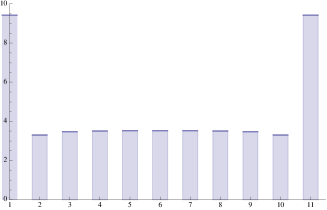
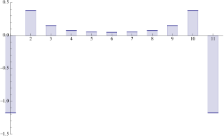
Figure 2: Optimal strategy $\bm{\xi}$ for $G$ as in Corollary 3.8 with $\kappa=1$, $\tilde{\kappa}=1.8$, $\rho=0.3$, $X_{0}=(-50,1)^{\top}$, $T=5$, and $N=11$. Left: $\xi^{1}_{1},\ldots,\xi^{1}_{11}$, right: $\xi^{2}_{1},\ldots,\xi^{2}_{11}$.

Corollary 3.8.

Let $\rho,\kappa,\widetilde{\kappa}>0$ and

$$G(t)=\begin{pmatrix}\exp(-\kappa t)&\rho\exp(-\widetilde{\kappa}t)\\ \rho\exp(-\widetilde{\kappa}t)&\exp(-\kappa t)\end{pmatrix}.$$

1. $G$ is nonnegative if and only if $\frac{\kappa}{\widetilde{\kappa}}\leq 1$ and $\rho\leq 1$.

2. $G$ is nonincreasing if and only if $\rho\leq\frac{\kappa}{\widetilde{\kappa}}\leq 1$. In this case, it is also nonnegative.

3. $G$ is convex if and only if $\rho\leq\frac{\kappa^{2}}{\widetilde{\kappa}^{2}}\leq 1$.

4. If $G$ is nonincreasing, $G$ is positive definite.

5. $G$ is commuting.

The following proposition shows that we cannot drop the assumption of symmetry in Theorem 2.15 in general.

Proposition 3.9.

Let

$$G(t)=\begin{pmatrix}\exp(-t\wedge 1)&\frac{1}{8}\exp(-2(t\wedge 1))\\ \frac{1}{8}\exp(-3(t\wedge 1))&\exp(-t\wedge 1)\end{pmatrix}.$$

$G$ is continuous, convex, nonincreasing, and nonnegative, but not positive definite.

3.3 Linear decay

In this section, we analyze linear decay of price impact for $K=2$ assets.

Proposition 3.10.

Let

$$G(t)=\begin{pmatrix}(a_{11}-b_{11}t)^{+}&(a_{12}-b_{12}t)^{+}\\ (a_{21}-b_{21}t)^{+}&(a_{22}-b_{22}t)^{+}\end{pmatrix}$$

with $a_{11},a_{12},a_{21},a_{22},b_{11},b_{12},b_{21},b_{22}>0$.

1. $G$ is nonnegative if and only if $\max\{\frac{a_{12}}{b_{12}},\frac{a_{21}}{b_{21}}\}\leq\min\{\frac{a_{11}}{b_{11}},\frac{a_{22}}{b_{22}}\}$ and $\frac{1}{4}(a_{12}+a_{21})^{2}\leq a_{11}a_{22}$.

2. $G$ is nonincreasing if and only if $\max\{\frac{a_{12}}{b_{12}},\frac{a_{21}}{b_{21}}\}\leq\min\{\frac{a_{11}}{b_{11}},\frac{a_{22}}{b_{22}}\}$ and $\frac{1}{4}(b_{12}+b_{21})^{2}\leq b_{11}b_{22}$.

3. Assume that $\max\{\frac{a_{12}}{b_{12}},\frac{a_{21}}{b_{21}}\}\leq\min\{\frac{a_{11}}{b_{11}},\frac{a_{22}}{b_{22}}\}$ and $a_{12}=a_{21}$. Then, $G$ is positive definite if and only if $G$ is symmetric (i.e. $a_{12}=a_{21}$ and $b_{12}=b_{21}$), $\frac{a_{11}}{b_{11}}=\frac{a_{12}}{b_{12}}=\frac{a_{22}}{b_{22}}$ and $b_{12}^{2}\leq b_{11}b_{22}$. In this case, we set $\lambda=\frac{a_{11}}{b_{11}}$ and have

   $$G(t)=(\lambda-t)^{+}\begin{pmatrix}b_{11}&b_{12}\\ b_{12}&b_{22}\end{pmatrix},$$

   and $G$ is also nonincreasing, convex, and commuting.

4 Conclusion

Our goal in this paper was to analyze a linear market impact model with transient price impact for $K$ different risky assets. We were in particular interested in the question which properties a decay kernel should satisfy so that the corresponding market impact model has certain desirable features and properties. Let us summarize some of the main messages for the practical application of transient price impact models that can be drawn from our results.

1. To exclude price manipulation in the sense of Huberman and Stanzl (2004) and to guarantee the existence of optimal strategies, decay kernels should be positive definite in the sense of Definition 2.9 (Propositions 2.6 and 2.7 and Lemma 2.8).

2. Requiring only positive definiteness is typically not sufficient to guarantee that optimal strategies are well-behaved (Figure 1). In particular, the nonparametric estimation of decay kernels can be problematic.

3. Assuming that the decay kernel is symmetric, nonnegative, nonincreasing, convex, and commuting guarantees that optimal strategies have many desirable properties and can easily be computed (Propositions 2.17 and 2.18). The additional assumption that $t\mapsto x^{\top}G(t)x$ is nonconstant for all $x\in\mathbb{R}^{K}$ guarantees that optimal strategies are unique (Theorem 2.15 and Proposition 2.7). In this setting, one can also optimize jointly over time grids and strategies and pass to a continuous-time limit.

4. Matrix functions (13) provide a convenient method for constructing decay kernels satisfying the properties from (c). Optimal strategies for matrix exponential decay can be computed in closed form (Example 3.5).

5. If the price impact between all asset pairs decay at a uniform rate, then cross-asset impact can be ignored and one can consider each asset individually (Propositions 3.1 and 3.2).

5 Proofs

Proof of Lemma 2.3.

Using the continuity of $G$ and the right-continuity of $S^{0}$, we have

$$-\mathbb{E}[\,\mathscr{R}(\bm{\xi})\,] = \mathbb{E}\Big{[}\,\frac{1}{2}\sum_{k=1}^{N}\xi_{k}^{\top}(S^{\bm{\xi}}_{t_{k}+}+S^{\bm{\xi}}_{t_{k}})\,\Big{]}$$

$$= \mathbb{E}\bigg{[}\,\sum_{k=1}^{N}\xi_{k}^{\top}S^{0}_{t_{k}}\,\bigg{]}+\mathbb{E}\bigg{[}\,\frac{1}{2}\sum_{k=1}^{N}\xi_{k}^{\top}G(0)\xi_{k}+\sum_{k=1}^{N}\sum_{\ell=1}^{k-1}\xi_{k}^{\top}G(t_{k}-t_{\ell})\xi_{\ell}\,\bigg{]}.$$

From the martingale property of $S^{0}$ and the requirement that $\sum_{k=1}^{N}\xi_{k}=-X_{0}$ we obtain that

$$\mathbb{E}\bigg{[}\,\sum_{k=1}^{N}\xi_{k}^{\top}S^{0}_{t_{k}}\,\bigg{]}=\mathbb{E}\Big{[}\,\sum_{k=1}^{N}\xi_{k}^{\top}S_{T}^{0}\,\Big{]}=-X_{0}^{\top}S^{0}_{0}.$$

Furthermore,

$$\frac{1}{2}\sum_{k=1}^{N}\xi_{k}^{\top}G(0)\xi_{k}+\sum_{k=1}^{N}\sum_{\ell=1}^{k-1}\xi_{k}^{\top}G(t_{k}-t_{\ell})\xi_{\ell}$$

$$= \frac{1}{2}\sum_{k=1}^{N}\xi_{k}^{\top}\widetilde{G}(0)\xi_{k}+\frac{1}{2}\sum_{k=1}^{N}\sum_{\ell=1}^{k-1}\xi_{k}^{\top}\widetilde{G}(t_{k}-t_{\ell})\xi_{\ell}+\frac{1}{2}\sum_{k=1}^{N}\sum_{\ell=1}^{k-1}\xi_{\ell}^{\top}\widetilde{G}(t_{\ell}-t_{k})\xi_{k}=C_{\mathbb{T}}(\bm{\xi}).$$

This proves (4). ∎

Proof of Lemma 2.4.

Suppose that a minimizer $\bm{\eta}\in\mathscr{X}(\mathbb{T},X_{0})$ of $\mathbb{E}[\,C_{\mathbb{T}}(\bm{\eta})\,]$ exists but that, by way of contradiction, there is no deterministic minimizer of $C_{\mathbb{T}}(\cdot)$. Then there can be no $\bm{\xi}\in\mathscr{X}_{\text{\rm det}}(\mathbb{T},X_{0})$ such that $C_{\mathbb{T}}(\bm{\xi})\leq\mathbb{E}[\,C_{\mathbb{T}}(\bm{\eta})\,]$. Since $\bm{\eta}(\omega)\in\mathscr{X}_{\text{\rm det}}(\mathbb{T},X_{0})$ for $\mathbb{P}$-a.e. $\omega$, we must thus have $C_{\mathbb{T}}(\bm{\eta}(\omega))>\mathbb{E}[\,C_{\mathbb{T}}(\bm{\eta})\,]$ for $\mathbb{P}$-a.e. $\omega\in\Omega$. But this is a contradiction. The proofs of the remaining assertions are also obvious and left to the reader. ∎

Proof of Proposition 2.6.

The equivalence of conditions (a) and (b) follows from Lemma 2.4.

To prove the equivalence of (b) and (c), it is sufficient to observe that $C_{\mathbb{T}}(\bm{\xi})$ is a quadratic form on $\mathbb{R}^{|\mathbb{T}|}\otimes\mathbb{R}^{K}$, and it is well known that a quadratic form is convex if and only if it is nonnegative.

We next prove the equivalence of (b) and (d). Clearly, (d) immediately implies (b) using the representation (5) of $C_{\mathbb{T}}(\cdot)$ and comparing it with (8) with $z_{i}\in\mathbb{R}^{K}$. For the proof of the converse implication, we fix $t_{1},\dots,t_{N}\in\mathbb{R}$. , Clearly we can assume without loss of generality that $\mathbb{T}=\{t_{1},\dots,t_{N}\}$ is a time grid in the sense that $0=t_{1}<t_{2}<\cdots<t_{N}$. An $N$-tuple $\bm{\zeta}:=(\zeta_{1},\dots,\zeta_{N})$ with $\zeta_{i}\in\mathbb{C}^{K}$ can be regarded as an element in the tensor product $\mathbb{C}^{N}\otimes\mathbb{C}^{K}$. Let us thus define the linear map ${\bm{L}}:\mathbb{C}^{N}\otimes\mathbb{C}^{K}\to\mathbb{C}^{N}\otimes\mathbb{C}^{K}$ by

$${\bm{L}}\bm{\zeta}=\Big{(}\sum_{j=1}^{N}\widetilde{G}(t_{1}-t_{j})\zeta_{j},\sum_{j=1}^{N}\widetilde{G}(t_{2}-t_{j})\zeta_{j},\dots,\sum_{j=1}^{N}\widetilde{G}(t_{N}-t_{j})\zeta_{j}\Big{)}.$$ (16)

We claim that ${\bm{L}}$ is Hermitian. Indeed, for $\bm{\eta},\bm{\zeta}\in\mathbb{C}^{N}\otimes\mathbb{C}^{K}$, the inner product in $\mathbb{C}^{N}\otimes\mathbb{C}^{K}$ between $\bm{\eta}$ and ${\bm{L}}\bm{\zeta}$ is given by

$$\langle\bm{\eta},{\bm{L}}\bm{\zeta}\rangle=\sum_{i,j=1}^{N}\eta_{i}^{*}\widetilde{G}(t_{i}-t_{j})\zeta_{j}=\sum_{i,j=1}^{N}\zeta_{j}^{*}\widetilde{G}(t_{i}-t_{j})^{*}\eta_{i}=\sum_{i,j=1}^{N}\zeta_{j}^{*}\widetilde{G}(t_{j}-t_{i})\eta_{i}=\langle\bm{\zeta},{\bm{L}}\bm{\eta}\rangle,$$

where we have used the fact that $\widetilde{G}(t_{i}-t_{j})^{*}=\widetilde{G}(t_{i}-t_{j})^{\top}=\widetilde{G}(t_{j}-t_{i})$. It follows that the restriction of ${\bm{L}}$ to $\mathbb{R}^{N}\otimes\mathbb{R}^{K}$ is symmetric and, due to condition (b), satisfies $0\leq C_{\mathbb{T}}(\bm{\xi})=\langle\bm{\xi},{\bm{L}}\bm{\xi}\rangle$ for all $\bm{\xi}\in\mathbb{R}^{N}\otimes\mathbb{R}^{K}$. By the symmetry of $\bm{L}$ and since $\bm{L}$ has only real entries, it follows that $\langle\bm{\zeta},{\bm{L}}\bm{\zeta}\rangle\geq 0$ for all $\bm{\zeta}\in\mathbb{C}^{N}\otimes\mathbb{C}^{K}$, which is the same as (8) and hence yields (d). The remaining assertions are obvious. ∎

Proof of Proposition 2.7.

We first show the existence of optimal strategies when $\widetilde{G}$ is positive definite. We will use the notation introduced in the proof of Proposition 2.6. For $X_{0}\in\mathbb{R}^{K}$ and $\mathbb{T}$ with $N=|\mathbb{T}|$ fixed, the minimization of $C_{\mathbb{T}}(\bm{\xi})$ over $\bm{\xi}\in\mathscr{X}_{\text{det}}(\mathbb{T},X_{0})$ is equivalent to the minimization of the symmetric and positive semidefinite quadratic form $\mathbb{R}^{N}\otimes\mathbb{R}^{K}\ni\bm{\xi}\mapsto\langle\bm{\xi},{\bm{L}}\bm{\xi}\rangle$ under the equality constraint $A\bm{\xi}=X_{0}$, where $\bm{L}$ is as in (16) and $A:\mathbb{R}^{N}\otimes\mathbb{R}^{K}\to\mathbb{R}^{K}$ is the linear map $A\bm{\xi}:=\sum_{k=1}^{N}\xi_{k}$. For fixed $\bm{\eta}\in\mathscr{X}_{\text{det}}(\mathbb{T},X_{0})$, every other $\bm{\xi}\in\mathscr{X}_{\text{det}}(\mathbb{T},X_{0})$ can be written as $\bm{\xi}=\bm{\eta}+\bm{\xi}^{0}$ for some $\bm{\xi}^{0}\in\mathscr{X}_{\text{det}}(\mathbb{T},0)$. Then, due to the symmetry of $\bm{L}$,

$$\langle\bm{\xi},{\bm{L}}\bm{\xi}\rangle=\langle\bm{\eta},{\bm{L}}\bm{\eta}\rangle+2\langle{\bm{L}}\bm{\eta},\bm{\xi}^{0}\rangle+\langle\bm{\xi}^{0},{\bm{L}}\bm{\xi}^{0}\rangle,$$

and our problem is now equivalent to the unconstraint minimization of the right-hand expression over $\bm{\xi}^{0}\in\mathscr{X}_{\text{det}}(\mathbb{T},0)$. Clearly, $\bm{L}\bm{\xi}^{0}=0$ implies that also $2\langle{\bm{L}}\bm{\eta},\bm{\xi}^{0}\rangle=2\langle\bm{\eta},{\bm{L}}\bm{\xi}^{0}\rangle=0$. Therefore the existence of minimizers follows from Section 2.4.2 in Boot (1964).

The uniqueness of optimal strategies for strictly positive definite $\widetilde{G}$ follows immediately from the strict convexity of $\bm{\xi}\mapsto C_{\mathbb{T}}(\bm{\xi})$ (see Proposition 2.6). The characterization of optimal strategies through Lagrange multipliers as in (9) is standard.∎

Proof of Lemma 2.8.

(a) That $H(0)$ is nonnegative definite follows by taking $N=1$ in (8). To show $H(-t)=H(t)^{*}$ for any given $t\in\mathbb{R}$ we take $N=2$ in (8) and let $t_{1}=0$ and $t_{2}=t$. It follows from the preceding assertion that $z_{1}^{*}H(-t)z_{2}+z_{2}^{*}H(t)z_{1}$ must be a real number for all $z_{1},z_{2}\in\mathbb{C}^{K}$. Taking $z_{1}=c_{1}e_{i}$ and $z_{2}=c_{2}e_{j}$ with $c_{k}\in\mathbb{C}$ and $e_{\ell}$ denoting the $\ell^{\text{th}}$ unit vector in $\mathbb{R}^{K}$ yields that $\overline{c_{1}}c_{2}H_{ij}(-t)+c_{1}\overline{c_{2}}H_{ji}(t)\in\mathbb{R}$, where $\overline{c}$ denotes the complex conjugate of $c\in\mathbb{C}$. Choosing $c_{1}=c_{2}=1$ gives $\operatorname{Im}(H_{ij}(-t))=-\operatorname{Im}(H_{ji}(t))$ and $c_{1}=1,c_{2}=i$ yields $\operatorname{Re}(H_{ij}(-t))=\operatorname{Re}(H_{ji}(t))$.

(b) For $t_{1},\dots,t_{N}\in\mathbb{R}$, we define $\tilde{t}_{i}=t_{N}-t_{N+1-i}$ and get from part (a) that for $\bm{\zeta}\in\mathbb{C}^{N}\otimes\mathbb{C}^{K}$

$$0 \leq \sum_{i,j=1}^{N}\zeta_{N+1-i}^{*}H(\tilde{t}_{i}-\tilde{t}_{j})\zeta_{N+1-j}=\sum_{i,j=1}^{N}\zeta_{N+1-i}^{*}H(-(t_{N+1-i}-t_{N+1-j}))\zeta_{N+1-j}$$

$$= \sum_{i,j=1}^{N}\zeta_{i}^{*}H(t_{i}-t_{j})^{*}\zeta_{j}.$$

∎

Proof of Corollary 2.11.

For the proof of implication (c)$\Rightarrow$(b), we note first that the matrix $M(d\gamma)$ is symmetric, as $M$ is nonnegative definite and $\mathbb{R}^{K\times K}$-valued. This implies that the matrix $H(t)$ is also symmetric for all $t$. Next, the symmetry of $M$ on $\mathbb{R}$ implies that the imaginary part of $\int_{\mathbb{R}}e^{i\gamma t}\,M_{k\ell}(d\gamma)$ is equal to $\int_{0}^{\infty}\big{(}\sin(t\gamma)+\sin(-t\gamma)\big{)}\,M_{k\ell}(d\gamma)=0$. Therefore, $H$ takes values in $\mathbb{R}^{K\times K}$ and, in turn, in $\mathbb{S}(K)$. We next define a finite $\mathbb{R}_{+}$-valued measure $\mu$ through $\mu(A):=x^{\top}M(A)x$ for $A\in\mathscr{B}(\mathbb{R})$. Then the function $t\mapsto x^{\top}H(t)x$ is the Fourier transform of $\mu$ and hence a positive definite function by Bochner’s theorem.

To prove (b)$\Rightarrow$(a), we will establish condition (b) of Theorem 2.10. To this end, write $z\in\mathbb{C}^{K}$ as $z=x+iw$, where $x,w\in\mathbb{R}^{K}$ and $i=\sqrt{-1}$. Then $z^{*}H(t)z=x^{\top}H(t)x+w^{\top}H(t)w$ due to the symmetry of $H(t)$. Hence $t\mapsto z^{*}H(t)z$ is the sum of two real-valued positive definite functions and therefore positive definite.

To prove (a)$\Rightarrow$(c), note that each component $H_{k\ell}$ of $H$ is equal to the Fourier transform of the complex measure $M_{k\ell}$. Since $M_{k\ell}$ is uniquely determined through $H_{k\ell}$ and since $H_{k\ell}=H_{\ell k}$ we must have that $M_{k\ell}=M_{\ell k}$. But a symmetric matrix can be nonnegative definite, and hence Hermitian, only if it is real. Therefore we must have $M(A)\in\mathbb{S}_{+}(K)$ for all $A\in\mathscr{B}(\mathbb{R})$. Finally, the fact that the symmetric positive definite matrix-valued function $H_{k\ell}$ takes only real values implies via Lemma 2.8 (a) that $H(-t)=H(t)$. Therefore, $H$ is equal to the Fourier transform of the measure $N(A):=\frac{1}{2}(M(A)+M(-A))$, $A\in\mathscr{B}(\mathbb{R})$. But, since $M$ is uniquely determined by $H$ according to Theorem 2.10, we get that $N=M$, and so $M$ must be symmetric on $\mathbb{R}$. ∎

Proof of Lemma 2.14.

We assume by way of contradiction that there exist $x\in\mathbb{R}^{K}$, $t^{*}>0$ and $\varepsilon>0$ such that $g^{x}(t):=x^{\top}G(t)x$ satisfies $g^{x}(t^{*})=-\varepsilon$. We are going to show that the function $g^{x}$ is not positive definite. Set $t_{k}=k\cdot t^{*}$ and $x_{k}=1$ for $k\in\mathbb{N}$. Since $|t_{k}-t_{l}|\geq t^{*}$ for $k\neq l$ and $g^{x}$ is nonincreasing, we have $g^{x}(|t_{k}-t_{l}|)\leq-\varepsilon$ for $k\neq l$. Thus, $\sum_{k,l=1}^{n}x_{k}x_{l}g^{x}(|t_{k}-t_{l}|)\leq ng^{x}(0)-(n^{2}-n)\,\varepsilon$. If $n$ is large enough, the latter expression is negative. Thus, $g^{x}$ is not positive definite, and so $G$ can not be positive definite. ∎

We now start preparing the proof of Theorem 2.15 and give a representation of a convex, nonincreasing, nonnegative, and symmetric function $G:[0,\infty)\to\mathbb{R}^{K\times K}$. To this end, let us first observe that, for such $G$, the limit $G(\infty):=\lim_{t\uparrow\infty}G(t)$ is well defined in the set of nonnegative definite matrices. Indeed, for any $x\in\mathbb{R}^{K}$, $g^{x}(t)=x^{\top}G(t)x$ is a convex, nonincreasing, nonnegative function and thus converges to a limit that we denote by $g^{x}(\infty)$. Let $e_{i}$ denote the $i^{\text{th}}$ unit vector. By polarization, we have $G_{ij}(t)=\frac{1}{4}(g^{e_{i}+e_{j}}(t)-g^{e_{i}-e_{j}}(t))$, and this expression converges to $G_{ij}(\infty)=\frac{1}{4}(g^{e_{i}+e_{j}}(\infty)-g^{e_{i}-e_{j}}(\infty))$. In particular, we have $g^{x}(\infty)=x^{\top}G(\infty)x$ for any $x\in\mathbb{R}^{K}$.

Proposition 5.1.

Let $G:[0,\infty)\to\mathbb{R}^{K\times K}$ be convex, nonincreasing, nonnegative, symmetric, and continuous. There exists a nonnegative Radon measure $\mu$ on $(0,\infty)$ and a measurable function $\Lambda:(0,\infty)\to\mathbb{S}_{+}(K)$ such that

$$G(t)=G(\infty)+\int_{(0,\infty)}(r-t)^{+}\Lambda(r)\,\mu(dr).$$ (17)

Furthermore, $G$ is the Fourier transform of the nonnegative definite matrix-valued measure

$$M(d\gamma)=G(\infty)\,\delta_{0}(d\gamma)+\Phi(\gamma)\,d\gamma,$$

where $\Phi:\mathbb{R}\to\mathbb{S}_{+}(K)$ is the continuous function given by

$$\Phi(x)=\frac{1}{\pi}\int_{(0,\infty)}\frac{1-\cos xy}{x^{2}}\Lambda(y)\,\mu(dy).$$

Proof.

By Lemmas 4.1 and 4.2 in Gatheral et al. (2012), we find that for every $x\in\mathbb{R}^{K}$ there is a Radon measure $\mu_{x}$ on $(0,\infty)$ such that

$$g^{x}(t)=g^{x}(\infty)+\int_{(0,\infty)}(r-t)^{+}\,\mu_{x}(dr),\qquad t>0.$$ (18)

Moreover, $g^{x}(t)$ is the Fourier transform of the following nonnegative Radon measure on $\mathbb{R}$

$$\mu_{x}(dt)=x^{\top}G(\infty)x\,\delta_{0}(dt)+\varphi_{x}(t)\,dt,$$ (19)

where $\delta_{0}$ is the Dirac measure concentrated in $0$ and

$$\varphi_{x}(t)=\frac{1}{\pi}\int_{(0,\infty)}\frac{1-\cos ty}{t^{2}}\,\mu_{x}(dy).$$ (20)

We consider the finite set $Z:=\{e_{i}\pm e_{j}\,|\,i,j=1,\dots,K\}$ and define $\mu=\sum_{z\in Z}\mu_{z}$. Then each $\mu_{z}$ with $z\in Z$ is absolutely continuous with respect to $\mu$ and has the Radon-Nikodym derivative $\lambda_{z}=d\mu_{z}/d\mu$. We set

$$\Lambda_{ij}(r):=\frac{1}{4}\Big{(}\lambda_{e_{i}+e_{j}}(r)-\lambda_{e_{i}-e_{j}}(r)\Big{)},\qquad r>0.$$ (21)

Clearly, $\Lambda_{ij}(r)=\Lambda_{ji}(r)$, and it remains to prove that $\Lambda$ is $\mu$-a.s. nonnegative definite. Let $x\in\mathbb{R}^{K}$. Since $g^{x}(t)=\frac{1}{4}\sum_{i,j=1}^{K}x_{i}x_{j}(g^{e_{i}+e_{j}}(t)-g^{e_{i}-e_{j}}(t))$, we necessarily have from (18):

$$g^{x}(t)-g^{x}(\infty)=\int_{(0,\infty)}(r-t)^{+}\,\mu_{x}(dr)=\int_{(0,\infty)}(r-t)^{+}\sum_{i,j=1}^{K}x_{i}x_{j}\Lambda_{ij}(r)\,\mu(dr),\qquad t>0.$$

Writing $(r-t)^{+}$ as $\int_{0}^{\infty}\mathbbmss{1}_{\{t\leq s<r\}}\,ds$, integrating by parts, and taking derivatives with respect to $t$ gives

$$0\leq\mu_{x}\big{(}(t,+\infty)\big{)}=\int_{(t,+\infty)}\sum_{i,j=1}^{K}x_{i}x_{j}\Lambda_{ij}(r)\,\mu(dr)$$

for any $t\geq 0$ and so $\sum_{i,j=1}^{K}x_{i}x_{j}\Lambda_{ij}(r)\geq 0$ for $r\not\in N_{x}$, where $N_{x}$ is such that $\mu(N_{x})=0$. We define $N=\bigcup_{x\in\mathbb{Q}^{K}}N_{x}$. Then $\mu(N)=0$ and, by continuity, $\sum_{i,j=1}^{K}x_{i}x_{j}\Lambda_{ij}(r)\geq 0$ for all $x\in\mathbb{R}^{K}$ and $r\not\in N$.

Now that we have shown $\mu_{x}(dr)=\sum_{i,j=1}^{K}x_{i}x_{j}\Lambda_{ij}(r)\,\mu(dr)$, we get (17) from (18). Next, we obtain from (20) that

$$\varphi_{x}(t)=\frac{1}{\pi}\int_{(0,\infty)}\frac{1-\cos ty}{t^{2}}\sum_{i,j=1}^{K}x_{i}x_{j}\Lambda_{ij}(y)\,\mu(dy).$$

Again, we define by polarization $\Phi(t)_{ij}=\frac{1}{4}(\varphi_{e_{i}+e_{j}}(t)-\varphi_{e_{i}-e_{j}}(t))$. We then have

$$\Phi(t)=\frac{1}{\pi}\int_{(0,\infty)}\frac{1-\cos ty}{t^{2}}\Lambda(y)\,\mu(dy),$$

and $\varphi_{x}(t)=x^{\top}\Phi(t)x$. Together with (19), this gives the claim. ∎

Proof of Theorem 2.15.

From Theorem 2.10 and the fact that $g^{x}$ is positive definite for each $x$, we already know that $G$ is positive definite. Note also that $G$ cannot be strictly positive definite if there exists some nonzero $x\in\mathbb{R}^{K}$ such that $t\mapsto x^{\top}G(t)x$ is constant, for then the choice $z_{1}=x$ and $z_{2}=-x$ gives $\sum_{i,j=1}^{2}z_{i}^{*}G(t_{i}-t_{j})z_{j}=0$ for all $t_{1},t_{2}\in\mathbb{R}$.

It thus remains to show that $G$ strictly definite positive if $\zeta^{\top}G(t)\zeta$ is nonconstant for any $\zeta\in\mathbb{R}^{K}$. We argue first that, in proving this assertion, we can assume without loss of generality that $G$ is continuous. To this end, consider again the functions $g^{x}(t):=x^{\top}G(t)x$ for $x\in\mathbb{R}^{K}$. As these functions are convex and nonincreasing, they are continuous on $(0,\infty)$ and admit right-hand limits, $g^{x}(0+):=\lim_{t\downarrow 0}g^{x}(t)\leq g^{x}(0)$. Using polarization as in the paragraph preceding Proposition 5.1, we thus conclude that $G$ is continuous on $(0,\infty)$, admits a right-hand limit $G(0+)$, and that $\Delta G(0):=G(0)-G(0+)$ is nonnegative definite. On the other hand, the continuous matrix-valued function $G^{cont}(t):=G(t+)$ also satisfies our assumptions and so will be strictly positive definite when the assertion has been established for continuous matrix-valued functions. But then $G(t)=G^{cont}(t)+\mathbbmss{1}_{\{0\}}(t)\Delta G(0)$ will also be strictly positive definite, because $\Delta G(0)$ is nonnegative definite.

Now, let $M$, $\Phi$, $\Lambda$, and $\mu$ be as in Proposition 5.1. It follows from this proposition that for $\bm{\zeta}=(\zeta_{1},\zeta_{2},\ldots,\zeta_{N})\in\mathbb{C}^{N}\otimes\mathbb{C}^{K}$ and $t_{1},t_{2},\ldots,t_{N}\in\mathbb{R}$

$$\sum_{k,\ell=1}^{N}\zeta_{k}^{*}\widetilde{G}(t_{k}-t_{\ell})\zeta_{\ell} =\sum_{k,\ell=1}^{N}\zeta_{k}^{*}\left(\int_{\mathbb{R}}e^{i(t_{k}-t_{\ell})\gamma}\,M(d{\gamma})\right)\zeta_{\ell}$$

$$=\Big{(}\sum_{k=1}^{N}\zeta_{k}\Big{)}^{*}G(\infty)\Big{(}\sum_{k=1}^{N}\zeta_{k}\Big{)}+\int\Big{(}\sum_{k=1}^{N}e^{-it_{k}\gamma}\zeta_{k}\Big{)}^{*}\Phi(\gamma)\Big{(}\sum_{k=1}^{N}e^{-it_{k}\gamma}\zeta_{k}\Big{)}\,d\gamma$$

$$=v(0)^{*}G(\infty)v(0)+\int v(\gamma)^{*}\Phi(\gamma)v(\gamma)\,d\gamma,$$

where $v(\gamma):=\sum_{k=1}^{N}e^{-it_{k}\gamma}\zeta_{k}$. We are now going to show that $\int v(\gamma)^{*}\Phi(\gamma)v(\gamma)\,d\gamma$ is strictly positive unless $\bm{\zeta}=0$. To this end, we note first that the components of the vector field $v(\cdot)$ are holomorphic functions of $\gamma\in\mathbb{C}$. When $\bm{\zeta}\neq 0$, at least one of these components is nonconstant and hence vanishes only for at most countably many $\gamma\in\mathbb{R}$. It follows that $v(\gamma)\neq 0$ for all but countably many $\gamma\in\mathbb{R}$. Moreover, we are going to argue next that the matrix $\Phi(\gamma)$ is strictly positive definite for all but countably many $\gamma\in\mathbb{R}$. Thus, $v(\gamma)^{*}\Phi(\gamma)v(\gamma)>0$ for Lebesgue-almost every $\gamma\in\mathbb{R}$, and it will follow that $\sum\zeta_{k}^{*}\widetilde{G}(t_{k}-t_{\ell})\zeta_{\ell}>0$.

So let us show now that the matrix $\Phi(\gamma)$ is strictly positive definite for all but countably many $\gamma\in\mathbb{R}$. To this end, we first note that for $z\in\mathbb{C}^{K}$

$$g^{z}(t)=z^{*}G(\infty)z+\int_{(0,\infty)}(r-t)^{+}z^{*}\Lambda(r)z\,\mu(dr).$$

Since the matrix $\Lambda(r)$ is nonnegative definite for all $r$, the fact that $g^{z}$ is nonconstant for $z\neq 0$ implies that

$$\int_{(0,\infty)}z^{*}\Lambda(r)z\,\mu(dr)>0\qquad\text{for $z\neq 0$.}$$ (22)

Now let $D$ be the set of all $y>0$ such that $\mu(\{y\})>0$, and let

$$\mu_{d}(E):=\mu(D\cap E)\quad\text{and}\quad\mu_{c}(E):=\mu(D^{c}\cap E)$$

be the discrete and continuous parts of $\mu$, respectively. Clearly,

$$N:=\big{\{}x\in\mathbb{R}\,\big{|}\,\cos xy=1\text{ for some $y\in D$}\big{\}}=\bigcup_{y\in D}\big{\{}x\in\mathbb{R}\,\big{|}\,\cos xy=1\big{\}}$$

is at most countable. Moreover, the set $\{y>0\,|\,\cos xy=1\}$ is a $\mu_{c}$-nullset for all $x\neq 0$. It thus follows that the measure $\frac{1-\cos xy}{x^{2}}\,\mu(dy)$ is equivalent to $\mu$ for all $x\notin N\cup\{0\}$. Therefore (22) implies that

$$z^{*}\Phi(x)z=\frac{1}{\pi}\int_{(0,\infty)}\frac{1-\cos xy}{x^{2}}z^{*}\Lambda(r)z\,\mu(dy)>0$$

for all $z\neq 0$ as long as $x\notin N\cup\{0\}$. This concludes the proof. ∎

Proof of Proposition 2.17.

We first prove (11). To this end, give a constructive proof for the existence of $O$. For $t\in\mathbb{R}$, we write $\mathbb{R}^{K}=E_{\lambda_{1}(t)}^{t}\oplus\dots\oplus E_{\lambda_{\ell(t)}(t)}^{t}$ for the orthogonal direct sum of the eigenspaces of $G(t)$ corresponding to the distinct eigenvalues $\lambda_{1}(t),\dots\lambda_{\ell(t)}(t)$ of $G(t)$. It follows from the commuting property that the eigenspaces of $G(t)$ are stable under the map $G(s)$, because $\lambda_{i}(t)G(s)v=G(t)G(s)v$ if $v\in E_{\lambda_{i}(t)}$.

Let $t_{1}\geq 0$ and define $D_{1}=\sum_{i=1}^{\ell(t_{1})}(\dim(E_{\lambda_{i}(t_{1})}^{t_{1}})-1)^{+}\leq K-1$. If for any $s\geq 0$ and $1\leq i\leq{\ell(t_{1})}$ there is $\mu_{i}(s)$ such that $G(s)v=\mu_{i}(s)v$ for any $v\in E_{\lambda_{i}(t_{1})}^{t_{1}}$, we are done by considering an orthonormal basis $(v^{1}_{i},\dots,v^{d_{i}}_{i})$ of each eigenspaces $E_{\lambda_{i}(t_{1})}^{t_{1}}$ and by setting $O=(v^{1}_{1},\dots,v^{d_{1}}_{1},\dots,v^{1}_{\ell},\dots,v^{d_{\ell}}_{\ell})$ for $\ell:=\ell(t_{1})$. This is necessarily the case if $D_{1}=0$. Otherwise, there is $t_{2}\geq 0$ such that, for at least one $i\in\{1,\dots,\ell(t_{1})\}$, the decomposition

$$E_{\lambda_{i}(t_{1})}^{t_{1}}=(E_{\lambda_{1}(t_{2})}^{t_{2}}\cap E_{\lambda_{i}(t_{1})}^{t_{1}})\oplus\dots\oplus(E_{\lambda_{\ell(t_{2})}(t_{2})}^{t_{2}}\cap E_{\lambda_{i}(t_{1})}^{t_{1}})$$

is such that

$$\dim(E_{\lambda_{i}(t_{1})}^{t_{1}})-1>\sum_{k=0}^{\lambda_{\ell(t_{2})}}\big{(}\dim(E_{\lambda_{k}(t_{2})}^{t_{2}}\cap E_{\lambda_{i}(t_{1})}^{t_{1}})-1\big{)}^{+}.$$

We write

$$\mathbb{R}^{K}=\bigoplus_{1\leq i_{1}\leq\ell(t_{1}),1\leq i_{2}\leq{\ell(t_{2})}}E_{\lambda_{i_{1}}(t_{1})}^{t_{1}}\cap E_{\lambda_{i_{2}}(t_{2})}^{t_{2}}$$

and have $D_{2}=\sum_{i_{1}=1}^{\ell(t_{1})}\sum_{i_{2}=1}^{\ell(t_{2})}(\dim(E_{\lambda_{i_{1}}(t_{1})}^{t_{1}}\cap E_{\lambda_{i_{2}}(t_{2})}^{t_{2}})-1)^{+}<D_{1}$. Once again, we are done if there is for any $s\geq 0$, $1\leq i_{1}\leq{\ell(t_{1})}$ and $1\leq i_{2}\leq{\ell(t_{2})}$, $\mu_{i_{1},i_{2}}(s)$ such that $G(s)v=\mu_{i_{1},i_{2}}(s)v$ for any $v\in E_{\lambda_{i_{1}}(t_{1})}^{t_{1}}\cap E_{\lambda_{i_{2}}(t_{2})}^{t_{2}}$. This is the case when $D_{2}=0$. Otherwise, there is $t_{3}$ such that

$$D_{3}=\sum_{i_{1}=1}^{\ell(t_{1})}\sum_{i_{2}=1}^{\ell(t_{2})}\sum_{i_{3}=1}^{\ell(t_{3})}\big{(}\dim(E_{\lambda_{i_{1}}(t_{1})}^{t_{1}}\cap E_{\lambda_{i_{2}}(t_{2})}^{t_{2}}\cap E_{\lambda_{i_{3}}(t_{3})}^{t_{3}})-1\big{)}^{+}<D_{2}$$

and we repeat this procedure at most $K$ times to get (11).

We now prove properties (a)—(e). Let $v_{i}$ be the $i^{\text{th}}$ column of $O$. Then $v_{i}$ is the eigenvector of $G_{i}(t)$ for the eigenvalue $g_{i}(t)$. A given $x\in\mathbb{R}^{K}$ can be written as $x=\sum_{i=1}^{K}\alpha_{i}v_{i}$. Then $Ox=\sum_{i=1}^{K}\alpha_{i}e_{i}$, where $e_{i}$ is the $i^{\text{th}}$ unit vector. It follows from (11) that $g^{x}(t)=\sum_{i=1}^{K}\alpha_{i}^{2}g_{i}(t)$. From here, the assertions (a)—(d) are obvious. Part (e) follows from Proposition 3.3. ∎

Proof of Proposition 2.18.

Let $O$ and $g_{1},\dots,g_{K}$ be as in Proposition 2.17. We let $v_{1},\dots,v_{K}$ be the columns of $O$. By Theorem 1 from Alfonsi et al. (2012) there is a one-dimensional optimal strategy $\bm{\eta}^{i}=(\eta^{i}_{1},\dots,\eta^{i}_{|\mathbb{T}|})\in\mathscr{X}_{\text{det}}(\mathbb{T},1)$ for the one-dimensional, nonincreasing, nonnegative, and convex decay kernel $g_{i}$, and $\bm{\eta}^{i}$ has only nonnegative components. By part (e) of Proposition 2.17, $\bm{\xi}^{(i)}:=\bm{\eta}^{i}v_{i}$ is an optimal strategy for $G$ in $\mathscr{X}_{\text{det}}(\mathbb{T},v_{i})$ that satisfies condition (a). When $X_{0}=\sum_{i=1}^{K}\alpha_{i}v_{i}\in\mathbb{R}^{K}$ is given, the strategy with components $\alpha_{i}{\bm{\eta}}^{i}v_{i}$ is an optimal strategy in $\mathscr{X}_{\text{\rm det}}(\mathbb{T},X_{0})$ by Proposition 2.17 (e).∎

Proof of Theorem 2.23.

The proof of part (a) can be performed along the lines of the proof of Theorem 2.20 from Gatheral et al. (2012) by noting that Proposition 2.18 (b) yields an upper bound on the number of shares traded by an optimal strategy $\bm{\xi}\in\mathscr{X}(\mathbb{S},X_{0})$ uniformly over finite time grids $\mathbb{S}\subset\mathbb{T}$:

$$\sum_{1\leq n\leq|\mathbb{S}|,1\leq j\leq K}|\xi^{j}_{n}|\leq\sum_{i=1}^{K}|\alpha_{i}|\sum_{j=1}^{K}|v^{j}_{i}|.$$

The details are left to the reader.

As for part (b), the argument from the proof of Theorem 2.20 in Gatheral et al. (2012) yields in particular, that $\mathbb{E}[\,C_{\mathbb{T}_{n}}(\bm{\xi}^{(n)})\,]$ decreases to $\mathbb{E}[\,C_{\mathbb{T}}(X^{*})\,]$ if $\mathbb{T}_{1}\subset\mathbb{T}_{2}\subset\cdots$ are finite time grids such that $\bigcup_{n}\mathbb{T}_{n}$ is dense in $\mathbb{T}$ and $\bm{\xi}^{(n)}$ is an optimal strategy in $\mathscr{X}(\mathbb{T}_{n},X_{0})$. This proves (b). ∎

Proof of Proposition 3.1.

Let $A\in\mathbb{R}^{K\times K}$ be a symmetric square root of the nonnegative definite matrix $L$ so that $L=A^{2}=A^{\top}A$. For $t_{1},\dots,t_{N}\in\mathbb{R}$ and $\zeta_{1},\dots,\zeta_{N}\in\mathbb{C}^{K}$ let $\eta_{k}:=A\zeta_{k}$. It follows that

$$\sum_{k,\ell=1}^{N}\zeta_{k}^{*}\widetilde{G}(t_{k}-t_{\ell})\zeta_{\ell}=\sum_{k,\ell=1}^{N}\zeta_{k}^{*}A^{\top}g(|t_{k}-t_{\ell}|)A\zeta_{\ell}=\sum_{k,\ell=1}^{N}\eta_{k}^{*}g(|t_{k}-t_{\ell}|)\eta_{\ell}=\sum_{i=1}^{K}\sum_{k,\ell=1}^{N}\overline{\eta}_{k}^{i}\eta_{\ell}^{i}g(|t_{k}-t_{\ell}|),$$

which is nonnegative since the function $g$ is positive definite. Now let $g$ and $L$ be even strictly positive definite. Then the matrix $A$ is nonsingular and so we have $\eta_{1}=\cdots=\eta_{N}=0$ if and only if $\zeta_{1}=\cdots=\zeta_{N}=0$. It follows that in all other cases the right-hand side above is strictly positive. ∎

Proof of Prop. 3.2.

Let $\bm{\xi}\in\mathscr{X}_{\text{det}}(\mathbb{T},X_{0})$ be an optimal strategy for the decay kernel $G$. By Proposition 2.7 there exists a Lagrange multiplier $\lambda\in\mathbb{R}^{K}$ such that

$$\sum_{\ell=1}^{N}\widetilde{G}(t_{k}-t_{\ell})\xi_{\ell}=\lambda\qquad\text{for $k=1,\dots,|\mathbb{T}|$.}$$

By multiplying both sides of this equation with $L$ we obtain

$$\sum_{\ell=1}^{N}\widetilde{G}_{L}(t_{k}-t_{\ell})\xi_{\ell}=L\lambda\qquad\text{for $k=1,\dots,|\mathbb{T}|$, }$$

which, again by Proposition 2.7, implies that $\bm{\xi}$ is also optimal for $G_{L}$. ∎

Proof of Proposition 3.3.

Since $L$ is invertible, the transformation

$$\bm{\xi}\longmapsto\bm{\xi}^{L}:=(L^{-1}\xi_{1},\dots,L^{-1}\xi_{|\mathbb{T}|})$$

is a one-to-one map from $\mathscr{X}_{\text{\rm det}}(\mathbb{T},LX_{0})$ to $\mathscr{X}_{\text{\rm det}}(\mathbb{T},X_{0})$. We also have

$$0\leq\sum_{k,\ell}\xi_{k}^{\top}\widetilde{G}(t_{k}-t_{\ell})\xi_{\ell}=\sum_{k,\ell}(\xi^{L}_{k})^{\top}\widetilde{G}^{L}(t_{k}-t_{\ell})\xi_{\ell}^{L}$$

for all $\mathbb{T}$ and $\bm{\xi}$. Minimizing the two sums over the respective classes of strategies yields the result. ∎

To study the examples for $K=2$ assets, we will frequently use the following simple lemma.

Lemma 5.2.

For $a,d\geq 0$ and $b,c\in\mathbb{R}$, the matrix $M:=\leavevmode\hbox{$\left(\begin{smallmatrix}a&b\\ c&d\end{smallmatrix}\right)$}$ is nonnegative if and only if $\frac{1}{4}(b+c)^{2}\leq ad$. When $b\in\mathbb{C}$, the Hermitian matrix $N:=\left(\begin{smallmatrix}a&b\\ \bar{b}&d\end{smallmatrix}\right)$ is nonnegative definite if and only if $|b|^{2}\leq ad$.

Proof.

The matrix $M$ is nonnegative if and only if its symmetrization, $\widetilde{M}:=\frac{1}{2}(M+M^{\top})$, is positive definite. Since a symmetric matrix is nonnegative definite if and only if all its leading principle minors are nonnegative and since $\det\widetilde{M}=ad-\frac{1}{4}(b+c)^{2}$, the result follows. In the Hermitian case, the same condition on the minors holds. ∎

Lemma 5.3.

Let $G:[0,\infty)\rightarrow\mathbb{R}^{K\times K}$ and assume that $G(t)=\int_{0}^{t}\Lambda(s)ds$ for $t\geq 0$. Then, $G$ is nonincreasing if and only if $-\Lambda(s)$ is nonnegative for a.e. $s$. If in addition $\Lambda$ is piecewise continuous, then $G$ is convex if and only if $-\Lambda$ is nonincreasing.

Proof.

The function $G$ is nonincreasing if and only if for any $\zeta\in\mathbb{R}^{K}$, $\int_{0}^{t}\zeta^{\top}\Lambda(s)\zeta ds$ is nonincreasing. This gives $\zeta^{\top}\Lambda(s)\zeta\geq 0$ for $s\not\in N_{\zeta}$, where $N_{\zeta}$ is a set with zero Lebesgue measure. We define $N=\cup_{\zeta\in\mathbb{Q}^{K}}N_{\zeta}$ and have by continuity $\zeta^{\top}\Lambda(s)\zeta\geq 0$ for any $s\not\in N$, $\zeta\in\mathbb{R}^{K}$. The converse implication as well as the other equivalence are obvious. ∎

Proof of Proposition 3.7.

(a): By Lemma 5.2, $G$ is nonnegative if and only if for every $t\geq 0$

$$\frac{1}{4}(a_{12}\exp(-b_{12}t)+a_{21}\exp(-b_{21}t))^{2}\leq a_{11}\exp(-b_{11}t)a_{22}\exp(-b_{22}t).$$

That is, if and only if

$$\frac{1}{4}(a_{12}^{2}\exp(-2b_{12}t)+2a_{12}a_{21}\exp(-(b_{12}+b_{21})t)+a_{21}^{2}\exp(-2b_{21}t))\leq a_{11}a_{22}\exp(-(b_{11}+b_{22})t).$$

If $G$ is nonnegative, taking $t=0$ shows $\frac{1}{4}(a_{12}+a_{21})^{2}\leq a_{11}a_{22}$, while sending $t\rightarrow\infty$ shows $\min\{b_{12},b_{21}\}\geq\frac{1}{2}(b_{11}+b_{22})$. Conversely, if these inequalities hold, $G$ is nonnegative.

(b): $G$ is continuously differentiable. By Lemma 5.3, $G$ is hence nonincreasing if and only if for every $t\geq 0$

$$-G^{\prime}(t)=\begin{pmatrix}a_{11}b_{11}\exp(-b_{11}t)&a_{12}b_{12}\exp(-b_{12}t)\\ a_{21}b_{21}\exp(-b_{21}t)&a_{22}b_{22}\exp(-b_{22}t)\end{pmatrix}$$

is nonnegative. Analogously to (a), the result follows.

(c): Analogously to (b), by Lemma 5.3 $G$ is convex if and only if for every $\geq 0$ its second derivative

$$G^{\prime\prime}(t)=\begin{pmatrix}a_{11}b_{11}^{2}\exp(-b_{11}t)&a_{12}b_{12}^{2}\exp(-b_{12}t)\\ a_{21}b_{21}^{2}\exp(-b_{21}t)&a_{22}b_{22}^{2}\exp(-b_{22}t)\end{pmatrix}$$

is nonnegative. The result follows analogously to (a).

(d): The assumption $a_{12}=a_{21}$ gives the continuity of $\widetilde{G}$. We have that $\widetilde{G}(t)=\int_{\mathbb{R}}e^{i\gamma t}M(d\gamma)$, where $M(d\gamma)=\frac{1}{2\pi}\Lambda(\gamma)\,d\gamma$ with the Hermitian matrix

$$\Lambda(\gamma)=\begin{pmatrix}2\frac{a_{11}b_{11}}{b_{11}^{2}+\gamma^{2}}&\frac{a_{12}}{b_{21}-i\gamma}+\frac{a_{12}}{b_{12}+i\gamma}\\ \frac{a_{12}}{b_{12}-i\gamma}+\frac{a_{12}}{b_{21}+i\gamma}&2\frac{a_{22}b_{22}}{b_{22}^{2}+\gamma^{2}}\end{pmatrix}.$$

From Theorem 2.10, $G$ is positive definite if and only if the matrix $\Lambda(\gamma)$ is nonnegative for almost all $\gamma\in\mathbb{R}$. According to Lemma 5.2, this is equivalent to

$$\frac{a_{12}^{2}(b_{12}+b_{21})^{2}}{(b_{12}^{2}+\gamma^{2})(b_{21}^{2}+\gamma^{2})}\leq 4\frac{a_{11}b_{11}}{b_{11}^{2}+\gamma^{2}}\frac{a_{22}b_{22}}{b_{22}^{2}+\gamma^{2}}.$$

This condition is in turn equivalent to

$${a_{12}^{2}(b_{12}+b_{21})^{2}}(b_{11}^{2}+\gamma^{2})(b_{22}^{2}+\gamma^{2})\leq 4{a_{11}b_{11}}{a_{22}b_{22}}{(b_{12}^{2}+\gamma^{2})(b_{21}^{2}+\gamma^{2})}.$$

Comparing the coefficients for $\gamma^{0}$, $\gamma^{2}$ and $\gamma^{4}$, we see that it is sufficient to have

$$a_{12}^{2}(b_{12}+b_{21})^{2}b_{11}b_{22} \leq 4a_{11}a_{22}b_{12}^{2}b_{21}^{2}$$ (23)

$$a_{12}^{2}(b_{12}+b_{21})^{2}(b_{11}^{2}+b_{22}^{2}) \leq 4a_{11}b_{11}a_{22}b_{22}(b_{12}^{2}+b_{21}^{2})$$ (24)

$$a_{12}^{2}(b_{12}+b_{21})^{2} \leq 4a_{11}b_{11}a_{22}b_{22}.$$ (25)

Note that (25) follows immediately from (b), since $G$ is nonincreasing and $a_{12}=a_{21}$. To show (23), note that $\sqrt{b_{11}b_{22}}\leq\frac{1}{2}(b_{11}+b_{22})\leq\min\{b_{12},b_{21}\}$, so $b_{11}b_{22}\leq(\min\{b_{12},b_{21}\})^{2}\leq b_{12}b_{21}$. Together with (25) the result follows. Now, we claim that $b_{11}^{2}+b_{22}^{2}\leq b_{12}^{2}+b_{21}^{2}$, which together with (25) gives (24). To see this, we define $m=\min\{b_{12},b_{21}\}$ and assume without loss of generality that $b_{11}\leq b_{22}$. Since $\frac{1}{2}(b_{11}+b_{22})\leq m$, we have $b_{11}\in(0,m]$ and $b_{11}^{2}+b_{22}^{2}\leq(2m-b_{11})^{2}+b_{11}^{2}\leq 2m^{2}$ because the polynomial function $x\in[0,m]\mapsto(2m-x)^{2}+x^{2}$ reaches its maximum for $x\in\{0,m\}$.

(e): We find that the left upper entry of $G(0)G(t)-G(t)G(0)$ is $a_{12}a_{21}(e^{-b_{21}t}-e^{-b_{12}t})$, so $G(0)G(t)=G(t)G(0)$ implies $b_{12}=b_{21}$. Given that, a direct calculation shows that $G(0)G(t)=G(t)G(0)$ is equivalent to $a_{11}(e^{-b_{11}t}-e^{-b_{12}t})+a_{22}(e^{-b_{12}t}-e^{-b_{22}t})=0$. If $a_{11}=a_{22}$, this implies $b_{11}=b_{22}$. If $a_{11}\neq a_{22}$, by the equivalent equation $a_{22}-a_{11}=a_{22}e^{-(b_{22}-b_{12})t}-a_{11}e^{-(b_{11}-b_{12})t}$ we see that $b_{11}=b_{22}=b_{12}$.

Conversely, if either $a_{11}=a_{22}$ and $b_{12}=b_{21}$ and $b_{11}=b_{22}$, or $b_{11}=b_{12}=b_{21}=b_{22}$, a direct calculation shows that $G(s)G(t)=G(t)G(s)$ for all $s,t\geq 0$. ∎

Proof of Proposition 3.9.

$G$ is obviously continuous and Proposition 3.7 yields that $G$ is nonnegative, nonincreasing and convex since $-G^{\prime}$ is nonincreasing.

To show that $G$ is not positive definite, using Mathematica we find that $G(t)=\int_{\mathbb{R}}e^{i\gamma t}M(d\gamma)$, where $M(d\gamma)=C\Lambda(\gamma)\,d\gamma+D\delta_{0}(d\gamma)$ with a constant $C>0$, a matrix $D\in\mathbb{R}^{2\times 2}$, the Dirac measure $\delta_{0}$ at $0$ and $\Lambda(\gamma)$ given by

$$\begin{pmatrix}\frac{2e^{2}(-\cos(\gamma)\gamma+e\gamma-\sin(\gamma))}{\gamma^{3}+\gamma}&\frac{5e^{3}\gamma-((3+2e)\gamma+6i(-1+e))\cos(\gamma)+(i(-3+2e)\gamma-6(1+e))\sin(\gamma)}{8\gamma(\gamma(\gamma+i)+6)}\\ \frac{5e^{3}\gamma-(3(\gamma+2i)+2e(\gamma-3i))\cos(\gamma)+(-2ie\gamma+3i\gamma-6e-6)\sin(\gamma)}{8\gamma(\gamma+2i)(\gamma-3i)}&\frac{2e^{2}(-\cos(\gamma)\gamma+e\gamma-\sin(\gamma))}{\gamma^{3}+\gamma}\\ \end{pmatrix}.$$

If $G$ was positive definite, then all eigenvalues of $\Lambda(\gamma)$ would be positive for $\gamma\neq 0$. But using Mathematica we find that one eigenvalue of $\Lambda(\gamma)$ is

$$\frac{1}{8\left(\gamma^{2}+4\right)\left(\gamma^{2}+9\right)\left(\gamma^{3}+\gamma\right)^{2}}\Big{(}16e^{3}\left(\gamma^{2}+1\right)\left(\gamma^{2}+4\right)\left(\gamma^{2}+9\right)\gamma^{2}$$

$$-16e^{2}\left(\gamma^{2}+1\right)\left(\gamma^{2}+4\right)\left(\gamma^{2}+9\right)\gamma(\sin(\gamma)+\gamma\cos(\gamma))$$

$$-\Big{(}\gamma^{2}\left(\gamma^{2}+1\right)^{4}\left(\gamma^{2}+4\right)\left(\gamma^{2}+9\right)\Big{(}\left(9+4e^{2}+25e^{6}\right)\gamma^{2}$$

$$-10e^{3}(3+2e)\gamma^{2}\cos(\gamma)+12e\left(\gamma^{2}-6\right)\cos(2\gamma)$$

$$-60e\gamma\sin(\gamma)\left(-2\cos(\gamma)+e^{3}+e^{2}\right)+36\left(1+e^{2}\right)\Big{)}\Big{)}^{\frac{1}{2}}\Big{)},$$

which is negative for all $\gamma$ with $0<|\gamma|<0.02$. So $G$ is not positive definite. ∎

Proof of Proposition 3.10.

(a): By Lemma 5.2, $G$ is nonnegative if and only if for every $t\geq 0$

$$\frac{1}{4}((a_{12}-b_{12}t)^{+}+(a_{21}-b_{21}t)^{+})^{2}\leq(a_{11}-b_{11}t)^{+}(a_{22}-b_{22}t)^{+}.$$

Assume that $G$ is nonnegative. Choosing $t=0$ yields $\frac{1}{4}(a_{12}+a_{21})^{2}\leq a_{11}a_{22}$. Choosing $t=\min\{\frac{a_{11}}{b_{11}},\frac{a_{22}}{b_{22}}\}$ yields that the right-hand side of the preceding equation is zero. So the left-hand side has to be zero which implies that $\max\{\frac{a_{12}}{b_{12}},\frac{a_{21}}{b_{21}}\}\leq t$.

Conversely, assume that $\frac{1}{4}(a_{12}+a_{21})^{2}\leq a_{11}a_{22}$ and $\max\{\frac{a_{12}}{b_{12}},\frac{a_{21}}{b_{21}}\}\leq\min\{\frac{a_{11}}{b_{11}},\frac{a_{22}}{b_{22}}\}$. So for any $t\geq 0$, we have that $\max\{(1-\frac{b_{12}}{a_{12}}t)^{+},(1-\frac{b_{21}}{a_{21}}t)^{+}\}\leq\min\{(1-\frac{b_{11}}{a_{11}}t)^{+},(1-\frac{b_{22}}{a_{22}}t)^{+}\}$. Thus,

$$\frac{1}{4}((a_{12}-b_{12}t)^{+}+(a_{21}-b_{21}t)^{+})^{2} = \frac{1}{4}\left(a_{12}\left(1-\frac{b_{12}}{a_{12}}t\right)^{+}+a_{21}\left(1-\frac{b_{21}}{a_{21}}t\right)^{+}\right)^{2}$$

$$\leq \frac{1}{4}\left((a_{12}+a_{21})\max\left\{\left(1-\frac{b_{12}}{a_{12}}t\right)^{+},\left(1-\frac{b_{21}}{a_{21}}t\right)^{+}\right\}\right)^{2}$$

$$\leq a_{11}a_{22}\left(\min\left\{\left(1-\frac{b_{11}}{a_{11}}t\right)^{+},\left(1-\frac{b_{22}}{a_{22}}t\right)^{+}\right\}\right)^{2}$$

$$\leq a_{11}a_{22}\left(1-\frac{b_{11}}{a_{11}}t\right)^{+}\left(1-\frac{b_{22}}{a_{22}}t\right)^{+}$$

$$= (a_{11}-b_{11}t)^{+}(a_{22}-b_{22}t)^{+}.$$

So $G$ is nonnegative.

(b): $G$ is absolutely continuous with derivative

$$G^{\prime}(t)=\begin{pmatrix}-b_{11}\mathbbmss{1}_{\{t<\frac{a_{11}}{b_{11}}\}}&-b_{12}\mathbbmss{1}_{\{t<\frac{a_{12}}{b_{12}}\}}\\ -b_{21}\mathbbmss{1}_{\{t<\frac{a_{21}}{b_{21}}\}}&-b_{22}\mathbbmss{1}_{\{t<\frac{a_{22}}{b_{22}}\}}\end{pmatrix}$$

By Lemmas 5.2 and 5.3, $G$ is nonincreasing if and only if for almost all $t>0$

$$\frac{1}{4}(b_{12}\mathbbmss{1}_{\{t<\frac{a_{12}}{b_{12}}\}}+b_{21}\mathbbmss{1}_{\{t<\frac{a_{21}}{b_{21}}\}})^{2}\leq b_{11}\mathbbmss{1}_{\{t<\frac{a_{11}}{b_{11}}\}}b_{22}\mathbbmss{1}_{\{t<\frac{a_{22}}{b_{22}}\}}.$$

Assume $G$ is nonincreasing. Then choosing $t$ small enough shows $\frac{1}{4}(b_{12}+b_{21})^{2}\leq b_{11}b_{22}$. Choosing any $t\geq\min\{\frac{a_{11}}{b_{11}},\frac{a_{22}}{b_{22}}\}$ yields that the right-hand side of the preceding equation is zero. So the left-hand-side has to be zero which implies $\max\{\frac{a_{12}}{b_{12}},\frac{a_{21}}{b_{21}}\}\leq\min\{\frac{a_{11}}{b_{11}},\frac{a_{22}}{b_{22}}\}$.

Conversely, if $\frac{1}{4}(b_{12}+b_{21})^{2}\leq b_{11}b_{22}$ and $\max\{\frac{a_{12}}{b_{12}},\frac{a_{21}}{b_{21}}\}\leq\min\{\frac{a_{11}}{b_{11}},\frac{a_{22}}{b_{22}}\}$, it is obvious that $G$ is nonincreasing.

(c): By computing the inverse Fourier transform, we easily get that for $a,b_{+},b->0$,

$$\mathbbmss{1}_{\{t\geq 0\}}(a-b_{+}t)^{+}+\mathbbmss{1}_{\{t<0\}}(a+b_{-}t)^{+}=\int_{\mathbb{R}}e^{i\gamma t}\frac{1}{2\pi\gamma^{2}}\left(b_{+}(1-e^{-\frac{a\gamma}{b_{+}}})+b_{-}(1-e^{\frac{a\gamma}{b_{-}}})\right)d\gamma.$$

Thanks to the assumption $a_{12}=a_{21}$, $\widetilde{G}$ is continuous and $\widetilde{G}(t)=\int_{\mathbb{R}}e^{i\gamma t}M(d\gamma)$ with $M(d\gamma)=\frac{1}{2\pi\gamma^{2}}\Lambda(\gamma)d\gamma$, with the Hermitian matrix

$$\Lambda(\gamma)=\begin{pmatrix}2b_{11}(1-\cos(\frac{a_{11}}{b_{11}}\gamma))&b_{12}(1-e^{\frac{-ia_{12}\gamma}{b_{12}}})+b_{21}(1-e^{\frac{ia_{12}\gamma}{b_{21}}})\\ b_{21}(1-e^{\frac{-ia_{12}\gamma}{b_{21}}})+b_{12}(1-e^{\frac{ia_{12}\gamma}{b_{12}}})&2b_{22}(1-\cos(\frac{a_{22}}{b_{22}}\gamma))\end{pmatrix}.$$

From Theorem 2.10, $G$ is positive definite if and only if $\Lambda(\gamma)$ is positive definite for every $\gamma\in\mathbb{R}$. Using Lemma 5.2, $\Lambda(\gamma)$ is positive definite if and only if

$$|b_{12}(1-e^{\frac{-ia_{12}\gamma}{b_{12}}})+b_{21}(1-e^{\frac{ia_{12}\gamma}{b_{21}}})|^{2}\leq b_{11}(1-\cos(\frac{a_{11}}{b_{11}}\gamma))b_{22}(1-\cos(\frac{a_{22}}{b_{22}}\gamma)),$$

i.e. if and only if

$$\left(b_{12}(1-\cos(\frac{a_{12}}{b_{12}}\gamma))+b_{21}(1-\cos(\frac{a_{12}}{b_{21}}\gamma))\right)^{2}+\left(b_{12}\sin(\frac{a_{12}}{b_{12}}\gamma)-b_{21}\sin(\frac{a_{12}}{b_{21}}\gamma)\right)^{2}$$

$$\leq 4b_{11}(1-\cos(\frac{a_{11}}{b_{11}}\gamma))b_{22}(1-\cos(\frac{a_{22}}{b_{22}}\gamma)),$$

which is equivalent to

$$\frac{a_{11}}{b_{11}}=\frac{a_{12}}{b_{12}}=\frac{a_{21}}{b_{21}}=\frac{a_{22}}{b_{22}},\ b_{12}^{2}\leq b_{11}b_{22}.$$

One implication is obvious. To see the other one, we apply the condition to $\gamma=2\pi\frac{b_{11}}{a_{11}}$, which gives $\frac{a_{12}b_{11}}{b_{12}a_{11}}\in\mathbb{N}$ and $\frac{a_{21}b_{11}}{b_{21}a_{11}}\in\mathbb{N}$, and thus $\frac{a_{12}b_{11}}{b_{12}a_{11}}=\frac{a_{21}b_{11}}{b_{21}a_{11}}=1$ since $\max\{\frac{a_{12}}{b_{12}},\frac{a_{21}}{b_{21}}\}\leq\min\{\frac{a_{11}}{b_{11}},\frac{a_{22}}{b_{22}}\}$ by assumption. Similarly, considering $\gamma=2\pi\frac{b_{22}}{a_{22}}$ gives $\frac{a_{12}b_{22}}{b_{12}a_{22}}=\frac{a_{21}b_{22}}{b_{21}a_{22}}=1$. In particular, $b_{12}=b_{21}$ and the condition for $\gamma=0$ gives the inequality on $b$’s. The remainder is obvious. ∎

References

- Alfonsi and Schied (2010) A. Alfonsi and A. Schied. Optimal trade execution and absence of price manipulations in limit order book models. SIAM J. Financial Math., 1:490–522, 2010.
- Alfonsi et al. (2008) A. Alfonsi, A. Fruth, and A. Schied. Constrained portfolio liquidation in a limit order book model. Banach Center Publications, 83:9–25, 2008.
- Alfonsi et al. (2010) A. Alfonsi, A. Fruth, and A. Schied. Optimal execution strategies in limit order books with general shape functions. Quant. Finance, 10:143–157, 2010.
- Alfonsi et al. (2012) A. Alfonsi, A. Schied, and A. Slynko. Order book resilience, price manipulation, and the positive portfolio problem. SIAM J. Finan. Math., 3(1):511–533, 2012.
- Almgren and Chriss (2001) R. Almgren and N. Chriss. Optimal execution of portfolio transactions. Journal of Risk, 3(2):5–39, 2001.
- Bertsimas and Lo (1998) D. Bertsimas and A. Lo. Optimal control of execution costs. Journal of Financial Markets, 1:1–50, 1998.
- Bochner (1932) S. Bochner. Vorlesungen über Fouriersche Integrale. Akademische Verlagsgesellschaft, Leipzig, 1932.
- Boot (1964) J. C. G. Boot. Quadratic programming. Algorithms, anomalies, applications. Studies in Mathematical and Managerial Economics, Vol. 2. North-Holland Publishing Co., Amsterdam, 1964.
- Bouchaud et al. (2004) J.-P. Bouchaud, Y. Gefen, M. Potters, and M. Wyart. Fluctuations and response in financial markets: the subtle nature of ’random’ price changes. Quantitative Finance, 4:176–190, 2004.
- Busseti and Lillo (2012) E. Busseti and F. Lillo. Calibration of optimal execution of financial transactions in the presence of transient market impact. Journal of Statistical Mechanics: Theory and Experiment, 2012(09):P09010, 2012.
- CFTC-SEC (2010) CFTC-SEC. Findings regarding the market events of May 6, 2010. Report, 2010.
- Cramér (1940) H. Cramér. On the theory of stationary random processes. Annals of Mathematics, 41(1):215–230, 1940.
- Donoghue (1974) W. F. Donoghue, Jr. Monotone matrix functions and analytic continuation. Springer-Verlag, New York, 1974. Die Grundlehren der mathematischen Wissenschaften, Band 207.
- Falb (1969) P. Falb. On a theorem of Bochner. Publications Mathématiques de l’IHÉS, 36(1):59–67, 1969.
- Fruth et al. (2014) A. Fruth, T. Schöneborn, and M. Urusov. Optimal trade execution and price manipulation in order books with time-varying liquidity. Mathematical Finance, 24:651–695, 2014.
- Gatheral (2010) J. Gatheral. No-Dynamic-Arbitrage and Market Impact. Quantitative Finance, 10:749–759, 2010.
- Gatheral and Schied (2013) J. Gatheral and A. Schied. Dynamical models of market impact and algorithms for order execution. In J.-P. Fouque and J. Langsam, editors, Handbook on Systemic Risk, pages 579–602. Cambridge University Press, 2013.
- Gatheral et al. (2012) J. Gatheral, A. Schied, and A. Slynko. Transient linear price impact and Fredholm integral equations. Mathematical Finance, 22(3):445–474, July 2012.
- Gihman and Skorohod (1974) I. Gihman and A. Skorohod. The Theory of Stochastic Processes I. Springer-Verlag, 1974.
- Gill et al. (1981) P. E. Gill, W. Murray, and M. H. Wright. Practical optimization. Academic Press Inc. [Harcourt Brace Jovanovich Publishers], London, 1981.
- Glöckner (2003) H. Glöckner. Positive definite functions on infinite-dimensional convex cones. Mem. Amer. Math. Soc., 166(789):xiv+128, 2003.
- Guo (2013) X. Guo. Optimal placement in a limit order book. In H. Topaloglu, editor, TUTORIALS in Operations Research, volume 10, pages 191–200. 2013.
- Huberman and Stanzl (2004) G. Huberman and W. Stanzl. Price Manipulation and Quasi-Arbitrage. Econometrica, 74(4):1247–1275, July 2004.
- Kratz and Schöneborn (2013) P. Kratz and T. Schöneborn. Optimal liquidation in dark pools. EFA 2009 Bergen Meetings Paper. SSRN, 2013. URL http://ssrn.com/abstract=1344583.
- Løkka (2012) A. Løkka. Optimal execution in a multiplicative limit order book. preprint, 2012.
- Moro et al. (2009) E. Moro, J. Vicente, L. G. Moyano, A. Gerig, J. D. Farmer, G. Vaglica, F. Lillo, and R. N. Mantegna. Market impact and trading profile of hidden orders in stock markets. Physical Review E, 80(6):066–102, 2009.
- Naimark (1943) M. Naimark. Positive definite operator functions on a commutative group. Bull. Acad. Sci. URSS Sér. Math. [Izvestia Akad. Nauk SSSR], 7:237–244, 1943.
- Obizhaeva and Wang (2013) A. Obizhaeva and J. Wang. Optimal trading strategy and supply/demand dynamics. Journal of Financial Markets, 16:1–32, 2013.
- Pólya (1949) G. Pólya. Remarks on characteristic functions. In J. Neyman, editor, Proceedings of the Berkeley Symposium of Mathematical Statistics and Probability, pages 115–123. University of California Press, 1949.
- Predoiu et al. (2011) S. Predoiu, G. Shaikhet, and S. Shreve. Optimal execution in a general one-sided limit-order book. SIAM J. Financial Math., 2:183–212, 2011.
- Sasvári (2013) Z. Sasvári. Multivariate characteristic and correlation functions, volume 50 of de Gruyter Studies in Mathematics. Walter de Gruyter & Co., Berlin, 2013.
- Schied et al. (2010) A. Schied, T. Schöneborn, and M. Tehranchi. Optimal basket liquidation for CARA investors is deterministic. Applied Mathematical Finance, 17:471–489, 2010.
- Schöneborn (2011) T. Schöneborn. Adaptive basket liquidation. Preprint, 2011.
- Young (1913) W. H. Young. On the Fourier series of bounded functions. Proceedings of the London Mathematical Society (2), 12:41–70, 1913.